2.1 Site description

Our study site is a created storm water wetland Gateway, located by an eutrophicated lake Enäjärvi in the district of Nummela, municipality of Vihti, Southern Finland (60.3272^∘ N, 24.3369^∘ E). Southern Finland experiences a climate with a 30-year mean air temperature of 4.6 ^∘C and an annual precipitation rate of 627 mm in the period of year 1981–2010 (Pirinen et al., 2012).

The wetland was constructed in 2010 at the mouth of a 550 ha largely urbanized (35 % impervious) watershed of Kilsoi stream. It was excavated over 6 weeks in early winter 2010 on an abandoned agricultural field growing meadow vegetation. All of the old drainage ditches were blocked as amphibian habitats, which also ensured only one inlet route receiving water from Kilsoi stream and one outlet route discharging water to the nearby lake Enäjärvi. Lake Enäjärvi is an eutrophicated lake. The internal phosphorus load from human activities and the runoff from its catchments have resulted in regular cyanobacterial blooms and fish kills in the lake (Varis et al., 1989; Salonen and Varjo, 2000).

The wetland park has a total area of 7 ha within which – during mean water flow conditions – a 0.5 ha inundated wetland is located. This storm water treatment wetland consists of an inlet stilling pond, a meandering shallow water area with three habitat islands and an outlet pond. The average water depth in the ponds is 1.5 m; within emergent vegetation patches water depth ranges between 0.3 and 0.5 m. There are also submerged macrophytes in the open water as the water is shallow; thus in the paper we refer to the area with emergent vegetation as the “vegetated area” and to the area covered by water in the absence of emergent macrophytes as the “open-water area”. The outlet bottom dam sets a low water level (WL) to 50.04 m above the Baltic Sea level (N60+ coordinate system). Herbaceous vegetation has been allowed to fully self-establish after the construction of the wetland. Annual monitoring of vegetation carried out in summers 2010, 2011 and 2012 indicated rapid self-establishment of vegetation which was rich in taxa and dominated by native species (Wahlroos et al., 2015). At the frequently inundated area (elevation levels of 50–50.35 m), vegetation was arranged in dense patches with different dominating wetland plant species: Typha latifolia L., Iris pseudacorus L., Carex spp. or Juncus effuses L. At the major less frequently inundated area (elevation levels of 50.35–50.45 m), the wet meadow species Filipendula ulmaria L. (Maxim.), Lysimachia vulgaris L. and Lythrum salicaria L. with the three species coexisting at a 1 : 1 : 1 ratio formed the plant community. Drier areas (elevation levels of 50.45–50.60 m) were mostly colonized by dry meadow species such as Poa spp. and Calamagrostis spp., including patches dominated by Cirsium species (Fig. 1). Note that the area with water level lower than 49.5 m is defined as the open-water area while the rest is defined as the vegetated area in this study.

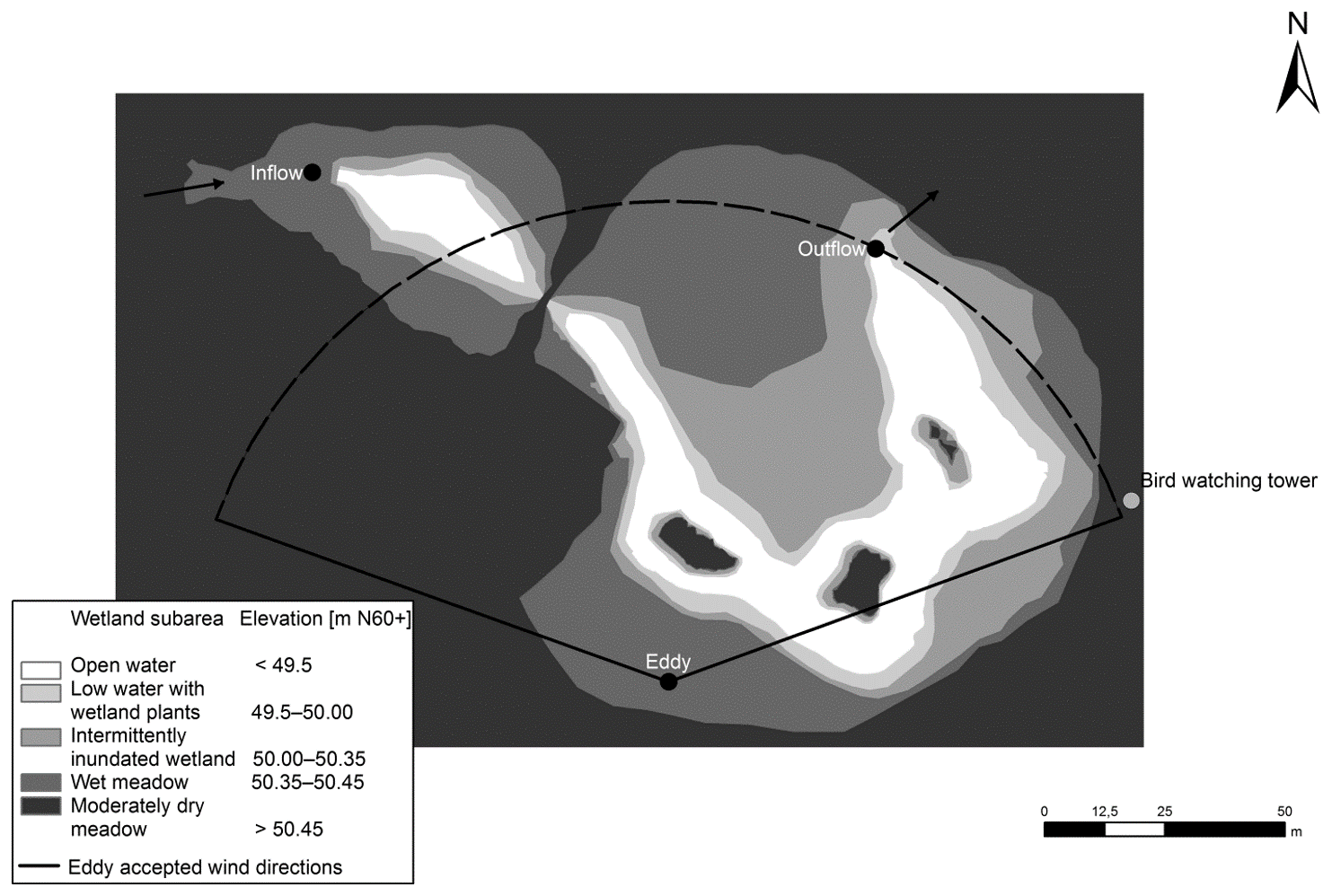
Figure 1The landscape classification of the Nummela wetland. Wetland subareas specified according to mean water level are shown with different colours. The arrows indicate the direction of the water flow. The black dots indicate the inflow and outflow measuring stations and the location of the EC tower.

Download

2.2 Water and micrometeorological measurements

Water monitoring stations were set up at the inlet (60.3283^∘ N, 24.3356^∘ E) and at the outlet (60.3281^∘ N, 24.3377^∘ E) of the wetland. During the 2012–2013 and 2013–2014 monitoring periods, water temperature as well as water turbidity, oxygen concentration, conductivity and pH were measured at the inlet and outlet monitoring station with the YSI-6600 series multiparameter sonde (YSI Inc., Yellow Springs, OH, USA). Measurements were conducted continuously with a 10 min interval. Water level at the outlet was measured continuously with a pressure gauge (STS Sensor Technik Sirnach AG, Switzerland). At the outlet monitoring station, the concentrations of dissolved carbon dioxide ([CO₂]) and dissolved methane ([CH₄]) were measured with Contros HydroC™ CO₂ and HydroC™ CH₄ sensors (CONTROS Systems and Solutions GmbH, Germany). In 2014, the same sensors were also installed at the inlet monitoring station to measure [CO₂] and [CH₄]. Dissolved CO₂ and CH₄ molecules diffuse from the water column into the detection chamber through a thin-film composite membrane where the concentration of CO₂ and CH₄ is determined by means of IR absorption spectrometry and Tunable Diode Laser Absorption Spectroscopy, respectively. NO₃-N and total phosphorus (TP) data have been previously published in Wahlroos et al. (2015). Briefly, NO₃-N was measured with Scan sensors (Scan GmbH, Austria) and TP was estimated based on turbidity data measured at 10 min intervals.

Local weather conditions were recorded with a Vaisala WXT weather transmitter (WXT520, Vaisala Oyj, Finland) at the inlet monitoring station. Rainfall, wind speed and direction, temperature, and relative humidity were recorded continuously at a 10 min interval. Photosynthetic photon flux density (PPFD) was measured with a PQS1 PAR quantum sensor (Kipp & Zonen, the Netherlands). Due to instrument failure we obtained PPFD data only from 26 January to 7 April and from 22 July to 29 December 2013. The gaps were filled with PPFD data from another meteorological station nearby (60^∘38^′ N, 23^∘58^′ E) in Lettosuo, Finland. The prevailing wind directions were southwest and northeast, and the average of half-hourly average wind speed was 1.13 m s⁻¹ from January to December 2013 with higher wind speed in winter than in summer. The average daily air temperature was 5.9^∘, with the minimum and maximum daily temperatures of −24.4 and 23.3^∘ in 2013. During the winter 2012–2013, there was ice coverage from the beginning of December 2012 to the end of March 2013. In contrast, winter was mild and warm in 2014, and there was practically no snow cover during a winter period (December 2013–March 2014).

2.3 Greenhouse gas measurements by the EC tower technique and gap-filling procedure

To understand the whole-ecosystem exchange of CO₂ and CH₄ in the wetland, a 2.9 m eddy covariance tower was established in the autumn of 2012 on the southern side of the wetland. The operational period of the EC tower was the entire calendar year of 2013 (from 1 January to 31 December 2013) and the peak growing season in 2014 (from 1 June to 31 August 2014). The EC set-up included a 3D-sonic anemometer (uSonic-3, Metek, Elmshorn, Germany) to measure the three wind speed components and sonic temperature, a gas analyser (LI-7200, LI-COR Inc., Lincoln, Nebraska, USA) which measures CO₂ and H₂O mixing ratio, and a TDL gas analyser (TGA100A, Campbell Scientific Inc., USA) to measure CH₄ mixing ratio. Data from the analysers were collected on a computer at the frequency of 10 Hz. The post-processing of the EC flux data has been done with EddyUH post-processing software (Mammarella et al., 2016). The fluxes were calculated as 30 min covariances between the vertical wind velocity and the gas mixing ratio using block averaging. The raw data were despiked according to standard methods (Vickers and Mahrt, 1997). Coordinate rotations were conducted by performing a two-step rotation to make the x axis along the mean wind direction and the mean vertical wind velocity zero within each 30 min block. The time lag between the anemometer and gas analyser signals, resulting from the transport through the inlet tube, was determined for each 30 min interval by maximizing the cross-correlation function between vertical wind speed and the scalar (CO₂ and CH₄). The fluxes were corrected for high-frequency loss due to the limited frequency response of the EC system and low-frequency loss due to the limited averaging time period used for calculating the fluxes. Theoretically and experimentally determined co-spectral transfer functions at low and high frequency were used in the correction (Mammarella et al., 2009).

After calculating the fluxes, data collected from periods when the sonic anemometer showed signs of freezing (mean temperature <0.5 ^∘C and standard deviation of temperature >1.5 ^∘) were discarded. The data collected during weak turbulence with friction velocity below 0.1 m s⁻¹ have been removed. The measurement points with flux stationarity greater than 1 were omitted to ensure the quality of the co-variances. Fluxes were further filtered according to the wind direction. Since the patchy forest to the southeast of the EC tower (from 100 to 200^∘) and the highway to the west (from 200 to 280^∘) could potentially lead to flow distortion and an additional source of CO₂ and CH₄, only fluxes from 280 to 100^∘ were accepted for further analysis. The percentage of 30 min fluxes excluded from this analysis was 72 % for CO₂ and 73 % for CH₄ in 2013, whereas in 2014 the percentage for data exclusion was 54 % for CO₂ and 68 % for CH₄.

We used an artificial neural network (ANN) technique to gap-fill half-hourly flux data using meteorological variables (Moffat et al., 2007; Papale et al., 2006). Those variables included radiation, air temperature, water temperature, water level, wind speed, relative humidity, time of the day, season, and dissolved CO₂ and CH₄ concentration in the water. We tested the model performance with different ANN architectures, starting from the architecture with the most complexity, and then reduced the variables to find the simplest ANN architecture with good performance (more than 5 % loss in model accuracy with additional variable reduction). For CO₂, water level and wind speed were found to have trivial contributions to the ANN model, and thus they were removed from the model input, while for CH₄, only wind speed was removed for the same reason. We found that dissolved gas concentrations greatly improved the model prediction as they captured the variation of diffusive fluxes from the water (Fig. S1 in the Supplement). Ancillary meteorological variables in general had good data coverage, and short gaps (up to several hours) were gap-filled by linear interpolation. The only exception was dissolved gas concentration, which had a long measurement breakage in 2013 (day of year 214–254). Fluxes were therefore gap-filled with two separate ANNs, one with dissolved gas concentration and one without. During the above-mentioned period with long gaps, the ANNs modelled without dissolved gas concentration were used to gap-fill the half-hourly flux data.

The Levenberg–Marquardt algorithm was used in the learning process of ANN. The optimized number of neurons in the hidden layer was determined by training the network 100 times with varying number of neurons (from 3 to 15), and 10 neurons were considered to be sufficient after evaluating the performance of the network using root-mean-square error (RMSE) (data not shown). The entire dataset was divided into three parts: two-thirds of the data were used to train the networks, one-sixth were used for testing the networks and the remaining one-sixth were used for validating the networks. Since the training of the networks can be biased towards periods with greater data coverage (e.g. daytime conditions), the environmental variables were first divided into five natural clusters using a k-mean clustering algorithm in MATLAB (MathWorks, Inc., Natick, MA, USA), and then the data used for training, testing and validation were proportionally extracted from each cluster. After each data extraction, the network was reinitialized for 10 times to avoid local minima, the initialization with the lowest RMSE was selected and the resulting network was saved. We repeated the whole process of data extraction and initialization for 20 times, and we used the median of these 20 predictions to gap-fill the missing flux values. The uncertainty of the ANN gap-filling procedure was presented using a 95 % confidence interval of the 20 ANN predictions.

In order to be confident in our gap-filling results, we also applied alternative gap-filling methods to EC fluxes using parameterization based on biological principles (see Supplement). The results on annual cumulative fluxes were not significantly different from the ones gap-filled using ANN; thus we only report the results from ANN in the following text.

2.4 Diffusive gas exchange

We calculated diffusive gas exchange F from open water according to the boundary layer model:

where k is the gas transfer velocity (cm h⁻¹), c_aq is the gas concentration in surface water (mol m⁻³) and c_eq is the gas concentration that surface water would have when it reaches equilibrium with the air (mol m⁻³). c_aq and c_eq can be obtained according to the solubility of the gas:

where k_H is Henry's law constant for the respective gas (mol L⁻¹ atm⁻¹), p is air pressure (atm), χ_water is the gas mixing ratio in surface water (ppm) and χ_air is the gas mixing ratio in the air (ppm). In this study, χ_water was obtained from the outlet monitoring station as it was located most of the time in the flux footprint area and it had longer data coverage than from the inlet monitoring station. The gas transfer velocity k can be calculated as the formula below (Cole and Caraco, 1998):

where U₁₀ is the horizontal wind speed extrapolated to 10 m using the theoretical log wind profile equation (m s⁻¹, approximately U₁₀=1.15U, where U is the measured wind speed at 2.9 m height in the study site) and Sc is the temperature-dependent Schmidt number of the respective gas. When a gas concentration measurement was not available, linear interpolation was applied to obtain monthly and annual diffusive GHG fluxes from the open water.

Although the above-mentioned Cole–Caraco (CC) method is the most simple and most often used model for gas transfer velocity, the limitation of the CC method is that it considers wind as the sole factor to cause the water turbulence and to drive the gas exchange. More complicated models were suggested to include the effect of buoyancy-flux-driven turbulence (Heiskanen et al., 2014; Tedford et al., 2014), which could not be applied in the current study as we did not have the measurements of some of the required model inputs, e.g. the net shortwave and longwave radiation from the water body. However, we believe that the CC method is suitable to be applied here. First, the water body in our study is located in an open area where the contribution of wind shear to the turbulence in the surface mixed layer is relatively high. During the study period in 2013, the average wind speed was 1.57 m s⁻¹ with a maximum of 7.1 m s⁻¹. Secondly, the k₆₀₀ estimated in our study was on average 0.66 m d⁻¹, well situated within the range of the k₆₀₀ which was directly measured by a floating chamber or gas tracer for small lakes and ponds (Holgerson et al., 2017). Thirdly, the estimated air–water fluxes of CH₄ and CO₂ based on the CC model were also well within the range of the diffusive gas fluxes over small lakes from other studies (Erkkilä et al., 2018; Mammarella et al., 2015). Finally, the parameterization of Cole and Caraco has been similarly applied to connected small open-water pools, and good agreement between the model estimation and the measurements was found (Cole et al., 2010; McNicol et al., 2017). Therefore, we decided to use the CC model to estimate diffusive fluxes from the water, bearing in mind that the calculated fluxes could potentially be underestimated.

2.5 Estimating zone fluxes and radiative forcing

By combining the EC tower and diffusive flux from the open water, the following model can be derived:

where F_EC is the flux measured by the EC tower, and F_water and F_veg stand for the fluxes from open-water and vegetated areas, respectively. f_water and f_veg are the footprint-weighted spatial fraction of open-water and vegetated areas. In this study, ebullition was neither measured nor calculated, so the flux from water was only represented by the diffusive flux.

Specifically, we first modelled the half-hourly flux footprint with a parameterization of a three-dimensional backward Lagrangian footprint model (Kljun et al., 2015) in MATLAB. Periods in which the wind came from the patchy forest to the southeast of the EC tower (between 100 and 200^∘) and the highway to the west (between 200 and 280^∘) were eliminated in the footprint analysis. Secondly, a land cover classification map of vegetated and open-water zones was delineated manually using a high-resolution aerial image (data from the National Land Survey of Finland Topographic Database 06/2013) with an image manipulation software (Gimp 2.10.6, https://www.gimp.org, last access: 22 November 2018). Thirdly, the flux footprints were aligned and combined with the land cover classification map to calculate half-hourly f_veg and f_water within 90 % footprint contour lines. Specifically, we assigned each footprint pixel within the 90 % footprint area to either open-water area or vegetated area on the land cover classification map while the footprint of the pixels outside the 90 % footprint area was regarded as zero. f_water was calculated as the sum of the footprint within the open-water area to the total footprints, while f_veg was calculated as the sum of footprint within the vegetated area to the total footprints. None of the 90 % footprint contour lines exceeded the map area, and the sum of f_veg and f_water equaled to 1. In order to obtain the long-term aggregated footprint of carbon fluxes, we calculated also the monthly and annual aggregated footprint climatology during the study period.

The uncertainty of the vegetation and water fraction comes from two sources. Firstly, the delineation of the distinct surface types was conducted based on a land surface map of the growing season in 2013, which neglected the change in the spatial extent of the vegetation throughout the presented GHG monitoring time. Secondly, although the footprint model used here is proven to be robust and general, there are uncertainties in the model predictions. To be more confident in the footprint estimation, it would be good to compare our results with footprint estimates based on large eddy simulations; however, that was out of the scope of the current study. With only one EC tower we could not cross-check the results as was done in another study (Matthes et al., 2014). However, we chose to follow a simple approach dividing the landscape into vegetation and open water because we did not observe significant vegetation expansion to cover more of the open water during the growing season in 2013, and thus the area of open water was relatively constant during the monitored time periods. Vegetation establishment at the Gateway wetland was very rapid in the first growing season, and by the summer 2012 emergent vegetation had densely established at the intended shallow wetland areas. Furthermore, the clear effect of the footprint-weighted fraction of open water on the synchronization between EC CH₄ measurements and diffusive CH₄ flux from water was nicely demonstrated in our analysis (Fig. S3).

To better understand the influence of greenhouse gas fluxes in this urban wetland, we calculated the sustained global warming potential (SGWP) for CO₂ and CH₄ over a 100-year horizon in each surface type. The difference between SGWP and global warming potential (GWP) is that SGWP accounts for the effect of GHG remaining in the atmosphere during the period. Since CH₄ is a more potent greenhouse gas, we multiply the emission of CH₄ by a factor of 45 to convert it to kg CO₂-eq m⁻² yr⁻¹ (Neubauer and Megonigal, 2015). However, for an easy comparison between our results and those from other studies using the conventional method, we calculated also CH₄ fluxes as CO₂ equivalents using a GWP of 34 following the Fifth Assessment Report of IPCC (2013).

2.6 Statistical analysis

Differences in the fluxes and environmental variables between the two peak growing seasons (summer 2013 and 2014) were evaluated using the t test. Cumulative annual GHG fluxes measured by the EC tower are reported as the median of the 20 ANN predictions, and uncertainty is presented as the 95 % confidence interval of the 20 ANN predictions. As diffusive GHG fluxes were calculated from gas concentration meteorological parameters, no standard error is reported for the cumulative annual fluxes from the open water. All statistical analyses were performed in MATLAB.

We also conducted wavelet coherence analysis to explore the temporal correlations between fluxes and environmental variables on the multi-temporal scales (Grinsted et al., 2004; Torrence and Webster, 1998). Since the fluxes are gap-filled using some of the environmental variables, simply applying the wavelet coherence analysis to all the variables can overstate the correlations. Therefore, we only conducted wavelet coherence analysis between gap-filled ecosystem flux time series and those independent environmental variables which were not used in the gap-filling procedure (concentration of NO₃-N and TP), while Pearson correlations (r) were determined between non-gap-filled fluxes and the other environmental variables.

3.1 Ecosystem seasonality and environmental variables

Daily average PPFD ranged from 0.9 to 691.5 µmol m⁻² s⁻¹ in 2013, with the highest value appearing in July. June had the highest monthly average PPFD with 486.1 µmol m⁻² s⁻¹, followed by July and August with 470.2 and 430.6 µmol m⁻² s⁻¹, respectively. The PPFD during the peak growing season in 2014 was on average 361.8 µmol m⁻² s⁻¹, which is lower than that during the same period in 2013 (Fig. 2a).

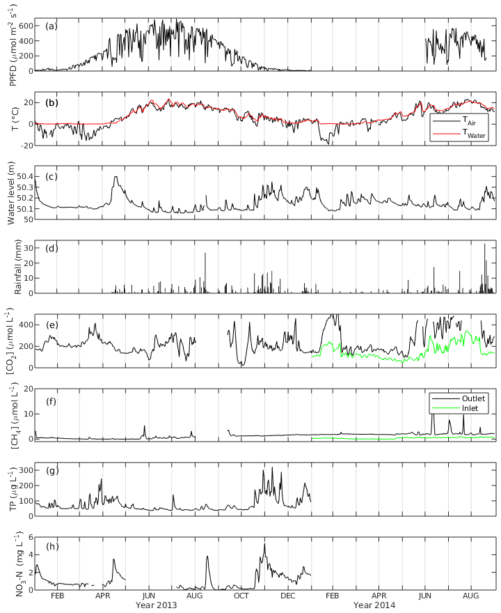
Figure 2The daily average of (a) photosynthetic photon flux density (PPFD), (b) air and water temperature (T_air and T_water), (c) water level, (d) rainfall, (e) CO₂ concentration ([CO₂]), (f) CH₄ concentration ([CH₄]), (g) concentration of total phosphorus (TP) and (h) concentration of NO₃-N of the Nummela wetland from January 2013 to August 2014.

Download

Mean daily water temperature (T_water) ranged from 0 ^∘C in March to 23.7 ^∘C in June with an annual average of 7.9 ^∘C in 2013 and from 0 ^∘C in February to 21.4 ^∘C in July in 2014. Mean daily air temperature (T_air) had more fluctuation and ranged from −15.6 ^∘C in January to 23.3 ^∘C in June 2013 and from −19.0 ^∘C in January to 23.4 ^∘C in July 2014 (Fig. 2b). The open-water area experienced an ice-covered period between 1 January and 31 March 2013, while the winter 2013–2014 was so mild and warm that there was practically no snow cover during December 2013–March 2014. Comparing the temperature between the two peak growing seasons, both T_water and T_air were higher in June 2013 while T_air was lower in July 2013 than in 2014. In August, there was no significant temperature difference between the 2 years. Four seasons were classified for the ecosystem based on the trend in T_air and T_water. In spring (April and May), the daily temperature started to increase, the vegetation showed a sign of early growing season and the warm temperature unfroze the lake. In summer, the peak growing season (June–August), vegetation exhibited the maximum growth, and the temperatures reached the annual maxima. In autumn (September and October), daily temperatures began to drop and the vegetation showed signs of early senescence. In winter (January to March and November and December), temperatures reached the annual minimum and vegetation was inactive in carbon sequestration. Precipitation was higher in August 2014 than in the preceding August, almost twice as high as that of 2013.

WL was higher in the winter and lower in the summer in 2013. The daily average of WL varied between 50.06 m in July 2013 and 50.4 m in April 2013. There was a spring peak in 2013 when the highest WL was observed due to snowmelt, while in 2014 no such event appeared due to the mild winter 2013–2014 without an ice-covered period (Fig. 2c). The average daily WL from January to August was similar (50.13 and 50.15 cm for 2013 and 2014, respectively). However, during the peak growing season, it was on average 5.7 cm higher in 2014 than in 2013.

The annual rainfall in 2013 (snowfall not included) was 363.6 mm, which happened mostly during summer and autumn (Fig. 2d). The maximum daily-averaged rainfall was in August (26.7 mm d⁻¹), while monthly-averaged rainfall was highest in November with 73.8 mm per month followed by August with 68.3 mm per month. In 2014, an exceptionally high amount of rainfall was observed in August (125.7 mm per month), while the amount of rainfall in the other months was similar to 2013.

The daily-averaged CO₂ concentration in the water ([CO₂]) in 2013 had large variation with the maximum (461 µmol L⁻¹) and the minimum (21.6 µmol L⁻¹) (Fig. 2e). [CO₂] was higher in 2014 with an average of 262.6 µmol L⁻¹ from January to August than in 2013 with an average of 211.5 µmol L⁻¹. It also exhibited seasonal variation with high concentration in summer (360.3 µmol L⁻¹) and low concentration in winter (223.4 µmol L⁻¹). The [CO₂] measured in the inflow was generally lower than that in the outflow, and they were well correlated (r=0.84). [CH₄] in the outflow was on average 5 times higher in 2014 than in 2013. The average annual concentration was 0.81 µmol L⁻¹ in 2013 and 2.25 µmol L⁻¹ in 2014. There were peak [CH₄] episodes in the outflow in May 2013 with a maximum of 5.43 µmol L⁻¹. During the summer months in 2014 there were even higher outflow [CH₄] peaks, with a maximum of 16.83 µmol L⁻¹. The [CH₄] had a mean of 0.42 µmol L⁻¹ in the inflow which was lower than that in the outflow, and there were no prominent [CH₄] peaks observed in the inflow. [CH₄] in the inflow and outflow were weakly correlated (r=0.2) (Fig. 2f).

The median concentration of total phosphorus (TP) measured at the outflow monitoring station was 56 µg L⁻¹, and the median NO₃-N concentration was 0.69 mg L⁻¹ in 2013 (Fig. 2g, h). In the annual perspective, TP and NO₃-N concentration consisted of several runoff peaks occurring after rain or snow melting events. This wetland serves as a nutrient removal measure as it improved water quality by retaining P and N from runoff before the release to the receiving lake, where the annual TP reduction was 10 % and NO₃-N reduction was 3 % from the original concentration in 2013 (Wahlroos, 2019).

3.2 Flux footprint mapping

A footprint distribution was modelled for each half hour when an eddy flux measurement was collected at the EC tower. The open-water area accounted for 10 % to 16 % of the total wetland area within the footprint, while the rest was comprised of wetland vegetation. When weighted with footprint distribution, f_water ranged from 0 % to 25.5 % and f_veg from 74.5 % to 100 %. The first quartile, median and third quartile of f_water were 0.09 %, 14.1 % and 17.9 %, respectively, and those of f_veg were 82.1 %, 85.9 % and 91.3 %, respectively.

The monthly cumulative footprint was slightly different for CO₂ and for CH₄ due to the different missing flux values. However, the difference on average was so small (7 %) and the footprint of CO₂ was used in further analysis. The flux footprints were shown to be northeast to the EC mast due to the wind direction filtering, meaning only half-hourly data with wind directions from the wetland area were considered in the analysis (Fig. S2). The monthly average of the 90 % footprint area covered a minimum of 0.69 ha to a maximum of 2.28 ha with a mean of 1.3 ha. The mean extent of the 90 % flux footprints was 128 m. After applying the flux footprint function, the monthly average of the footprint-weighted spatial fraction of open water showed lower value in summer and higher value in winter, ranging from 11.3 % to 21.4 % with a mean of 13.3 % in 2013. In 2014, during the peak growing season, on average 13.8 % of the wetland area was open water and the mean f_water was 10 %.

3.3 CO₂ and CH₄ fluxes

3.3.1 Ecosystem CO₂ and CH₄ fluxes

Ecosystem CO₂ and CH₄ fluxes measured by the EC tower showed the ecosystem was nearly CO₂ neutral and it was a small CH₄ source in 2013.

Daily average of NEE was near zero during winter time (January to March, on average 0.37 µmol C-CO₂ m⁻² s⁻¹), it was slightly positive in spring and it became negative from the end of May until the end of August, indicating the ecosystem was a CO₂ sink during this period, with a maximum negative value of −5.14 µmol C-CO₂ m⁻² s⁻¹ in June. Daily average NEE was highest in September with a maximum of 3.29 µmol C-CO₂ m⁻² s⁻¹. In October, November and December, NEE remained low but still positive (on average 0.77 g µmol C-CO₂ m⁻² s⁻¹), demonstrating the milder winter between 2013 and 2014 (Fig. 3). NEE exhibited strong seasonality in 2013, which was negative during June, July and August, meaning the ecosystem was a CO₂ sink while the rest of year it was a CO₂ source. NEE was lowest in June and highest in September. The cumulative NEE in 2013 was 8 g C-CO₂ m⁻² yr⁻¹, with the 95 % confidence interval between −18.9 and 34.9 g C-CO₂ m⁻² yr⁻¹ (Fig. 3).

Figure 3Daily average of net ecosystem exchange of CO₂ (NEE, µmol m⁻² s⁻¹) in 2013. Filled dots indicate measurement (when available half-hourly measurement data ≥10) and circles indicate gap-filled data (when available half-hourly measurement data <10). The insert shows cumulative NEE (g C m⁻²) in the ecosystem and the red line indicates the zero reference line. Error bounds (marked in grey) on cumulative NEE reflect the 95 % confidence interval for the gap-filling procedure.

Download

Daily-averaged CH₄ was low but not negligible from January to April (on average 5.1 nmol C-CH₄ m⁻² s⁻¹), with a sudden rise at the end of May reaching a maximum of 48.9 nmol C-CH₄ m⁻² s⁻¹. During summer months the ecosystem exhibited relatively high CH₄ emission (on average 15.4 nmol C-CH₄ m⁻² s⁻¹), which is not comparable with the emission episode in May but higher than winter months. In autumn (September and October) the daily-average CH₄ was 8.8 nmol C-CH₄ m⁻² s⁻¹, and after that it gradually decreased throughout the rest of the year with an average of 5.5 nmol C-CH₄ m⁻² s⁻¹. The cumulative CH₄ for 2013 was 3.9 g C-CH₄ m⁻² yr⁻¹, with the 95 % confidence interval between 3.75 and 4.07 g C-CH₄ m⁻² yr⁻¹ (Fig. 4).

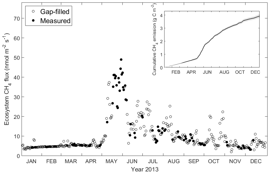
Figure 4Daily average of ecosystem CH₄ flux measured by the EC tower and cumulative CH₄ emission in 2013. Filled dots indicate measurement (when available half-hourly measurement data ≥10) and circles indicate gap-filled data (when available half-hourly measurement data <10). The insert shows cumulative CH₄ emission, with the error bounds in grey reflecting the 95 % confidence interval for the gap-filling procedure.

Download

Comparing the peak growing season between 2013 and 2014, the 30 min NEE ranged from −20.0 µmol C-CO₂ m⁻² s⁻¹ in June to 18.5 µmol C-CO₂ m⁻² s⁻¹ in September 2013. During the peak growing season 2014, NEE had the lowest value of −22.6 µmol C-CO₂ m⁻² s⁻¹ in June. The monthly NEEs of the peak growing season were −84.1, −76.1 and −22.2 g C-CO₂ m⁻² per month in June, July and August 2013, and they were −97.6, −47.5 and −19.6 g C-CO₂ m⁻² per month in 2014. The average CH₄ emissions in June, July and August were 24.4, 10.8 and 11 nmol m⁻² s⁻¹ in 2013, and they were 15.5, 21.3 and 21.3 nmol m⁻² s⁻¹ in 2014, respectively.

3.3.2 Diffusive CO₂ and CH₄ fluxes from the open-water area

Diffusive CO₂ and CH₄ fluxes from the open water were estimated based on wind speed, [CO₂] and [CH₄] (see Sect. 2.4). The variation of diffusive fluxes demonstrated a pattern driven by both wind speed in the short term and gas concentration dynamics in the water in the long term. Diffusive CO₂ fluxes ranged from −0.07 to 4.09 µmol CO₂ m⁻² s⁻¹ with a mean of 1.04 µmol CO₂ m⁻² s⁻¹ in 2013, indicating CO₂ oversaturation in the water. From June to September the averaged flux (1.27 µmol CO₂ m⁻² s⁻¹) was higher than that of the other months (Fig. 5a), corresponding to the higher [CO₂] in the water during summer months (Fig. 2e). The monthly-averaged diffusive CO₂ flux during peak growing season in 2014 was 2.34, 2.71 and 1.99 µmol CO₂ m⁻² s⁻¹ for June, July and August, which is significantly higher than during the same period in 2013 due to the high [CO₂] in the open water (Fig. 2e).

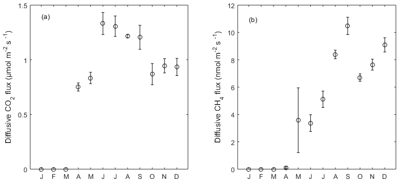
Figure 5Monthly average of (a) diffusive CO₂ and (b) CH₄ flux from the open water in 2013. Error bar indicates the standard error of the mean. From January to March there was an ice-covered period.

Download

The average diffusive CH₄ emissions in 2013 was 4.9 nmol C-CH₄ m⁻² s⁻¹, where a peak emission appeared in late May with the highest flux of 137.6 nmol C-CH₄ m⁻² s⁻¹. Monthly-averaged CH₄ diffusive fluxes showed an increasing trend towards the end of the year with large variation in May due to the peak concentration episode. This phenomenon was mainly driven by the increasing dissolved CH₄ concentration in the outflow in 2013. The monthly-averaged diffusive CH₄ flux during peak growing season in 2014 was 20.9, 18.9 and 13.5 nmol CH₄ m⁻² s⁻¹ for June, July and August, respectively, and they were significantly higher than the same period in 2013 due to the high [CH₄] in the open water (Fig. 2f).

3.3.3 Diel patterns in CO₂ and CH₄ fluxes

Only non-gap-filled data were used for determination of diel patterns in both gas fluxes. CO₂ and CH₄ fluxes from the vegetated areas (F_veg) were calculated for each 30 min interval according to Eq. (5). As expected, CO₂ flux showed a strong diel pattern in summer with CO₂ uptake during daytime and release in the night, which was controlled by photosynthetic activity (Fig. 6a). The summer peak CO₂ uptake reached 11.5 µmol m⁻² s⁻¹ for the whole constructed wetland ecosystem and 15.2 µmol m⁻² s⁻¹ for the vegetated areas. The CO₂ flux from the vegetated areas had higher maximum uptake than the EC measurements carried out over the whole constructed wetland. In the winter, the CO₂ fluxes from both tower and vegetation were similar, being on average 0.46 and 0.55 µmol m⁻² s⁻¹ respectively (Fig. 6b).

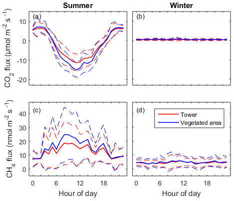
Figure 6Mean diel pattern of the half-hourly net CO₂ and CH₄ fluxes in summer (a, c) and in winter (b, d). The dashed lines represent the standard deviation. Red lines indicate measurement from the EC tower and the blue lines show the fluxes modelled for the vegetated area.

Download

CH₄ flux also showed diel patterns in the summer with much larger variability than those from CO₂ flux. CH₄ emission in general was higher in daytime than in nighttime. In the daytime in summer, CH₄ flux from the vegetated area was higher than the flux measured from the tower while there was no difference during the nighttime (Fig. 6c, d). The summer peak daytime flux from the tower (18.9 nmol m⁻² s⁻¹) and the vegetated area (24.7 nmol m⁻² s⁻¹) was 2.4 times and 3.3 times higher than the nighttime flux (7.5 nmol m⁻² s⁻¹), respectively. This can be understood as daytime CH₄ flux being linked with photosynthesis while nighttime CH₄ flux is controlled by other processes like diffusion, ebullition and convection between the soil, water and atmosphere. In winter there was a small (on average 4.6 nmol m⁻² s⁻¹) but constantly positive CH₄ flux without an obvious diel pattern.

3.4 Environmental variables with fluxes

Only non-gap-filled flux data were used in the Pearson correlation analysis between environmental variables and flux pairs. Radiation, T_air and T_water all had a high negative correlation coefficient (r) with NEE and a high positive r with CH₄ flux in 2013, corresponding to the results of ANN model parameter selection. Radiation was best correlated with NEE and T_water was best correlated with CH₄ (Table 1). The correlations were rather weak (small r or even the opposite sign of r) during 2014 due to the short measuring period and narrow ranges of the variables. Water level was positively correlated with NEE and negatively correlated with CH₄, which was counter-intuitive, possibly because it was masked by temperature variation as the water level was in general higher in winter and lower in summer. [CO₂] and [CH₄] were not correlated with either NEE or CH₄, although they were shown to be important parameters in ANN model selection.

NO₃-N did not show consistent correlation with any of the fluxes (Fig. 7a, b). The variation of TP was negatively leading the change in NEE at 1 d scale (more TP leads to more CO₂ uptake; Fig. 7c) where the time lag varies between 1 and 5 h (data not shown). TP had a positive correlation with CH₄ flux (more TP leads to more CH₄ emission) at 1 d scale (Fig. 7d) and TP led the CH₄ flux by ∼2 h (data not shown).

Table 1Pearson correlation coefficient (r) between the daily averages of environmental variables and fluxes in 2013 and 2014. NEE – net ecosystem exchange; T_air – air temperature; T_water – water temperature; PPFD – photosynthetic photon flux density; WL – water level; [CO₂] and [CH₄] – CO₂ and CH₄ concentration measured in the outlet; ^* indicates only peak growing seasons (June, July and August) are included in the analysis.

Download Print Version | Download XLSX

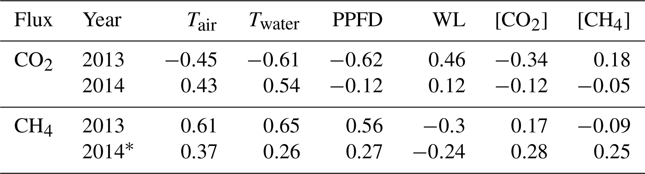
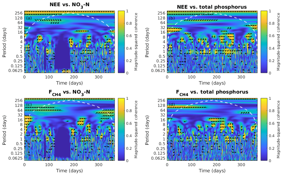
Figure 7Wavelet coherence analysis and the phase difference between ecosystem fluxes, the net ecosystem exchange (NEE) and the CH₄ flux ($F_{{\mathrm{CH}}_{\mathrm{4}}}$), and nutrient concentration in the water, NO₃-N and total phosphorus from January to December 2013. The colour represents the power of the coherence from 0 to 1. The phase difference is indicated by black arrows which only show up where the coherence is greater than or equal to 0.5. Rightwards arrow (→) indicates in-phase (two time series in synchrony) and arrows in other direction indicate out of phase (representing lags between time series); i.e. leftwards arrow (←) indicates anti-phase, downwards arrow (↓) indicates the first series (fluxes) leads by quarter cycle and upwards arrow (↑) indicates the second series (NO₃-N and total phosphorus) leads by quarter cycle. White dash contour lines indicate the cone of influence.

Download

3.5 Estimating radiative forcing from different zones

To obtain the climate forcings from each land surface type, we calculated the annual cumulative fluxes from the vegetated area based on Eq. (5) using footprint-weighted spatial fraction, ecosystem fluxes and diffusive fluxes from the open water (see Sect. 2.5). The annual median value of footprint-weighted spatial extent was used to calculate the annual fluxes, which showed the open-water area was a CO₂ source (297.5 g C-CO₂ m⁻² yr⁻¹) and the vegetated area was a CO₂ sink (−39.5 C-CO₂ m⁻² yr⁻¹). Both the open-water area and the vegetated area were CH₄ sources, but the CH₄ emission from the vegetated area was higher than the open-water area, being 4.26 and 1.73 g C-CO₂ m⁻² yr⁻¹, respectively (Table 2).

Table 2Annual CO₂ and CH₄ exchange, their sustained global warming potential (SGWP) and global warming potential (GWP) from different surface zones in the Nummela wetland in 2013. “Ecosystem”, “water” and “vegetation” represent flux, SGWP and GWP measured or calculated from the ecosystem by the EC tower, from the open-water and vegetated areas, respectively. The numbers in the square bracket represent the 95 % confidence interval of the average. No error bounds are reported for flux, SGWP and GWP from open water as they are modelled using gas concentration in the water and meteorological measurements.

Download Print Version | Download XLSX

Open water has contributed a large amount of CO₂ emission into the atmosphere through diffusion (1.09 kg CO₂-eq m⁻² yr⁻¹), whereas the CH₄ emission was relatively small (0.104 kg CO₂-eq m⁻² yr⁻¹). The vegetated area was a small sink of CO₂ but the cooling effect of vegetation by CO₂ uptake was relatively small (−0.145 kg CO₂-eq m⁻² yr⁻¹) compared to its CH₄ emission (0.256 kg CO₂-eq m⁻² yr⁻¹). Overall, the ecosystem had a small warming effect of 0.263 kg CO₂-eq m⁻² yr⁻¹, of which 89 % was contributed by CH₄ (Table 2).

4.1 The GHG fluxes from an urban storm water wetland ecosystem

The studied urban wetland ecosystem was a small carbon source over the full-year studied period in 2013. Due to the scarcity of studies on urban wetlands using the EC method, we compare our results to restored wetlands which can be considered to be proxy ecosystems to urban wetlands, with both including wetting practice in an ecosystem which has been drained or dry previously. The annual CO₂ balance of 8 g C-CO₂ m⁻² yr⁻¹ from the ecosystem, or −39.5 g C-CO₂ m⁻² yr⁻¹ from the vegetated area (Table 2), was small compared to a restored wetland in western Denmark where the annual CO₂ balance ranged from −286 to −53 g C-CO₂ m⁻² yr⁻¹ (Herbst et al., 2013), and the annual CH₄ balance of 3.9 g C-CH₄ m⁻² yr⁻¹ was less than half of the annual CH₄ emission (between 9 and 13 g C-CH₄ m⁻² yr⁻¹) in that study. Over a network of restored freshwater wetlands in California, the CO₂ sequestration can be up to nearly 700 g C m⁻² yr⁻¹ and CH₄ emission up to 63 g C m⁻² yr⁻¹ (Hemes et al., 2018). It is not surprising that the studied ecosystem appeared to be CO₂ neutral as it was recently constructed. The herbaceous vegetation has been allowed to fully self-establish without human intervention, and at the early successional stage, plant diversity and biomass were still increasing each year (Wahlroos, 2019). With the vegetation being more developed, a greater CO₂ uptake from the vegetated area can be expected in the following years. The low CH₄ emission observed in this study may be due to the depletion of organic matter in the bottom soil from agricultural uses; thus it provided little substrate for anaerobic microbial activity to produce CH₄. With the accumulation of organic matter in the anoxic wetland sediment, CH₄ production may increase in the future. Certain chemical compounds like Fe in mineral soils can also inhibit CH₄ production, leading to much-lower ecosystem-scale CH₄ flux (Chamberlain et al., 2018). In the meantime, methane-oxidizing bacteria (methanotroph) regulate CH₄ consumption at the soil–water interface. With the ecosystem being used previously as cropland, the physical disturbance of soil may have greatly reduced the methanotroph communities so that the CH₄ oxidation may also be low in the soil (Smith et al., 2000; Saggar et al., 2008). Furthermore, after the initial establishing phase, the ecosystem productivity can also be reduced at a water treatment wetland due to the standing litter that inhibits the generation of new vegetation growth. It was shown that in a restored freshwater wetland the ecosystem was a net CO₂ sink ($-\mathrm{804}\pm \mathrm{131}$ g C-CO₂ m⁻² yr⁻¹) in 2002–2003, 6 years after the restoration, but nearly CO₂ neutral in 2010–2011 due to the reduced photosynthetic plants (Anderson et al., 2016). Thus, given the urban wetland is sustained for a sufficiently long period, it is still unclear whether the CO₂ uptake from the vegetated zone would compensate for its CH₄ emission, not considering the large GHG emission from the open-water zone. Thus, similar studies as the present one should be conducted at a later stage after the construction of the wetland to fully reveal the GHG balance of the ecosystem over time.

Overall, the ecosystem CO₂ and CH₄ fluxes measured by the EC tower ranged from −5.33 to 3.4 g C-CO₂ m⁻² d⁻¹ and from 1.0 to 55.2 mg C-CH₄ m⁻² d⁻¹, respectively. They are consistent with the flux ranges provided by other studies on GHG fluxes in restored wetlands (Anderson et al., 2016; Knox et al., 2015; Matthes et al., 2014; Morin et al., 2014b; Herbst et al., 2013), although for both gases they tend to be on the lower end. NEE exhibited seasonal variation so that the ecosystem was a CO₂ sink between June and August. The highest NEE appeared in September possibly because photosynthesis greatly reduced due to plant senescence while ecosystem respiration remained relatively high because of the warm temperature. Previous studies have found good agreement between CH₄ emission and photosynthesis as plants provide substrates for methanogenesis (Rinne et al., 2018), which was not observed in the daily average of gas fluxes in this study (Figs. 2 and 3) as the peak CH₄ flux appeared in May and peak gross primary productivity appeared in July (data now shown). Nonetheless, both CH₄ and CO₂ fluxes, especially those obtained from the vegetated areas, exhibited strong diurnal cycles during summer with synchronized peaks around noon (Fig. 6a, c). This finding reflects that short-term CH₄ emission from vegetation is linked with photosynthesis by providing labile carbon from root exudate and by gas transport through aerenchyma and open stomata, while long-term CH₄ emission may be determined by complex processes related to environmental variables, e.g. temperature and redox potential (Linden et al., 2014).

4.2 Parsing GHG fluxes from heterogeneous land surfaces

We found that the open-water area was constantly a source of CO₂ and CH₄ to the atmosphere during the studied period as the [CO₂] and [CH₄] in the water generally exceeded the atmosphere equilibrium except during the ice-covered period (Fig. 5). The annual average of [CO₂] in the surface water in 2013 was 0.3 % in our study, comparable to 0.4 % in another temperate restored wetland (McNicol et al., 2017), while the seasonal pattern (higher in summer and fall) was the opposite of what McNicol et al. (2017) found. We also found that both [CO₂] and [CH₄] were higher in 2014 than 2013 (Figs. 2d, 1e). The O₂ concentration ([O₂]) and O₂ balance ([O₂]_outlet − [O₂]_inlet) measured by another study on the same wetland (Wahlroos, 2019) could partially explain the observed phenomenon. The relatively high water temperature and oxic conditions in the water in fall 2013 have allowed high decomposition of detritus leading to high [CO₂] (Wahlroos, 2019). The long period of hypoxia during summer 2014 could explain the 3-fold increase in [CH₄] as the condition was more favourable for CH₄ production. The negative O₂ balance in summer 2014 indicated strong O₂ consumption by microbial decomposition producing CO₂ in the water. As the long-term diffusive fluxes (daily and monthly) were mainly driven by gas concentration in the water, it was straightforward to understand high diffusive CO₂ and CH₄ fluxes in 2014 compared to 2013. Interestingly, the ecosystem CH₄ emission in 2013 was well synchronized with the diffusive CH₄ flux by capturing sporadic emission episodes from the water (Fig. S3a, c), while they were not synchronized in summer 2014 although several stronger diffusive peaks happened (Fig. S3b, d). When footprint-weighted contribution was accounted for, it clearly revealed that the synchronization of CH₄ emission from ecosystem and water was closely related to the flux footprint distribution. When there was high flux contribution from the open water (20 %–25 %), high diffusive CH₄ was also reflected in ecosystem flux measured by EC. This has further proved the application of footprint analysis is essential in explaining gas exchange from heterogeneous surfaces using EC data.

It is worth noting that in our study we only classified the surface landscapes into “open water” and “vegetation” but neglected the difference in sink/source strength from different plant types within the vegetation zone (Fig. 1). We did not account for the dissimilarity between vegetation types because the characteristics in gas exchange are much more distinct between open water and vegetation, which was the focus of this study. For the same reason, ebullition was not considered in this study either, as ebullition was shown to have only minor significance in a restored wetland, accounting for less than 0.1 % of ecosystem CO₂ flux and 4.1 % of ecosystem CH₄ flux (McNicol et al., 2017). However, for a proper downscaling analysis of EC data, the subareas of different plant types and ebullition should also be taken into account.

4.3 Climate impact of urban wetland and implications for management

In the present study, the urban boreal wetland had an overall SGWP of 0.263 kg CO₂-eq m⁻² yr⁻¹ which was comparable to or higher than other restored wetlands in the boreal region (Herbst et al., 2013) and within the range of inter-annual variation or lower than restored wetlands in the temperate zone (McNicol et al., 2017; Anderson et al., 2016). Different from other studies, the urban wetland was CO₂ neutral and a CH₄ source. It is worth noting that the paramount contribution of CH₄ in ecosystem SGWP was mainly driven by the large footprint-weighted spatial area of the vegetation (see Sect. 3.2). In fact, The SGWP of GHG emission from open water (1.194 kg CO₂-eq m⁻² yr⁻¹) was 10 times as large as that from vegetation (0.111 kg CO₂-eq m⁻² yr⁻¹) (Table 2). The implication of this result is that, during wetland restoration, it would be more beneficial to have large patches of emergent vegetation at least from the GHG emission point of view. Similar results have been obtained by other studies as well, indicating that open water has more climate-warming impact than emergent vegetation due to the large diffusive fluxes from open water (Stefanik and Mitsch, 2014; McNicol et al., 2017). The climate impact of natural wetland depends on the net balance between the cooling effect of CO₂ uptake by vegetation and the warming effect of other GHG emissions, mainly CH₄ (Bridgham et al., 2013). In wetlands constructed in urban areas, the extent of open water, which is a significant emitter of CO₂, should also be taken into consideration when evaluating the role of urban wetland in global climate change.

Our results also showed that total phosphorus enhanced both CO₂ uptake and CH₄ emission, which have contradictory climate impacts to the ecosystem (Fig. 7b, d). Although it is out of the scope of our study, it would be very interesting to understand the mechanisms and quantify the magnitude and the duration of these enhancements induced by nutrient input. Previous studies have found that nutrient inputs can influence the identity of the key primary producer (submerged plants versus phytoplankton) in the water, which is crucial in shaping the CH₄ emission from shallow water (West et al., 2016; Davidson et al., 2018). Submerged plants may decrease CH₄ production in the lake by transporting oxygen to the sediment and providing good habitat for CH₄-oxidizing bacteria (Heilman and Carlton, 2001), while phytoplankton was shown to significantly increase CH₄ ebullition by changing the quality of the dissolved organic carbon which promotes methanogenesis (West et al., 2016) and/or by altering the sediment texture and redox conditions favouring the release of bubbles. As a result, we suggest controlling the nutrient input to the water of the newly established wetland to limit the abundance of phytoplankton as well as to support the existence of submerged plants.