Dissolved CH<sub>4</sub> coupled to photosynthetic picoeukaryotes in oxic waters and to cumulative chlorophyll <i>a</i> in anoxic waters of reservoirs

León-Palmero, Elizabeth; Contreras-Ruiz, Alba; Sierra, Ana; Morales-Baquero, Rafael; Reche, Isabel

doi:https://doi.org/10.5194/bg-17-3223-2020

Articles | Volume 17, issue 12

https://doi.org/10.5194/bg-17-3223-2020

Articles | Volume 17, issue 12

Research article

26 Jun 2020

Research article |

| 26 Jun 2020

Dissolved CH₄ coupled to photosynthetic picoeukaryotes in oxic waters and to cumulative chlorophyll a in anoxic waters of reservoirs

Elizabeth León-Palmero, Alba Contreras-Ruiz, Ana Sierra, Rafael Morales-Baquero, and Isabel Reche

Abstract

Methane (CH₄) emissions from reservoirs are responsible for most of the atmospheric climatic forcing of these aquatic ecosystems, comparable to emissions from paddies or biomass burning. Primarily, CH₄ is produced during the anaerobic mineralization of organic carbon in anoxic sediments by methanogenic archaea. However, the origin of the recurrent and ubiquitous CH₄ supersaturation in oxic waters (i.e., the methane paradox) is still controversial. Here, we determined the dissolved CH₄ concentration in the water column of 12 reservoirs during summer stratification and winter mixing to explore CH₄ sources in oxic waters. Reservoir sizes ranged from 1.18 to 26.13 km². We found that dissolved CH₄ in the water column varied by up to 4 orders of magnitude (0.02–213.64 µmol L⁻¹), and all oxic depths were consistently supersaturated in both periods. Phytoplanktonic sources appear to determine the concentration of CH₄ in these reservoirs primarily. In anoxic waters, the depth-cumulative chlorophyll a concentration, a proxy for the phytoplanktonic biomass exported to sediments, was correlated to CH₄ concentration. In oxic waters, the photosynthetic picoeukaryotes' abundance was significantly correlated to the dissolved CH₄ concentration during both the stratification and the mixing. The mean depth of the reservoirs, as a surrogate of the vertical CH₄ transport from sediment to the oxic waters, also contributed notably to the CH₄ concentration in oxic waters. Our findings suggest that photosynthetic picoeukaryotes can play a significant role in determining CH₄ concentration in oxic waters, although their role as CH₄ sources to explain the methane paradox has been poorly explored.

Please read the corrigendum first before continuing.

Download & links

Article (PDF, 4667 KB)

Notice on corrigendum
The requested paper has a corresponding corrigendum published. Please read the corrigendum first before downloading the article.
Article (4667 KB)

Corrigendum
Supplement (8918 KB)

Download & links

The requested paper has a corresponding corrigendum published. Please read the corrigendum first before downloading the article.

Article (4667 KB)
Corrigendum
Supplement (8918 KB)
BibTeX
EndNote

How to cite

How to cite.

Dates

Received: 22 Jan 2020 – Discussion started: 04 Feb 2020 – Revised: 09 Apr 2020 – Accepted: 16 Apr 2020 – Published: 26 Jun 2020

1 Introduction

Lakes and reservoirs are significant sources of methane (CH₄), affecting the atmospheric climatic forcing (Deemer et al., 2016). The estimated contribution of lakes to the global emission budget is ca. 71.6 Tg CH₄ yr⁻¹ (Bastviken et al., 2011), and the specific contribution of reservoirs ranges between 4 and 70 Tg CH₄ yr⁻¹, representing up to 10 % of total CH₄ emissions (Deemer et al., 2016). Although freshwater only covers about 5 %–8 % of the Earth's surface (Mitsch et al., 2012), it emits more CH₄ than the ocean surface (Saunois et al., 2016). Traditionally, the net CH₄ production is determined by archaeal methanogenesis, which produces methane as an end product of organic matter degradation in anoxic conditions, and to methanotrophs, which consume it in oxic conditions (Schubert and Wehrli, 2018). In freshwater ecosystems, the anoxic sediments are a primary source of CH₄ (Segers, 1998), where methanogens are very sensitive to temperature and quantity and quality of the organic matter used as substrate (Marotta et al., 2014; Rasilo et al., 2015; Sepulveda-Jauregui et al., 2018; Thanh-Duc et al., 2010; West et al., 2012; Yvon-Durocher et al., 2014). They are also affected by the extent of anoxia in the sediments insomuch as they are obligate anaerobes and will not survive and produce CH₄ under aerobic conditions (Chistoserdova et al., 1998; Schubert and Wehrli, 2018). However, many observations from freshwater and marine water have detected CH₄ supersaturation in the oxic layers, a widespread phenomenon described as the “methane paradox” (Bogard et al., 2014; Damm et al., 2010; Donis et al., 2017; Grossart et al., 2011; Kiene, 1991; Murase et al., 2003; Owens et al., 1991; Schmidt and Conrad, 1993; Schulz et al., 2001; Tang et al., 2014, 2016).

This persistent CH₄ supersaturation in oxic layers of marine and freshwater ecosystems requires extra inputs to compensate for the CH₄ losses by methanotrophy and the emissions toward the atmosphere. CH₄ inputs may come from anoxic sediments or from in situ sources in the oxic layers. The transport of CH₄ from the bottom and littoral sediments in shallow zones has been proposed to explain the supersaturation in the surface waters of some lakes (Bastviken et al., 2004; Encinas Fernández et al., 2016; Michmerhuizen et al., 1996; Murase et al., 2003; Peeters et al., 2019; Rudd and Hamilton, 1978). The vertical transport may be relevant in small lakes, but in deep and thermally stratified systems, the vertical diffusion rates of dissolved gases across the thermocline are too low, and there is no apparent CH₄ upward movement from the hypolimnion (Peeters et al., 1996; Rudd and Hamilton, 1978). In fact, Thalasso et al. (2020) determined that there was no exchange between the hypolimnion and the epilimnion in a Siberian lake. The CH₄ produced in the sediments and the hypolimnion was assimilated there. Consequently, the CH₄ in the epilimnion came from lateral transport and in situ production. Lateral CH₄ transport from shallow sediments of the littoral zones may be a significant source in the open surface of some lakes and reservoirs. DelSontro et al. (2018) found that CH₄ transport from littoral zones was relevant for the dissolved CH₄ in the epilimnion of small lakes. However, lateral transport does not fully explain CH₄ supersaturation in the open ocean, and large freshwater ecosystems, and, hence, other in situ CH₄ sources, likely occur (Damm et al., 2010; DelSontro et al., 2018; Grossart et al., 2011; Khatun et al., 2020; Owens et al., 1991; Schmidt and Conrad, 1993; Schulz et al., 2001; Scranton and Brewer, 1977; Tang et al., 2014; Tilbrook and Karl, 1995).

Previous works demonstrated the in situ CH₄ production in oxic waters using stable isotope techniques in experiments, mesocosms, and field samples (Bižić et al., 2020; Bogard et al., 2014; DelSontro et al., 2018; Hartmann et al., 2020; Tang et al., 2016) and using molecular approaches (Grossart et al., 2011; Khatun et al., 2020; Yao et al., 2016a). In the literature, there are different alternatives proposed as CH₄ sources. On the one hand, there is the occurrence of methanogenesis in micro-anoxic niches in the guts of zooplankton and within sinking particles (de Angelis and Lee, 1994; Karl and Tilbrook, 1994). In both micro-anoxic niches, the CH₄ production appeared to be too low to sustain the total CH₄ supersaturation of the oxic waters (Schmale et al., 2018; Tang et al., 2014). On the other hand, there is a consistent link between dissolved CH₄ concentration and autotrophic organisms, primary production, and chlorophyll a concentration (Bogard et al., 2014; Grossart et al., 2011; Owens et al., 1991; Schmidt and Conrad, 1993; Tang et al., 2014). Grossart et al. (2011) detected potential methanogenic Archaea attached to photoautotrophs as Chlorophyta (Eukarya) and cyanobacteria (Bacteria) in the epilimnion of an oligotrophic lake and confirmed the production of CH₄ in the presence of oxygen in laboratory incubations. If occurring, that symbiosis would require that the methanogenic microorganisms tolerate the oxygen exposure, as has been observed by several authors (Angel et al., 2011, Angle et al., 2017; Jarrell, 1985), in contrast to general belief. New findings suggest that the link between phytoplankton and dissolved CH₄ may rely on diverse metabolic pathways in Bacteria and Eukarya. These metabolic pathways contribute to the dissolved CH₄ in oxic waters due to the degradation of methylated compounds. In the open ocean, archaea and bacteria appear to metabolize the algal osmolyte dimethylsulfoniopropionate, producing methane as a by-product (Damm et al., 2008, 2010, 2015; Zindler et al., 2013). Common methyl-containing substances like methionine produce methane in algae, saprotrophic fungi, and plants (Lenhart et al., 2012, 2015, 2016). Another reported pathway is the degradation of methylphosphonates (MPn's) as an alternative source of phosphorus (P) in phosphate-starved bacterioplankton. The hydrolysis of these compounds, using the enzyme C–P lyase, also releases methane as a by-product. This pathway appears in chronically P-starved ecosystems as the ocean gyres, oligotrophic lakes, and microbial mats (Beversdorf et al., 2010; Carini et al., 2014; Gomez-Garcia et al., 2011; Karl et al., 2008; Repeta et al., 2016; Teikari et al., 2018; del Valle and Karl, 2014; Wang et al., 2017; Yao et al., 2016a). Recent studies using phytoplankton cultures and stable isotope techniques propose that the production of CH₄ may rely directly on the photoautotrophic carbon fixation of algae and cyanobacteria (Bižić et al., 2020; Hartmann et al., 2020; Klintzsch et al., 2019; Lenhart et al., 2016). These sources of CH₄ in oxic waters, however, still have not been tested simultaneously in reservoirs, despite the known high contribution of these freshwater ecosystems to global CH₄ emissions.

In this study, we measured the dissolved CH₄ concentration in the water column of 12 reservoirs that cover a broad spectrum of sizes, ages, morphometries, and trophic states during the summer stratification and winter mixing (León-Palmero et al., 2020). Our objective was to assess the relative contribution of different sources of CH₄ in the oxic waters and to shed light on the methane paradox depending on reservoir properties. We explored the following CH₄ sources in oxic waters: (1) vertical and lateral transport of CH₄ from hypolimnetic and littoral waters, (2) in situ production by methanogenic Archaea tolerant to oxygen, (3) in situ production by methylphosphonate degradation, and (4) in situ production by photosynthetic microorganisms. We used the concentration chlorophyll a, the primary production, and the abundance of photosynthetic picoeukaryotes and cyanobacteria as variables for the photosynthetic signatures. The photosynthetic picoeukaryotes are a relevant part of the freshwater phytoplankton, but their role in the methane paradox has been particularly little studied.

https://www.biogeosciences.net/17/3223/2020/bg-17-3223-2020-f01

Figure 1Geographical location of the studied reservoirs. (a) The location area of the studied reservoirs delimited by an orange box in the south of the Iberian Peninsula. (b) Detailed location of the 12 reservoirs with the numbers (1–12) and their corresponding names listed on the side. Geographical coordinates appear in Table 1. We obtained these maps using ArcGIS^® 10.2 software (ESRI, 2012) under the Universidad de Granada license. ©ESRI: ArcGIS, Redlands, CA.

2 Methods

2.1 Studied reservoirs, morphometry, and vertical profiles

We sampled 12 reservoirs located in southern Spain (Fig. 1) between July 2016 and August 2017 once during the summer stratification and once during winter mixing. In Table 1, we show the geographical coordinates, age, and the morphometric description of the studied reservoirs. The reservoirs were built between 1932 and 2003, for water supply and agriculture irrigation, and they are located in watersheds with different lithologies and land uses (more details can be found in León-Palmero et al., 2019, 2020). These reservoirs differ in morphometric, chemical, and trophic characteristics, covering a wide range of concentrations of dissolved organic carbon (DOC), total nitrogen (TN), total phosphorus (TP), and chlorophyll a (Table 2). All raw data for the water column were deposited in the PANGAEA database (https://doi.org/10.1594/PANGAEA.912535, last access: 14 May 2020.).

Table 1Geographical location and morphometric description of the studied reservoirs.

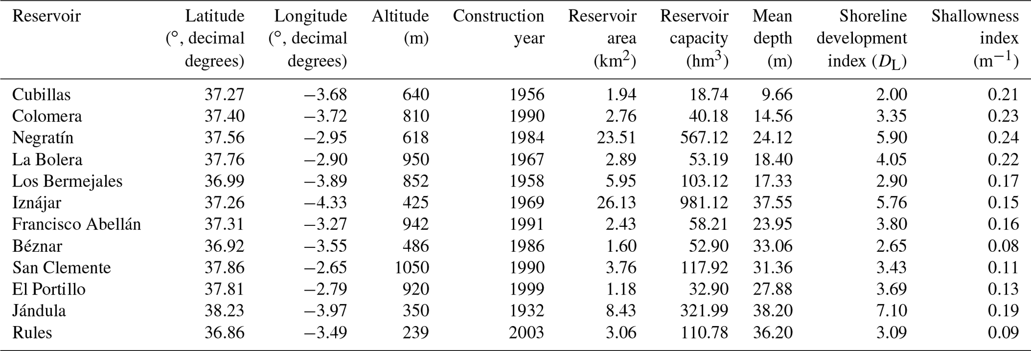
Download Print Version | Download XLSX

Table 2Sampling date; mean values of the DOC, TN, and TP concentrations; DIN : TP ratio; and chlorophyll a concentration in the water column of the studied reservoirs during the stratification and the mixing period.

Download Print Version | Download XLSX

We obtained the reservoir surface area, perimeter, and volume using the following open databases: Infraestructura de Datos Espaciales de Andalucía (IDEAndalucia; http://www.ideandalucia.es/portal/web/ideandalucia/, last access: 4 February 2018).) and the Ministerio para la Transición Ecológica (https://www.embalses.net/, last access: 15 September 2019).

The mean depth was calculated as follows (Eq. 1):

\begin{matrix} (1) & Mean depth (m) = \frac{Volume (m^{3})}{Surface area (m^{2})} . \end{matrix}

The shoreline development ratio (D_L) (Aronow, 1982) is a comparative index relating the shoreline length (i.e., the perimeter of the reservoir) to the circumference of a circle that has the same area. The closer this ratio is to 1, the more circular the lake. A large ratio (≫1) indicates that the shoreline is more scalloped than a low ratio. The equation is as follows (Eq. 2):

\begin{matrix} (2) & D_{L} = \frac{Length of the shoreline (m)}{2 \sqrt{π Area (m^{2})}} . \end{matrix}

The shallowness index (m⁻¹) was obtained by dividing the shoreline development index (D_L) by the mean depth (m), as in Eq. (3):

\begin{matrix} (3) & Shallowness index (m^{- 1}) = \frac{D_{L}}{Mean depth (m)} . \end{matrix}

We sampled the water column near the dam, in the open water of the reservoir. During the stratification and the mixing period, we selected the same location. First, we performed a vertical profile of the reservoir using a Sea-Bird 19plus CTD profiler, coupled to a Spherical Underwater Quantum Sensor (LI-193R), and a fluorimeter Turner^® SCUFA (model CYCLOPS-7) for continuous measurements of temperature (^∘C), dissolved oxygen (µmol L⁻¹), conductivity (µS cm⁻¹), turbidity (FTU – formazin turbidity unit), density (kg m⁻³), photosynthetic active radiation, chlorophyll a fluorescence (µg L⁻¹), specific conductance (µS cm⁻¹), and salinity (psu – practical salinity units). Then, based on the temperature and oxygen profiles, we selected six to nine depths, representative of the oxic and anoxic layers and the transition between them in the different reservoirs. We took the water samples using a UWITEC sampling bottle of 5 L with a self-closing mechanism. We collected samples for the dissolved CH₄ analysis in 125 or 250 mL airtight Winkler bottles in duplicate (250 mL) or in triplicate (125 mL). We filled up the bottles very carefully from the bottom to avoid the formation of bubbles and minimize the loss of CH₄ during field sampling. We preserved the samples with a solution of HgCl₂ (final concentration 1 mmol L⁻¹) to inhibit biological activity and sealed the bottles with Apiezon^® grease to prevent gas exchanges. We also took samples from each depth from the chemical and biological analysis explained below. We also measured barometric pressure using a multi-parameter probe (Hanna HI 9828) for the gas saturation calculations. We calculated the saturation values (%) for dissolved oxygen as the ratio of the dissolved gas measured and the gas concentration expected in equilibrium. We calculated the gas concentration in equilibrium, taking into account the differences in temperature, salinity, and barometric pressure (Mortimer, 1956).

2.2 Dissolved CH₄ in the water column

We stored the Winkler bottles in the dark at room temperature until analysis in the laboratory. We measured dissolved CH₄ using headspace equilibration in a 50 mL airtight glass syringe (Agilent P/N 5190–1547) (Sierra et al., 2017). We obtained two replicates for each 150 mL Winkler bottle and three replicates for each 250 mL Winkler bottle. We took a quantity of 25 g of water (±0.01 g) using the airtight syringe and added a quantity of 25 mL of a standard gas mixture that had a methane concentration similar to atmospheric values (1.8 ppmv) to complete the volume of the syringe. The syringes were shaken for 5 min (Vibromatic, Selecta) to ensure mixing, and we waited 5 min to reach complete equilibrium. Then, the gas in the syringe was injected manually into the gas chromatograph (GC; Bruker^® GC-450) equipped with a hydrogen flame ionization detector (FID). We calibrated the detectors daily using three standard gas mixtures with CH₄ mixing ratios of 1952, 10 064, and 103 829 ppbv, made and certified by Air Liquide (France). We calculated the gas concentration in the water samples from the concentration measured in the headspace using the Bunsen functions for CH₄ (Yamamoto et al., 1976; Wiesenburg and Guinasso, 1979). The precision in the quantification of the gas mixture of CH₄ used in the headspace equilibrium (1.8 ppmv) expressed as the coefficient of variation was 3.7 % (n=123). The precision of the measurement of the dissolved CH₄ concentration, which included the analytical processing of the samples and the equilibration step, was 3.6 % for four to six replicates of each sample. We calculated the saturation values (%) as the ratio of the concentration of the dissolved gas measured to the gas concentration expected in equilibrium considering the temperature, salinity, and barometric pressure of each reservoir. We used the atmospheric gas concentrations provided by the Global Greenhouse Gas Reference Network website (https://www.esrl.noaa.gov/gmd/ccgg/index.html, last access: 20 September 2019), which is part of the National Oceanic and Atmospheric Administration (NOAA) Earth System Research Laboratory in Boulder, Colorado. We calculated the 2016 global mean atmospheric concentrations for CH₄ (Dlugokencky, 2019) from the 2016 global monthly mean. The differences among these values and the local atmospheric concentrations are assumed to be small compared with the high dissolved concentrations obtained in the studied reservoirs.

2.3 Chemical analysis in the water column

From the discrete sampling, we selected thee or four representative depths of the epilimnion, metalimnion (oxycline), and hypolimnion and bottom layers for nutrient analysis during the stratification period. We also selected three or four equivalent depths during the mixing period. In total, we analyzed 77 samples: 41 samples from the stratification period and 36 samples from the mixing period. We determined total nutrients using unfiltered water, while we filtered the samples through pre-combusted 0.7 µm pore-size Whatman GF/F glass-fiber filters for the dissolved nutrients. We acidified the samples for dissolved organic carbon (DOC), total dissolved nitrogen (TDN), and total nitrogen (TN) with phosphoric acid (final pH <2). We measured DOC, TN, and TDN by high-temperature catalytic oxidation using a Shimadzu total organic carbon (TOC) analyzer (Model TOC-VCSH) coupled to a nitrogen analyzer (TNM-1). We calibrated the instrument using a four-point standard curve of dried potassium hydrogen phthalate for DOC and dried potassium nitrate for TN and TDN (Álvarez-Salgado and Miller, 1998). We analyzed two replicates and three to five injections per replicate for each sample. We purged the DOC samples with phosphoric acid for 20 min to eliminate all the dissolved inorganic carbon. The precision of the DOC measurements expressed as the mean coefficient of variation was 3.0 %. The mean precision for the TN and TDN was 8.2 % and 2.9 %, respectively.

We measured the ${NO}_{3}^{-}$ concentration in duplicate with the ultraviolet spectrophotometric method, using a Perkin Elmer UV Lambda 40 spectrophotometer at wavelengths of 220 nm and correcting for DOC absorbance at 275 nm (APHA, 1992). The mean coefficient of variation was 0.5 %. We measured ${NO}_{2}^{-}$ concentrations by inductively coupled plasma optical emission spectrometry (ICP-OES). Dissolved inorganic nitrogen (DIN) was calculated as the addition of the ${NO}_{3}^{-}$ and ${NO}_{2}^{-}$ concentrations. The detection limits for the ${NO}_{2}^{-}$ concentration was 1.4 µmol L⁻¹. We measured total phosphorus (TP) concentration in triplicate using the molybdenum blue method (Murphy and Riley, 1962) after digestion with a mixture of potassium persulfate and boric acid at 120 ^∘C for 30 min (APHA, 1992). The precision in the quantification of the TP concentration was 11.1 %.

2.4 Chlorophyll a, phytoplankton, and primary production in the water column

We determined the chlorophyll a concentration and the abundances of cyanobacteria and photosynthetic picoeukaryotes in all the depths sampled during the discrete samplings (n=178). We determined the chlorophyll a concentration by filtering the particulate material of 500 to 2000 mL of water through pre-combusted Whatman GF/F glass-fiber filters. Then, we extracted the pigments from the filters with 95 % methanol in the dark at 4 ^∘C for 24 h (APHA, 1992). We measured chlorophyll a (Chl a) absorption using a Perkin Elmer UV Lambda 40 spectrophotometer at the wavelength of 665 nm and for scattering correction at 750 nm. The detection limit was 0.1 µg L⁻¹.

To obtain the cumulative chlorophyll a in the whole water column (mg Chl a m⁻²), from the discrete depths, we summed the concentration of Chl a from each stratum using the trapezoidal rule (León-Palmero et al., 2019), as indicated in Eq. (4):

\begin{matrix} (4) & Cumulative Chl a = \sum_{k = 1}^{n} X_{i k} \cdot (Z_{k + 1} - \frac{Z_{k - 1}}{2}), \end{matrix}

where Z stands for the depth considered, and n is the number of depths sampled. Z_k stands for the n sampled depth; X_ij is the Chl a concentration (µg L⁻¹) at the depth Z_k.

We determined in triplicate the abundances of cyanobacteria and photosynthetic picoeukaryotes using flow cytometry using unfiltered water. We collected and fixed the samples with a mixture of 1 % paraformaldehyde and 0.05 % glutaraldehyde for 30 min in the dark at 4 ^∘C. Then, we froze the samples in liquid nitrogen and stored them at −80 ^∘C until analysis. We analyzed the samples in the FACSCalibur flow cytometer equipped with the BD CellQuest Pro software for data analysis. We used yellow–green 0.92 µm latex beads (Polysciences) as an internal standard to control the cytometer performance every day. We used different signals for groups determination: the side scatter (SSC), chlorophyll a (red fluorescence – FL3), phycoerythrin (orange fluorescence – FL2), and phycocyanin (blue fluorescence – FL4), following the protocols and indications for data analysis of previous works (Cellamare et al., 2010; Collier, 2000; Corzo et al., 1999; Gasol and Giorgio, 2000; Liu et al., 2014). In Fig. S13 in the Supplement, we show a cytogram of the populations of cyanobacteria and photosynthetic picoeukaryotes. The mean coefficient of variation for the abundances of cyanobacteria and photosynthetic picoeukaryotes was 8.8 % and 11.4 %, respectively.

We estimated gross primary production (GPP), net ecosystem production (NEP), and ecosystem respiration (R) by measuring temporal changes in dissolved oxygen concentration and temperature using a miniDOT (PME) submersible waterlogger during the stratification period. We recorded measurements every 10 min for 24–48 h during the same sampling days. Briefly, the equation for estimating free-water metabolism from measurements of dissolved oxygen was established by Odum (1956) (Eq. 5):

\begin{matrix} (5) & Δ O_{2} / Δ t = GPP - R - F - A, \end{matrix}

where ΔO₂∕Δt is the change in dissolved oxygen concentration through time, F is the exchange of O₂ with the atmosphere, and A is a term that combines all other processes that may cause changes in the dissolved oxygen concentration as horizontal or vertical advection, and it is often assumed to be negligible. The calculations were performed as in Staehr et al. (2010). The physical gas flux was modeled as follows (Eq. 6):

\begin{matrix} (6) & F (g O_{2} m^{- 2} h^{- 1}) = k (O_{2 meas} - O_{2 sat}), \end{matrix}

where F is the physical gas flux, and k (m h⁻¹) is the piston velocity estimated following the equation of Jähne et al. (1987) and the indications of Staehr et al. (2010). O_2 meas is the actual oxygen concentration (mg mL⁻¹), and O_2 sat is the oxygen concentration in water in equilibrium with the atmosphere at ambient temperature and salinity.

We calculated the hourly net ecosystem production (NEP_hr) and the daytime net ecosystem production (NEP_daytime) following Eqs. (7) (Cole et al., 2000) and (8):

\begin{matrix} (7) & {NEP}_{hr} (g O_{2} m^{- 3} h^{- 1}) = Δ O_{2} (g m^{- 3} h^{- 1}) - F / Z_{mix}, \\ (8) & \begin{aligned} {NEP}_{daytime} (g O_{2} m^{- 3} daylight {period}^{- 1}) \\ = mean {NEP}_{hr} during daylight (g O_{2} m^{- 3} h^{- 1}) \\ \times Light hours (h) . \end{aligned} \end{matrix}

NEP_hr is directly derived from the changes in dissolved oxygen (ΔO₂), after accounting for physical gas flux with the atmosphere (F). Z_mix is the depth of the mixed layer (m), which was inferred from the temperature profile as the upper mixed zone where the temperature remains constant. NEP_daytime is the portion of NEP between sunrise and sunset, when the photosynthesis takes place. We obtained the exact light hours from an online solar calculator (https://es.calcuworld.com/calendarios/calcular-salida-y-puesta-del-sol/, last access: 24 May 2018). We established the start and the end time for photosynthesis as 30 min before sunrise and 30 min after dawn (Schlesinger and Bernhardt, 2013). We obtained hourly R (R_hr), R during the daytime (R_daytime), and R throughout the whole day (R_day), following Eqs. (9), (10), and (11), respectively:

\begin{matrix} (9) & \begin{aligned} R_{hr} (g O_{2} m^{- 3} h^{- 1}) \\ = mean {NEP}_{hr} during darkness (g O_{2} m^{- 3} h^{- 1}), \end{aligned} \\ (10) & \begin{aligned} R_{daytime} (g O_{2} m^{- 3} daylight {period}^{- 1}) \\ = R_{hr} (g O_{2} m^{- 3} h^{- 1}) \times Light hours (h), \end{aligned} \\ (11) & R_{day} (g O_{2} m^{- 3} d^{- 1}) = R_{hr} (g O_{2} m^{- 3} h^{- 1}) \times 24 (h) . \end{matrix}

We calculated the respiration rate during the night (the period between 60 min after dawn and 60 min before sunrise) (Staehr et al., 2010), and we assumed that the respiration rate overnight was similar to the respiration rate throughout the day. Finally, we obtained the GPP and NEP for the day (Eqs. 12 and 13):

\begin{matrix} (12) & GPP (g O_{2} m^{- 3} d^{- 1}) = {NEP}_{daytime} + R_{daytime}, \\ (13) & NEP (g O_{2} m^{- 3} d^{- 1}) = GPP - R_{day} . \end{matrix}

2.5 DNA analysis

We selected three or four representative depths for determining the abundance of the functional genes of the epilimnion, metalimnion (oxycline), and hypolimnion and bottom layers during the stratification period. We also selected three or four equivalent depths during the mixing period. In total, we analyzed 41 samples from the stratification period and 36 samples for the mixing period. We pre-filtered the water through 3.0 µm pore-size filters and extracted DNA following the procedure developed by Boström et al. (2004) for environmental samples. During the DNA extraction protocol, we combined a cell recovery step by centrifugation of 12–20 mL of the pre-filtered water, a cell lysis step with enzyme treatment (lysozyme and proteinase K), and, finally, the DNA recovery step with a co-precipitant (yeast tRNA) to improve the precipitation of low-concentration DNA. DNA was quantified using a DNA quantitation kit (Sigma-Aldrich) based on the fluorescent dye bisbenzimide (Hoechst 33258). Extracted DNA served as the template for PCR and quantitative PCR (qPCR) analysis to test the presence and abundance of the mcrA gene and the phnJ gene. For PCR analysis, we used the recombinant Taq DNA Polymerase (Thermo Fisher Scientific) using the Mastercycler X50 thermal cycler (Eppendorf). We ran the qPCR plates using SYBR Green as the reporter dye (PowerUp™ SYBR™ Green Master Mix, Thermo Fisher Scientific) in the Applied Biosystems 7500 Real-Time PCR System and the 7500 Software. In both cases, PCR and qPCR, we designed the standard reaction mix recipes and the thermocycling conditions using the provider specifications and primer requirements. We chose specific primers from studies performed in natural samples of freshwater. We used pure cultures as positive controls (more details below).

We targeted the alpha subunit of methyl-coenzyme reductase (mcrA) as a genetic marker to determine the existence and abundance of methanogenic Archaea in our samples. This gene appears to be an excellent marker, since all known methanogens have the methyl-coenzyme M reductase, which is the enzyme responsible for the conversion of a methyl group to CH₄ (Grabarse et al., 2001). We used specific primers from West et al. (2012), adapting their procedure. The forward primer was mcrAqF (5^′-AYGGTATGGARCAGTACGA-3^′), the reverse primer was mcrAqF (5^′-TGVAGRTCGTABCCGWAGAA-3^′), and the annealing temperature was 54 ^∘C. The expected size of the PCR product was ∼200 bp (bp – base pair). We used a culture of Methanosarcina acetivorans (ATCC 35395) as a positive control. We tested all the samples (n=77). We also tested the presence of the phnJ gene, which encodes a subunit of the C–P lyase complex (Seweryn et al., 2015; White and Metcalf, 2007). This enzyme cleaves C–P bonds in phosphonate compounds, releasing methane, and changes in response to the phosphate availability (Yao et al., 2016a). We ran the amplification with a pair of primers previously used by Fox et al. (2014) and Yao et al. (2016a). The forward primer was PhnJoc1 (5^′-AARGTRATMGAYCARGG-3'), and the reverse was PhnJoc2 (5^′-CATYTTYGGATTRTCRAA-3^′), adapting the PCR procedure from Yao et al. (2016a). The annealing temperature was 52.5 ^∘C, and the positive controls were run using a pure culture of Rhodopseudomonas palustris (ATCC 33872). The expected size of the PCR product was ∼400 bp. We checked the result of the amplification by running 1.5 % (w∕v) agarose gel electrophoresis. If we did not detect amplification in the PCR or qPCR samples, we changed the standard procedure by increasing the DNA amount and the primers' concentration to corroborate the negative results. We tested all the samples (n=77).

2.6 Statistical tests

We conducted all the statistical analysis in R (R Core Team, 2014), using the packages “car” (Fox and Weisberg, 2011), “nortest” (Gross and Ligges, 2015), and “mgcv” (Wood, 2011). We performed the Shapiro–Wilk test of normality analysis and Levene's test for homogeneity of variance across groups. We performed a one-way analysis-of-variance test (ANOVA) when the data were normally distributed. In case the data did not meet the assumptions of normality, we used the paired Kruskal–Wallis rank-sum (K–W) or Wilcoxon (V) tests. We analyzed the potential sources of dissolved CH₄ using simple regression analysis and generalized additive models (GAMs) (Wood, 2006). A GAM is a generalized model with a linear predictor involving a sum of smooth functions of covariates (Hastie and Tibshirani, 1986, 1990). The model structure is shown in Eq. (4):

\begin{matrix} (4) & y_{i} = f_{1} (x_{1 i}) + f_{2} (x_{2 i}) + \dots + f_{n} (x_{n i}) + \in_{i}, \end{matrix}

where f_j is the smooth functions, and ∈_i is independent identically distributed N (0,σ²) random variables. We fit smoothing functions by penalized cubic regression splines. The cross-validation method (generalized cross-validation – GCV – criterion) estimates the smoothness of the functions. We fitted the models to minimize the Akaike information criterion (AIC) and the GCV values. We calculated the percentage of variance explained by the model (adjusted R²) and the quality of the fit (deviance explained). We also fixed the effect of each predictor to assess the contribution of the other predictor on the total deviance explained. Then, the sum of the deviance explained by two predictors can be different from the deviance explained by the model due to interactive effects.

3 Results and discussion

3.1 Profile description

We found pronounced differences in the concentration of dissolved CH₄ of the studied reservoirs among depths and seasonal periods (Figs. 2–4 and S1–9). The concentration of dissolved CH₄ ranged up to 4 orders of magnitude, from 0.06 to 213.64 µmol L⁻¹, during the summer stratification (n=96), and it was less variable during the winter mixing (n=84), ranging only from 0.02 to 0.69 µmol L⁻¹. All depths were consistently supersaturated in CH₄, during both the stratification and mixing period (Table S1 in the Supplement). The dissolved CH₄ concentration and the percentage of saturation values were significantly higher during the stratification period than during the mixing period (V=78, p value <0.001, and V=78, p value <0.001, respectively). These differences in the concentration of dissolved CH₄ are coherent with the differences found in the CH₄ emissions from these reservoirs in the stratification and mixing periods (León-Palmero et al., 2020). The wide range in CH₄ concentrations found in this study covers values reported in temperate lakes (Donis et al., 2017; Grossart et al., 2011; Tang et al., 2014; West et al., 2016), to those found in tropical lakes and reservoirs (Murase et al., 2003; Naqvi et al., 2018; Okuku et al., 2019; Roland et al., 2017). In the surface mixing layer during the stratification period (i.e., epilimnion), we found values from 0.06 to 8.18 µmol L⁻¹ (Table S1), which is about 80 times the maximum values found in the surface waters of Lake Kivu (Africa) by Roland et al. (2017) and similar to the concentrations reported in subtropical and tropical reservoirs (Musenze et al., 2014, and references therein).

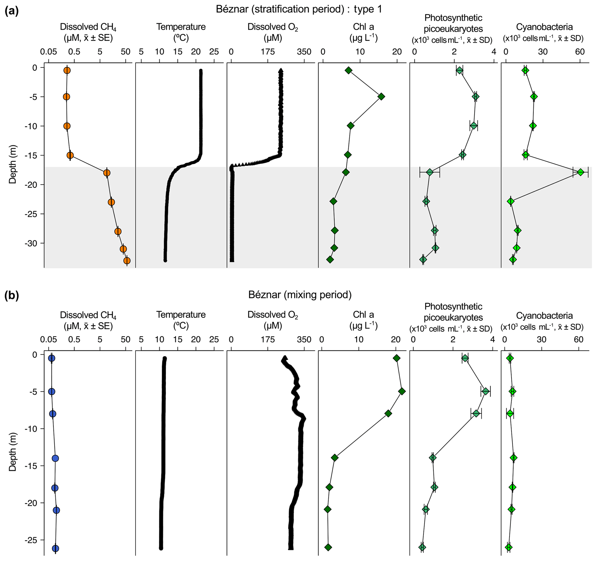
https://www.biogeosciences.net/17/3223/2020/bg-17-3223-2020-f02

Figure 2Vertical profiles of physicochemical and biological variables in Béznar reservoir. Dissolved methane concentration (CH₄, µM, mean ± standard error), temperature (^∘C), dissolved oxygen (DO) concentration (µM), chlorophyll a (Chl a) concentration (µg L⁻¹), abundance of photosynthetic picoeukaryotes (×10³ cells mL⁻¹, mean ± standard deviation), and abundance of cyanobacteria (×10³ cells mL⁻¹, mean ± standard deviation) during the stratification period (a) and the mixing period (b). The grey area represents the anoxic zone (DO <7.5 µM). Note the logarithmic scales in the x axis of the dissolved CH₄ profiles. The sampling for the stratification period was on 7 October 2016 and 23 February 2017 for the mixing period.

Download

https://www.biogeosciences.net/17/3223/2020/bg-17-3223-2020-f03

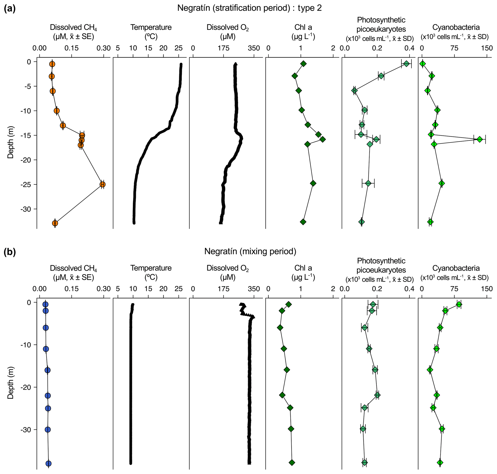
Figure 3Vertical profiles of physicochemical and biological variables in Negratín reservoir. Dissolved methane concentration (CH₄, µM, mean ± standard error), temperature (^∘C), dissolved oxygen (DO) concentration (µM), chlorophyll a (Chl a) concentration (µg L⁻¹), abundance of photosynthetic picoeukaryotes (×10³ cells mL⁻¹, mean ± standard deviation), and abundance of cyanobacteria (×10³ cells mL⁻¹, mean ± standard deviation) during the stratification period (a) and the mixing period (b). The sampling for the stratification period was on 27 July 2016 and 16 February 2017 for the mixing period.

Download

The dissolved CH₄ profiles showed considerable differences among depths during the summer stratification (Figs. 2a–4a and S1a–9a) but were very homogeneous during the winter mixing in all the reservoirs (Figs. 2b–4b and S1b–9b) (Table S1). Based on the differences found during the stratification period in the dissolved CH₄ profiles, we sorted the reservoirs into three types. The first type of CH₄ profile included six reservoirs that were characterized by an increase in the dissolved CH₄ from the oxycline to the anoxic bottom, just above the sediments, where CH₄ concentration reached its maximum. In these reservoirs, the oxycline may be spatially coupled to the thermocline or not. When the oxycline and the thermocline were spatially coupled, the dissolved CH₄ concentration increased exponentially from the thermocline along the anoxic hypolimnion to the sediments. The reservoirs Béznar, San Clemente, and Iznájar showed this type of profile (Figs. 2a, S1a, and S2a). The existence of a sizeable almost-anoxic hypolimnion led to a massive accumulation of CH₄ in this layer. The differences in the CH₄ concentration between the surface and bottom waters were up to 3 orders of magnitude, as we found in Béznar (from the 0.25 to 56.17 µmol L⁻¹; Fig. 2a), San Clemente (from the 0.23 to 45.15 µmol L⁻¹; Fig. 1a), and Iznájar (from the 0.82 to 213.64 µmol L⁻¹; Fig. S2a). When the oxycline and the thermocline were not spatially coupled, the dissolved CH₄ concentration increased just above the sediments, where the anoxic–oxic interface was near to the bottom. The reservoirs Cubillas, La Bolera, and Francisco Abellán showed this profile type (Figs. S3a, S4a, and S5a). This accumulation of CH₄ in the hypolimnion and above sediments might be related to the high rates of methanogenesis in the sediments and its subsequent diffusion to the water column. Dissolved CH₄ concentration declines at the oxycline level, where the highest rates of CH₄ oxidation usually occur (Oswald et al., 2015, 2016). The CH₄ profiles in this group were similar to the ones found in tropical eutrophic and temperate reservoirs (Naqvi et al., 2018; West et al., 2016). The second profile type presents a small peak of metalimnetic CH₄, concomitant with peaks of dissolved oxygen, chlorophyll a, photosynthetic picoeukaryotes, and cyanobacteria (Fig. 3a). In the Negratín reservoir, we found the maximum concentration of CH₄ in the oxic hypolimnion. Unlike several previous works in lakes (Blees et al., 2015; Grossart et al., 2011; Khatun et al., 2019; Murase et al., 2003), we did not find a metalimnetic CH₄ maximum. Khatun et al. (2019) described the existence of a metalimnetic CH₄ maximum in 10 out of 14 lakes. The metalimnetic CH₄ maximum may represent a physically driven CH₄ accumulation due to solubility differences with the temperature at the thermocline, the epilimnetic CH₄ losses by emission, and the lateral inputs from the littoral zone (Donis et al., 2017; Encinas Fernández et al., 2016; Hofmann et al., 2010). The metalimnetic CH₄ maximum can also be determined by biological factors, including the light inhibition of the methane oxidation (Murase and Sugimoto, 2005; Tang et al., 2014) or the distinctive methane production by phytoplankton due to availability of nutrients, light, or precursors at this layer (Khatun et al., 2019). The third profile type included five reservoirs, in which the dissolved CH₄ profile presented a CH₄ accumulation more significant in the epilimnion than in the hypolimnion. The reservoirs Jándula, Bermejales, Rules, El Portillo, and Colomera showed this profile type (Figs. 4a and S6a–9a). These reservoirs had a mean CH₄ concentration in the water column significantly lower than the reservoirs from the first type. Similar profiles have been reported in temperate (Tang et al., 2014) and tropical lakes (Murase et al., 2003).

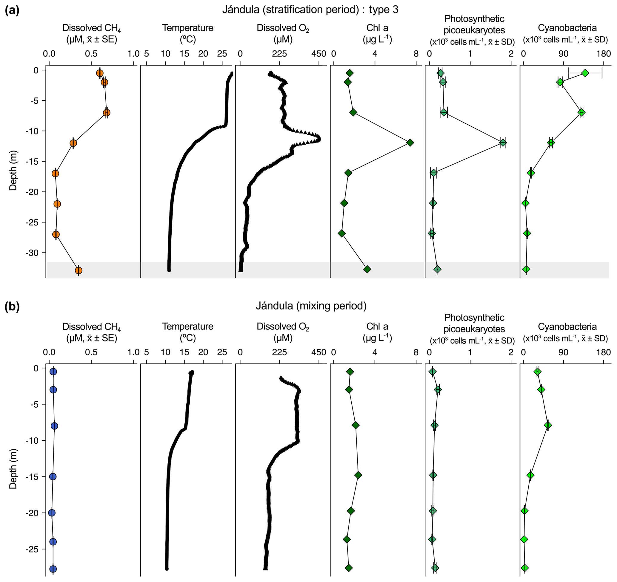
https://www.biogeosciences.net/17/3223/2020/bg-17-3223-2020-f04

Figure 4Vertical profiles of physicochemical and biological variables in Jándula reservoir. Dissolved methane concentration (CH₄, µM, mean ± standard error), temperature (^∘C), dissolved oxygen (DO) concentration (µM), chlorophyll a (Chl a) concentration (µg L⁻¹), abundance of photosynthetic picoeukaryotes (×10³ cells mL⁻¹, mean ± standard deviation), and abundance of cyanobacteria (×10³ cells mL⁻¹, mean ± standard deviation) during the stratification period (a) and the mixing period (b). The grey area represents the anoxic zone (DO <7.5 µM). The sampling for the stratification period was on 24 July and 5 April 2017 for the mixing period.

Download

3.2 CH₄ sources in the water column

We found two well-differentiated groups of CH₄ data sorted by the dissolved oxygen (DO) concentration (Fig. S10), as in previous studies (Tang et al., 2014). The first dataset included the samples with a DO lower than 7.5 µmol L⁻¹ (n=18, hereafter anoxic samples). These samples belong to the hypolimnion of the studied reservoirs during the stratification period. The second dataset included the samples with DO higher than 7.5 µmol L⁻¹ (n=160, hereafter oxic samples). All the samples from the mixing period (n=82) and most of the samples from the stratification period (n=78) belong to this second dataset. We found significant differences (W=2632, p value <0.001) between the concentration of CH₄ in the anoxic samples (median = 15.79, min = 0.35, max = 213.64 µmol L⁻¹) and in the oxic samples (median = 0.15, min = 0.02, max = 8.17 µmol L⁻¹). Since these two groups of samples are different, we determined their sources and drivers separately (Table S2).

3.2.1 CH₄ sources in anoxic waters

Archaeal methanogens are obligate anaerobes that decompose the organic matter and produce CH₄ in anoxic environments, as freshwater sediments. We analyzed the presence of the methanogenic Archaea in the anoxic samples of the water column by targeting the gene mcrA. From the 77 samples selected for genetic analysis, 12 of them were anoxic. We did not detect the amplification of the mcrA gene in the PCR or the qPCR analysis in these 12 samples. Therefore, we assumed that the methanogenic Archaea were not present, as free-living microorganisms, in the water column of the anoxic samples. However, they may still be present in micro-anoxic zones in the water column (i.e., in the guts of zooplankton or within exopolymeric particles). Methanogenesis is a microbial process particularly sensitive to temperature (Marotta et al., 2014; Sepulveda-Jauregui et al., 2018; Yvon-Durocher et al., 2014). However, we did not find a significant relationship between the water temperature and the dissolved CH₄ concentration in the anoxic samples (n=17, p value =0.66). The lack of a detection of the mcrA gene in the hypolimnetic waters and the absence of a relationship between the dissolved CH₄ and water temperature suggest that CH₄ production is not happening in the water column of the studied reservoirs. We think that most methanogenic archaea must be present in the sediments, where they produce CH₄ that diffuses up to the water column, producing vast accumulations of CH₄ in the hypolimnion.

Methanogenesis in the sediments may be affected by organic matter quantity and quality (West et al., 2012). Organic matter quantity is measured as the dissolved organic carbon concentration, whereas the organic matter quality usually is related to their phytoplanktonic versus terrestrial origin. In the studied reservoirs, the dissolved organic carbon concentration did not show a significant relationship with the dissolved CH₄ concentration (n=12, p value =0.10; Table S2). We examined the importance of the autochthonous organic matter produced by primary producers using the total cumulative Chl a (mg m⁻²). The cumulative Chl a is considered to be a surrogate for the vertical export of the phytoplankton biomass in the whole water column. We found that the CH₄ concentrations in anoxic samples were correlated to the cumulative Chl a following a power function (CH₄ = $3.0 \times 10^{- 4}$ cumulative Chl a^2.28, n=17, adjusted R²=0.40, p value <0.01; Table S2) (Fig. 5). The autochthonous organic matter appeared to be a better predictor for the concentration of CH₄ in anoxic waters than the dissolved organic matter concentration. In the studied reservoirs, the dissolved organic carbon concentration was significantly related to the age of the reservoirs and the forestry coverage in their watersheds (León-Palmero et al., 2019). Therefore, in terms of quality, the total pool of dissolved organic carbon may be more representative of the carbon fraction that is allochthonous, recalcitrant, and more resistant to microbial degradation. In contrast, the autochthonous organic matter may represent a more labile and biodegradable fraction. Previous experimental studies have demonstrated that the addition of algal biomass on sediment cores increases the CH₄ production more than the addition of terrestrial organic matter (Schwarz et al., 2008; West et al., 2012, 2015). The stimulation of the methanogenesis rates appears to be related to the lipid content in phytoplankton biomass (West et al., 2015). West et al. (2016) found a significant relationship between the chlorophyll a concentration in the epilimnion and the potential methanogenesis rates from sediment incubations. In this study, we corroborate the importance of the autochthonous-derived organic matter determining the CH₄ concentrations in anoxic waters. Since we did not detect the existence of the mcrA gene in the water column, we considered that the production of methane by methanogenic Archaea occurred primarily in the sediments and was affected by the sedimentation of organic matter derived from phytoplankton.

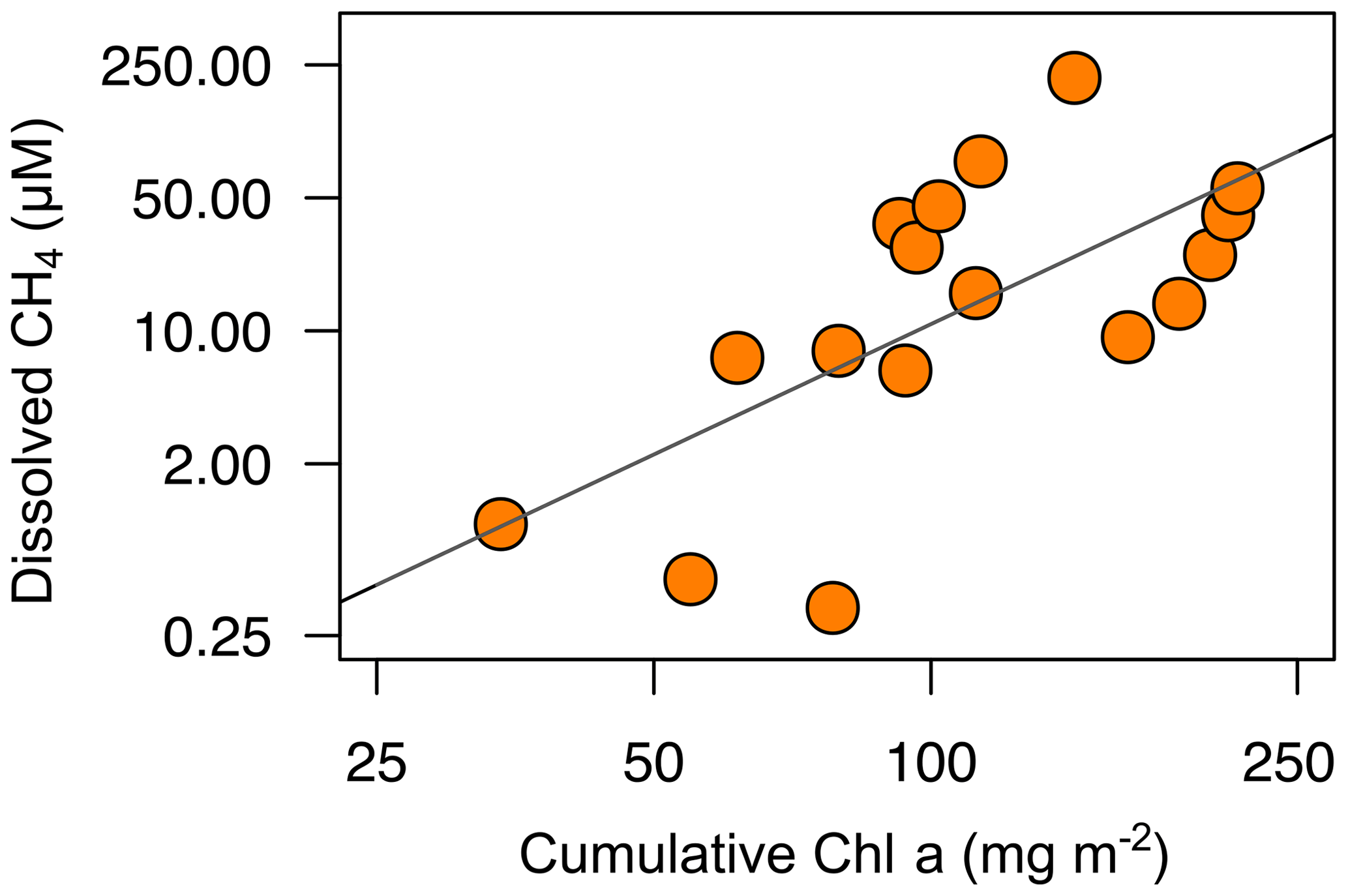
https://www.biogeosciences.net/17/3223/2020/bg-17-3223-2020-f05

Figure 5Power relationship between the depth-cumulative chlorophyll a concentration and the concentration of dissolved CH₄ in the anoxic waters during the stratification period (CH₄= $3.0 \times 10^{- 4}$ cumulative Chl a^2.28, n=17, adjusted R²=0.40). Note that both axes are at logarithmic scale. More statistical details can be found in Table S2.

Download

3.2.2 CH₄ sources in oxic waters

In this study, the concentration of dissolved CH₄ ranged from 0.02 to 8.18 µmol L⁻¹, and all the samples of the oxic waters were supersaturated, with values always above 800 % and ranging more than 2 orders of magnitude (Table S1). To determine the origin of this CH₄ supersaturation, we examined the following potential sources: (1) the vertical and lateral CH₄ transport from deep layers and littoral zones, (2) the in situ CH₄ production by methanogenic Archaea potentially tolerant to oxygen or by the methylphosphonate degradation under severe P limitation, and (3) the in situ CH₄ production by processes associated to the phytoplanktonic community.

Vertical and lateral CH₄ transport from anoxic sediments to oxic waters

Several previous works have pointed out that CH₄ supersaturation in oxic waters can be explained by the vertical transport from the bottom sediments and the lateral inputs from the littoral zones that are in contact with shallow sediments where methanogenesis occurs (Bastviken et al., 2004; Encinas Fernández et al., 2016; Michmerhuizen et al., 1996). To test the importance of the lateral and vertical transport explaining the concentration of CH₄ in the oxic waters of the studied reservoirs, we used two morphometric parameters: the mean depth (m) as a proxy for the vertical transport and the shallowness index as a proxy for the lateral transport. The dissolved CH₄ concentration was an exponential decay function of the reservoir mean depth (Fig. 6a) both during the stratification period (CH₄ = $4.0 \times 10^{- 2} e^{(50.0 / mean depth)}$ , adjusted R²=0.95) and during the mixing period (CH₄ $= 3.7 \times 10^{- 2} e^{(22.9 / mean depth)}$ , adjusted R²=0.54) (Fig. 6a). We observed that in reservoirs with a mean depth shallower than 16 m, the dissolved CH₄ concentration increased exponentially (Fig. 6a). Several studies have proposed that the vertical transport of CH₄ from bottom sediments explains the supersaturation in surface waters (Rudd and Hamilton, 1978; Michmerhuizen et al., 1996; Murase et al., 2003; Bastviken et al., 2004). However, the vertical diffusion rates of dissolved gases across the thermocline are too low in deep and thermally stratified systems, and no movements of methane upwards from the hypolimnion have been detected (Rudd and Hamilton, 1978). However, in shallow reservoirs, the hydrostatic pressure might be reduced, promoting CH₄ diffusion from the anoxic layers.

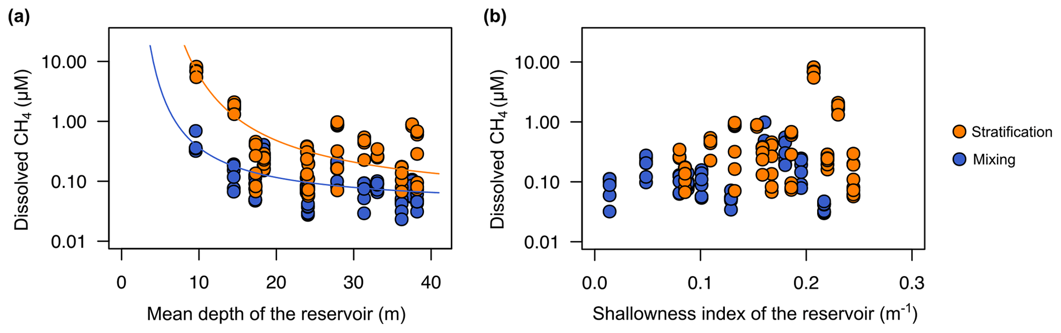
https://www.biogeosciences.net/17/3223/2020/bg-17-3223-2020-f06

Figure 6Reservoir morphometry and the dissolved CH₄ concentration in the oxic zone. (a) Exponential decay relationships of the dissolved CH₄ concentration and the mean depth (m) during the stratification period (CH₄ $= 4.0 \times 10^{- 2} e^{(50.0 / mean depth)}$ , n=78, adjusted R²=0.95) and the mixing period (CH₄ $= 3.7 \times 10^{- 2} e^{(22.9 / mean depth)}$ , n=82, adjusted R²=0.54). (b) Scatterplot of dissolved CH₄ concentration and the reservoir shallowness index during the stratification period (p value = 0.134) and the mixing period (n=0.114). More statistical details can be found in Table S2.

Download

The shallowness index increases in elongated and dendritic reservoirs, with a greater impact of the littoral zone, and decreases in near-circular reservoirs, with low shoreline length per surface. However, we did not find a significant relationship between the shallowness index and the dissolved CH₄ concentration (Fig. 6b). One explanation for the absence of this relationship could be the relatively large size of the reservoirs. Although the reservoir size covered more than 1 order of magnitude (Table 1), all reservoirs have a size larger than 1 km². Previous studies have shown that CH₄ lateral diffusion may be an important process in areas near to the littoral zone and small lakes. Hofmann et al. (2010) found higher concentrations in the shallow littoral zones than in the open waters. DelSontro et al. (2018) predicted that lateral inputs from littoral zones to pelagic waters are more critical in small and round lakes than in large and elongated lakes. Nevertheless, the differences between the observations and predictions from the model suggested that these lateral inputs may not be enough to explain CH₄ concentration in open waters, where in situ production may prevail over lateral transport (DelSontro et al., 2018).

In situ CH₄ production by methanogenic Archaea or methylphosphonate degradation

The ubiquitous CH₄ supersaturation found in oxic waters appears not to be fully explained by the vertical and lateral transport, underlining that there is an in situ production of CH₄, as proposed by Bogard et al. (2014), DelSontro et al. (2018), and Grossart et al. (2011). We studied the presence of the methanogenic Archaea in the oxic samples by targeting the gene mcrA, but we were unable to detect this gene (Fig. S11). This result indicates that methanogenic Archaea were not present, at least as free-living microorganisms, in a significant number in the water column of the oxic samples. The classical methanogens (i.e., Archaea with the mcrA gene) are obligate anaerobes without the capacity to survive and produce CH₄ under aerobic conditions (Chistoserdova et al., 1998). Previous studies by Angel et al. (2011) and Angle et al. (2017) showed that methanogens might tolerate oxygen exposure in soils, and Grossart et al. (2011) detected potential methanogenic Archaea attached to photoautotrophs in oxic lake waters. Unfortunately, we did not test their occurrence in large particles, phytoplankton, or zooplankton guts, although some authors have detected them in these microsites' particles (de Angelis and Lee, 1994; Karl and Tilbrook, 1994).

We also considered the possibility of methylphosphonate degradation as an in situ CH₄ source. This metabolic pathway appears in the bacterioplankton under chronic starvation for phosphorus (Karl et al., 2008). Several pieces of evidence have shown that marine bacterioplankton can degrade the MPn's and produce CH₄ through the C–P lyase activity in typically phosphorus-starved environments, like the ocean gyres (Beversdorf et al., 2010; Carini et al., 2014; Repeta et al., 2016; Teikari et al., 2018; del Valle and Karl, 2014). Freshwater bacteria can also degrade the MPn's and produce CH₄, as has been demonstrated in Lake Matano (Yao et al., 2016a, b). Lake Matano is an ultra-oligotrophic lake with a severe P deficiency (below 0.050 µmol P L⁻¹) due to the permanent stratification, iron content, and extremely low nutrient inputs (Crowe et al., 2008; Sabo et al., 2008). The ratio of dissolved inorganic nitrogen (DIN) to total phosphorus (TP) (µmol N : µmol P) is widely used to evaluate P limitation (Morris and Lewis, 1988). DIN : TP ratios greater than 4 are indicative of phosphorus limitation (Axler et al., 1994). In the studied reservoirs, the TP concentration ranged from 0.13 to 1.85 µmol P L⁻¹ during the stratification period and from 0.10 to 2.17 µmol P L⁻¹ during the mixing period. The mean DIN : TP ratio ranged from 12 to 675 during the stratification period and from 63 to 392 during the mixing period. The more severe the P limitation conditions are, the higher the CH₄ production by methylphosphonates degradation is. However, we did not find a significant relationship between the DIN : TP ratio and the CH₄ concentration (Fig. 7). We also analyzed the presence and abundance of the gene phnJ, which encodes the enzyme complex C–P lyase that hydrolyzes the MPn's and changes in response to phosphate availability. We did not detect the phnJ gene in the PCR or the qPCR analysis in any of the study samples (Fig. S12). These results indicate that the MPn degradation was not a quantitatively relevant source of CH₄ in the oxic waters of the studied reservoirs. Our results are in concordance with Grossart et al. (2011), who did not detect CH₄ production by adding inorganic phosphate or methylphosphonates to lake samples in laboratory experiments. Although we used different methodologies, both studies may indicate that MPn degradation is only an important source of CH₄ in ultra-oligotrophic systems, as in Lake Matano or ocean gyres.

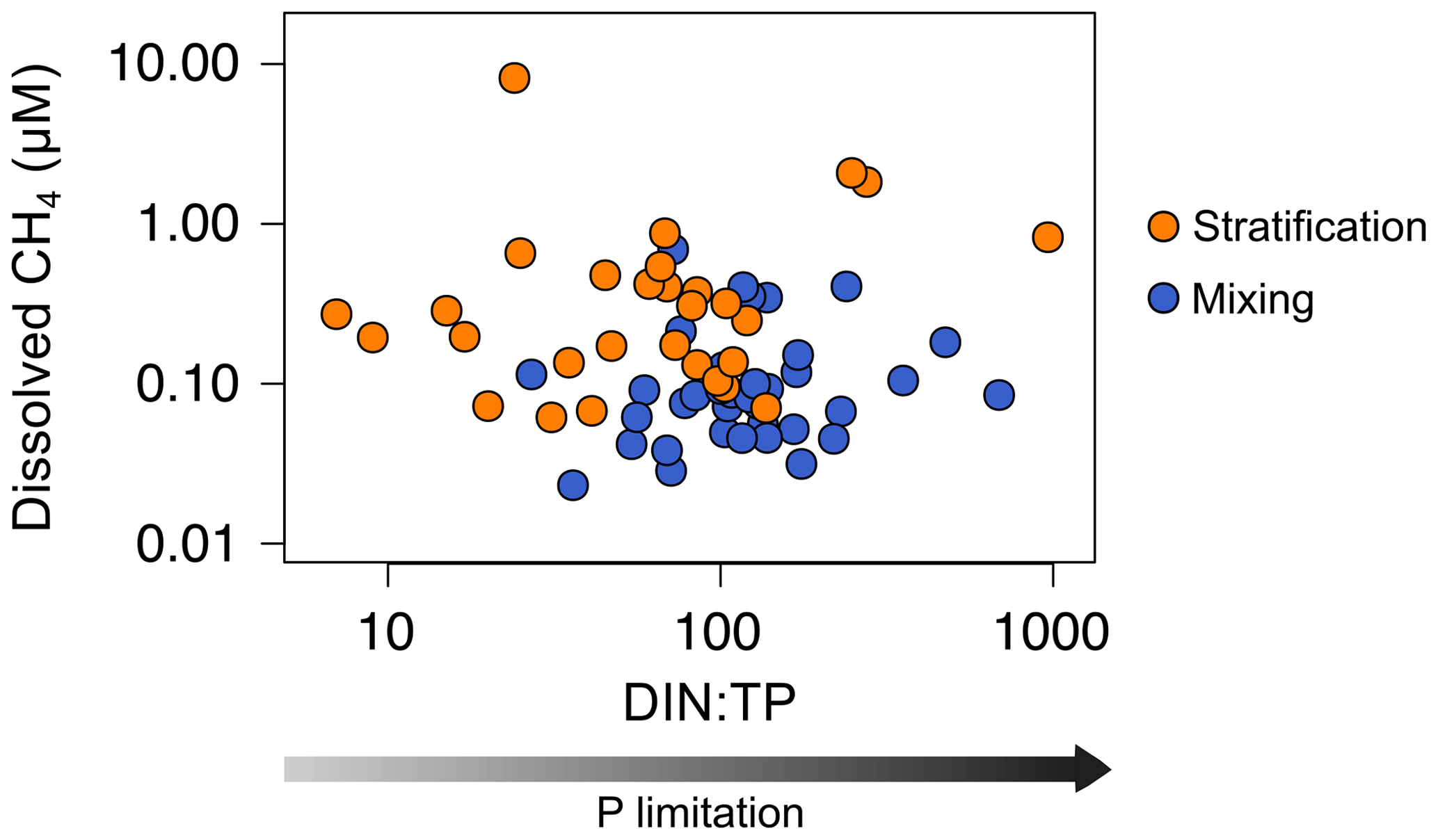
https://www.biogeosciences.net/17/3223/2020/bg-17-3223-2020-f07

Figure 7Phosphorus limitation and the dissolved CH₄ concentration in the oxic waters. Scatterplot of dissolved CH₄ concentration and the ratio between dissolved inorganic nitrogen (DIN) and the total phosphorus (TP) (µmol N : µmol P). Note the logarithmic scale in both axes.

Download

In situ CH₄ production coupled to photosynthetic organisms

In the studied reservoirs, we analyzed the relationship between photosynthetic organisms and the dissolved CH₄ concentration using the GPP (g O₂ m⁻³ d⁻¹), NEP (g O₂ m⁻³ d⁻¹), the concentration of Chl a (µg L⁻¹), and the abundance of photosynthetic picoeukaryotes (PPEs; cells mL⁻¹) and cyanobacteria (CYA; cells mL⁻¹). We determined GPP and NEP just once per reservoir during the stratification period (i.e., n=12).

The PPEs are essential components of the marine and freshwater phytoplankton, and they are eukaryotes with a size of 3.0 µm or less. In the freshwater, the PPEs include species from different phyla, like unicellular Chlorophyta (green algae) and Haptophyta. Using optical microscopy, we determined the main groups of photosynthetic picoeukaryotes in the studied reservoirs. PPEs were non-colonial green algae from the order Chlorococcales (class Chlorophyceae, phylum Chlorophyta) and the genus Chrysochromulina spp. (class Coccolithophyceae, phylum Haptophyta). The cyanobacteria detected were mainly phycoerythrin-rich picocyanobacteria, although we also detected phycocyanin-rich picocyanobacteria in one reservoir (Béznar). We show the vertical profiles of the Chl a concentration and the abundance of PPEs and CYA profiles of each reservoir in Figs. 2–4 and S1–S9. We also report the minimum, the quartiles, and the maximum values for the Chl a concentration and the abundance of PPEs and CYA during the stratification and the mixing periods in Table S2. The abundance of cyanobacteria ranged from 1.51×10³ to 2.04×10⁵ cells mL⁻¹ and was more than 1 order of magnitude higher than the abundance of PPEs that ranged from 32 to 7.45×10³ cells mL⁻¹.

Table 3Equations for the relationships between the phytoplanktonic variables and the dissolved CH₄ concentration in the oxic waters. n.m. means not measured.

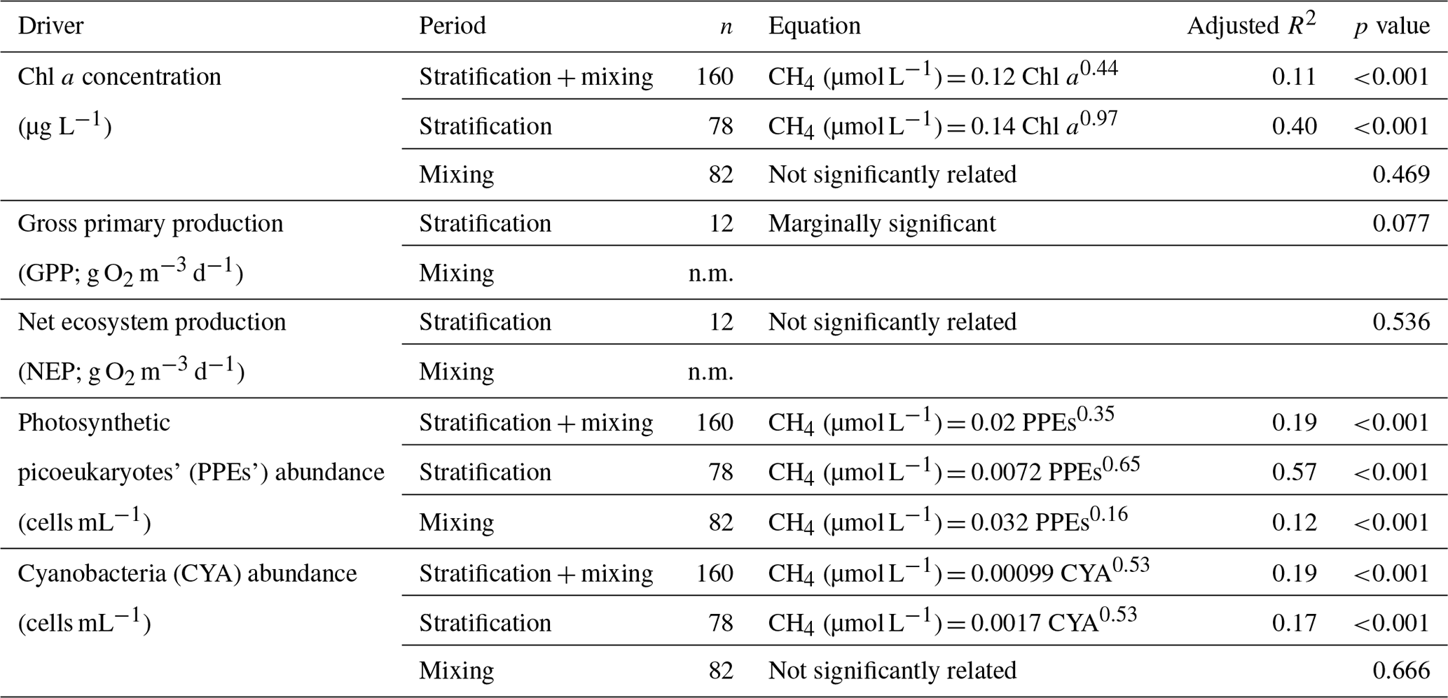
Download Print Version | Download XLSX

We found that the relationship between the gross primary production and the dissolved CH₄ concentration was only marginally significant (p value = 0.077, n=12) and not significant with the net ecosystem production (Table 3). The Chl a concentration showed a significant relationship with the GPP (p value <0.01, n=12, adjusted R²=0.55), but the abundance of cyanobacteria or the abundance of the photosynthetic picoeukaryotes did not show a significant relationship with the GPP (p value = 0.911, n=12, and p value = 0.203, n=12, respectively). We found significant power relationships between the Chl a concentration, the abundance of photosynthetic picoeukaryotes, and the abundance of cyanobacteria with the concentration of dissolved CH₄ during the stratification period (Fig. 8a, b, and c, respectively, and Table 3). During the mixing period, the only significant predictor of the dissolved CH₄ concentration was the abundance of photosynthetic picoeukaryotes (Fig. 8b). The slope of the relationship (i.e., the exponent in the power relationship) between the dissolved CH₄ and the abundance of photosynthetic picoeukaryotes was higher during the stratification than during the mixing (Table 3). By comparing the stratification slopes, the effect per cell of PPEs on CH₄ concentration was slightly higher than the impact of cyanobacteria (Table 3). These results agree with previous studies that showed a closed link between the CH₄ concentration and the photosynthetic organisms, primary production, or chlorophyll a concentration (Bogard et al., 2014; Grossart et al., 2011; Schmidt and Conrad, 1993; Tang et al., 2014). In this study, we show that the PPE abundance was a better predictor of the CH₄ concentration than the abundance of cyanobacteria. In the studied reservoirs, the PPE group included members from green algae and Haptophyta, which are regular components of the marine plankton. Therefore, these results may also be relevant for marine waters. Cyanobacteria have received more attention as potential producers of CH₄ in oxic conditions than photosynthetic picoeukaryotes (Berg et al., 2014; Bižić et al., 2020; Teikari et al., 2018). Klintzsch et al. (2019) demonstrated that widespread marine and freshwater haptophytes like Emiliania huxleyi, Phaeocystis globosa, and Chrysochromulina sp. produce CH₄ under oxic conditions. They also observed that the cell abundances were significantly related to the amount of CH₄ produced. Interestingly, Chrysochromulina was one of the genera of PPEs that we detected in the studied reservoirs. Grossart et al. (2011) also found CH₄ production in laboratory cultures of cyanobacteria and green algae.

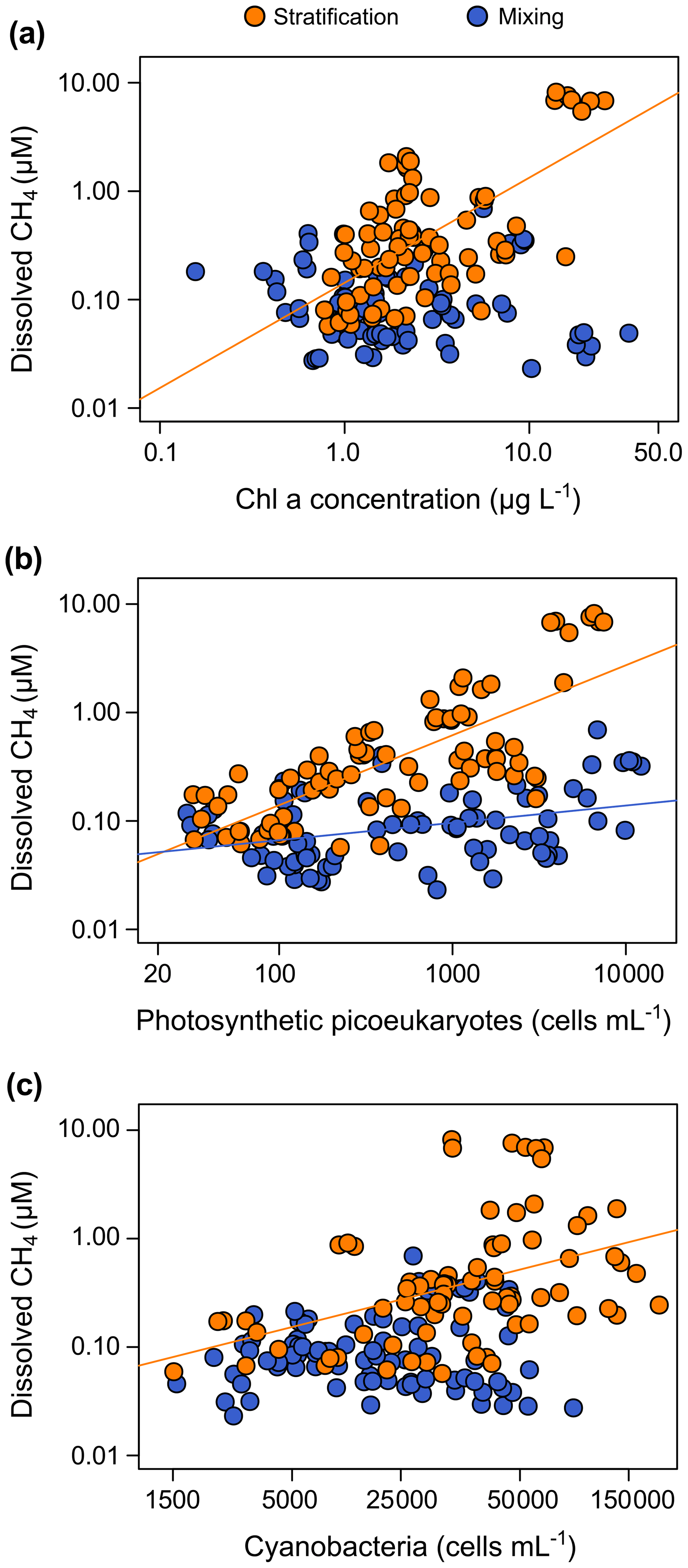
https://www.biogeosciences.net/17/3223/2020/bg-17-3223-2020-f08

Figure 8Phytoplanktonic variable coupled with the dissolved CH₄ concentration in the oxic waters. (a) The dissolved CH₄ concentration was significantly related to the chlorophyll a concentration during the stratification period (p value <0.001), but they were not related during the mixing period (p value = 0.469). The relationship during the stratification period was a power function (CH₄ = 0.14 Chl a^0.97, n=78, adjusted R²=0.40). (b) Relationships between dissolved CH₄ concentration and the abundance of photosynthetic picoeukaryotes (PPEs) during the stratification period (CH₄ = 0.0072 PPEs^0.65, n=78, adjusted R²=0.55, p value <0.001) and the mixing period (CH₄ = 0.032 PPEs^0.16, n=82, adjusted R²=0.12, p value <0.001). (c) Relationship between dissolved CH₄ concentration and the cyanobacteria abundance (CYA; cells mL⁻¹). A power function described the relationship between the dissolved CH₄ and the CYA during the stratification period (CH₄ = 0.0017 CYA^0.53, n=78, adjusted R²=0.17, p value <0.001). The relationship was not significant during the mixing period (p value = 0.666).

Download

Overall, these results indicate a clear association between the CH₄ production and the photosynthetic organisms from both Eukarya (picoeukaryotes) and Bacteria (cyanobacteria) domains. The pathways involved in the CH₄ production may be related to the central photosynthetic metabolism or the release of methylated by-products, different from methylphosphonates during the photosynthesis. Previous studies demonstrated the CH₄ production in laboratory cultures using ¹³C-labeled bicarbonate in haptophytes (Klintzsch et al., 2019; Lenhart et al., 2016); in marine, freshwater, and terrestrial cyanobacteria (Bižić et al., 2020); and in major groups of phytoplankton (Hartmann et al., 2020). In these studies, the photosynthetic organisms uptake bicarbonate in the reductive pentose phosphate cycle (Calvin–Benson cycle) (Berg, 2011; Burns and Beardall, 1987). Therefore, CH₄ production may be a common pathway in the central metabolism of photosynthesis of all the cyanobacteria and algae in freshwater and marine environments.

On the other hand, the production of CH₄ can also be related to the production of methylated compounds during photosynthesis. Lenhart et al. (2016) and Klintzsch et al. (2019) also detected the CH₄ production in cultures from the sulfur-bound methyl group of the methionine and methyl thioethers. Common substances like methionine can act as a methyl-group donor during the CH₄ production in plants and fungi (Lenhart et al., 2012, 2015). Besides, algae use part of the methionine for the synthesis of dimethylsulfoniopropionate (DMSP), an abundant osmolyte, the precursor of dimethyl sulfide (DMS), and dimethyl sulfoxide (DMSO). These methylated substances produce methane during their degradation (Damm et al., 2008, 2010, 2015; Zindler et al., 2013). Bižić-Ionescu et al. (2018) also suggested that CH₄ could be produced from methylated amines under oxic conditions. These substances, together with other organosulfur compounds, can also produce CH₄ abiotically (Althoff et al., 2014; Bižić-Ionescu et al., 2018). The production of DMSP, DMS, and other methylated substances like isoprene has been extensively studied in marine phytoplankton, showing that taxa as photosynthetic picoeukaryotes and the cyanobacteria are relevant sources (Shaw et al., 2003; Yoch, 2002). Recent studies have also reported that freshwater algae and cyanobacteria also produced DMS and isoprene (Steinke et al., 2018). Further studies are needed to quantify the potential role of all these methylated by-products as potential CH₄ sources quantitatively relevant in freshwater.

3.2.3 Modeling the CH₄ production in oxic waters

The explanation of the CH₄ supersaturation in oxic waters in relatively large systems relies on the interaction of several processes as the transport from anoxic environments and the biological activity (DelSontro et al., 2018). In this study, we found that vertical transport (mean depth as surrogate), water temperature, and the abundance of photosynthetic picoeukaryotes and cyanobacteria had a significant effect on the dissolved CH₄ concentration. We combined these explanatory variables with significant effects using GAMs. The GAM for the stratification period (n=78) had a fit deviance of 82.7 % and an explained variance (adjusted R²) of 81.4 % (Table S3). The explanatory variables, in decreasing order, were as follows: the photosynthetic picoeukaryotes' abundance (log₁₀ PPEs), the reservoir mean depth, the cyanobacteria abundance (log₁₀ CYA), and the water temperature (Fig. 9a). The function obtained was as follows: log₁₀ CH₄ $= - 4.05 + 0.34$ log₁₀ PPEs $+ e^{(6.7 / mean depth)} + 0.17$ log₁₀ CYA + 0.027 Temperature. The abundance of PPEs was the variable explaining most of the variance of dissolved CH₄ concentration (log₁₀ CH₄) during the stratification period, with an effect higher than the cyanobacteria abundance. Figure 9b–e shows the partial responses of each explanatory variable.

https://www.biogeosciences.net/17/3223/2020/bg-17-3223-2020-f09

Figure 9Results of the generalized additive model (GAM) fitted for the concentration of dissolved CH₄ in the oxic waters during the stratification period. (a) Bar plot showing the significance of the smooth terms from the fitted GAM (F values). (b–e) Partial response plots from the fitted GAM, showing the additive effects of the covariates on the dissolved CH₄ concentration: the photosynthetic picoeukaryotes' abundance (log₁₀ PPEs) (b), the mean depth (c), the cyanobacteria abundance (log₁₀ CYA) (d), and water temperature (e). In partial response plots, the lines are the smoothing functions, and the shaded areas represent 95 % pointwise confidence intervals. Rugs on x axis indicate the distribution of the data. More details are provided in Table S3.

Download

The GAM for the mixing period (n=82) only included two explanatory variables: the reservoir mean depth and the abundance of the photosynthetic picoeukaryotes. The reservoir mean depth was the variable explaining most of the variance of the dissolved CH₄ concentration (log₁₀ CH₄) during the mixing period, closely followed by the abundance of PPEs (Fig. 10a). We observed that the function of the effect of the mean depth on the CH₄ concentration changed between the two periods (Figs. 9c and 10b). The function was more linear during the mixing period than during the stratification period, likely because the mixed water column enabled the more uniform distribution of the CH₄ produced in the sediment, while the thermocline acted as a barrier to the diffusion during the stratification period. The model function for the mixing period was log₁₀ CH₄ $= - 2.07 + 1.5 e^{(- 0.04 mean depth)} + 0.18$ log₁₀ PPEs, with a fit deviance of 53.9 % and an explained variance (adjusted R²) of 52.1 % (Table S3). In Fig. 10b and c, we show the partial response plots for these two variables. The results show that the abundance of photosynthetic picoeukaryotes can be key for explaining the dissolved CH₄ concentration in oxic waters, even though they have received less attention than cyanobacteria in previous studies (Berg et al., 2014; Bižić et al., 2020; Teikari et al., 2018). Finally, we have also included a simple model to explain the dissolved CH₄ concentration (log₁₀ CH₄) using the data of both periods (n=160) and including widely used variables like the water temperature (^∘C), mean depth (m), and Chl a concentration (µg L⁻¹) for future comparisons. The function of this model is $\log_{10} {CH}_{4} = - 2.02 + 0.05 Temperature + e^{(7.73 / mean depth)} - e^{(- 0.05 \log_{10} (Chl a))}$ . This GAM had a fit deviance of 69.3 % and an explained variance (adjusted R²) of 68 % (Table S3).

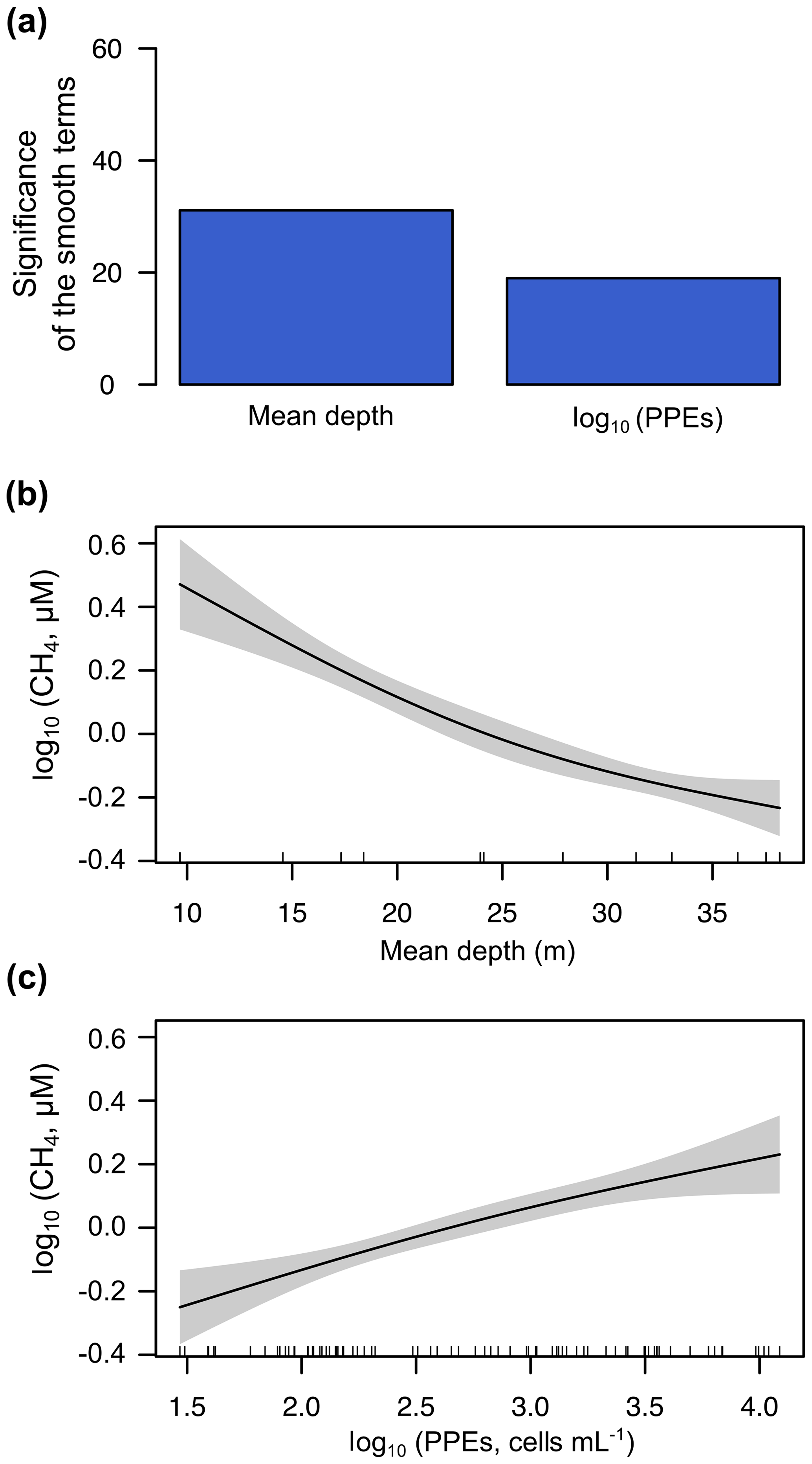
https://www.biogeosciences.net/17/3223/2020/bg-17-3223-2020-f10

Figure 10Results of the generalized additive model (GAM) fitted for the concentrations of CH₄ in the oxic waters during the mixing period. (a) Bar plot showing the significance of the smooth terms from the fitted GAM (F values). Panels (b) and (c) show partial response plots from the fitted GAM, showing the additive effects of the covariates on the dissolved CH₄ concentration: the mean depth (b) and the abundance of photosynthetic picoeukaryotes (log₁₀ PPEs) (c). In partial response plots, the lines are the smoothing functions, and the shaded areas represent 95 % pointwise confidence intervals. Rugs on x axis indicate the distribution of the data. More details are provided in Table S3.

Download

Overall, during the stratification period, the in situ CH₄ production was coupled to the abundance of photosynthetic picoeukaryotes in oxic waters (Fig. 9a) and mean depths. This CH₄ source, due to photosynthetic picoeukaryotes, can be crucial in large, deep lakes and reservoirs and the open ocean, since the impact of the CH₄ transport from sediments (i.e., mean depth) decreases with increasing depths. In deeper reservoirs, the thermal stratification during the summer that produced the vertical diffusion rates of CH₄ from sediments is limited. Rudd and Hamilton (1978) did not detect any movement of CH₄ upwards from the hypolimnion during the stratification. Previous studies have suggested that the CH₄ produced in the oxic water column is the primary source of CH₄ in large and deep lakes (Bogard et al., 2014; DelSontro et al., 2018; Donis et al., 2017; Günthel et al., 2019). Günthel et al. (2019) showed that large lakes have a lower sediment area in comparison to the volume of the surface mixed layer than small lakes and that this fact determines the higher contribution of the oxic methane production to surface emission in large (>1 km²) lakes than in small ones. The photosynthetic picoeukaryotes identified in the studied reservoirs are considered indicators of eutrophic conditions, and they are bloom-forming genera (i.e., Chlorococcales and Chrysochromulina spp.) (Edvardsen and Paasche, 1998; Reynolds, 1984; Willén, 1987). Global future estimations suggest a rise in eutrophication and algal bloom over the next century due to climate change and the growing human population (Beaulieu et al., 2019). In that situation, photosynthetic picoeukaryotes like Chlorococcales and Chrysochromulina spp., and cyanobacteria, would lead to an increment in CH₄ production and emissions. Further studies are needed to understand the role of the photosynthetic picoeukaryotes in the production of CH₄ in oxic waters better and to quantify their influence in the methane supersaturation and CH₄ fluxes from inland and oceanic waters.

4 Conclusions

The dissolved CH₄ concentration in the studied reservoirs showed a considerable variability (i.e., up to 4 orders of magnitude) and presented a clear seasonality. Surface waters were always supersaturated in CH₄. The concentration of CH₄ was closely linked to the photosynthetic organisms. In the anoxic waters, the depth-cumulative chlorophyll a concentration, a proxy for the phytoplanktonic biomass exported to sediments, determined the CH₄ concentration. In the oxic waters, we considered different potential CH₄ sources, including the vertical and lateral transport of CH₄ from anoxic zones and in situ production. The mean depth of the reservoirs, as a surrogate of the CH₄ transport from sediment to the oxic waters, contributed in shallow systems. We did not detect methanogenic Archaea or methylphosphonates degradation target genes (i.e., mcrA and phnJ genes, respectively), which suggests that these pathways are not responsible for the in situ production of CH₄ in the oxic waters of the studied reservoirs. We found that dissolved CH₄ was coupled to the abundance of photosynthetic picoeukaryotes (PPEs) during both periods and to chlorophyll a concentration and the abundance of and cyanobacteria during the stratification period. These PPEs were non-colonial green algae from the order Chlorococcales (class Chlorophyceae, phylum Chlorophyta) and the genus Chrysochromulina spp. (class Coccolithophyceae, phylum Haptophyta). Finally, we combined all the explanatory variables with significant effects and determined their relative contribution to the CH₄ concentration using generalized additive models (GAMs). The abundance of PPEs was the variable explaining most of the variance of dissolved CH₄ concentration during the stratification period, with an effect higher than the cyanobacteria abundance. During the mixing period, the reservoir mean depth and the abundance of the PPEs were the only drivers for CH₄ concentration. Our findings show that the abundance of PPEs can be relevant for explaining the dissolved CH₄ concentration in oxic waters of large lakes and reservoirs.

Data availability

Additional figures and tables can be found in the Supplement. The dataset associated with this paper will be available from PANGAEA (León-Palmero et al., 2020): dissolved concentrations of CH₄, nutrients, and biological parameters in the water column of 12 Mediterranean reservoirs in Southern Spain (https://doi.org/10.1594/PANGAEA.912535, last access: 14 May 2020, and primary production of 12 Mediterranean reservoirs in southern Spain (https://doi.org/10.1594/PANGAEA.912555, last access: 14 May 2020).

Supplement

The supplement related to this article is available online at: https://doi.org/10.5194/bg-17-3223-2020-supplement.

Author contributions

ELP, RMB, and IR contributed equally to this work. RMB and IR designed the study and obtained the funds. ELP, RMB, and IR contributed to data acquisition during the reservoir samplings. ELP processed most of the chemical and biological samples. ACR performed the flow cytometry and part of the molecular analysis, and AS collaborated with the dissolved CH₄ analysis using gas chromatography. ELP, RMB, and IR analyzed the data and discussed the results. ELP wrote the first draft of the paper, which was complemented by significant contributions from RMB and IR.

Competing interests

The authors declare that they have no conflict of interest.

Acknowledgements

We especially thank Eulogio Corral for helping in the field, Jesús Forja and Teodora Ortega for helping with gas chromatography analysis at the University of Cádiz, and David Fernández Moreno from the Department of Botany at the University of Granada for the taxonomical identification of the phytoplankton community. We thank the Hydrological Confederations of Guadalquivir and the Agencia Andaluza del Medio Ambiente y Agua (AMAYA) for facilitating the reservoir sampling.

Financial support

This research has been supported by the Spanish Ministry of Economy and Competitiveness (grant no. CGL2014-52362-R); the University of Granada – Unidades de Excelencia (grant no. UCE.PP2017.03); the Consejería de Economía, Conocimiento, Empresas, y Universidad from Andalucia; and the European Regional Development Fund (ERDF; grant no. SOMM17/6109/UGR). Elizabeth León-Palmero and Ana Sierra were supported by PhD fellowships from the Ministry of Education, Culture and Sport (grant nos. FPU014/02917 and FPU2014-04048, respectively). Alba Contreras-Ruiz was supported by the Youth Employment Initiative (YEI) from the Junta de Andalucía and financed by the European Commission (grant no. 6017).

Review statement

This paper was edited by Carolin Löscher and reviewed by three anonymous referees.

References

Althoff, F., Benzing, K., Comba, P., McRoberts, C., Boyd, D. R., Greiner, S., and Keppler, F.: Abiotic methanogenesis from organosulphur compounds under ambient conditions, Nat. Commun., 5, 4205, https://doi.org/10.1038/ncomms5205, 2014.

Álvarez-Salgado, X. A. and Miller, A. E. J.: Simultaneous determination of dissolved organic carbon and total dissolved nitrogen in seawater by high temperature catalytic oxidation: conditions for precise shipboard measurements, Mar. Chem., 62, 325–333, https://doi.org/10.1016/S0304-4203(98)00037-1, 1998.

American Public Health Association (APHA): Standard methods for the examination of water and wastewater. 1992, 18th ed., edited by: Greenberg, A. E., Clesceri, L. S., and Eaton, A. D., American Public Health Association, Washington, DC, USA., 1100 pp., 1992.

Angel, R., Matthies, D., and Conrad, R.: Activation of Methanogenesis in Arid Biological Soil Crusts Despite the Presence of Oxygen, PLOS ONE, 6, e20453, https://doi.org/10.1371/journal.pone.0020453, 2011.

Angle, J. C., Morin, T. H., Solden, L. M., Narrowe, A. B., Smith, G. J., Borton, M. A., Rey-Sanchez, C., Daly, R. A., Mirfenderesgi, G., Hoyt, D. W., Riley, W. J., Miller, C. S., Bohrer, G., and Wrighton, K. C.: Methanogenesis in oxygenated soils is a substantial fraction of wetland methane emissions, Nat. Commun., 8, 1–9, https://doi.org/10.1038/s41467-017-01753-4, 2017.

Aronow, S.: Shoreline development ratio, in Beaches and Coastal Geology, Springer US, Boston, MA, 754–755, 1982.

Axler, R. P., Rose, C., and Tikkanen, C. A.: Phytoplankton Nutrient Deficiency as Related to Atmospheric Nitrogen Deposition in Northern Minnesota Acid-Sensitive Lakes, Can. J. Fish. Aquat. Sci., 51, 1281–1296, https://doi.org/10.1139/f94-128, 1994.

Bastviken, D., Cole, J., Pace, M., and Tranvik, L.: Methane emissions from lakes: Dependence of lake characteristics, two regional assessments, and a global estimate, Glob. Biogeochem. Cy., 18, 1–12, https://doi.org/10.1029/2004GB002238, 2004.

Bastviken, D., Tranvik, L. J., Downing, J. A., Crill, P. M., and Enrich-Prast, A.: Freshwater Methane Emissions Offset the Continental Carbon Sink, Science, 331, 1–12, https://doi.org/10.1126/science.1196808, 2011.

Beaulieu, J. J., DelSontro, T., and Downing, J. A.: Eutrophication will increase methane emissions from lakes and impoundments during the 21st century, Nat. Commun., 10, 1375, https://doi.org/10.1038/s41467-019-09100-5, 2019.

Berg, A., Lindblad, P., and Svensson, B. H.: Cyanobacteria as a source of hydrogen for methane formation, World J. Microbiol. Biotechnol., 30, 539–545, https://doi.org/10.1007/s11274-013-1463-5, 2014.

Berg, I. A.: Ecological Aspects of the Distribution of Different Autotrophic CO₂ Fixation Pathways, Appl. Environ. Microbiol., 77, 1925–1936, https://doi.org/10.1128/AEM.02473-10, 2011.

Beversdorf, L. J., White, A. E., Björkman, K. M., Letelier, R. M., and Karl, D. M.: Phosphonate metabolism by Trichodesmium IMS101 and the production of greenhouse gases, Limnol. Oceanogr., 55, 1768–1778, https://doi.org/10.4319/lo.2010.55.4.1768, 2010.

Bižić, M., Klintzsch, T., Ionescu, D., Hindiyeh, M. Y., Günthel, M., Muro-Pastor, A. M., Eckert, W., Urich, T., Keppler, F., and Grossart, H.-P.: Aquatic and terrestrial cyanobacteria produce methane, Sci. Adv., 6: eaax5343, https://doi.org/10.1126/sciadv.aax5343, 2020.

Bižić-Ionescu, M., Ionescu, D., Günthel, M., Tang, K. W., and Grossart, H. P.: Oxic methane cycling: New evidence for methane formation in Oxic lake water, in: Biogenesis of Hydrocarbons, edited by: Stams, A. J. M. and Souna, D. Z., Springer International Publishing, Basel, 1–22, 2018.

Blees, J., Niemann, H., Erne, M., Zopfi, J., Schubert, C. J., and Lehmann, M. F.: Spatial variations in surface water methane super-saturation and emission in Lake Lugano, southern Switzerland, Aquat. Sci., 77, 535–545, https://doi.org/10.1007/s00027-015-0401-z, 2015.

Bogard, M. J., del Giorgio, P. A., Boutet, L., Chaves, M. C. G., Prairie, Y. T., Merante, A., and Derry, A. M.: Oxic water column methanogenesis as a major component of aquatic CH4 fluxes, Nat. Commun., 5, 5350, https://doi.org/10.1038/ncomms6350, 2014.

Boström, K. H., Simu, K., Hagström, Å., and Riemann, L.: Optimization of DNA extraction for quantitative marine bacterioplankton community analysis, Limnol. Oceanogr. Method., 2, 365–373, https://doi.org/10.4319/lom.2004.2.365, 2004.

Burns, B. D. and Beardall, J.: Utilization of inorganic carbon by marine microalgae, J. Exp. Mar. Biol. Ecol., 107, 75–86, https://doi.org/10.1016/0022-0981(87)90125-0, 1987.

Carini, P., White, A. E., Campbell, E. O., and Giovannoni, S. J.: Methane production by phosphate-starved SAR11 chemoheterotrophic marine bacteria, Nat. Commun., 5, 4346, https://doi.org/10.1038/ncomms5346, 2014.

Cellamare, M., Rolland, A., and Jacquet, S.: Flow cytometry sorting of freshwater phytoplankton, J. Appl. Phycol., 22, 87–100, https://doi.org/10.1007/s10811-009-9439-4, 2010.

Chistoserdova, L., Vorholt, J. A., Thauer, R. K., and Lidstrom, M. E.: C1 Transfer Enzymes and Coenzymes Linking Methylotrophic Bacteria and Methanogenic Archaea, Science, 281, 99–102, https://doi.org/10.1126/science.281.5373.99, 1998.

Cole, J. J., Pace, M. L., Carpenter, S. R., and Kitchell, J. F.: Persistence of net heterotrophy in lakes during nutrient addition and food web manipulations, Limnol. Oceanogr., 45, 1718–1730, https://doi.org/10.4319/lo.2000.45.8.1718, 2000.

Collier, J. L.: Flow Cytometry and the Single Cell in Phycology, J. Appl. Phycol., 36, 628–644, https://doi.org/10.1046/j.1529-8817.2000.99215.x, 2000.

Corzo, A., Jimenez-Gomez, F., Gordillo, F., Garcia-Ruiz, R., and Niell, F.: Synechococcus and Prochlorococcus-like populations detected by flow cytometry in a eutrophic reservoir in summer, J. Plankton Res., 21, 1575–1581, https://doi.org/10.1093/plankt/21.8.1575, 1999.

Crowe, S. A., O'Neill, A. H., Katsev, S., Hehanussa, P., Haffner, G. D., Sundby, B., Mucci, A., and Fowle, D. A.: The biogeochemistry of tropical lakes: A case study from Lake Matano, Indonesia, Limnol. Oceanogr., 53, 319–331, https://doi.org/10.4319/lo.2008.53.1.0319, 2008.

Damm, E., Kiene, R. P., Schwarz, J., Falck, E., and Dieckmann, G.: Methane cycling in Arctic shelf water and its relationship with phytoplankton biomass and DMSP, Mar. Chem., 109, 45–59, https://doi.org/10.1016/j.marchem.2007.12.003, 2008.

Damm, E., Helmke, E., Thoms, S., Schauer, U., Nöthig, E., Bakker, K., and Kiene, R. P.: Methane production in aerobic oligotrophic surface water in the central Arctic Ocean, Biogeosciences, 7, 1099–1108, https://doi.org/10.5194/bg-7-1099-2010, 2010.

Damm, E., Thoms, S., Beszczynska-Möller, A., Nöthig, E. M., and Kattner, G.: Methane excess production in oxygen-rich polar water and a model of cellular conditions for this paradox, Polar Sci., 9, 327–334, https://doi.org/10.1016/j.polar.2015.05.001, 2015.

de Angelis, M. A. and Lee, C.: Methane production during zooplankton grazing on marine phytoplankton, Limnol. Oceanogr., 39, 1298–1308, https://doi.org/10.4319/lo.1994.39.6.1298, 1994.

Deemer, B. R., Harrison, J. A., Li, S., Beaulieu, J. J., DelSontro, T., Barros, N., Bezerra-Neto, J. F., Powers, S. M., dos Santos, M. A., and Vonk, J. A.: Greenhouse Gas Emissions from Reservoir Water Surfaces: A New Global Synthesis, BioScience, 66, 949–964, https://doi.org/10.1093/biosci/biw117, 2016.

DelSontro, T., del Giorgio, P. A., and Prairie, Y. T.: No Longer a Paradox: The Interaction Between Physical Transport and Biological Processes Explains the Spatial Distribution of Surface Water Methane Within and Across Lakes, Ecosystems, 21, 1073–1087, https://doi.org/10.1007/s10021-017-0205-1, 2018.

del Valle, D. A. and Karl, D. M.: Aerobic production of methane from dissolved water-column methylphosphonate and sinking particles in the North Pacific Subtropical Gyre, Aquat. Microb. Ecol., 73, 93–105, https://doi.org/10.3354/ame01714, 2014.

Dlugokencky, E. J.: Trends in Atmospheric Methane. Globally averaged marine surface monthly mean data, NOAA/ESRL, available at: https://www.esrl.noaa.gov/gmd/ccgg/trends_ch4/, last access: 29 July 2019.

Donis, D., Flury, S., Stöckli, A., Spangenberg, J. E., Vachon, D., and McGinnis, D. F.: Full-scale evaluation of methane production under oxic conditions in a mesotrophic lake, Nat. Commun., 8, 1661, https://doi.org/10.1038/s41467-017-01648-4, 2017.

Edvardsen, B. and Paasche, E.: Bloom dynamics and physiology of Prymnesium and Chrysochromulina, Nato Asi. Ser. G. Ecol. Sci., 41, 193–208, 1998.

Encinas Fernández, J., Peeters, F., and Hofmann, H.: On the methane paradox: Transport from shallow water zones rather than in situ methanogenesis is the major source of CH₄ in the open surface water of lakes, JGR: Biogeosciences, 121, 2717–2726, https://doi.org/10.1002/2016JG003586, 2016.

Fox, A., Kwapinski, W., Griffiths, B. S., and Schmalenberger, A.: The role of sulfur- and phosphorus-mobilizing bacteria in biochar-induced growth promotion of Lolium perenne, FEMS Microbiol. Ecol., 90, 78–91, https://doi.org/10.1111/1574-6941.12374, 2014.

Fox, J. and Weisberg, S.: An R Companion to Applied Regression, Second., Sage, Thousand Oaks CA, available at: http://socserv.socsci.mcmaster.ca/jfox/Books/Companion (last access: 3 June 2018), 2011.

Gasol, J. M. and del Giorgio, P. A.: Using flow cytometry for counting natural planktonic bacteria and understanding the structure of planktonic bacterial communities, Sci. Mar., 64, 197–224, https://doi.org/10.3989/scimar.2000.64n2197, 2000.

Gomez-Garcia, M. R., Davison, M., Blain-Hartnung, M., Grossman, A. R., and Bhaya, D.: Alternative pathways for phosphonate metabolism in thermophilic cyanobacteria from microbial mats, ISME J., 5, 141–149, https://doi.org/10.1038/ismej.2010.96, 2011.

Grabarse, W., Mahlert, F., Duin, E. C., Goubeaud, M., Shima, S., Thauer, R. K., Lamzin, V., and Ermler, U.: On the mechanism of biological methane formation: structural evidence for conformational changes in methyl-coenzyme M reductase upon substrate binding, J. Mol. Biol., 309, 315–330, https://doi.org/10.1006/jmbi.2001.4647, 2001.

Gross, J. and Ligges, U.: nortest: Tests for Normality, available at: https://CRAN.R-project.org/package=nortest (last access: 3 June 2018), 2015.

Grossart, H.-P., Frindte, K., Dziallas, C., Eckert, W., and Tang, K. W.: Microbial methane production in oxygenated water column of an oligotrophic lake, P. Natl. Acad. Sci. USA, 108, 19657–19661, https://doi.org/10.1073/pnas.1110716108, 2011.

Günthel, M., Donis, D., Kirillin, G., Ionescu, D., Bizic, M., McGinnis, D. F., Grossart, H.-P., and Tang, K. W.: Contribution of oxic methane production to surface methane emission in lakes and its global importance, Nat. Commun., 10, 1–10, https://doi.org/10.1038/s41467-019-13320-0, 2019.

Hartmann, J. F., Günthel, M., Klintzsch, T., Kirillin, G., Grossart, H.-P., Keppler, F., and Isenbeck-Schröter, M.: High Spatiotemporal Dynamics of Methane Production and Emission in Oxic Surface Water, Environ. Sci. Technol., 54, 1451–1463, https://doi.org/10.1021/acs.est.9b03182, 2020.

Hastie, T. and Tibshirani, R.: Generalized Additive Models, Statist. Sci., 1, 297–310, https://doi.org/10.1214/ss/1177013604, 1986.

Hastie, T. and Tibshirani, R. J.: Generalized additive models, London, Chapman and Hall, 335 pp., 1990.

Hofmann, H., Federwisch, L., and Peeters, F.: Wave-induced release of methane: Littoral zones as source of methane in lakes, Limnol. Oceanogr., 55, 1990–2000, https://doi.org/10.4319/lo.2010.55.5.1990, 2010.

Jähne, B., Münnich, K. O., Bösinger, R., Dutzi, A., Huber, W., and Libner, P.: On the parameters influencing air-water gas exchange, J. Geophys. Res.-Ocean., 92, 1937–1949, https://doi.org/10.1029/JC092iC02p01937, 1987.

Jarrell, K. F.: Extreme Oxygen Sensitivity in Methanogenic Archaebacteria, BioScience, 35, 298–302, https://doi.org/10.2307/1309929, 1985.

Karl, D. M. and Tilbrook, B. D.: Production and transport of methane in oceanic particulate organic matter, Nature, 368, 732–734, https://doi.org/10.1038/368732a0, 1994.

Karl, D. M., Beversdorf, L., Björkman, K. M., Church, M. J., Martinez, A., and Delong, E. F.: Aerobic production of methane in the sea, Nat. Geosci., 1, 473–478, https://doi.org/10.1038/ngeo234, 2008.

Khatun, S., Iwata, T., Kojima, H., Fukui, M., Aoki, T., Mochizuki, S., Naito, A., Kobayashi, A., and Uzawa, R.: Aerobic methane production by planktonic microbes in lakes, Sci. Total Environ., 696, 133916, https://doi.org/10.1016/j.scitotenv.2019.133916, 2019.

Khatun, S., Iwata, T., Kojima, H., Ikarashi, Y., Yamanami, K., Imazawa, D., Kenta, T., Shinohara, R., and Saito, H.: Linking Stoichiometric Organic Carbon–Nitrogen Relationships to planktonic Cyanobacteria and Subsurface Methane Maximum in Deep Freshwater Lakes, Water, 12, 402, https://doi.org/10.3390/w12020402, 2020.

Kiene, R. P.: Production and consumption of methane in aquatic systems, in Microbial Production and Consumption of Greenhouse Gases: Methane, Nitrogen Oxides, and Halomethanes, edited by: Rogers, J. E. and Whitman, W. B., American Society for Microbiology, Washington, DC, USA, 111–146, 1991.

Klintzsch, T., Langer, G., Nehrke, G., Wieland, A., Lenhart, K., and Keppler, F.: Methane production by three widespread marine phytoplankton species: release rates, precursor compounds, and potential relevance for the environment, Biogeosciences, 16, 4129–4144, https://doi.org/10.5194/bg-16-4129-2019, 2019.

Lenhart, K., Bunge, M., Ratering, S., Neu, T. R., Schüttmann, I., Greule, M., Kammann, C., Schnell, S., Müller, C., Zorn, H., and Keppler, F.: Evidence for methane production by saprotrophic fungi, Nat. Commun., 3, 1046, https://doi.org/10.1038/ncomms2049, 2012.

Lenhart, K., Althoff, F., Greule, M., and Keppler, F.: Technical Note: Methionine, a precursor of methane in living plants, Biogeosciences, 12, 1907–1914, https://doi.org/10.5194/bg-12-1907-2015, 2015.

Lenhart, K., Klintzsch, T., Langer, G., Nehrke, G., Bunge, M., Schnell, S., and Keppler, F.: Evidence for methane production by the marine algae Emiliania huxleyi, Biogeosciences, 13, 3163–3174, https://doi.org/10.5194/bg-13-3163-2016, 2016.

León-Palmero, E., Reche, I., and Morales-Baquero, R.: Atenuación de luz en embalses del sur-este de la Península Ibérica, Ingeniería del agua, 23, 65–75, https://doi.org/10.4995/ia.2019.10655, 2019.

León-Palmero, E., Morales-Baquero, R., and Reche, I.: Greenhouse gas fluxes from reservoirs determined by watershed lithology, morphometry, and anthropogenic pressure, Environ. Res. Lett., 15, 044012, https://doi.org/10.1088/1748-9326/ab7467, 2020.

Liu, H., Jing, H., Wong, T. H. C., and Chen, B.: Co-occurrence of phycocyanin- and phycoerythrin-rich Synechococcus in subtropical estuarine and coastal waters of Hong Kong, Environ. Microbiol. Rep., 6, 90–99, https://doi.org/10.1111/1758-2229.12111, 2014.

Marotta, H., Pinho, L., Gudasz, C., Bastviken, D., Tranvik, L. J., and Enrich-Prast, A.: Greenhouse gas production in low-latitude lake sediments responds strongly to warming, Nat. Clim. Change, 4, 467–470, https://doi.org/10.1038/nclimate2222, 2014.

Michmerhuizen, C. M., Striegl, R. G., and McDonald, M. E.: Potential methane emission from north-temperate lakes following ice melt, Limnol. Oceanogr., 41, 985–991, https://doi.org/10.4319/lo.1996.41.5.0985, 1996.

Mitsch, W. J., Bernal, B., Nahlik, A. M., Mander, Ü., Zhang, L., Anderson, C. J., Jørgensen, S. E., and Brix, H.: Wetlands, carbon, and climate change, Landsc. Ecol., 28, 583–597, https://doi.org/10.1007/s10980-012-9758-8, 2012.

Morris, D. P. and Lewis, W. M.: Phytoplankton nutrient limitation in Colorado mountain lakes, Freshw. Biol., 20, 315–327, https://doi.org/10.1111/j.1365-2427.1988.tb00457.x, 1988.

Mortimer, C. H.: The oxygen content of air-saturated fresh waters, and aids in calculating percentage saturation, Schweizerbart Science Publishers, Stuttgart, Germany, available at: http://www.schweizerbart.de//publications/detail/isbn/9783510520060/Mitteilungen_IVL_Nr_6 (last access: 25 November 2017), 1956.

Murase, J. and Sugimoto, A.: Inhibitory effect of light on methane oxidation in the pelagic water column of a mesotrophic lake (Lake Biwa, Japan), Limnol. Oceanogr., 50, 1339–1343, https://doi.org/10.4319/lo.2005.50.4.1339, 2005.

Murase, J., Sakai, Y., Sugimoto, A., Okubo, K., and Sakamoto, M.: Sources of dissolved methane in Lake Biwa, Limnology, 4, 91–99, https://doi.org/10.1007/s10201-003-0095-0, 2003.

Murphy, J. and Riley, J. P.: A modified single solution method for the determination of phosphate in natural waters, Anal. Chim. Acta, 27, 31–36, https://doi.org/10.1016/S0003-2670(00)88444-5, 1962.

Musenze, R. S., Grinham, A., Werner, U., Gale, D., Sturm, K., Udy, J., and Yuan, Z.: Assessing the spatial and temporal variability of diffusive methane and nitrous oxide emissions from subtropical freshwater reservoirs, Environ. Sci. Technol., 48, 14499–14507, https://doi.org/10.1021/es505324h, 2014.

Naqvi, S. W. A., Lam, P., Narvenkar, G., Sarkar, A., Naik, H., Pratihary, A., Shenoy, D. M., Gauns, M., Kurian, S., Damare, S., Duret, M., Lavik, G., and Kuypers, M. M. M.: Methane stimulates massive nitrogen loss from freshwater reservoirs in India, Nat. Commun., 9, 1–10, https://doi.org/10.1038/s41467-018-03607-z, 2018.

Odum, H. T.: Primary Production in Flowing Waters, Limnol. Oceanogr., 1, 102–117, https://doi.org/10.4319/lo.1956.1.2.0102, 1956.

Okuku, E. O., Bouillon, S., Tole, M., and Borges, A. V.: Diffusive emissions of methane and nitrous oxide from a cascade of tropical hydropower reservoirs in Kenya, Lakes Reserv. Res. Manag., 24, 127–135, https://doi.org/10.1111/lre.12264, 2019.

Oswald, K., Milucka, J., Brand, A., Littmann, S., Wehrli, B., Kuypers, M. M. M., and Schubert, C. J.: Light-Dependent Aerobic Methane Oxidation Reduces Methane Emissions from Seasonally Stratified Lakes, PLoS One, 10, e0132574–e0132574, doi:10.1371/journal.pone.0132574, 2015.

Oswald, K., Jegge, C., Tischer, J., Berg, J., Brand, A., Miracle, M. R., Soria, X., Vicente, E., Lehmann, M. F., Zopfi, J., and Schubert, C. J.: Methanotrophy under Versatile Conditions in the Water Column of the Ferruginous Meromictic Lake La Cruz (Spain), Front. Microbiol., 7, 1762 pp., https://doi.org/10.3389/fmicb.2016.01762, 2016.

Owens, N. J. P., Law, C. S., Mantoura, R. F. C., Burkill, P. H., and Llewellyn, C. A.: Methane flux to the atmosphere from the Arabian Sea, Nature, 354, 293–296, https://doi.org/10.1038/354293a0, 1991.

Peeters, F., Wüest, A., Piepke, G., and Imboden, D. M.: Horizontal mixing in lakes, J. Geophys. Res.-Ocean., 101, 18361–18375, https://doi.org/10.1029/96JC01145, 1996.

Peeters, F., Fernandez Encinas, J., and Hofmann, H.: Sediment fluxes rather than oxic methanogenesis explain diffusive CH₄ emissions from lakes and reservoirs, Sci. Rep., 9, 1–10, https://doi.org/10.1038/s41598-018-36530-w, 2019.

R Core Team: R: A Language and Environment for Statistical Computing, R Foundation for Statistical Computing, Vienna, Austria, available at: http://www.R-project.org/, (last access: 20 February 2020) 2014.

Rasilo, T., Prairie, Y. T., and del Giorgio, P. A.: Large-scale patterns in summer diffusive CH₄ fluxes across boreal lakes, and contribution to diffusive C emissions, Glob. Change Biol., 21, 1124–1139, https://doi.org/10.1111/gcb.12741, 2015.

Repeta, D. J., Ferrón, S., Sosa, O. A., Johnson, C. G., Repeta, L. D., Acker, M., DeLong, E. F., and Karl, D. M.: Marine methane paradox explained by bacterial degradation of dissolved organic matter, Nat. Geosci., 9, 884–887, https://doi.org/10.1038/ngeo2837, 2016.

Reynolds, C. S.: Phytoplankton periodicity: the interactions of form, function and environmental variability, Freshw. Biol., 14, 111–142, https://doi.org/10.1111/j.1365-2427.1984.tb00027.x, 1984.

Roland, F. A. E., Darchambeau, F., Morana, C., and Borges, A. V.: Nitrous oxide and methane seasonal variability in the epilimnion of a large tropical meromictic lake (Lake Kivu, East-Africa), Aquat. Sci., 79, 209–218, https://doi.org/10.1007/s00027-016-0491-2, 2017.

Rudd, J. W. M. and Hamilton, R. D.: Methane cycling in a eutrophic shield lake and its effects on whole lake metabolism, Limnol. Oceanogr., 23, 337–348, https://doi.org/10.4319/lo.1978.23.2.0337, 1978.

Sabo, E., Roy, D., Hamilton, P. B., Hehanussa, P. E., McNeely, R., and Haffner, G. D.: The plankton community of Lake Matano: factors regulating plankton composition and relative abundance in an ancient, tropical lake of Indonesia, in: Patterns and Processes of Speciation in Ancient Lakes, Springer, 225–235, 2008.

Saunois, M., Bousquet, P., Poulter, B., Peregon, A., Ciais, P., Canadell, J. G., Dlugokencky, E. J., Etiope, G., Bastviken, D., Houweling, S., Janssens-Maenhout, G., Tubiello, F. N., Castaldi, S., Jackson, R. B., Alexe, M., Arora, V. K., Beerling, D. J., Bergamaschi, P., Blake, D. R., Brailsford, G., Brovkin, V., Bruhwiler, L., Crevoisier, C., Crill, P., Covey, K., Curry, C., Frankenberg, C., Gedney, N., Höglund-Isaksson, L., Ishizawa, M., Ito, A., Joos, F., Kim, H.-S., Kleinen, T., Krummel, P., Lamarque, J.-F., Langenfelds, R., Locatelli, R., Machida, T., Maksyutov, S., McDonald, K. C., Marshall, J., Melton, J. R., Morino, I., Naik, V., O'Doherty, S., Parmentier, F.-J. W., Patra, P. K., Peng, C., Peng, S., Peters, G. P., Pison, I., Prigent, C., Prinn, R., Ramonet, M., Riley, W. J., Saito, M., Santini, M., Schroeder, R., Simpson, I. J., Spahni, R., Steele, P., Takizawa, A., Thornton, B. F., Tian, H., Tohjima, Y., Viovy, N., Voulgarakis, A., van Weele, M., van der Werf, G. R., Weiss, R., Wiedinmyer, C., Wilton, D. J., Wiltshire, A., Worthy, D., Wunch, D., Xu, X., Yoshida, Y., Zhang, B., Zhang, Z., and Zhu, Q.: The global methane budget 2000–2012, Earth Syst. Sci. Data, 8, 697–751, https://doi.org/10.5194/essd-8-697-2016, 2016.

Schlesinger, W. H. and Bernhardt, E. S.: Biogeochemistry: An Analysis of Global Change, Academic Press, 689 pp., 2013.

Schmale, O., Wäge, J., Mohrholz, V., Wasmund, N., Gräwe, U., Rehder, G., Labrenz, M., and Loick-Wilde, N.: The contribution of zooplankton to methane supersaturation in the oxygenated upper waters of the central Baltic Sea, Limnol. Oceanogr., 63, 412–430, https://doi.org/10.1002/lno.10640, 2018.

Schmidt, U. and Conrad, R.: Hydrogen, carbon monoxide, and methane dynamics in Lake Constance, Limnol. Oceanogr., 38, 1214–1226, https://doi.org/10.4319/lo.1993.38.6.1214, 1993.

Schubert, C. J. and Wehrli, B.: Contribution of Methane Formation and Methane Oxidation to Methane Emission from Freshwater Systems, in: Biogenesis of Hydrocarbons, edited by: Stams, A. J. M. and Sousa, D., Springer International Publishing, Cham., 1–31, 2018.

Schulz, M., Faber, E., Hollerbach, A., Schröder, H. G., and Güde, H.: The methane cycle in the epilimnion of Lake Constance, Archiv Hydrobiol., 157–176, https://doi.org/10.1127/archiv-hydrobiol/151/2001/157, 2001.

Schwarz, J. I. K., Eckert, W., and Conrad, R.: Response of the methanogenic microbial community of a profundal lake sediment (Lake Kinneret, Israel) to algal deposition, Limnol. Oceanogr., 53, 113–121, https://doi.org/10.4319/lo.2008.53.1.0113, 2008.

Scranton, M. I. and Brewer, P. G.: Occurrence of methane in the near-surface waters of the western subtropical North-Atlantic, Deep-Sea Res., 24, 127–138, https://doi.org/10.1016/0146-6291(77)90548-3, 1977.

Segers, R.: Methane production and methane consumption: a review of processes underlying wetland methane fluxes, Biogeochemistry, 41, 23–51, https://doi.org/10.1023/A:1005929032764, 1998.

Sepulveda-Jauregui, A., Hoyos-Santillan, J., Martinez-Cruz, K., Walter Anthony, K. M., Casper, P., Belmonte-Izquierdo, Y., and Thalasso, F.: Eutrophication exacerbates the impact of climate warming on lake methane emission, Sci. Total Environ., 636, 411–419, https://doi.org/10.1016/j.scitotenv.2018.04.283, 2018.

Seweryn, P., Van, L. B., Kjeldgaard, M., Russo, C. J., Passmore, L. A., Hove-Jensen, B., Jochimsen, B., and Brodersen, D. E.: Structural insights into the bacterial carbon-phosphorus lyase machinery, Nature, 525, 68–72, https://doi.org/10.1038/nature14683, 2015.

Shaw, S. L., Chisholm, S. W., and Prinn, R. G.: Isoprene production by Prochlorococcus, a marine cyanobacterium, and other phytoplankton, Mar. Chem., 80, 227–245, https://doi.org/10.1016/S0304-4203(02)00101-9, 2003.

Sierra, A., Jiménez-López, D., Ortega, T., Ponce, R., Bellanco, M. J., Sánchez-Leal, R., Gómez-Parra, A., and Forja, J.: Spatial and seasonal variability of CH₄ in the eastern Gulf of Cadiz (SW Iberian Peninsula), Sci. Total Environ., 590/591, 695–707, https://doi.org/10.1016/j.scitotenv.2017.03.030, 2017.

Staehr, P. A., Bade, D., Bogert, M. C. V. de, Koch, G. R., Williamson, C., Hanson, P., Cole, J. J., and Kratz, T.: Lake metabolism and the diel oxygen technique: State of the science, Limnol. Oceanogr.-Method., 8, 628–644, https://doi.org/10.4319/lom.2010.8.0628, 2010.

Steinke, M., Hodapp, B., Subhan, R., Bell, T. G., and Martin-Creuzburg, D.: Flux of the biogenic volatiles isoprene and dimethyl sulfide from an oligotrophic lake, Sci. Rep., 8, 1–10, https://doi.org/10.1038/s41598-017-18923-5, 2018.

Tang, K. W., McGinnis, D. F., Frindte, K., Brüchert, V., and Grossart, H.-P.: Paradox reconsidered: Methane oversaturation in well-oxygenated lake waters, Limnol. Oceanogr., 59, 275–284, https://doi.org/10.4319/lo.2014.59.1.0275, 2014.

Tang, K. W., McGinnis, D. F., Ionescu, D., and Grossart, H.-P.: Methane Production in Oxic Lake Waters Potentially Increases Aquatic Methane Flux to Air, Environ. Sci. Technol. Lett., 3, 227–233, https://doi.org/10.1021/acs.estlett.6b00150, 2016.

Teikari, J. E., Fewer, D. P., Shrestha, R., Hou, S., Leikoski, N., Mäkelä, M., Simojoki, A., Hess, W. R., and Sivonen, K.: Strains of the toxic and bloom-forming Nodularia spumigena (cyanobacteria) can degrade methylphosphonate and release methane, ISME J., 12, 1619–1630, https://doi.org/10.1038/s41396-018-0056-6, 2018.

Thalasso, F., Sepulveda-Jauregui, A., Gandois, L., Martinez-Cruz, K., Gerardo-Nieto, O., Astorga-España, M. S., Teisserenc, R., Lavergne, C., Tananaev, N., Barret, M., and Cabrol, L.: Sub-oxycline methane oxidation can fully uptake CH₄ produced in sediments: case study of a lake in Siberia, Sci. Rep., 10, 1–7, https://doi.org/10.1038/s41598-020-60394-8, 2020.

Thanh-Duc, N., Crill, P., and Bastviken, D.: Implications of temperature and sediment characteristics on methane formation and oxidation in lake sediments, Biogeochemistry, 100, 185–196, https://doi.org/10.1007/s10533-010-9415-8, 2010.

Tilbrook, B. D. and Karl, D. M.: Methane sources, distributions and sinks from California coastal waters to the oligotrophic North Pacific gyre, Mar. Chem., 49, 51–64, https://doi.org/10.1016/0304-4203(94)00058-L, 1995.

Wang, Q., Dore, J. E., and McDermott, T. R.: Methylphosphonate metabolism by Pseudomonas sp. populations contributes to the methane oversaturation paradox in an oxic freshwater lake, Environ. Microbiol., 19, 2366–2378, https://doi.org/10.1111/1462-2920.13747, 2017.

West, W. E., Coloso, J. J., and Jones, S. E.: Effects of algal and terrestrial carbon on methane production rates and methanogen community structure in a temperate lake sediment, Freshwater Biol., 57, 949–955, https://doi.org/10.1111/j.1365-2427.2012.02755.x, 2012.

West, W. E., McCarthy, S. M., and Jones, S. E.: Phytoplankton lipid content influences freshwater lake methanogenesis, Freshwater Biol., 60, 2261–2269, https://doi.org/10.1111/fwb.12652, 2015.

West, W. E., Creamer, K. P., and Jones, S. E.: Productivity and depth regulate lake contributions to atmospheric methane: Lake productivity fuels methane emissions, Limnol. Oceanogr., 61, S51–S61, https://doi.org/10.1002/lno.10247, 2016.

White, A. K. and Metcalf, W. W.: Microbial Metabolism of Reduced Phosphorus Compounds, Annu. Rev. Microbiol., 61, 379–400, https://doi.org/10.1146/annurev.micro.61.080706.093357, 2007.

Wiesenburg, D. A. and Guinasso, N. L.: Equilibrium solubilities of methane, carbon monoxide, and hydrogen in water and sea water, J. Chem. Eng. Data, 24, 356–360, https://doi.org/10.1021/je60083a006, 1979.

Willén, E.: Phytoplankton and reversed Eutrophication in Lake Mälaren, Central Sweden, 1965–1983, Br. Phycol. J., 22, 193–208, https://doi.org/10.1080/00071618700650241, 1987.

Wood, S. N.: Generalized additive models: an introduction with R, Chapman and Hall/CRC, New York, USA, 416 pp., 2006.

Wood, S. N.: Fast stable restricted maximum likelihood and marginal likelihood estimation of semiparametric generalized linear models, J. R. Stat. Soc. Ser. B, 73, 3–36, https://doi.org/10.1111/j.1467-9868.2010.00749.x, 2011.

Yamamoto, S., Alcauskas, J. B., and Crozier, T. E.: Solubility of methane in distilled water and seawater, J. Chem. Eng. Data, 21, 78–80, https://doi.org/10.1021/je60068a029, 1976.

Yao, M., Henny, C., and Maresca, J. A.: Freshwater bacteria release methane as a byproduct of phosphorus acquisition, Appl. Environ. Microbiol., 82, 6994–7003, https://doi.org/10.1128/AEM.02399-16, 2016a.

Yao, M., Elling, F. J., Jones, C., Nomosatryo, S., Long, C. P., Crowe, S. A., Antoniewicz, M. R., Hinrichs, K.-U., and Maresca, J. A.: Heterotrophic bacteria from an extremely phosphate-poor lake have conditionally reduced phosphorus demand and utilize diverse sources of phosphorus, Environ. Microbiol., 18, 656–667, https://doi.org/10.1111/1462-2920.13063, 2016b.

Yoch, D. C.: Dimethylsulfoniopropionate: its sources, role in the marine food web, and biological degradation to dimethylsulfide, Appl. Environ. Microbiol., 68, 5804–5815, https://doi.org/10.1128/AEM.68.12.5804-5815.2002, 2002.

Yvon-Durocher, G., Allen, A. P., Bastviken, D., Conrad, R., Gudasz, C., St-Pierre, A., Thanh-Duc, N., and del Giorgio, P. A.: Methane fluxes show consistent temperature dependence across microbial to ecosystem scales, Nature, 507, 488–491, https://doi.org/10.1038/nature13164, 2014.

Zindler, C., Bracher, A., Marandino, C. A., Taylor, B., Torrecilla, E., Kock, A., and Bange, H. W.: Sulphur compounds, methane, and phytoplankton: interactions along a north–south transit in the western Pacific Ocean, Biogeosciences, 10, 3297–3311, https://doi.org/10.5194/bg-10-3297-2013, 2013.

Articles

Download

The requested paper has a corresponding corrigendum published. Please read the corrigendum first before downloading the article.

Article (4667 KB)
Full-text XML

Short summary

CH₄ emissions from reservoirs are responsible for the majority of the climatic forcing of these ecosystems. The origin of the recurrent CH₄ supersaturation in oxic waters is still controversial. We found that the dissolved CH₄ concentration varied by up to 4 orders of magnitude in the water column of 12 reservoirs and was consistently supersaturated. Our findings suggest that photosynthetic picoeukaryotes can play a significant role in determining CH₄ concentration in oxic waters.

Dissolved CH4 coupled to photosynthetic picoeukaryotes in oxic waters and to cumulative chlorophyll a in anoxic waters of reservoirs

2.1 Studied reservoirs, morphometry, and vertical profiles

2.2 Dissolved CH4 in the water column

2.3 Chemical analysis in the water column

2.4 Chlorophyll a, phytoplankton, and primary production in the water column

2.5 DNA analysis

2.6 Statistical tests

3.1 Profile description

3.2 CH4 sources in the water column

3.2.1 CH4 sources in anoxic waters

3.2.2 CH4 sources in oxic waters

Vertical and lateral CH4 transport from anoxic sediments to oxic waters

In situ CH4 production by methanogenic Archaea or methylphosphonate degradation

In situ CH4 production coupled to photosynthetic organisms

3.2.3 Modeling the CH4 production in oxic waters

Dissolved CH₄ coupled to photosynthetic picoeukaryotes in oxic waters and to cumulative chlorophyll a in anoxic waters of reservoirs

2.2 Dissolved CH₄ in the water column

3.2 CH₄ sources in the water column

3.2.1 CH₄ sources in anoxic waters

3.2.2 CH₄ sources in oxic waters

Vertical and lateral CH₄ transport from anoxic sediments to oxic waters

In situ CH₄ production by methanogenic Archaea or methylphosphonate degradation

In situ CH₄ production coupled to photosynthetic organisms

3.2.3 Modeling the CH₄ production in oxic waters