the Creative Commons Attribution 4.0 License.
the Creative Commons Attribution 4.0 License.
 | 19 Mar 2020
A robust data cleaning procedure for eddy covariance flux measurements
Gerardo Fratini
Massimo Bilancia
Giacomo Nicolini
Simone Sabbatini
Dario Papale
The sources of systematic error responsible for introducing significant biases in the eddy covariance (EC) flux computation are manifold, and their correct identification is made difficult by the lack of reference values, by the complex stochastic dynamics, and by the high level of noise characterizing raw data. This work contributes to overcoming such challenges by introducing an innovative strategy for EC data cleaning. The proposed strategy includes a set of tests aimed at detecting the presence of specific sources of systematic error, as well as an outlier detection procedure aimed at identifying aberrant flux values. Results from tests and outlier detection are integrated in such a way as to leave a large degree of flexibility in the choice of tests and of test threshold values, ensuring scalability of the whole process. The selection of best performing tests was carried out by means of Monte Carlo experiments, whereas the impact on real data was evaluated on data distributed by the Integrated Carbon Observation System (ICOS) research infrastructure. Results evidenced that the proposed procedure leads to an effective cleaning of EC flux data, avoiding the use of subjective criteria in the decision rule that specifies whether to retain or reject flux data of dubious quality. We expect that the proposed data cleaning procedure can serve as a basis towards a unified quality control strategy for EC datasets, in particular in centralized data processing pipelines where the use of robust and automated routines ensuring results reproducibility constitutes an essential prerequisite.
- Article
(8828 KB) -
Supplement
(9829 KB) - BibTeX
- EndNote


In the last decades, the number of eddy covariance (EC) stations for measuring biosphere–atmosphere exchanges of energy and greenhouse gases (mainly CO2 and H2O, followed by CH4 and N2O) increased worldwide, contributing to expand regional (e.g. ICOS, AmeriFlux, NEON, TERN) and global (e.g. FLUXNET) monitoring networks. Integration of long-term flux datasets over regional and global scales enables the evaluation of climate–ecosystem feedbacks and the study of the complex interactions between terrestrial ecosystems and the atmosphere.
The use of the EC technique involves a set of complex choices. Selection of the measurement site and of the instrumentation, design of the data acquisition strategy, deployment and maintenance of the EC system, and design of the data processing pathway are only some examples of such choices. Over time, the EC community has developed guidelines and best practices aimed at “standardizing” the methodology, with the overarching goal of increasing comparability and integrability of flux datasets across different stations, thereby improving robustness and accurateness of resulting synthesis, analysis and models. Examples of efforts in this direction can be found in the EC handbooks by Lee et al. (2005) and by Aubinet et al. (2012), in publications describing standardized EC systems for entire networks (e.g. Franz et al., 2018) and in software intercomparisons aimed at reconciling the complex EC processing chain and explaining/quantifying any discrepancy (e.g. Mauder et al., 2006; Fratini and Mauder, 2014; Metzger et al., 2017). As part of this effort, large regional networks have recently invested significant resources in the definition of protocols and measurement methods (e.g. Sabbatini and Papale, 2017; Rebmann et al., 2018; Nicolini et al., 2018) and in the development of centralized data processing pipelines (e.g. Sabbatini et al., 2018).
An integral part of the EC method is the definition of quality assurance (QA) and quality control (QC) procedures. Quality assurance refers to the set of measures aimed at preventing errors and therefore concerns design of the experimental setup, selection of the site, choice of instrumentation and its deployment, and maintenance scheduling. Quality control, instead, refers to the ensemble of procedures aimed at (1) identifying and eliminating errors in resulting datasets (i.e. data cleaning) and (2) characterizing the uncertainty of flux measurements. This paper is concerned with the definition of QC procedures for EC datasets, in particular for error identification and data cleaning.
In the context of EC, a thorough QC scheme should aim at detecting errors caused by instrumental issues as well as by violations of the assumptions underlying the method (see Foken et al., 2012b; Richardson et al., 2012), which inevitably occur during the measuring campaign. Surface heterogeneities and anisotropies, occurrence of poorly developed turbulence conditions, advection fluxes, instrumental malfunctions (leading to spikes or discontinuities in the raw data), miscalibrations or operation below the detection limit of the instruments are common sources of systematic errors introducing biases in resulting fluxes. Systematic errors can also occur during the data processing stage, due to inappropriate choices of the processing options, poor parameterization of corrections (e.g. a poor estimation of spectral attenuations in an EC system) or cases that lead algorithms to diverge (e.g. when the denominator of a ratio tends to zero). An effective QC procedure should in principle be able to identify all such occurrences and hence allow the elimination of the corresponding flux values.
It is worth noting that EC measurements, like any measurement process, are also subject to a number of sources of unavoidable random errors causing noise in flux data, due for example to sampling a 3D stochastic process at a single point or due to the finite precision of the measuring devices or to the variability of the source area (the so-called flux footprint) within the flux averaging timescale. By definition, random error cannot be eliminated in single-measurement experiments such as EC measurements. However, their effect can be minimized by careful QA procedures (e.g. selection of station location and of instrumentation, relative to the intended application) and quantified by characterizing the random error distribution through an appropriate probability density function (PDF), most commonly assumed to be well-approximated by a normal or Laplace distribution (e.g. Richardson et al., 2008; Lasslop et al., 2008; Vitale et al., 2019a). The characterization of random error distribution is beyond the scope of the current paper, but we will briefly touch on the subject since it is relevant to our objectives.
Following Richardson et al. (2012), in order to define a modelling framework suitable for the representation of a variable y observed with error (e.g. a half-hourly flux time series), we stipulate that the observed value at time t, , is related to the true value of the variable via
where et is an error term that can be further specified as
where βt represents the total systematic error given by the sum of all individual systematic error components, βi,t, biasing the variable, and εt is the random measurement error. The standard deviation characterizing the distribution of random errors, σε, provides a measure of the random uncertainty. With this formalization in mind, QA procedures are aimed at preventing all sources of systematic errors (βi→0 ∀i) and at minimizing σε, while QC procedures are aimed at detecting and rejecting any data points, for which the effect of any systematic error on flux estimates is not negligible (i.e. βt≠0).
In practice, it is difficult to distinguish between random and systematic errors because some sources of error can have both a random and a systematic component, there are no reference values to quantify the bias, and there are no replicates to consistently quantify the random uncertainty. To avoid confusion, however, it is worth stressing that the difference between random and systematic errors should not be linked to the intrinsic characteristics of the source of error but rather to the effect it has on the quantity of interest.
Following this rule, if some source of error is responsible for over-/underestimating the true target value, then the source of error is systematic, even if it manifests itself as a noise term showing characteristics similar to a random error component. In the ideal case of n replicates of EC measurements affected by the same source of systematic error, flux estimates will always be over-/underestimated compared to the true flux value. Conversely, if the presence of some source of error is responsible for increasing the uncertainty associated with the estimate of the true value (i.e. the standard deviation), then the source of error has to be considered random. In the ideal case of n replicates of EC measurements not affected by any source of systematic error, flux estimates will vary around the true flux value as a consequence of the random error.
It follows from those definitions that long-term biases in flux time series (say, a systematic underestimation) can only be caused by sources of systematic error. However, it can not be said that the effect of a specific source of systematic error acts constantly over time because its effect can vary both in sign and in magnitude. Sources of random error, instead, never lead to long-term biases (Moncrieff et al., 1996; Richardson et al., 2012), because their effects tend to cancel out, but they are responsible for increasing the uncertainty of the estimates (e.g. the intrinsic variability due to sampling).
QC procedures developed to identify EC fluxes affected by significant errors can be broadly classified into partially and completely data-driven (or automatic) approaches. The former entail at least some degree of subjective evaluation in the decision process. They rely on the ability of the analyst to make a final call on whether a data point should be retained or rejected, allowing the researcher to exploit the accumulated knowledge about the site and the dataset, in order to discern what is physically or ecologically implausible. Such a call is usually made on the basis of some preliminary error detection algorithm and, in practice, is typically performed via visual inspection. As an example, Vickers and Mahrt (1997) proposed a suite of tests to detect problems with high-frequency raw data. There, each test results in a label for the time series, such as retain or potentially reject, and the investigator is required to make the final call on the latter. The drawback of such procedures is that subjective evaluation unavoidably introduces individual biases, which weaken the robustness and the objectivity of results. In addition, the fact that subjective evaluation is usually performed via visual inspection strongly affects traceability of the data processing history, severely hindering reproducibility of resulting datasets. Completely data-driven procedures, however, sacrifice the benefit of first-hand knowledge of the dataset to gain high levels of reproducibility and objectivity, by means of fully automated QC algorithms and decision trees. An important advantage of such procedures is that they strongly reduce the possibility of introducing selective subjective biases when cleaning datasets across multiple stations, thereby contributing to the standardization we referred to at the beginning. Moreover, fully automated algorithms are preferable when the processing involves the ingestion of massive data and the use of visual inspection becomes prohibitive because it would be extremely time consuming. However, the construction of a completely data-driven procedure that accounts for and exploits all available knowledge of the system is complex and requires care in testing development to prevent high false-positive error rates.
Usually, a QC procedure is comprised of multiple routines, each of which evaluates data with respect to a specific source of systematic error. In the case of EC, we therefore have routines to identify instrumental issues, severe violations of the method assumptions, or issues with the data processing pipeline. Obviously, there may be several routines for each category, e.g. routines to look at specific types of instrumental issues (e.g. spikes, reached detection limit, implausible discontinuities in the time series). Once a set of QC tests has been selected, the results of these tests must be combined, in order to derive an actionable label to reject or retain individual flux data. One of the most popular QC classification schemes was proposed by Mauder and Foken (2004) and was more recently adopted, with some modifications, by Mauder et al. (2013). This classification scheme establishes a data quality flag on the basis of a combination of results from two tests, proposed by Foken and Wichura (1996), referred to as instationarity and integral turbulence characteristics tests. Results of the two tests are combined based on a predefined policy to derive the final classification, which assigns the overall flag 0 to high-quality data, 1 to intermediate-quality data, and 2 to low-quality data. Recommendations are that (a) low-quality data should be rejected; (b) the use of intermediate-quality data should be limited to specific applications, e.g. long-term budget calculation, while it should be avoided in more fundamental process studies; and (c) high-quality data can be used for any purpose. Other quality classification schemes of this sort have been proposed and used (e.g. Kruijt et al., 2004; Göckede et al., 2008; Thomas et al., 2009).
Two aspects of this approach to QC classification are of concern. Firstly, the combination of the results of individual tests into an overall flag appears to be somewhat arbitrary and no directives are provided – nor are they easily imagined – as to how to extend the combination to integrate results of additional or alternative tests. More fundamentally, with the methods above, the final aim of the process is to attach a quality statement to the data via a flag, as opposed to identifying data points affected by severe errors, therefore confounding the two processes – that we deem distinct – of cleaning the dataset and of characterizing its quality. We suggest, instead, that a data cleaning procedure for EC datasets should exclusively aim at identifying flux values affected by errors large enough to warrant their rejection. It should, therefore, lead to a binary classification, such as retain or reject. As for assigning a quality level to the retained data, we propose that the random uncertainty is the appropriate metric. In fact, as a general principle, the larger the random uncertainty, the larger the amount of measurement error and, consequently, the lower the quality of the data (for an in-depth discussion of the random uncertainty in EC, see e.g. Richardson et al. (2012) and references therein). The link between data quality and random uncertainty has already been investigated by Mauder et al. (2013). Using the turbulence sampling error proposed by Finkelstein and Sims (2001) as a measure of the flux random uncertainty, they found that the highest-quality data are typically associated with relative random uncertainties of less than 20 %, whereas intermediate-quality data are typically associated with random uncertainties between 15 % and 50 %. However, explicitly avoiding the binning into intermediate-quality and high-quality data allows us to avoid uncertain recommendations as to what application a given intermediate-quality datum should be used for. Rather, we recommend taking into account the random uncertainty throughout the data analysis and synthesis pipeline and let the application itself (e.g. data assimilation into modelling frameworks) reveal whether the level of uncertainty of each data point in the dataset matters or not.
Bearing this in mind, the aim of this paper is thus to present a robust data cleaning procedure which (i) includes only completely data-driven routines and is therefore suitable for automatic and centralized data processing pipelines, (ii) guarantees result reproducibility, (iii) is flexible and scalable to accommodate addition or removal of routines from the proposed set, and (iv) results in a binary label such as retain or reject for each data point, decoupling the data cleaning procedure from its quality evaluation.
2.1 The proposed data cleaning strategy
Since quantifying bias affecting EC fluxes at a half-hourly scale is not possible in the absence of reference values, the only option is to ascertain the occurrence of specific sources of systematic error which, in turn, are assumed to introduce biases in flux estimates. Therefore, the proposed data cleaning procedure includes (i) a set of tests aimed at detecting the presence of a specific source of systematic error and (ii) an outlier detection procedure aimed at identifying aberrant flux values. As described below, results from tests and outlier detection are integrated in such a way as to leave a large degree of flexibility in the choice of tests and of test threshold values without losing in efficacy while striving to avoid the use of subjective criteria in the decision rule that specifies whether to ultimately retain or reject flux data of dubious quality.
For each test, two threshold values are defined, designed to minimize false-positive and false-negative error rates. Comparing the test statistic with such thresholds, each test returns one of three possible statements:
-
SevEr, if the test provides strong evidence about the presence of a specific source of systematic error;
-
ModEr, if the test provides only weak evidence about the presence of a specific source of systematic error;
-
NoEr, if the test does not provide evidence about the presence of a specific source of systematic error.
Threshold values can be set either based on the sampling distribution of the test statistic (e.g. when the sampling distribution of the statistic is standard normal, tabulated z-critical values can be used) or making use of the laws of probability or, when not possible, by evaluating the distribution of the test statistic on large datasets and establishing those values in correspondence with pre-fixed significance level, minimizing false-positive errors. Although the definition of threshold values inevitably introduces some level of subjectivity based on domain-specific knowledge, it does not hinder the overall traceability of the process and result reproducibility.
Test results are used as inputs to the data cleaning procedure, which includes two stages (see Fig. 1). In the first stage, fluxes that inherited at least one SevEr statement are rejected, while fluxes that inherited no SevEr statements and any number of ModEr statements are retained. Importantly, the statements resulting from different tests (or from the same test as applied to different variables) are not combined in any way. The rationale is that a single SevEr statement is sufficient to establish the rejectability of a data point. Conversely, no matter how many ModEr statements are inherited by flux data, those statements do not accumulate to the status of SevEr and hence they do not lead per se to the rejection of the measurement. There are two reasons for this: (i) test independence cannot in general be guaranteed; i.e. the same source of error can affect the statistics of more than one test and (ii) nothing can be said about how different systematic errors combine, e.g. whether they tend to cumulate or cancel out. This policy has the convenient side effect of making the application and interpretation of tests completely independent from each other, which makes the overall procedure extremely flexible and scalable to accommodate new tests beyond what we propose later in this paper (e.g. tests for less investigated gas species): all that is required is for the new test to return statements such as SevEr, ModEr (if applicable) and NoEr.
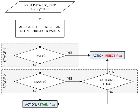
Figure 1Schematic summary of the proposed data cleaning procedure. SevEr and ModEr indicate strong and weak evidence about the presence of a specific source of systematic error, respectively.
In the second stage, flux data that inherited no SevEr statement are subject to an outlier detection procedure and only flux data that are both detected as outlier and inherited at least a ModEr statement are conclusively rejected. This implies that data points that inherited any number of ModEr statements but were not detected to be outliers, as well as outliers which showed no evidence of systematic errors, are retained in the dataset and can be used for any analysis or modelling purposes. In other words, only data points that provide strong evidence of error (either because of a SevEr or because of a ModEr and being identified as an outlier) are rejected, while peculiar data points, which would look suspicious to the visual inspection and are possibly identified as outliers, but only inherited NoEr statements, are retained.
The following section details the set of tests used in the proposed data-cleaning procedure and summarized in Table 1. Depending on their specification, tests are applied to individual high-frequency raw time series, pairs of variables, their statistics over the flux averaging interval, or even derived variables. For example, instrumental problems (see Sect. 2.2.1) are typically searched for on a per-variable basis, while stationarity conditions (see Sect. 2.2.3) are assessed by looking at the covariance between two variables. The test result is then inherited by all fluxes, to which the variable or variable pair is relevant. As an example, sensible heat flux H inherits the test results assigned to (at least) vertical wind speed w, sonic temperature Ts and the pair w∕Ts.
Foken and Wichura (1996)Mahrt (1998)Table 1Sources of systematic error, test statistics and adopted threshold values to define NoEr, ModEr and SevEr statements. Details on how the threshold values have been set are provided in Sect. 2.2.

The proposed data cleaning procedure is implemented in the RFlux R package (Vitale et al., 2019b) and is publicly available via the GitHub repository. The procedure has been designed and optimized for CO2∕H2O and energy EC fluxes over natural ecosystems based on current knowledge. However in different conditions (gas species, ecosystem, instrumentation, etc.), new tests and further optimization of the ones proposed here are possibly needed. As mentioned above, the data cleaning procedure is designed to naturally accommodate any number of tests that generate a statistic that can be compared against threshold values.
2.2 Detection of sources of systematic error affecting EC datasets
The possible sources of systematic errors are divided and analysed into three categories: (1) instrumental issues, (2) poorly developed turbulence regimes and (3) non-stationary conditions.
2.2.1 Detection of instrumental issues
Modern EC instruments can detect and report malfunctions occurring during the measurement process via diagnostic variables. However, there are situations where a measurement is affected by an error but it is still valid from the instrument's perspective, and for this reason it is not flagged by the instrument diagnostics. As an example, a physical quantity may have variations that are too small to detect, given the settings or the specifications of the instrument. This is the case of a time series of temperature that varies very little during a calm, stable night; the measurements may be affected by a low-resolution problem, where the quantization of the measurement due to the intrinsic resolution of the instrument becomes evident and leads to a reduced variability of the underlying signal. In this case, from the measurement perspective, there is nothing wrong with the measured quantity and diagnostics would not indicate any issues. In addition, with some instruments, especially older models, or often when collecting data in analogue format, diagnostic information is simply not available (Fratini et al., 2018). It is therefore useful to devise tests to detect instrument-related situations that are likely to generate systematic errors in resulting fluxes. In the following, we describe a series of routines to identify the most frequent errors caused by instrumental problems detectable on the raw, high-frequency time series (most of which were already discussed in Vickers and Mahrt, 1997, hereafter VM97).
Detection of unreliable records caused by system malfunction and disturbances
EC fluxes are calculated starting from the covariance between the vertical wind speed, w, and the scalar of interest computed over a specified averaging interval, typically 30 or 60 min. For the calculated covariance to be representative of the entire interval, the actual number of available raw data records should be close enough to the expected number (e.g. 18 000 records for fluxes over 30 min from raw data sampled at 10 Hz). If the number of available records is too small, the corresponding flux estimate may be significantly biased.
Data records can be unavailable for covariance computation for a variety of reasons. First, records may simply be missing because of problems during data acquisition. In addition, specific values may be eliminated if
-
instrumental diagnostics flag a problem with the measurement system;
-
individual high-frequency data points are outside their physically plausible range or are identified as spikes (in this work we used the despiking algorithm proposed by VM97);
-
data were recorded during periods when the wind was blowing from directions known to significantly affect the turbulent flow reaching the sonic anemometer sampling volume, e.g. due to the interference of the anemometer structure itself (C-clamp models) or to the presence of other obstacles;
-
the angle-of-attack of individual wind measurements is beyond the calibration range specified by the sonic anemometer manufacturer.
Note that the criteria above may apply to single variables, groups of variables (e.g. anemometric variables) or entire records. Although covariances can also be computed on time series with gaps, some of the procedures involved in the typical data processing do require continuous time series (e.g. the fast Fourier transform to compute power spectra and cospectra, or the stationarity tests that compute statistics on sub-periods as short as 50 s; Mahrt, 1998). The performance of such procedures may depend on the technique used to impute missing data (i.e. fill the gaps). It is therefore useful to establish criteria for the appropriate use of imputation procedures.
Typically, gaps in raw time series are filled using linear interpolation. While this algorithm provides obvious computational and implementation advantages, it should be noted that it only performs satisfactorily when the time series is dominated by low-frequency components, while it can introduce biases in time series characterized by significant high-frequency components, as is the case with EC data. Its application should thus be limited to very short gaps. The pattern of missing data plays a role too: when gaps occur simultaneously across all variables, linear interpolation can lead to biases in resulting covariances even for short gaps. Such biases are linearly proportional to the amount of missing data and relatively larger for smaller fluxes. These considerations also apply to other interpolation methods such as splines and the last-observation-carried-forward method.
With this in mind, by evaluating the fraction of missing records (FMR) and the longest gap duration (LGD) in time series involved in the covariance estimation, we suggest the following classification criteria:
-
SevEr if FMR >15 % or LGD >180 s,
-
ModEr if 5 % < FMR ≤ 15 % or 90 s < LGD ≤ 180 s,
-
NoEr if FMR ≤ 5 % and LGD ≤ 90 s.
Detection of low-signal-resolution problems
High-frequency EC data can be affected by low-signal-resolution problems (see VM97 for a detailed description). Resolution problems are mainly caused by a limited digitalization of the signal during data acquisition, when signal fluctuations approach the resolution of the instruments. This kind of problem causes a step ladder in the distribution of sampled data, and time series are characterized by the presence of repeated contiguous values. Instrumental faults can lead to a time series that remains fixed at a constant value for a period of time (dropout), analogously introducing artificial repeated values, though with a very different pattern of repetition. Repeated values are always to be considered an artefact since even in the (unlikely) event of a signal maintaining a constant value for an extended period of time, its measured values would still vary on account of the random error. In this particular scenario, contiguous repeated values would not actually lead to a bias in the flux estimate, because neglecting the presence of random error (as defined in the introductory section) does not affect covariance estimates. Instead when repeated values do not reflect the true dynamic of the underlying signal, they can lead to a significant bias in flux estimates. To disentangle these two situations, we evaluate the discrepancy between the w-scalar cross-correlation functions (CCFs) of the original time series and of the time series after removal of repeated values. If the discrepancy is negligible then the effect of repeated values on the covariance estimate is considered irrelevant. This could occur in the case of a small number of repeated data or if their values are still representative of the underlying signal dynamic. Conversely, when a significant discrepancy is found, the covariance estimate is considered biased. To evaluate the significance of such a discrepancy, we propose using the coefficient of determination (R2) of the linear regression through the origin of the CCFs estimated at short lags (±25 steps). The criteria used to assign a statement are as follows:
-
SevEr if R2<0.990,
-
ModEr if ,
-
NoEr if R2>0.995.
Detection of aberrant structural changes in time series dynamics
EC time series can be subject to regime changes such as sudden shifts in the mean and/or in the variance. In some circumstances, those are imputable to natural causes as in cases of intermittent turbulence (Sandborn, 1959) and wind pattern change over a heterogeneous or anisotropic footprint. In other cases, such changes are artefacts generated by instrumental malfunctions. Aberrant structural changes in mean and variance due to either environmental causes or measurement artefacts have similar effects on time series dynamics (which makes them difficult to disentangle) and lead to violation of the assumption of stationarity underlying the EC method. They should therefore be treated as sources of systematic errors. Here we propose three new tests to identify such situations, whose rejection rules are based on objective criteria but which, notably, do not discern natural changes from measurement artefacts.
The first test takes into consideration the homogeneity of the distribution of fluctuations (, where is the mean level estimated according to the averaging rule adopted in the covariance calculation, e.g. block average or linear detrending) and consists of evaluating the percentage of data in the tails with respect to the bounds imposed by Chebyshev's inequality theorem. Irrespective of the PDF generating the data, Chebyshev's inequality provides an upper bound to the probability that absolute deviations of a random variable from its mean will exceed a given threshold value. As an example, it imposes that a minimum of 75 % of values must lie within 2 standard deviations of the mean and 89 % within 3 standard deviations. When the inequality is violated, it is a symptom of data inhomogeneity due to structural changes in time series dynamics (e.g. abrupt change in the mean level and sudden upward or downward trend which may introduce significant bias in the estimation of the mean values and, consequently, of the covariances). In the following we indicate the test statistic related to the homogeneity of the distribution of fluctuations as HFB, where the subscript B indicates the sigma-rule adopted to define the boundary region (e.g. ±5σ).
The second test makes use of the same rule, but it evaluates the homogeneity of the distribution of first-order differenced data, (the corresponding statistic is denoted as HDB). Besides highlighting other useful properties, differencing a variable eliminates any trends present in it, whether deterministic (e.g. linear) or stochastic (Box et al., 2015), and the resulting time series is always stationary. Differencing acts as a signal filtering procedure and the transformed data can better highlight the characteristics of the measurement error process whose variance, under second-order stationary conditions, should be constant over time. Therefore, when the inequality is violated, it is a symptom of data inhomogeneity mainly due to changes in variance (heteroscedasticity). Based on the upper bounds imposed by Chebyshev's inequality for 5σ and 10σ, the first two tests are summarized in the following rules:
-
SevEr, if HF5>4 %, HD5>4 %, HF10>1 % or HD10>1 % (i.e. more than 4 % of fluctuations or differenced values are beyond the ±5σ limits or more than 1 % of them are beyond the ±10σ limits);
-
ModEr, if 2 % < HF5≤4 %, 2 % < HD5≤4 %, 0.5 % < HF10≤1 % or 0.5 % < HD10≤1 % (i.e. more than 2 % of fluctuations or differenced values are beyond the ±5σ limits or more than 0.5 % of them are beyond the ±10σ limits);
-
NoEr, if HF5≤2 %, HD5≤2 %, HF10≤0.5 % and HD10≤0.5 % (i.e. fewer than 2 % of both fluctuations and differences are beyond the ±5σ limits and fewer than 0.5 % of them are beyond the ±10σ limits).
As a robust estimate of σ, we used the Rousseeuw and Croux (1993) Qn estimator corresponding approximately to the first quartile of the sorted pairwise absolute differences. Compared to other robust scale estimators – such as the median absolute deviation about the median (MAD) and the interquartile distance (IQD) – it is a location-free estimator; i.e. it does not implicitly rely on a symmetric noise distribution. Similar to MAD, its breakdown point is 50 %; i.e. it becomes biased when 50 % or more of the data are large outliers. However, its efficiency is larger, especially when identical measurements occur, e.g. due to low-signal-resolution problems.
The third test consists of evaluating the kurtosis index on the differenced data Δyt (hereafter denoted KID test). The kurtosis index is defined by the standardized fourth moment of the variable about the mean. Because variations about the mean are raised to the power of 4, the kurtosis index is sensitive to tail values of the distribution and can therefore be used to characterize them (Westfall, 2014). Since the tails of a distribution represent events outside the “normal” range, a higher kurtosis means that more of the variance is contributed by infrequent extreme observations (i.e. anomalies) as opposed to frequent, modestly sized deviations. The sensitivity to tail values and the application to differentiated values make the KID a very useful tool to detect a range of instrumental problems, which include abnormal changes in mean, variance, but also the presence of undetected residual spikes and drop-out events (in these situations differenced time series will show a spike in correspondence of each change point).
To eliminate the sensitivity of the KID to the presence of repeated values (which become zeros in the differenced variable), such values were not included in KID estimation. Bearing in mind that the kurtosis index for a Gaussian and a Laplace PDF is equal to 3 and 6, respectively, we choose reasonably large threshold values to make sure we select only time series characterized by heavy-tailed distribution as is the case of data contaminated by extreme events representative of the aforementioned problems. Namely, we suggest that the following criteria be applied:
-
SevEr if KID > 50,
-
ModEr if 30 < KID ≤ 50,
-
NoEr if KID ≤ 30.
2.2.2 Detection of poorly developed turbulence regimes
One of the assumptions underlying the EC method is the occurrence of well-developed turbulence conditions. A widely used test to assess the quality of the turbulence regime is the integral turbulence characteristics (ITC) test proposed by Foken and Wichura (1996, hereafter FW96). Based on the flux-variance similarity theory, the test consists of quantifying the relative change of the ratio between the standard deviation of a turbulent parameter and its corresponding turbulent flux (the “integral characteristic”) with respect to the same ratio estimated by a suitable parameterization. The ITC can be calculated for each wind component and any scalar (temperature and gas concentration), but for the purpose of data cleaning, the ITC for vertical wind speed is used (see Foken et al., 2012b). This is defined as
where σw is the standard deviation of the vertical wind speed w, u* the friction velocity and the parameterization as a function of the dynamic measurement height (z−d) and the Obukhov length L, with c1 and c2 being parameters varying with atmospheric stability conditions, as tabulated in Foken et al. (2012b, Tables 4.2 and 4.3).
The criteria adopted to assign SevEr, ModEr and NoEr statements are based on threshold values proposed by Mauder and Foken (2004, Table 16). In particular,
-
SevEr if ITC > 100,
-
ModEr if 30 < ITC ≤ 100,
-
NoEr if ITC ≤ 30.
2.2.3 Detection of non-stationary conditions
The working equation of turbulent fluxes as the (appropriately scaled) w-scalar covariance is based on a simplification of the mass conservation equation (see e.g. Foken et al., 2012a). One of the assumptions behind such simplification is that of stationary conditions, which are however not always fulfilled during the measurement period. Diurnal trends, changes in meteorological conditions (e.g. passage of clouds), boundary layer transitions, large-scale variability and changes in footprint areas are only some example of sources generating non-stationary conditions. In the presence of non-stationarity, flux estimates are biased. The magnitude and sign of the systematic error depend on the nature of the non-stationarity, on the proportion of total variability explained by trend components and on the way (deterministic or stochastic) independent trend components interact with each other.
To avoid biases, a possible approach is to preliminarily remove the source of non-stationarity before calculating covariances. This way, the amount of data rejected for non-stationary conditions can be limited. To this end, procedures based on linear detrending or running mean filtering are often used during the raw data processing stage. However, their application can be ineffective, for example when linear detrending is used on nonlinear trends (see the Supplement, Sect. S2) and even risk introducing further biases when data are truly stationary or when non-stationarity is of more complex nature (see Rannik and Vesala, 1999; Donateo et al., 2017, for a comparison of detrending methods). For this reason, an alternative approach is to remove periods identified as non-stationary.
A few tests have been proposed for EC data, of which we discuss two popular ones. A widely used statistic is based on a test introduced by FW96, based on the comparison between the covariance computed over the flux averaging period T (30 or 60 min) and the average of covariances computed on shorter intervals I (in the original proposal, six periods of 5 min each if T is 30 min). The test statistic is defined as
where is the mean covariance obtained by averaging covariances computed on I intervals, and is the covariance computed over the period T. According to the authors' suggestion, stationary conditions are met when SFW96≤30 %.
A major problem with Eq. (4) is that when the covariance at the denominator is close to zero, the test statistic will approach infinity, making the ratio unstable. As a consequence the FW96 test is disproportionately sensitive to fluxes of small magnitude (see also Pilegaard et al., 2011).
An alternative test was proposed by Mahrt (1998, hereafter M98). This test measures non-stationarity by comparing the effects of coherent behaviour with the inherent random variability in the turbulent signals. As with FW96, the time series is divided into I non-overlapping intervals of 5 min; in this case however each interval is also divided into J=6 non-overlapping subintervals of 50 s. The test statistic is defined as
where σB is a measure of the variability of the covariance between different intervals calculated as
and σW is a measure of the average variability within each interval i and is given by
with denoting the covariance computed over the flux averaging period, the covariance relative to the ith 5 min interval and the covariance relative to the jth 50 s subinterval within the ith interval. Mahrt (1998) recommended rejecting flux data when SM98>2, without excluding the possibility to increase the threshold value, bearing in mind that a high threshold value could be particularly risky for high towers in situations with strong convection.
With respect to the FW96 test, the non-stationarity ratio by M98 is always well-behaved with the denominator strictly positive (average of standard deviations). For this reason, the test proposed by M98 was selected for this work. Based on a performance evaluation described later in this paper (see Sect. 3), we suggest the following flagging criteria:
-
SevEr if SM98>3,
-
ModEr if ,
-
NoEr if SM98≤2.
2.3 Outlier detection for half-hourly EC flux time series
As described in Sect. 2.1, the second step in the data cleaning procedure consists of detecting outlying fluxes and removing them if they inherited at least one ModEr statement. Outlying fluxes can be caused by a variety of sources involving instrument issues and natural causes (e.g. non-stationary conditions as often occur during post-dawn transition from a stable to a growing/convective boundary layer).
The outlier detection proceeds as follows: first, a signal extraction is performed, to obtain an estimate of the true signal; the residual term is estimated as and a PDF is built for it; outlying observations are then defined as those fluxes for which the residual falls in the tails of the distribution, according to pre-specified threshold values. In the general case, extreme values of model residuals can occur for three reasons: (i) the model is misspecified and the residual is due to a wrong estimate for , (ii) the residual is due to the presence of a non-negligible systematic error (i.e. in Eq. 2) or (iii) the residual is indeed a tail instance on the PDF of et.
Condition (i) can be assessed by examining the degree of serial correlation in the residual time series. When a model is correctly specified, residuals should not show any serial correlation structure and resemble a white noise process. Distinguishing between conditions (ii) and (iii) is not trivial and would require an in-depth analysis of the causes generating the anomalies. We propose considering the presence of at least a ModEr statement as a symptom of condition (ii) and thus rejecting flux data identified as outliers and flagged with at least a ModEr statement. Otherwise, if all tests return NoEr statements, the outlying data are retained irrespective of the magnitude of the anomaly. Details about the modelling framework and how to take into account the heteroscedastic behaviour of the residual component are provided in the following.
2.3.1 Signal extraction
For the purpose of signal extraction, we considered the following multiplicative model:
where Dt represents the diurnal cycle, LRTt represents the long-run (e.g. annual) trend, SRTt is the short-run (e.g. the intra-day) temporal dynamics term and It is the irregular or residual component, considered as an estimate of et in Eq. (1). The choice of a multiplicative model is preferred when the amplitude of the cyclic component is proportional to the level (i.e. the long-run trend) of the time series (see Hyndman and Athanasopoulos, 2018, chap. 6). Such a dynamic is typical of those ecosystems characterized by diurnal cycles of fluxes which are more pronounced during growing than during dormant seasons.
The estimation of each component in Eq. (8) can be performed in a variety of ways. In this work we used the STL (seasonal-trend decomposition based on LOESS – locally estimated scatterplot smoothing) algorithm developed by Cleveland et al. (1990) and implemented in the stlplus R software package (Hafen, 2010, 2019). We choose the STL algorithm because of its flexibility and computational efficiency in modelling both the cyclic and the trend components of any functional forms and because of its ability to handle missing values.
The main steps of the STL algorithm are as follows. To separate out the diurnal cycle component, STL fits a smoothing curve to each sub-series that consists of the points in the same phase of the cycles in the time series (i.e. all points at the same half hour of day, for diurnal cycles). After removing the diurnal cycle, it fits another smoothing curve to all the points consecutively to get the trend components. This step can be executed iteratively in the presence of outliers. In particular, the STL algorithm deals with outliers by down-weighting them and iterating the procedure of diurnal cycle and trend component estimation. As the diurnal cycle and trend are smoothed, outliers tend to aggregate in the irregular component. The span parameters of the loess functions used for the extraction of the Dt and LRTT were set equal to 7 d, while those for SRTt were set equal to seven half-hour periods. The degree of locally fitted polynomials in Dt and LRTt extraction was imposed to be linear, while that in SRTt extraction was imposed to be constant. The number of iterations involved was set equal to 20.
The ability of the model to adequately describe the dynamics of the time series under investigation is determined by analysing the statistical properties of the residual time series. As mentioned above, a properly fitted model must produce residuals that are approximately uncorrelated in time. Any pattern in residuals, in fact, indicates the fitted model is misspecified and, consequently, some kind of bias in fitted values is introduced. To this end, spectral properties of the incomplete residuals are assessed through the Lomb–Scargle (LS) periodogram (Lomb, 1976; Scargle, 1982). This method is particularly suited to detect periodic components in time series that are unequally sampled as a consequence of the presence of missing data at this stage of the data cleaning procedure.
2.3.2 Outlying flux data
Previous studies focusing on flux random uncertainty quantification have evidenced a heteroscedastic behaviour of the random error (see Richardson et al., 2012, and references therein). Furthermore, it has been demonstrated that the random error distribution can be better approximated by a Laplace than by a Gaussian distribution (Vitale et al., 2019a). To take into account these features, residuals are first grouped into 10 clusters of equal size (defined by percentiles) based on the estimated flux values. Then, for each of the 10 clusters, the outlier detection is performed assuming a Laplace distribution and taking into account the (1−α) % confidence interval with α=0.01 given by μ±log (α)σ, where μ (location) is estimated by the median, and the scale parameter, σ, is estimated through the Qn estimator by Rousseeuw and Croux (1993) for the same reasons introduced in Sect. 2.2.1.
It is important to note here that a significant limitation of the proposed outlier detection method is the inability to detect systematic errors whose sources act constantly across a flux time series, for long periods of time. As an example, a miscalibration of the instruments that persists for days would most likely not be identified as outlying fluxes by the proposed outlier detection procedure. Such sources of systematic errors should be prevented via appropriate QA actions or, at least, specific QC tests should be devised, able to mark those time series with SevEr statements.
2.4 Monte Carlo simulations
This work has made extensive use of Monte Carlo experiments that make use of simulated time series mimicking raw EC datasets. The main purpose of the simulations is to create pairs of reference time series with known covariance structure that, after being contaminated with a specific source of systematic error, allow a quantitative and objective evaluation of (i) the bias effect the source of systematic error has and (ii) the ability of proposed tests to correctly detect it. We note that, for these purposes, it is not strictly required to simulate medium- or long-term time series with realistic joint probability distributions from which to generate half-hourly fluxes with typical diurnal and seasonal cycles. In fact, it is reasonable to assume that QC tests exhibiting poor performances on simulated data have little chance of success when applied to observed time series which can exhibit more complex structures of the underlying signal and of the (random) measurement error process, and which can be contaminated by the simultaneous occurrence of several sources of systematic errors.
Based on the main properties of EC time series (summarized in Sect. S1), synthetic time series were created from two first-order autoregressive processes (hereafter denoted AR; see Sect. S2 for an overview of their stochastic properties) representative of the vertical wind speed and of the atmospheric scalar. The procedure adopted to ensure that simulated AR processes have a pre-fixed correlation structure is described in Sect. S3. All simulations were executed in the R programming environment (R Development Core Team, 2019).
Several scenarios have been considered to simulate stationary time series with different degrees of temporal dependence and with pre-fixed correlation structures in order to simulate fluxes of different magnitude. All simulated time series have 18 000 data points as in EC raw high-frequency time series sampled at 10 Hz and collected in 30 min files. Once simulated, time series were then contaminated with specific sources of systematic error, the details of which will be provided in Sect. 3.
2.5 Eddy covariance datasets and flux calculations
In this study, data from 10 EC sites that are part of the ICOS network (ICOS RI, 2019) were used: BE-Lon (Lonzee, Belgium, cropland; Moureaux et al., 2006), CH-Dav (Davos, Switzerland, evergreen needleleaf forest; Zielis et al., 2014), DE-HoH (Hohes Holz, Germany, alluvial forest; Wollschläger et al., 2017), DE-RuS (Selhausen Juelich, Germany, cropland; Schmidt et al., 2012), FI-Hyy (Hyytiälä, Finland, evergreen needleleaf forest; Suni et al., 2003), FI-Sii (Siikaneva, Finland, wet grassland; Haapanala et al., 2006), FR-Fon (Fontainebleau, France, deciduous broadleaf forest; Delpierre et al., 2015), IT-SR2 (San Rossore 2, Italy, evergreen needleleaf forest; Matteucci et al., 2015), SE-Htm (Hyltemossa, Sweden, evergreen needleleaf forest; van Meeningen et al., 2017) and SE-Nor (Norunda, Sweden, boreal forest; Lagergren et al., 2005).
The lack of knowledge of the reference flux value and of the contributions of systematic and random error drastically limits the use of field data in test performance evaluation. However, field data are crucial to an evaluation of the impact the proposed data cleaning procedure and, in particular, to understand which is the main source of systematic error affecting flux variables. Although the performance evaluation of the proposed tests is mainly carried out via Monte Carlo simulations, a selection of raw data were also used to provide representative examples of test application.
The turbulent fluxes of CO2 (FC, µmol CO2 m−2 s−1), sensible heat (H, W m−2) and latent heat (LE, W m−2) were calculated from the covariances between the respective scalar and the vertical wind speed (w, m s−1) following the standard EC calculation method (see e.g. Sabbatini et al., 2018). The EddyPro® software (LI-COR Biosciences, 2019) was used to this aim, employing the double coordinate rotations for tilt correction, 30 min block averaging, the maximum cross-covariance method for time lag determination and the in situ spectral corrections proposed by Fratini et al. (2012).
The net ecosystem exchange of CO2 (NEE, µmol CO2 m−2 s−1) was estimated by integrating FC with the concurrent storage flux (SC, µmol CO2 m−2 s−1), calculated by means of the single profile approach (Aubinet et al., 2001). Although more consistent estimates can be achieved by means of multiple profile sampling (Nicolini et al., 2018), it is important to note that the choice of the storage estimation method does not drastically affect the results of the proposed data cleaning procedure since the test statistics are mainly based on turbulent raw data.
3.1 Performance evaluation of QC tests
3.1.1 Low-signal-resolution (LSR) test
A simulation study was carried out with the twofold aim of quantifying the bias caused by low-signal-resolution problems and evaluating the performance of the LSR test described in Sect. 2.2.1.
To this end, error-free AR processes of length n = 18 000 were first simulated and subsequently contaminated with artificially generated errors. The correlation between time series has been set to 0.1, simulating medium to low fluxes, while the autoregressive coefficient (ϕ) was allowed to take on a value in the set [0.90, 0.95, 0.99] to represent different degrees of serial dependence (i.e. autocorrelation) as observed in EC data (Sect. S1). Low-resolution problems were simulated (i) by rounding the simulated values from 2 to 0 digits and (ii) by sampling at random an increasing percentage of data (15 %, 30 %, 45 %, 60 % and 75 % of the sample size) and then replacing it via the last-observation-carried-forward (LOCF) imputation technique. This allows the creation of a typical ramp structure as is commonly encountered in raw, high-frequency time series.
In summary, the following six macro-scenarios, , were considered:
-
AR processes with ϕ=0.90 contaminated by rounding the values from 2 to 0 digits;
-
AR processes with ϕ=0.95 contaminated by rounding the values from 2 to 0 digits;
-
AR processes with ϕ=0.99 contaminated by rounding the values from 2 to 0 digits;
-
AR processes with ϕ=0.90 contaminated by replacing 15 %, 30 %, 45 %, 60 % and 75 % of their values via LOCF;
-
AR processes with ϕ=0.95 contaminated by replacing 15 %, 30 %, 45 %, 60 % and 75 % of their values via LOCF;
-
AR processes with ϕ=0.99 contaminated by replacing 15 %, 30 %, 45 %, 60 % and 75 % of their values via LOCF.
Each of the six macro-scenarios was run 999 times to obtain robust statistics. Three realizations of corrupted AR processes are depicted in Fig. 2.
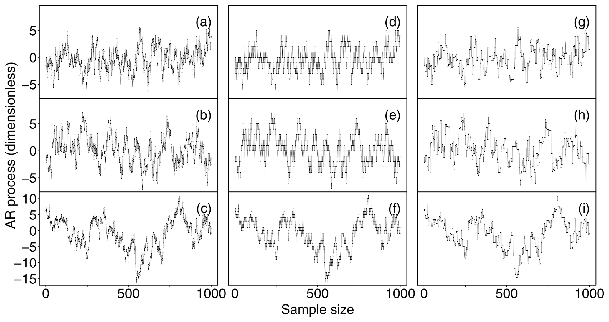
Figure 2Three realizations of AR processes of length 1000 with ϕ=0.9 (a), ϕ=0.95 (b) and ϕ=0.99 (c), affected by low-resolution problems simulated by discretizing the original variable (d–f) and by replacing 60 % of original data via the last-observation-carried-forward (LOCF) technique (g–i).
Bias affecting correlation estimates was quantified as the difference in absolute percentage between the correlation estimated on error-free (ρEF) and on contaminated (ρC) data. Results for each scenario are shown in Fig. 3. When low-resolution problems were simulated by rounding values (), the bias was less than 2 %. Similar results were reported by VM97 and more recently by Foken et al. (2019). Conversely, when low-resolution problems were simulated by replacing values via LOCF, a significant bias was introduced in correlation estimates, whose amount depends not only on the number of contaminated data, but also on the degree of serial dependence. As expected, with the percentage of data affected by error being equal, the lower the degree of serial correlation, the higher the amount of bias. In , when the AR processes were simulated with ϕ=0.90, a bias greater than 5 % was observed as soon as more than 30 % of data were contaminated by error. Conversely, when ϕ=0.99 as in , the bias was less than 5 %, even when 75 % of data were contaminated by error. This is because when a series has strong autocorrelation, the following values are expected to be close to the current value, and therefore replacing them with the current value does not change the time dynamic significantly and as a consequence the correlation estimate remains unbiased.
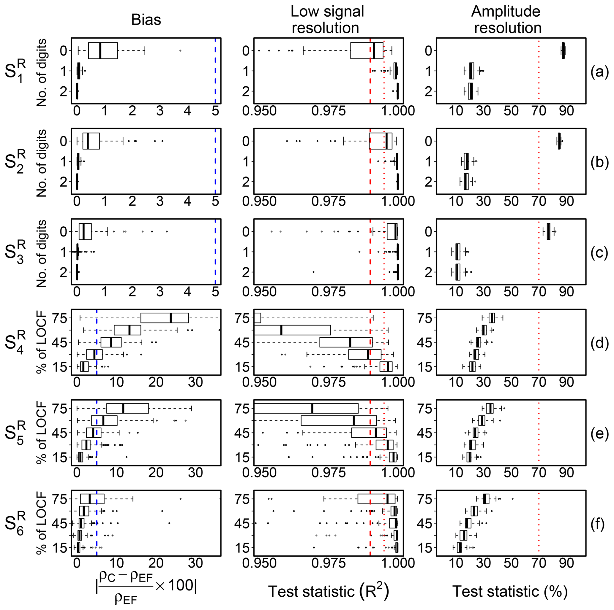
Figure 3Bias effect of low-signal-resolution problems and test performance evaluation in the scenarios (a–f, respectively) described in Sect. 3.1.1. The left panels show the difference in percentage between correlation estimated on error-free time series (ρEF) and on data contaminated (ρC) by low-resolution problems (dashed blue line indicates 5 % bias). The middle panels show the distribution of the test statistic (R2) for the low-signal-resolution (LSR) test; dashed red lines indicate the threshold values at 0.99 and 0.995 adopted for defining the SevEr and ModEr statements, respectively. The right panels show the distribution of the amplitude resolution test statistic by VM97; dashed red lines indicate the threshold value at 70 % as recommended by the authors for assigning a hard flag to data. In the (a) and (d) scenarios, the AR processes were simulated with ϕ=0.90, in (b) and (e) with ϕ=0.95, and in (c) and (f) with ϕ=0.99.
The ability of the LSR test to disentangle among these situations can be appreciated by looking at the distribution of the R2 values in the six scenarios as shown in Fig. 3 (middle panels). To aid in comparison we also added the results of the amplitude resolution test by VM97 (right panels of Fig. 3). Considering threshold values at 0.99 and 0.995 to identify SevEr and ModEr statements, the LSR test showed good performance with false-positive and false-negative rates much lower than the amplitude resolution test. For the latter, low-resolution problems were identified only for scenarios and limited to cases when the number of digits is reduced to zero. The amount of bias in such cases was however negligible. Conversely, the sensitivity of the LSR test was such that the higher the bias affecting correlation estimates the lower the R2 values, irrespective of the low-resolution simulation method.
We applied both LSR and amplitude resolution testing procedures to the selected field datasets described in Sect. 2.5 (results are reported in Sect. S4). For LE and NEE, similar amounts of data were flagged by the two tests. Conversely, for the sensible heat flux the LSR test flagged much fewer data than the amplitude resolution test. In particular, for five sites the percentage of H data hard-flagged by the amplitude resolution test exceeded 40 % with a maximum of 68.3 % at SE-Htm. The hard flag was often assigned by the amplitude resolution test to the sonic temperature time series during periods of low variability, which led to the typical step ladder in the data. However, in most of these cases, that does not necessarily imply biased covariance estimates.
To aid in comparison, some illustrative examples are shown in Fig. 4. Panel (a) shows a sonic temperature time series for which both tests provide negligible evidence of error. Notice that in this case, the R2 is close to unity although 19.8 % of data were constituted by repeated values. The case shown in panel (b) is representative of contrasting results: the amplitude resolution test assigned a hard flag, while the LSR test returned a NoEr statement. By visual inspection, it would seem that despite the step-ladder appearance in the data, the time series dynamic is mostly preserved. In these occurrences, bias affecting covariance estimates is typically negligible, as demonstrated by the fact that the CCFs estimated with original data and after removal of repeated values overlap almost perfectly. The cases depicted in panels (c) and (d) are representative of situations of strong resolution issues leading to diverging CCFs and significant biases. The LSR test successfully detects both problems, while the amplitude resolution test fails to flag case (c).
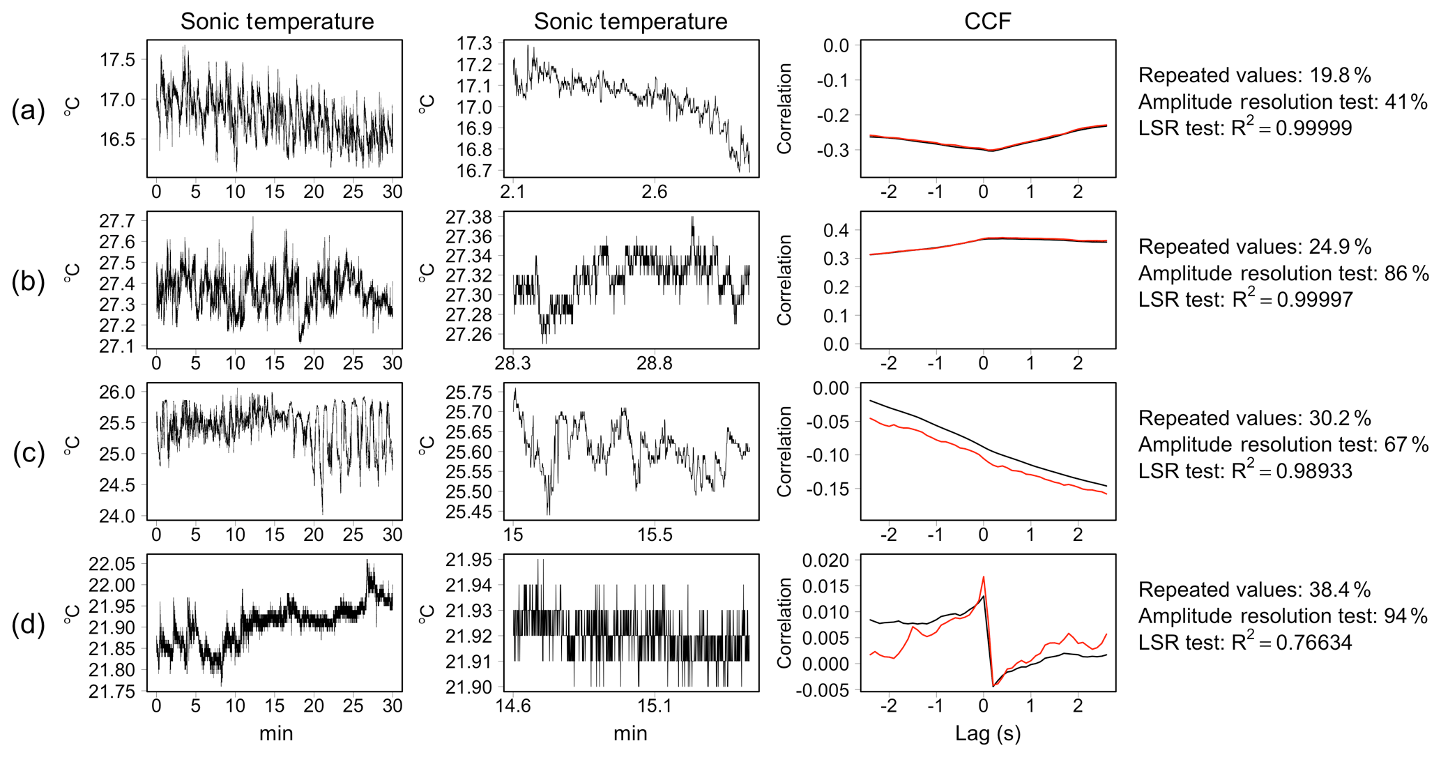
Figure 4Comparison of low-signal-resolution (LSR) test and amplitude resolution test by VM97 on observed data collected at the SE-Nor site. Sonic temperature time series collected in 30 min (left panels) and in a shorter temporal window of length equal to 1000 time steps (middle panels). The right panels show the cross-correlation function (CCF) between w-scalar time series with original data (black line) and after removal of repeated values (red line). The percentage of repeated consecutive values, the test statistics of the amplitude resolution and LSR tests are reported on the right-hand side.
3.1.2 Structural changes tests
The Monte Carlo experiment designed for the evaluation of the performance of the proposed structural changes tests described in Sect. 2.2.1 involved six scenarios, , where several synthetic AR processes (ϕ=0.99) of length n = 18 000 were contaminated by ).
-
a stochastic trend;
-
a deterministic linear trend;
-
an abrupt change in the mean level whose duration and shift were fixed at 3000 time steps and 3 times the interquartile distance (IQD) of the data, respectively;
-
multiplying a block of consecutive data of size 6000 (corresponding to 10 min in EC raw data sampled at 10 Hz) by a cosine function to mimic episodic burst events as often observed in real data;
-
introducing 0.5 % of spiky data generated by adding 2×IQD to the original data;
-
replacing 15 % of the data with the original values multiplied by 5, to simulate changes in variance.
Although these scenarios only cover a fraction of the problems encountered in real observations, the experiment aims at evaluating the test sensitivity in the presence of aberrant structural changes which, in most cases, can only be imputable to malfunction of the measurement system. Note that scenarios do not aim at simulating time series affected by structural changes. Rather, their purpose is to evaluate the propensity of the tests to produce false-positive errors.
An illustrative example of the simulated AR process mimicking sonic temperature time series contaminated by structural changes according to the scenarios is shown in Fig. 5. Each scenario was run 999 times. For each simulation, the statistics of the HF5, HD5 and KID tests were calculated. As a reference, we also applied the “discontinuity” and “kurtosis index” tests proposed by VM97 (while their “dropouts” and “skewness” tests resulted in insensitivity to the simulated scenarios and will therefore not be further discussed). Results are summarized in Fig. 6.
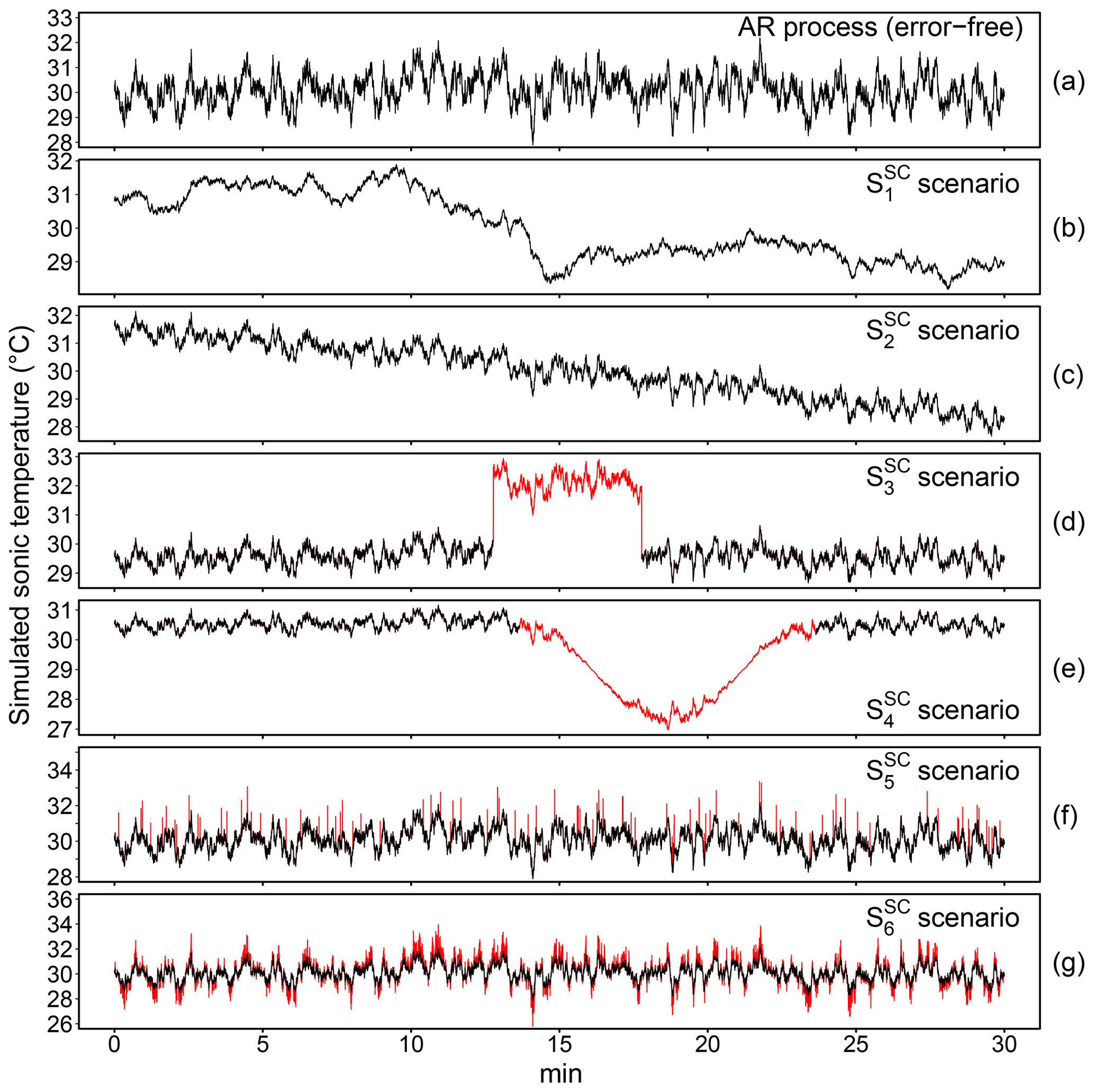
Figure 5Illustrative example of an autoregressive (AR) process (a) contaminated by a stochastic trend (b, scenario), by a deterministic linear trend (c, scenario) and by various structural changes (red lines) according to the scenarios described in Sect. 3.1.2 (d–g).

Figure 6Distribution of results for the structural change detection tests in the scenarios described in Sect. 3.1.2. Horizontal short and long dashed red lines indicate the threshold values adopted for defining SevEr and ModEr statements (hard and soft flag for VM97 tests), respectively.
We observe that all tests exhibited a low false-positive error rate (compare scenarios and ). The only exception was the VM97 test based on the Haar transform to detect discontinuities in the mean level (Fig. 6a), which instead showed poor performance when time series were contaminated by a stochastic trend component. The sudden shift in mean level simulated in the scenario was correctly identified by the KID test in most simulations (Fig. 6f). The Haar transform for detecting discontinuity in the mean level identified the simulated structural changes, but only in fewer than 50 % of cases in which the hard flag was assigned (Fig. 6a). Good performances were observed in the scenario for both the Haar transform for detecting discontinuity in mean (Fig. 6a) and the HF5 test (Fig. 6b). Structural changes caused by heteroscedastic behaviour simulated in the and scenarios were correctly detected by only KID (Fig. 6f) and HD5 tests (Fig. 6d), respectively. The kurtosis index (estimated on de-trended time series) was almost always lower than threshold values suggested by VM97 and therefore never detected any of the structural changes simulated in this Monte Carlo study (Fig. 6e).
The application of the testing procedures on actual EC time series has shown a higher sensitivity of the VM97 tests, compared to the newly proposed tests, with a tendency to assign hard flags even in cases in which no evidence of instrumental error was supported by visual inspection. Conversely, the proposed tests were more selective at identifying data affected by structural changes, although in some cases such structural changes were not necessarily imputable to instrument malfunction. In most of these occurrences, however, structural changes are indicative of non-stationary conditions, which as we know are another source of systematic error that introduces bias in covariance estimates (see Sect. 3.1.3). This is an example where two tests are not fully independent and could identify the same issue, which is why the ModEr statements are not combined. Illustrative examples of application of the testing procedures on raw data are shown in Fig. 7.
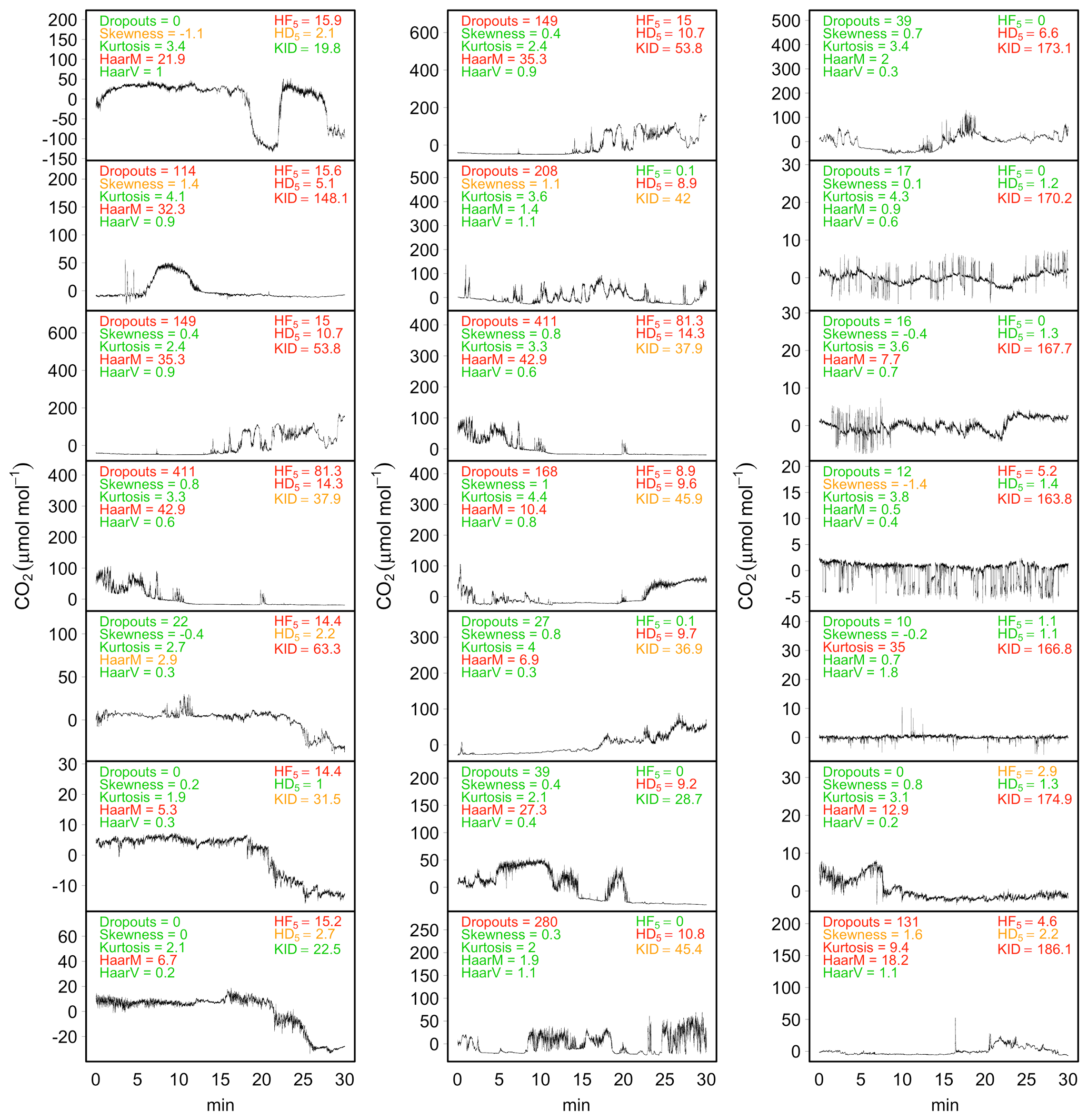
Figure 7Application of tests for structural change detection on a selection of CO2 time series (µmol mol−1, after mean removal) collected at the BE-Lon site. The statistics of dropouts, skewness, kurtosis, discontinuities in mean (HaarM) and variance (HaarV) tests as described by VM97 and the statistics of HF5, HD5 and KID tests described in Sect. 2.2.1 are reported at the top of each panel. For each test, green text indicates NoEr (no flag by VM97 tests), orange text indicates ModEr (soft flag) and red text indicates SevEr (hard flag).
3.1.3 Stationarity tests
We compared the performance of the stationary tests by FW96 and by M98 via Monte Carlo simulation making use of synthetic bivariate pairs of AR processes, xt as representative of vertical wind speed and yt as representative of scalar atmospheric concentrations, with t=1, …, n = 18 000, according to the following scenarios:
-
and simulating fluxes of low magnitude;
-
and simulating fluxes of high magnitude;
-
and simulating fluxes of low magnitude, but in the presence of time series with a high degree of serial correlation;
-
and simulating fluxes of high magnitude, but in the presence of time series with a high degree of serial correlation;
-
as in , where both xt and yt were contaminated by deterministic linear trend components;
-
as in , where both xt and yt were contaminated by deterministic linear trend components;
-
as in , where both xt and yt were contaminated by stochastic trend components;
-
as in , where both xt and yt were contaminated by stochastic trend components.
Notice that the scenarios simulate fluxes measured under stationary conditions (by definition, since ), while the remaining scenarios simulate fluxes measured under non-stationary conditions. Each scenario was run 999 times.
To mimic trend dynamics of magnitude similar to those observed in real cases, the slope of the deterministic linear trend function , was fixed equal to 0.0004 and 0.004 for xt and yt, respectively. In the case of time series of length n = 18 000, as in EC raw data sampled at 10 Hz in an average period of 30 min, a slope coefficient equal to 0.0004 (0.004) increases the mean level of 7.2 (72) units of the response variable, respectively (e.g. 7.2 m s−1 for vertical wind speed, 72 µmol mol−1 for CO2 concentrations, 72 K for sonic temperature).
Stochastic trend components were generated as , where ε is drawn from a normal distribution with a mean of 0 and standard deviation (s) equal to 0.025 and 0.25 for xt and yt, respectively. Consequently, the sum of such variables is normal with a mean of 0 and standard deviation . In the case of time series of length n = 18 000, as in EC raw data sampled at 10 Hz in an average period of 30 min, s equal to 0.025 (0.25) generates an ensemble of stochastic trajectories, responsible for non-stationary conditions, whose standard deviation at n = 18 000 is σ=3.35(33.5) units of the response variable (e.g. metres per second for vertical wind speed, micromoles per mole for CO2 concentrations, kelvin for sonic temperature).
Representative realizations of the simulated AR processes and their CCFs estimated on either single run and averaged over multiple runs (i.e. ensemble CCF) are illustrated in Fig. 8.
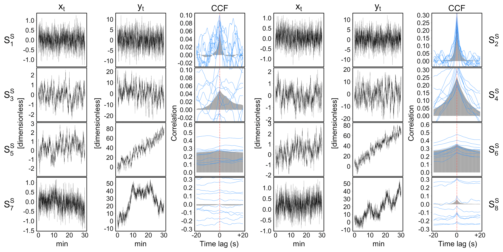
Figure 8Illustrative examples of simulated AR processes, xt and yt, and their cross-correlation function (CCF) in each of the eight scenarios, , described in Sect. 3.1.3 and designed to evaluate the performance of the stationarity tests. Grey areas represent the ensemble CCF averaged over multiple simulation runs. Blue lines represent the CCF estimated in 10 individual simulation runs.
Results of applying the FW96 and M98 stationarity tests for each of the eight scenarios considered are shown in Fig. 9. Test performances were evaluated through a statistical sensitivity analysis given by the percentage of correctly identified cases. The threshold values used to assign ModEr and SevEr statements were 30 % and 100 % for FW96 and 2 and 3 for M98, respectively.
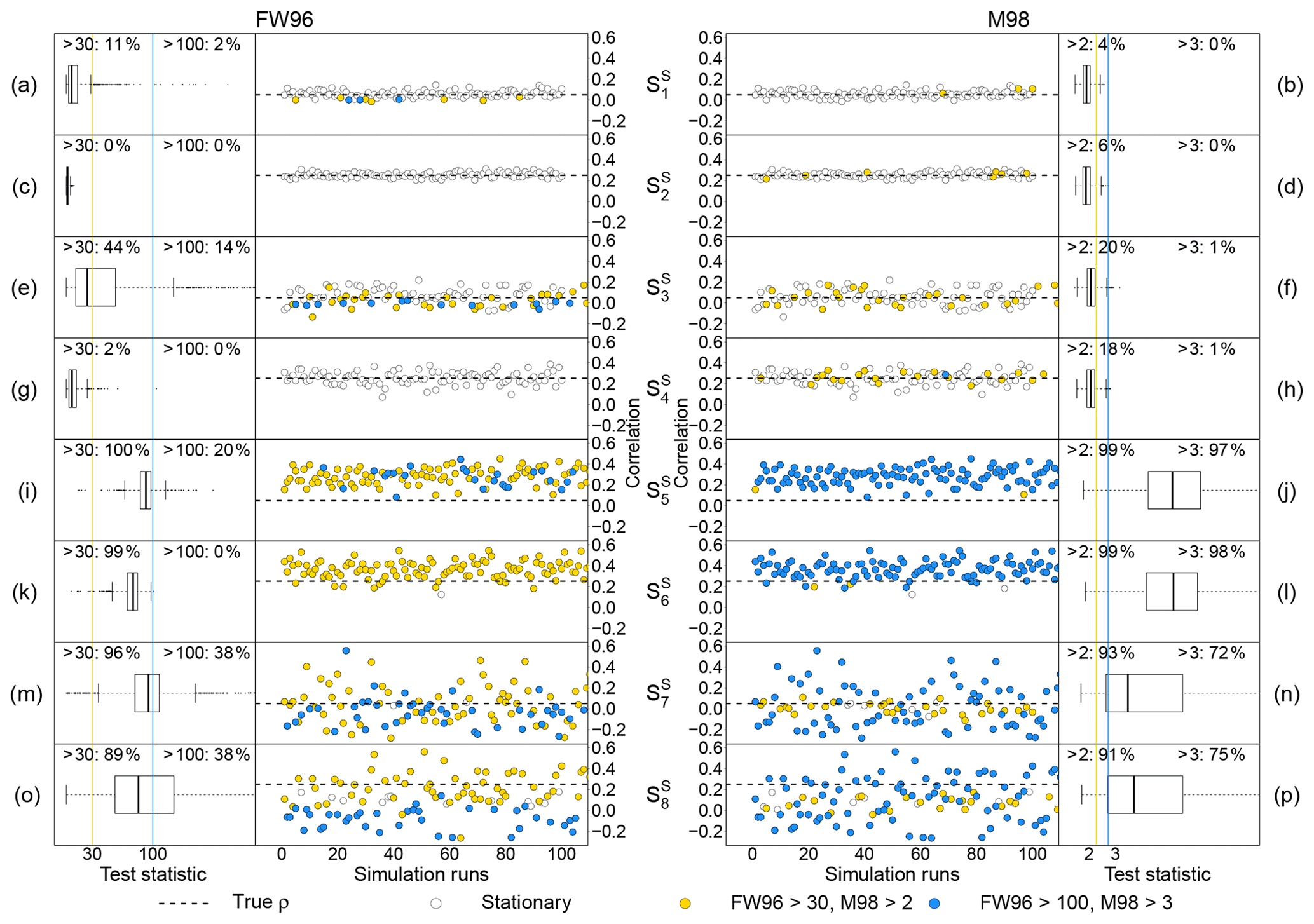
Figure 9Performance evaluation of the stationarity tests by Foken and Wichura (1996, FW96) and by Mahrt (1998, M98) in each of the simulated scenarios described in Sect. 3.1.3. Left and right panels show the distribution of the FW96 and M98 test statistics, respectively, in 999 simulation runs; percentage values are reported at the top of panels (a)–(p); yellow and blue vertical lines indicate threshold values (30 % and 100 % for FW96, 2 and 3 for M98; see Sect. 2.2.3 for more details). The middle panels show the distribution of the test statistic as a function of the correlation between variables in the first 100 simulation runs; yellow and blue points indicate simulations when the test statistic exceeds the corresponding threshold values; the horizontal dashed line indicates the pre-fixed true correlation, ρ, used in simulations.
In the and scenarios, where simulated time series are stationary and characterized by a lower degree of serial correlation, both tests exhibited good performances (Fig. 9a–d). The fraction of cases in which the statistics exceeded the threshold values that would, wrongly, lead to the rejection of data (i.e. 100 % for FW96 and 3 for M98) was less than 5 %, with a slightly better score for M98. In and (Fig. 9e–h), with stationary time series characterized by a higher degree of serial correlation, the performance of the FW96 test appeared discordant: unlike the excellent performance obtained in , in the test statistic was higher than 30 % in 44 % of cases and greater than 100 % in another 14 %. The cause of this low performance is related to the sensitivity of the FW96 test to cases in which its denominator (i.e. covariance over the entire period) approaches zero and thus tends to make the ratio diverge, independent of the numerator. The M98 test instead showed a lower sensitivity to low correlations among variables but a greater sensitivity to the degree of serial correlation. In both and , the percentage of data in which the test statistic was greater than 2 was in fact higher than 15 %. At the same time, however, in only 1 % of cases did the statistic exceed 3, the threshold value adopted to assign a SevEr statement. This result indicates that the use of 3 instead of 2 as a threshold value for the M98 test is preferable since it reduces the false-positive error rate.
In both and (Fig. 9i–l), the M98 test showed an excellent ability to detect non-stationarity caused by the presence of deterministic linear trend components: the statistic was higher than 3 in more than 95 % of cases. Conversely, for the FW96 test a similar performance would require the use of a 30 % threshold value. However, according to the recommendations of Foken et al. (2004), when the value of the statistics is between 30 % and 100 %, if well-developed turbulence conditions are satisfied, the data would not be rejected but classified as data of intermediate quality. In the presence of stochastic trend components as simulated in scenarios and (Fig. 9m–p), the M98 test performed better than the FW96 test. However, the false-negative error rate (i.e. data erroneously considered stationary) remained higher than 20 % when using 3 as a threshold value. In particular, only 72 % and 75 % in the and scenarios, respectively, received the status of data affected by SevEr.
The performance considerations described above are confirmed when tests are applied to observed data. Some examples are shown in Fig. 10. Time series represented in panels (a)–(c) refer to cases in which both tests provided strong evidence of non-stationarity (SFW96>100 %, SM98>3). In these cases, the difference between the average of 5 min covariances and those estimated over 30 min is indeed significantly different from zero (right-hand panels). Panels (d)–(f) represent three situations in which the M98 test provided evidence of non-stationarity (SM98>3) while the FW96 test returned high- or intermediate-quality assessments, as the difference between the average of 5 min covariances and those estimated over 30 min is negligible. However, in such cases 5 min covariances are obviously affected by considerable variability and/or trends and only happen to provide a mean value close to the 30 min covariance. Therefore, we suggest that the FW96 test provides a necessary, but not sufficient, condition for stationarity. Conversely, the M98 test also provides a satisfying performance in such cases. Examples in panels (g)–(i) depict three situations in which the FW96 test provided strong evidence of non-stationarity (SFW96>100 %) while the M98 test provided, at most, weak evidence (NoEr or ModEr). As mentioned earlier, such disagreement often only occurred on account of the 30 min covariance being close to zero. As can be observed for these selected cases, in fact, not only are the differences between the average of 5 min covariances and those estimated on the whole period of 30 min negligible, but the degree of dispersion of the individual 5 min covariances also remains at low levels, as is expected in stationary conditions.
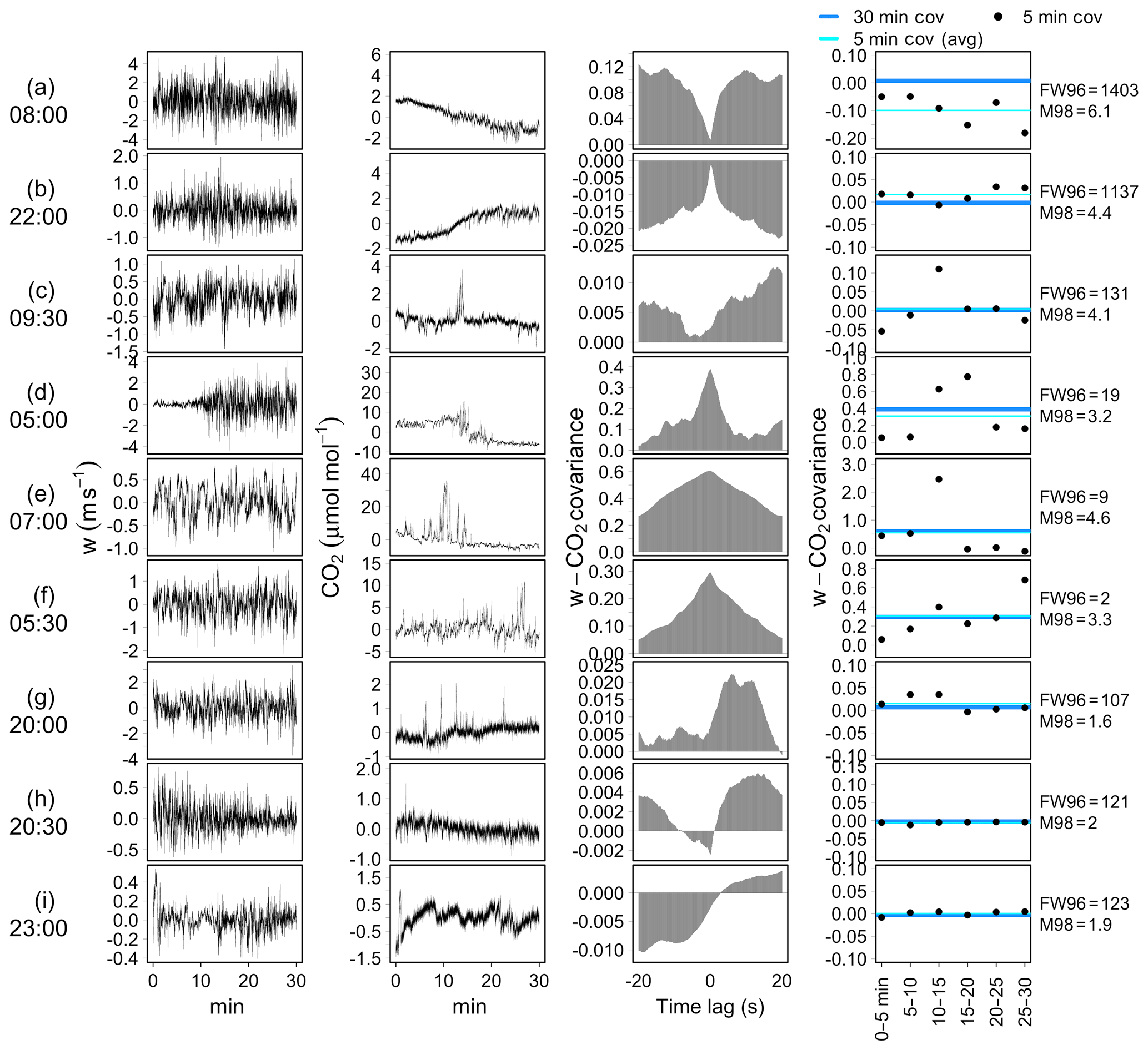
Figure 10Application of stationary tests to a selection of EC raw data collected at the FI-Hyy site. From left to right: vertical wind speed (w, m s−1); CO2 time series (µmol mol−1, after mean removal); cross-covariance function (CCF); comparison of 5 min covariances (black points), their average (cyan lines) and 30 min covariance (blue lines). FW96 and M98 test statistics are reported on the right-hand side.
3.2 Application of the data cleaning procedure
In this section we report the results of the data cleaning procedure based on the workflow depicted in Fig. 1 and including the application of QC tests described in Sect. 2. An illustrative example for NEE time series collected at the FI-Sii site during a period of 3 months is shown in Fig. 11 (for the other flux variables and for all the other sites, we refer the reader to the Sect. S4). The original time series had a rate of missing data of 12.3 %. The data cleaning procedure eliminated another 24.6 % of the data, for a total of 36.9 % resulting data gaps. In particular, 1.6 % of data were rejected after the removal of unreliable data caused by system malfunction and disturbances (Fig. 11b). A total of 3.6 % were removed due to low-signal-resolution problems (Fig. 11c). A total of 5.4 % were eliminated due to evidence of aberrant structural changes (Fig. 11d). The ITC test did not remove any data (Fig. 11e). An additional 10.6 % of data were removed because of non-stationary conditions (M98 test, Fig. 11f), and, finally, 1.6 % of fluxes were rejected because they were identified as both outlying and inheriting at least one ModEr (Fig. 11g).
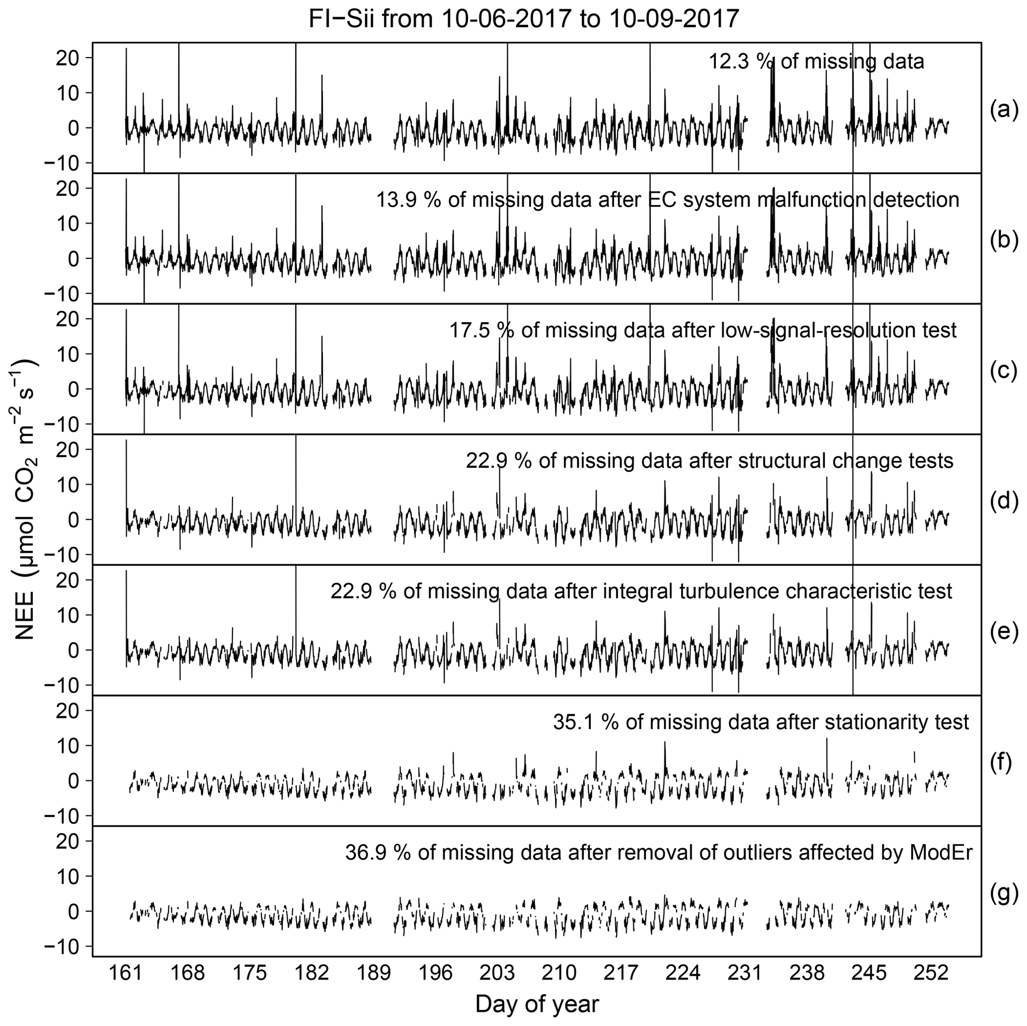
Figure 11Illustrative example of the sequential data cleaning procedure applied to NEE fluxes at the FI-Sii site.
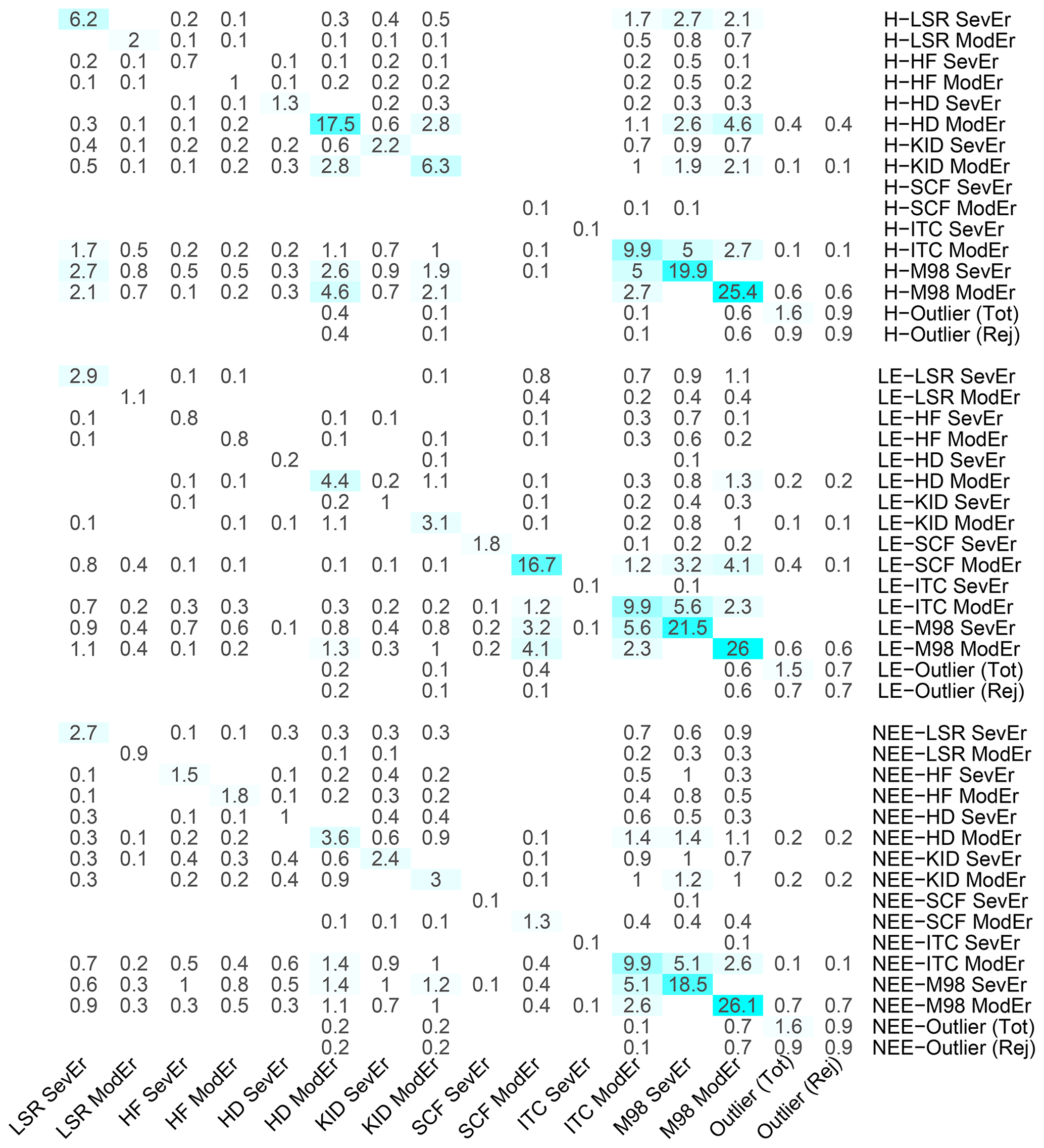
Figure 12Percentages of H, LE and NEE flux data affected by specific sources of systematic error according to several QC tests. Each cell of the matrix indicates the percentage of data receiving the status indicated in the ith row and the jth column; those on the diagonal refer to the percentage of data identified by each individual test. Empty cells indicate no data identified. Values are averaged across the 10 EC sites under investigation.
Figure 12 reports the percentages, averaged over the 10 sites under investigation, of H, LE and NEE flux data for which the QC tests returned ModEr and SevEr statements. The highest percentage of data inheriting a SevEr statement is caused by the lack of stationary conditions: irrespective of the flux variable, the percentage was around 20 %, with a maximum of 36.9 % for LE fluxes at the CH-Dav site and a minimum of 10.2 % for H fluxes at the SE-Htm site (see Sect. S4). With respect to the non-stationary test by M98, a further 25 % of fluxes inherited a ModEr statement. The percentage of data where the ITC test returned SevEr (ITC > 100 %) was only 0.1 %, while about 6 % received the status of ModEr.
Severe low-signal-resolution issues were identified only sporadically (in no more than 2.4 % of flux values), while a ModEr statement for the HDB test was inherited by 18 % of H values, due also to a moderate heteroscedasticity often observed in differenced sonic temperature time series. For all three flux variables, the percentage of outlying data was around 1.5 %. Approximately half of them received at least a ModEr statement from one of the QC tests and were therefore removed.
Figure 13 shows the STL decomposition of NEE time series at the FI-Sii site using the set of parameters described in Sect. 2.3.1. The ability of the modelling approach to separate the signal from the noise was assessed by evaluating the spectral characteristics of the irregular component by means of the Lomb–Scargle (LS) periodogram. In general, the periodogram did not show significant peaks, as exemplified for NEE in Fig. 13g and shown at length for all flux variables in Sect. S4. Despite the ability of the STL algorithm to reliably reproduce the complex correlation structure present in EC flux data, the irregular component was often heteroscedastic. This means that even if independent (since most of the serial correlation structure is removed), the irregular component is not identically distributed, i.e. its PDF changes over time. Such a property strongly limits the ability to use global threshold values above and below which data are identified as outliers.
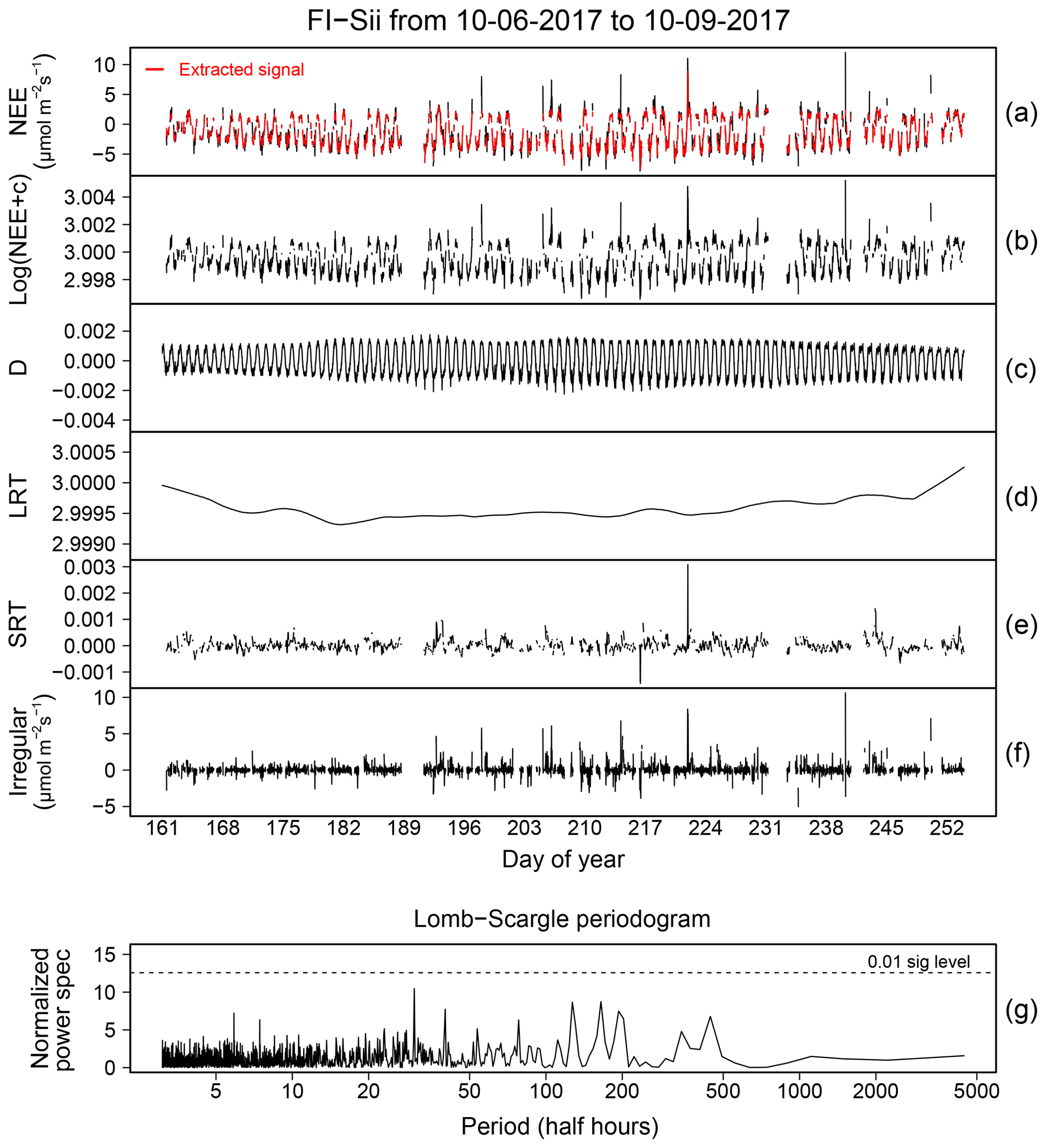
Figure 13Example of STL decomposition applied to NEE time series collected at the FI-Sii site. Panel (a) shows the original NEE flux data; (b) shows NEE after log10 transformation (c is a constant added to ensure the argument of log is positive); (c)–(f) show the diurnal cycle (D), the long-run trend (LRT), the short-run trend (SRT) and the irregular component of the STL algorithm (see Sect. 2.3.1 for more details). Notice that the irregular component is depicted after inverse log transformation. Panel (g) shows the Lomb–Scargle power spectral density estimate applied to the irregular component of STL decomposition. Dashed line indicates the 0.01 significance level.
Previous research (e.g. Richardson et al., 2012; Vitale et al., 2019a) has highlighted that the random error scales with the flux magnitude and that a Laplace distribution can better approximate the PDF of the random error. With this in mind, we grouped the values of the irregular component into 10 clusters of equal size, defined by percentiles of the signal estimated by the STL. This way, each cluster should contain values of the irregular component that are more likely to be identically distributed. Assuming a Laplace distribution and the (1−α) % confidence interval at the α=0.01 significance level, any values exceeding were detected as outliers (where σ was estimated using the Qn estimator of Rousseeuw and Croux, 1993). An illustrative example of this procedure is depicted in Fig. 14, where for simplicity the detail of only three clusters is reported.
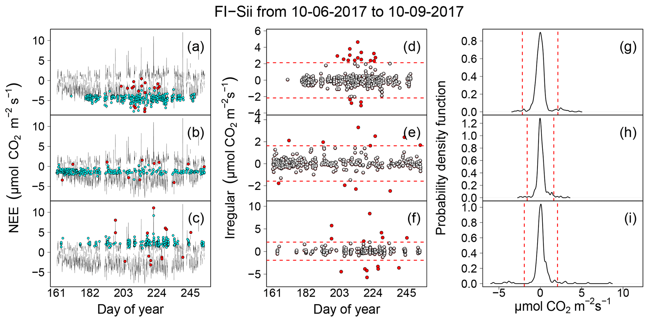
Figure 14Illustrative example of the outlier detection procedure applied to NEE fluxes at the FI-Sii site. NEE time series for the whole period (black lines) and selected flux values according to three deciles of the extracted signal (coloured points) are shown in (a)–(c). The corresponding values of the Irregular component are shown in (d)–(f), while their probability density functions are depicted in (g)–(i). Dashed red lines indicate the α-outlier regions (α=0.01) assuming a Laplace distribution. Red points indicate the detected outliers.
Quality control of eddy covariance flux datasets is challenging. The sources of systematic error responsible for introducing significant biases in the flux computation are manifold, and their correct identification is often made difficult by the masking effect induced by both the intrinsic stochastic properties (e.g. high degree of serial dependence, heteroscedasticity) and by the high level of noise characterizing raw data.
To take into account these features, new tests have been developed and included in a robust data cleaning procedure where the data rejection is articulated in two stages: the first stage involves the removal of any flux data for which at least one of the QC tests returned strong evidence of a specific source of systematic error (SevEr); the second stage consists of the removal of outlying fluxes, provided that at least one of the QC tests returned weak evidence of systematic error (ModEr) for the same flux value. Any flux data where all QC tests provided only negligible evidence of systematic error (NoEr) are never removed, even if they are later identified as outliers in the flux time series.
Although there is a strict relationship between the value of test statistics and the amount of bias affecting individual flux data, the interpretation of SevEr, ModEr and NoEr statements is performed in probabilistic terms, as the chances of a systematic error responsible for introducing bias in flux estimation. Consequently, the choice of threshold values used to assign the SevEr, ModEr and NoEr statements is to be interpreted as indicative of the margin of error associated with the result of a statistical test.
Compared to the existing classification schemes, the proposed approach does not aim at assigning a quality flag to flux data by combining the results of different QC tests. Rather, it aims at ensuring its scalability in order to facilitate the inclusion of new tests beyond those proposed in this paper. As for assigning a quality level to the retained data, we maintain that, given an unbiased flux estimate, a robust quantification of the random uncertainty would be the appropriate metric. Indeed, as a general principle, the larger the random uncertainty, the larger the amount of measurement error and, consequently, the lower the quality of the data. Assuming that flux data affected by systematic error have been avoided or removed via appropriate QA–QC procedures, the use of random uncertainty estimates as a quality indicator (1) would not constrain the QC test development, (2) would not preclude a classification of the data quality, if needed, and (3) would meet the requirements of advanced methods of analyses where interval estimates are more important than individual point estimates, such as in studies based on data assimilation techniques.
To this end, (global) uncertainty estimation procedures representative of the contribution of all possible sources of random error are required. They should include not only the contribution of random error caused by temporal and spatial sampling, but also those due to post-field data processing (e.g. the uncertainty related to the estimates of the spectral correction factors or those linked to the imputation model used to replace missing data). For such analyses, however, an essential prerequisite to achieve consistent results is the availability of unbiased, cleaned datasets. In this perspective, therefore, the data cleaning procedure proposed in this work constitutes an essential step in reducing the uncertainty of the results of subsequent analyses. Among these, also those aiming at providing a posteriori information about the presence of undetected/unknown sources of systematic error (e.g. those based on the evaluation of energy balance closure) can also benefit from less biased data.
In this study, the performance evaluation of each proposed test was carried out mainly by means of Monte Carlo simulations because they allow full control of (1) the time series dynamics (since the simulated autoregressive processes are stationary with a pre-fixed, reference correlation), (2) the presence of a specific source of systematic error and (3) the uncertainty due to the random error component. As a consequence, a proper evaluation of the bias effect caused by systematic errors and a more objective performance evaluation of the tests involved for their detection become feasible. Such evaluations are difficult to achieve with real, EC field data because the reference “true” value is unknown; therefore it is not possible to properly quantify the bias effect, and replicates are not available, making it difficult to evaluate the uncertainty associated with the estimates (either covariances and test statistics) due to the random error component. Developing a stochastic simulation model so complex as to include all the sources of error, both systematic and random, that are present in real-word EC time series data is a difficult task and is a target of ongoing work. Anyway, although the model generating the simulated data has a simple dynamic that can reproduce, at least in part, the behaviour of real EC data, if a QC test exhibits high false-positive and/or false-negative rates in such simple scenarios, it is most unlikely it will work properly with real data. In this case, the test would likely be methodologically robust but unusable in practice, affected by overinflated false-positive and false-negative errors.
Although there is still room for improvement, particularly in the development of more well-performing QC tests aiming at detecting violations of the main assumptions underlying the EC technique, we believe that the proposed data cleaning procedure can serve as a basis toward a unified QC strategy suitable for the centralized data processing pipelines, where the use of completely data-driven procedures that guarantee objectivity and reproducibility of the results constitutes an essential prerequisite.
RFlux software package (Vitale et al., 2019b) version 1.0.2 is available at https://github.com/icos-etc/RFlux (last access: 12 March 2020).
Access to benchmark data described in Sect. 2.5 is available from the Integrated Carbon Observation System (ICOS) Carbon Portal at https://data.icos-cp.eu/portal/ (ICOS RI, 2019).
The supplement related to this article is available online at: https://doi.org/10.5194/bg-17-1367-2020-supplement.
DV and DP conceived the study. DV organized the structure; selected, proposed and implemented the methodologies; and performed all the simulations, discussing the results with the coauthors. DV and GF wrote all the sections with the supervision of DP and with the contribution of all the coauthors. All authors reviewed the final manuscript, approved it and agreed on the submission.
The authors declare that they have no conflict of interest.
This research has been supported by the European Commission, H2020 Research Infrastructures (ENVRI PLUS (grant no. 654182), RINGO (grant no. 730944) and ENVRI-FAIR (grant no. 824068)).
This paper was edited by Martin De Kauwe and reviewed by Andrew Kowalski and one anonymous referee.
Aubinet, M., Chermanne, B., Vandenhaute, M., Longdoz, B., Yernaux, M., and Laitat, E.: Long term carbon dioxide exchange above a mixed forest in the Belgian Ardennes, Agr. Forest Meteorol., 108, 293–315, https://doi.org/10.1016/S0168-1923(01)00244-1, 2001. a
Aubinet, M., Vesala, T., and Papale, D. (Eds.): Eddy Covariance, Springer Netherlands, Dordrecht, https://doi.org/10.1007/978-94-007-2351-1, 2012. a
Box, G. E., Jenkins, G. M., Reinsel, G. C., and Ljung, G. M.: Time series analysis: forecasting and control, John Wiley & Sons, Hoboken, New Jersey, https://doi.org/10.2307/2284112, 2015. a
Cleveland, R. B., Cleveland, W. S., McRae, J. E., and Terpenning, I.: STL: A seasonal-trend decomposition, J. Off. Stat., 6, 3–73, 1990. a
Delpierre, N., Berveiller, D., Granda, E., and Dufrêne, E.: Wood phenology, not carbon input, controls the interannual variability of wood growth in a temperate oak forest, New Phytol., 210, 459–470, https://doi.org/10.1111/nph.13771, 2015. a
Donateo, A., Cava, D., and Contini, D.: A Case Study of the Performance of Different Detrending Methods in Turbulent-Flux Estimation, Bound.-Lay. Meteorol., 164, 19–37, https://doi.org/10.1007/s10546-017-0243-4, 2017. a
Finkelstein, P. L. and Sims, P. F.: Sampling error in eddy correlation flux measurements, J. Geophys. Res.-Atmos., 106, 3503–3509, https://doi.org/10.1029/2000JD900731, 2001. a
Foken, T. and Wichura, B.: Tools for quality assessment of surface-based flux measurements, Agr. Forest Meteorol., 78, 83–105, https://doi.org/10.1016/0168-1923(95)02248-1, 1996. a, b, c, d
Foken, T., Göockede, M., Mauder, M., Mahrt, L., Amiro, B., and Munger, W.: Post-Field Data Quality Control, in: Handbook of Micrometeorology, 181–208, Kluwer Academic Publishers, Dordrecht, https://doi.org/10.1007/1-4020-2265-4_9, 2004. a
Foken, T., Aubinet, M., and Leuning, R.: The Eddy Covariance Method, in: Eddy Covariance, 1–19, Springer Netherlands, Dordrecht, https://doi.org/10.1007/978-94-007-2351-1_1, 2012a. a
Foken, T., Leuning, R., Oncley, S. R., Mauder, M., and Aubinet, M.: Corrections and Data Quality Control, in: Eddy Covariance, 85–131, Springer Netherlands, Dordrecht, https://doi.org/10.1007/978-94-007-2351-1_4, 2012b. a, b, c
Foken, T., Babel, W., and Thomas, C.: Possible errors in flux measurements due to limited digitalization, Atmos. Meas. Tech., 12, 971–976, https://doi.org/10.5194/amt-12-971-2019, 2019. a
Franz, D., Acosta, M., Altimir, N., Arriga, N., Arrouays, D., Aubinet, M., Aurela, M., Ayres, E., López-Ballesteros, A., Barbaste, M., Berveiller, D., Biraud, S., Boukir, H., Brown, T., Brümmer, C., Buchmann, N., Burba, G., Carrara, A., Cescatti, A., Ceschia, E., Clement, R., Cremonese, E., Crill, P., Darenova, E., Dengel, S., D'Odorico, P., Gianluca, F., Fleck, S., Fratini, G., Fuß, R., Gielen, B., Gogo, S., Grace, J., Graf, A., Grelle, A., Gross, P., Grünwald, T., Haapanala, S., Hehn, M., Heinesch, B., Heiskanen, J., Herbst, M., Herschlein, C., Hörtnagl, L., Hufkens, K., Ibrom, A., Jolivet, C., Joly, L., Jones, M., Kiese, R., Klemedtsson, L., Kljun, N., Klumpp, K., Kolari, P., Kolle, O., Kowalski, A., Kutsch, W., Laurila, T., De Ligne, A., Linder, S., Lindroth, A., Lohila, A., Longdoz, B., Mammarella, I., Manise, T., Maranon-Jimenez, S., Matteucci, G., Mauder, M., Meier, P., Merbold, L., Mereu, S., Metzger, S., Migliavacca, M., Mölder, M., Montagnani, L., Moureaux, C., Nelson, D., Nemitz, E., Nicolini, G., Nilsson, M. B., Op de Beeck, M., Osborne, B., Ottosson Löfvenius, M., Pavelka, M., Peichl, M., Peltola, O., Pihlatie, M., Pitacco, A., Pokorny, R., Pumpanen, J., Ratié, C., Schrumpf, M., Sedlák, P., Serrano Ortiz, P., Siebicke, L., Šigut, L., Silvennoinen, H., Simioni, G., Skiba, U., Sonnentag, O., Soudani, K., Soulé, P., Steinbrecher, R., Tallec, T., Thimonier, A., Tuittila, E.-S., Tuovinen, J.-P., Vestin, P., Vincent, G., Vincke, C., Vitale, D., Waldner, P., Weslien, P., Wingate, L., Wohlfahrt, G., Zahniser, M., and Vesala, T.: Towards long-term standardised carbon and greenhouse gas observations for monitoring Europe's terrestrial ecosystems: a review, Int. Agrophys., 32, 439–455, https://doi.org/10.1515/intag-2017-0039, 2018. a
Fratini, G. and Mauder, M.: Towards a consistent eddy-covariance processing: an intercomparison of EddyPro and TK3, Atmos. Meas. Tech., 7, 2273–2281, https://doi.org/10.5194/amt-7-2273-2014, 2014. a
Fratini, G., Ibrom, A., Arriga, N., Burba, G., and Papale, D.: Relative humidity effects on water vapour fluxes measured with closed-path eddy-covariance systems with short sampling lines, Agr. Forest Meteorol., 165, 53–63, https://doi.org/10.1016/j.agrformet.2012.05.018, 2012. a
Fratini, G., Sabbatini, S., Ediger, K., Riensche, B., Burba, G., Nicolini, G., Vitale, D., and Papale, D.: Eddy covariance flux errors due to random and systematic timing errors during data acquisition, Biogeosciences, 15, 5473–5487, https://doi.org/10.5194/bg-15-5473-2018, 2018. a
Göckede, M., Foken, T., Aubinet, M., Aurela, M., Banza, J., Bernhofer, C., Bonnefond, J. M., Brunet, Y., Carrara, A., Clement, R., Dellwik, E., Elbers, J., Eugster, W., Fuhrer, J., Granier, A., Grünwald, T., Heinesch, B., Janssens, I. A., Knohl, A., Koeble, R., Laurila, T., Longdoz, B., Manca, G., Marek, M., Markkanen, T., Mateus, J., Matteucci, G., Mauder, M., Migliavacca, M., Minerbi, S., Moncrieff, J., Montagnani, L., Moors, E., Ourcival, J.-M., Papale, D., Pereira, J., Pilegaard, K., Pita, G., Rambal, S., Rebmann, C., Rodrigues, A., Rotenberg, E., Sanz, M. J., Sedlak, P., Seufert, G., Siebicke, L., Soussana, J. F., Valentini, R., Vesala, T., Verbeeck, H., and Yakir, D.: Quality control of CarboEurope flux data – Part 1: Coupling footprint analyses with flux data quality assessment to evaluate sites in forest ecosystems, Biogeosciences, 5, 433–450, https://doi.org/10.5194/bg-5-433-2008, 2008. a
Haapanala, S., Rinne, J., Pystynen, K.-H., Hellén, H., Hakola, H., and Riutta, T.: Measurements of hydrocarbon emissions from a boreal fen using the REA technique, Biogeosciences, 3, 103–112, https://doi.org/10.5194/bg-3-103-2006, 2006. a
Hafen, R.: Local regression models: advancements, applications, and new methods, PhD thesis, Purdue University, West Lafayette, 2010. a
Hafen, R.: stlplus: Enhanced Seasonal Decomposition of Time Series by
Loess, available at:
https://cran.r-project.org/web/packages/stlplus/index.html (last access: 12 March 2020),
R package version 0.5.1, 2019. a
Hyndman, R. J. and Athanasopoulos, G.: Forecasting: principles and practice, OTexts, Melbourne, Australia, available at: https://OTexts.com/fpp2 (last access: 12 March 2020), 2018. a
ICOS RI: Raw eddy covariance data from selected ICOS ecosystem stations, available at: https://www.icos-ri.eu, last access: 21 March 2019 (see code and data availability section for more info and data link). a, b
Kruijt, B., Elbers, J. A., von Randow, C., Araújo, A. C., Oliveira, P. J., Culf, A., Manzi, A. O., Nobre, A. D., Kabat, P., and Moors, E. J.: The robustness of eddy correlation fluxes for amazon rain forest conditions, Ecol. Appl., 14, 101–113, https://doi.org/10.1890/02-6004, 2004. a
Lagergren, F., Eklundh, L., Grelle, A., Lundblad, M., Molder, M., Harry, L., and Lindroth, A.: Net primary production and light use efficiency in a mixed coniferous forest in Sweden, Plant Cell Environ., 28, 412–423, https://doi.org/10.1111/j.1365-3040.2004.01280.x, 2005. a
Lasslop, G., Reichstein, M., Kattge, J., and Papale, D.: Influences of observation errors in eddy flux data on inverse model parameter estimation, Biogeosciences, 5, 1311–1324, https://doi.org/10.5194/bg-5-1311-2008, 2008. a
Lee, X., Massman, W., and Law, B. (Eds.): Handbook of Micrometeorology, Springer Netherlands, Dordrecht, https://doi.org/10.1007/1-4020-2265-4, 2005. a
LI-COR Biosciences: EddyPro 6.2.1: Help and User's Guide, LI-COR Biosciences, Lincoln, Nebraska USA, available at: https://www.licor.com/env/products/eddy_covariance/software.html (last access: 12 March 2020), 2019. a
Lomb, N. R.: Least-squares frequency analysis of unequally spaced data, Astrophys. Space Sci., 39, 447–462, https://doi.org/10.1007/bf00648343, 1976. a
Mahrt, L.: Flux sampling errors for aircraft and towers, J. Atmos. Ocean. Tech., 15, 416–429, https://doi.org/10.1175/1520-0426(1998)015<0416:fsefaa>2.0.co;2, 1998. a, b, c, d, e
Matteucci, M., Gruening, C., Ballarin, I. G., Seufert, G., and Cescatti, A.: Components, drivers and temporal dynamics of ecosystem respiration in a Mediterranean pine forest, Soil Biol. Biochem., 88, 224–235, https://doi.org/10.1016/j.soilbio.2015.05.017, 2015. a
Mauder, M. and Foken, T.: Documentation and instruction manual of the Eddy Covariance software package TK2, Univ Bayreuth, Abt Mikrometeorol, 26–42, available at: https://epub.uni-bayreuth.de/884/1/ARBERG026.pdf (last access: 12 March 2020), 2004. a, b
Mauder, M., Oncley, S. P., Vogt, R., Weidinger, T., Ribeiro, L., Bernhofer, C., Foken, T., Kohsiek, W., Bruin, H. A. R. D., and Liu, H.: The energy balance experiment EBEX-2000. Part II: Intercomparison of eddy-covariance sensors and post-field data processing methods, Bound.-Lay. Meteorol., 123, 29–54, https://doi.org/10.1007/s10546-006-9139-4, 2006. a
Mauder, M., Cuntz, M., Drüe, C., Graf, A., Rebmann, C., Schmid, H. P., Schmidt, M., and Steinbrecher, R.: A strategy for quality and uncertainty assessment of long-term eddy-covariance measurements, Agr. Forest Meteorol., 169, 122–135, https://doi.org/10.1016/j.agrformet.2012.09.006, 2013. a, b
Metzger, S., Durden, D., Sturtevant, C., Luo, H., Pingintha-Durden, N., Sachs, T., Serafimovich, A., Hartmann, J., Li, J., Xu, K., and Desai, A. R.: eddy4R 0.2.0: a DevOps model for community-extensible processing and analysis of eddy-covariance data based on R, Git, Docker, and HDF5, Geosci. Model Dev., 10, 3189–3206, https://doi.org/10.5194/gmd-10-3189-2017, 2017. a
Moncrieff, J., Malhi, Y., and Leuning, R.: The propagation of errors in long-term measurements of land-atmosphere fluxes of carbon and water, Glob. Change Biol., 2, 231–240, https://doi.org/10.1111/j.1365-2486.1996.tb00075.x, 1996. a
Moureaux, C., Debacq, A., Bodson, B., Heinesch, B., and Aubinet, M.: Annual net ecosystem carbon exchange by a sugar beet crop, Agr. Forest Meteorol., 139, 25–39, https://doi.org/10.1016/j.agrformet.2006.05.009, 2006. a
Nicolini, G., Aubinet, M., Feigenwinter, C., Heinesch, B., Lindroth, A., Mamadou, O., Moderow, U., Mölder, M., Montagnani, L., Rebmann, C., and Papale, D.: Impact of CO2 storage flux sampling uncertainty on net ecosystem exchange measured by eddy covariance, Agr. Forest Meteorol., 248, 228–239, https://doi.org/10.1016/j.agrformet.2017.09.025, 2018. a, b
Pilegaard, K., Ibrom, A., Courtney, M. S., Hummelshøj, P., and Jensen, N. O.: Increasing net CO2 uptake by a Danish beech forest during the period from 1996 to 2009, Agr. Forest Meteorol., 151, 934–946, https://doi.org/10.1016/j.agrformet.2011.02.013, 2011. a
Rannik, Ü. and Vesala, T.: Autoregressive filtering versus linear detrending in estimation of fluxes by the eddy covariance method, Bound.-Lay. Meteorol., 91, 259–280, https://doi.org/10.1023/A:1001840416858, 1999. a
R Development Core Team: R: A Language and Environment for Statistical Computing, R Foundation for Statistical Computing, Vienna, Austria, ISBN 3-900051-07-0, http://www.R-project.org (last access: 12 March 2020), 2019. a
Rebmann, C., Aubinet, M., Schmid, H., Arriga, N., Aurela, M., Burba, G., Clement, R., Ligne, A. D., Fratini, G., Gielen, B., Grace, J., Graf, A., Gross, P., Haapanala, S., Herbst, M., Hörtnagl, L., Ibrom, A., Joly, L., Kljun, N., Kolle, O., Kowalski, A., Lindroth, A., Loustau, D., Mammarella, I., Mauder, M., Merbold, L., Metzger, S., Mölder, M., Montagnani, L., Papale, D., Pavelka, M., Peichl, M., Roland, M., Serrano-Ortiz, P., Siebicke, L., Steinbrecher, R., Tuovinen, J.-P., Vesala, T., Wohlfahrt, G., and Franz, D.: ICOS eddy covariance flux-station site setup: a review, Int. Agrophys., 32, 471–494, https://doi.org/10.1515/intag-2017-0044, 2018. a
Richardson, A. D., Mahecha, M. D., Falge, E., Kattge, J., Moffat, A. M., Papale, D., Reichstein, M., Stauch, V. J., Braswell, B. H., Churkina, G., Kruijt, B., and Hollinger, D. Y.: Statistical properties of random CO2 flux measurement uncertainty inferred from model residuals, Agr. Forest Meteorol., 148, 38–50, https://doi.org/10.1016/j.agrformet.2007.09.001, 2008. a
Richardson, A. D., Aubinet, M., Barr, A. G., Hollinger, D. Y., Ibrom, A., Lasslop, G., and Reichstein, M.: Uncertainty Quantification, in: Eddy Covariance, edited by: Aubinet, M., Vesala, T., and Papale, D., 173–209, Springer Netherlands, Dordrecht, https://doi.org/10.1007/978-94-007-2351-1_7, 2012. a, b, c, d, e, f
Rousseeuw, P. J. and Croux, C.: Alternatives to the Median Absolute Deviation, J. Am. Stat. Assoc., 88, 1273–1283, https://doi.org/10.1080/01621459.1993.10476408, 1993. a, b, c
Sabbatini, S. and Papale, D.: ICOS Ecosystem Instructions for Turbulent Flux Measurements of CO2, Energy and Momentum (Version 20180110), ICOS Ecosystem Thematic Centre, https://doi.org/10.18160/qwv4-639g, 2017. a
Sabbatini, S., Mammarella, I., Arriga, N., Fratini, G., Graf, A., Hörtnagl, L., Ibrom, A., Longdoz, B., Mauder, M., Merbold, L., Metzger, S., Montagnani, L., Pitacco, A., Rebmann, C., Sedlák, P., Šigut, L., Vitale, D., and Papale, D.: Eddy covariance raw data processing for CO2 and energy fluxes calculation at ICOS ecosystem stations, Int. Agrophys., 32, 495–515, https://doi.org/10.1515/intag-2017-0043, 2018. a, b
Sandborn, V. A.: Measurements of intermittency of turbulent motion in a boundary layer, J. Fluid Mech., 6, 221, https://doi.org/10.1017/s0022112059000581, 1959. a
Scargle, J. D.: Studies in astronomical time series analysis. II – Statistical aspects of spectral analysis of unevenly spaced data, Astrophys. J., 263, 835, https://doi.org/10.1086/160554, 1982. a
Schmidt, M., Reichenau, T. G., Fiener, P., and Schneider, K.: The carbon budget of a winter wheat field: An eddy covariance analysis of seasonal and inter-annual variability, Agr. Forest Meteorol., 165, 114–126, https://doi.org/10.1016/j.agrformet.2012.05.012, 2012. a
Suni, T., Rinne, J., Reissell, A., Altimir, N., Keronen, P., Rannik, U., Maso, M., Kulmala, M., and Vesala, T.: Long-term measurements of surface fluxes above a Scots pine forest in Hyytiälä, southern Finland, 1996–2001, Boreal Environ. Res., 8, 287–302, 2003. a
Thomas, C. K., Law, B. E., Irvine, J., Martin, J. G., Pettijohn, J. C., and Davis, K. J.: Seasonal hydrology explains interannual and seasonal variation in carbon and water exchange in a semiarid mature ponderosa pine forest in central Oregon, J. Geophys. Res., 114, G04006, https://doi.org/10.1029/2009jg001010, 2009. a
van Meeningen, Y., Wang, M., Karlsson, T., Seifert, A., Schurgers, G., Rinnan, R., and Holst, T.: Isoprenoid emission variation of Norway spruce across a European latitudinal transect, Atmos. Environ., 170, 45–57, https://doi.org/10.1016/j.atmosenv.2017.09.045, 2017. a
Vickers, D. and Mahrt, L.: Quality Control and Flux Sampling Problems for Tower and Aircraft Data, J. Atmos. Ocean. Tech., 14, 512–526, https://doi.org/10.1175/1520-0426(1997)014<0512:QCAFSP>2.0.CO;2, 1997. a, b
Vitale, D., Bilancia, M., and Papale, D.: Modelling random uncertainty of eddy covariance flux measurements, Stoch. Env. Res. Risk A., 33, 725–746, https://doi.org/10.1007/s00477-019-01664-4, 2019a. a, b, c
Vitale, D., Papale, D., and ICOS-ETC Team: RFlux: An R Package for Processing and Cleaning Eddy Covariance Flux Measurements, ICOS-ETC, Viterbo, Italy, available at: https://github.com/icos-etc/RFlux (last access: 12 March 2020), R package version 1.0.2, 2019b. a, b
Westfall, P. H.: Kurtosis as Peakedness, 1905–2014. R.I.P., Am. Stat., 68, 191–195, https://doi.org/10.1080/00031305.2014.917055, 2014. a
Wollschläger, U., Attinger, S., Borchardt, D., Brauns, M., Cuntz, M., Dietrich, P., Fleckenstein, J. H., Friese, K., Friesen, J., Harpke, A., Hildebrandt, A., Jäckel, G., Kamjunke, N., Knöller, K., Kögler, S., Kolditz, O., Krieg, R., Kumar, R., Lausch, A., Liess, M., Marx, A., Merz, R., Mueller, C., Musolff, A., Norf, H., Oswald, S. E., Rebmann, C., Reinstorf, F., Rode, M., Rink, K., Rinke, K., Samaniego, L., Vieweg, M., Vogel, H.-J., Weitere, M., Werban, U., Zink, M., and Zacharias, S.: The Bode hydrological observatory: a platform for integrated, interdisciplinary hydro-ecological research within the TERENO Harz/Central German Lowland Observatory, Environ. Earth Sci., 76, 29, https://doi.org/10.1007/s12665-016-6327-5, 2017. a
Zielis, S., Etzold, S., Zweifel, R., Eugster, W., Haeni, M., and Buchmann, N.: NEP of a Swiss subalpine forest is significantly driven not only by current but also by previous year's weather, Biogeosciences, 11, 1627–1635, https://doi.org/10.5194/bg-11-1627-2014, 2014. a