the Creative Commons Attribution 4.0 License.
the Creative Commons Attribution 4.0 License.
 | 11 Jul 2019
What drives the latitudinal gradient in open-ocean surface dissolved inorganic carbon concentration?
Mathis P. Hain
Matthew P. Humphreys
Sue Hartman
Toby Tyrrell
Previous work has not led to a clear understanding of the causes of spatial pattern in global surface ocean dissolved inorganic carbon (DIC), which generally increases polewards. Here, we revisit this question by investigating the drivers of observed latitudinal gradients in surface salinity-normalized DIC (nDIC) using the Global Ocean Data Analysis Project version 2 (GLODAPv2) database. We used the database to test three different hypotheses for the driver producing the observed increase in surface nDIC from low to high latitudes. These are (1) sea surface temperature, through its effect on the CO2 system equilibrium constants, (2) salinity-related total alkalinity (TA), and (3) high-latitude upwelling of DIC- and TA-rich deep waters. We find that temperature and upwelling are the two major drivers. TA effects generally oppose the observed gradient, except where higher values are introduced in upwelled waters. Temperature-driven effects explain the majority of the surface nDIC latitudinal gradient (182 of the 223 µmol kg−1 increase from the tropics to the high-latitude Southern Ocean). Upwelling, which has not previously been considered as a major driver, additionally drives a substantial latitudinal gradient. Its immediate impact, prior to any induced air–sea CO2 exchange, is to raise Southern Ocean nDIC by 220 µmol kg−1 above the average low-latitude value. However, this immediate effect is transitory. The long-term impact of upwelling (brought about by increasing TA), which would persist even if gas exchange were to return the surface ocean to the same CO2 as without upwelling, is to increase nDIC by 74 µmol kg−1 above the low-latitude average.


The ocean absorbs about one-quarter of the anthropogenic CO2 emitted every year (Le Quéré et al., 2018). It is the largest non-geological carbon reservoir (∼38 000 Gt C; Falkowski et al., 2000), containing 50 times as much carbon as the pre-industrial atmosphere, and thereby modulates the Earth's climate system. Approximately 97 % of the carbon in the ocean is in the form of dissolved inorganic carbon (DIC), which is the total concentration of aqueous CO2 and bicarbonate and carbonate ions:
where [] refers to the sum of aqueous CO2 and undissociated carbonic acid (H2CO3), with the latter being negligible (Zeebe and Wolf-Gladrow, 2001).
Understanding what controls the distribution of oceanic DIC is essential for quantifying anthropogenic CO2 invasion (e.g., Gruber, 1998; Humphreys et al., 2016; Lee et al., 2003; Sabine et al., 1999, 2002; Vázquez-Rodríguez et al., 2009) and consequent ocean acidification (e.g., Doney et al., 2009; Orr et al., 2005). As most marine organisms live in the sunlit surface ocean, where CO2 exchange with the atmosphere happens, the controls on surface ocean DIC in particular merit investigation.
Many previous studies focused on the vertical, rather than latitudinal, distribution of DIC. They investigated the contributions of the different “carbon pumps” – solubility pump, soft tissue pump, and carbonate pump (Cameron et al., 2005; Gruber and Sarmiento, 2002; Toggweiler et al., 2003a, b) – to the pattern of DIC with depth. The solubility pump is based on the assumption that, at high latitudes where deep waters form, DIC is high because the low water temperature increases CO2 solubility. Lee et al. (2000) used this principle to predict salinity-normalized DIC (nDIC) from empirical functions of sea surface temperature and nitrate that varied seasonally and geographically.
Key et al. (2004) depicted the global distribution of surface DIC using an earlier version (GLODAPv1) of the dataset than we used in this study, noting that the surface DIC pattern is more similar to nutrients (including in the Southern Ocean, where both DIC and nutrients are enriched) than to salinity – unlike total alkalinity (TA), whose pattern more closely resembles that of salinity (Fry et al., 2015). Using the data from the new GLODAPv2 database (Key et al., 2015; Olsen et al., 2016), surface DIC is confirmed here to have its highest values at high latitudes, like nutrients, and to reach its lowest values at low latitudes in each basin (Fig. 1a; more details in Sect. 3.1). Earlier studies (Lee et al., 2000; Toggweiler et al., 2003a; Williams and Follows, 2011, Sect. 6.3 “What controls DIC in the surface ocean?”) suggested that temperature is of primary importance in regulating surface DIC (e.g., Lee et al., 2000; Toggweiler et al., 2003a; Williams and Follows, 2011; Humphreys, 2017). Under this assumption, surface waters in cool regions at high latitudes should hold more DIC than surface waters in the warm regions at low latitudes.
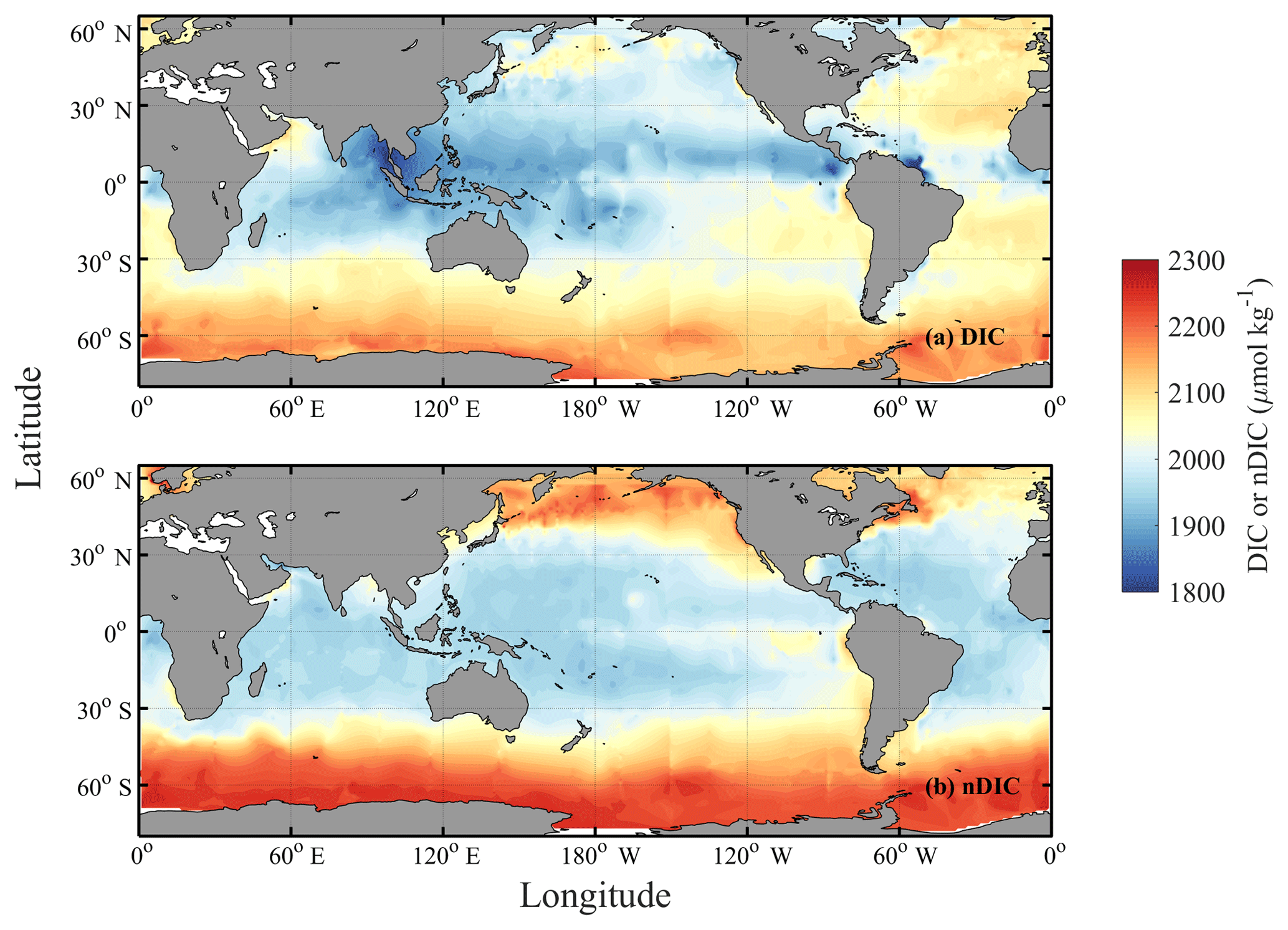
Figure 1Spatial distributions of DIC and nDIC. (a) DIC (normalized to year 2005); (b) salinity-normalized DIC (nDIC, DIC normalized to reference year of 2005 and salinity of 35) in the surface global ocean. The latitudinal trends are clear, particularly for nDIC.
Williams and Follows (2011) argued that another variable also exerts control on the surface DIC distribution: TA sets the equilibrium capacity for seawater to hold DIC in solution (Omta et al., 2011; Humphreys et al., 2018), so higher surface TA values may lead to higher DIC. Takahashi et al. (2014) explored the seasonal distribution of climatological surface DIC using seawater pCO2 from the Lamont Doherty Earth Observatory (LDEO) database and TA estimated from salinity, qualitatively attributing seasonal differences (on a regional scale) to the greater upward mixing of high-CO2 deep waters in winter and summer biological carbon drawdown. They noted the potential for upwelling to alter surface DIC, but focused on DIC seasonality rather than its spatial variability. In recent years, the global surface DIC database has greatly expanded (e.g., Bates et al., 2006; Sasse et al., 2013), culminating in GLODAPv2 (Key et al., 2015; Olsen et al., 2016; Lauvset et al., 2016), but the drivers of the global surface DIC distribution have not yet been reassessed.
The processes that influence the distribution of surface DIC at the local scale can be divided into those which change DIC by direct addition or removal, and those which affect DIC indirectly. The direct processes include (1) biological carbon assimilation during primary production and release during remineralization (Bozec et al., 2006; Clargo et al., 2015; Toggweiler et al., 2003b; Yasunaka et al., 2013); (2) transport of DIC-rich deep waters into the surface layer (Jiang et al., 2013; Lee et al., 2000); and (3) production and export of CaCO3. Indirect processes include (4) seawater dilution or concentration due to precipitation or evaporation (Friis et al., 2003); (5) warming and cooling, which alter CO2 solubility and induce air–sea gas exchange that acts to reduce air–sea CO2 disequilibrium (Bozec et al., 2006; Toggweiler et al., 2003a; Williams and Follows, 2011); and (6) the above processes (1–4) through their impact on TA – if high/low TA values are not matched by high/low DIC values then the resulting low/high seawater pCO2 stimulates CO2 ingassing/outgassing until DIC matches TA (Humphreys et al., 2018). The effects of equilibrium processes (the effects through temperature and upwelled TA) change the surface ocean DIC at which air–sea CO2 equilibrium occurs, so these effects can persist beyond the air–sea CO2 equilibrium timescale (months to a year; Jones et al., 2014). The effects of disequilibrium processes, such as direct DIC supply from upwelling, and biological uptake of DIC in response to upwelled nutrients (principally iron; Moore et al., 2016) can persist no longer than the CO2 equilibrium timescale.
Our study builds on previous work in several ways. First, whereas many previous studies looked to understand the vertical DIC distribution, our target is to understand the latitudinal surface DIC distribution. Second, we identify the most important processes, not just the variables, driving the surface DIC distribution (Fig. 2). Third, we use a much larger observational global dataset – GLODAPv2.

Figure 2Major controls on surface DIC. Schematic showing the main processes exerting an influence over the concentration of DIC in the global surface ocean (producing variation with latitude). Blue shapes are processes and orange shapes are variables. Straight solid arrows represent equilibrium processes regulating DIC in the long term and wavy solid arrows represent disequilibrium processes regulating DIC in the short term. In the paper, we evaluate the upwelling effect on surface DIC in the Southern Ocean. Dashed arrows with text denote the three different ways that upwelling affects DIC: the direct effect through upwelled DIC, the indirect effect through upwelled nutrients which stimulate biological removal of DIC, and the indirect effect through upwelled TA changing the equilibrium DIC with the atmosphere.
We evaluate three main hypotheses as to which processes cause the increase in surface DIC and nDIC from low to high latitude (Fig. 1):
-
latitudinal variation in solar heating via its effect on sea surface temperature, and hence CO2 solubility;
-
evaporation and precipitation, through their effects on TA; and
-
upwelling and winter entrainment through the introduction of DIC- and TA-rich deep waters to the (sub)polar surface oceans, when coupled with iron limitation of biological uptake of DIC.
It is easier to constrain the dynamics of upwelling and quantify their impact on surface DIC in the Southern Ocean (where upwelling has been more comprehensively studied; e.g., Marshall and Speer, 2012; Morrison et al., 2015) than in the subarctic North Atlantic and North Pacific oceans (where upward transport occurs via deep mixing in the winter, combined with upwelling in the North Pacific). The Southern Ocean also plays a crucial role in the global overturning circulation (e.g., Marshall and Speer, 2012), and the global carbon cycle (Landschützer et al., 2015; Mikaloff-Fletcher, 2015). Therefore, we focused on the Southern Ocean for the evaluation of the third hypothesis. A novel conclusion of this study is that upwelling, whose global significance has previously been overlooked, is very important in shaping the spatial distribution of surface ocean DIC, in part because upwelling of TA changes equilibrium DIC.
We used data from GLODAPv2 (Key et al., 2015; Olsen et al., 2016). This compilation contains data from over 700 cruises conducted from 1972 to 2013, with about a third collected since 2003. The data have undergone secondary quality control and have been adjusted for consistency (Key et al., 2015; Lauvset and Tanhua, 2015; Olsen et al., 2016).
2.1 Data processing
We define the “surface” ocean as the uppermost 30 m at latitudes greater than 30∘, and shallower than 20 m at latitudes less than 30∘ (following e.g., Fry et al., 2015; Lee et al., 2006). Only open-ocean data (water depth > 200 m) were included in this study (Fig. 3).

Figure 3Spatial and temporal distribution of GLODAPv2 sampling stations (with Arctic and Mediterranean Sea data removed).
We excluded regions perturbed by river inputs in order to remove confounding factors affecting the latitudinal distributions of DIC and nDIC on smaller length scales than investigated here. We excluded the Arctic Ocean (> 65∘ N) (Fig. 3) because it is heavily influenced by river inputs (Fry et al., 2015; Jiang et al., 2014), all data from the Mediterranean Sea and the Red Sea because of their very high salinity (Jiang et al., 2014), and some data (those where S is less than 34) from other ocean areas: the Amazon River plume in the North Atlantic (5–10∘ N, > 45∘ W), the Ganges–Brahmaputra plume in the Bay of Bengal (> 5∘ N, 80–94∘ E) (both Fry et al., 2015) and the western North Atlantic margins (Cai et al., 2010). We also excluded low-latitude ocean areas affected by upwelling (i.e., the eastern equatorial Pacific and northern Californian upwelling regions).
Because atmospheric CO2 increased during the period when the GLODAPv2 data were collected (1972–2013), DIC has also increased in surface waters (Bates et al., 2014). To prevent temporal DIC trends from generating artificial spatial variability, we normalized surface DIC to a reference year of 2005, by assuming that surface seawater pCO2 tracks atmospheric pCO2 (Feely, 2008; see also CO2 time series in the North Pacific at https://pmel.noaa.gov/co2/file/CO2+time+series, last access: 30 January 2019). We first calculated the change in atmospheric mole fraction of CO2 (xCO2,air) from the reference year 2005:
where the superscript “t” and “2005” refer to year, and the globally averaged atmospheric xCO2 data can be found at https://www.esrl.noaa.gov/gmd/ccgg/trends/, last access: 30 January 2019 (neither spatial nor seasonal variability in atmospheric CO2 is taken into account; the associated error in surface DIC is less than 2 µmol kg−1).
Then we converted ΔxCO2,air into ΔpCO2,air (Takahashi et al., 2009) just above the sea surface, using calculated humidity data. It is then assumed that ΔpCO2,sw, representing the change in sea surface pCO2 relative to the year 2005, is equal to ΔpCO2,air.
Therefore the sea surface pCO2 normalized to year 2005 was calculated as
where was calculated from in situ DIC, TA, temperature, and salinity using CO2SYS v1.1 (van Heuven et al., 2011; dissociation constants used are described in Sect. 2.3).
Since the anthropogenic CO2 perturbation does not change TA, DIC normalized to the year 2005 was calculated with inputs of in situ TA and using CO2 SYS (van Heuven et al., 2011):
The concentration of DIC hereinafter refers to DIC normalized to the year 2005.
2.2 Salinity normalization
Salinity normalization was used to correct for the influence of precipitation and evaporation in the open ocean (Postma, 1964). Data were normalized to a reference salinity of 35 using a standard procedure:
where nX refers to the normalized variable, Xobs is the observed value of the variable, and Sobs is the observed salinity.
We acknowledge that this approach (Eq. 5) can create artificial variance in DIC distribution (Friis et al., 2003) because it ignores the influences of riverine input and upwelling from below the thermocline. We avoided the riverine problem by excluding affected regions (Sect. 2.1). We found that correcting for the “non-zero intercept” of DIC–salinity plots (Friis et al., 2003) in different ocean basins has negligible influence on salinity normalization of DIC, accounting for at most 7 µmol kg−1 change in DIC; upwelling from below the thermocline also has negligible influence, accounting for at most 4 µmol kg−1 change in DIC. These changes are small compared to the DIC latitudinal gradient of about 200 µmol kg−1 that we investigate here.
2.3 Carbonate chemistry
Carbonate system variables were calculated from DIC and TA using version 1.1 of CO2SYS for MATLAB (van Heuven et al., 2011). The dissociation constants for carbonic acid and bisulfate were taken from Lueker et al. (2000) and Dickson (1990), respectively, and the total borate–salinity relationship was taken from Lee et al. (2010).
2.4 Calculation of DIC and nDIC latitudinal gradients
The magnitude of the latitudinal gradient depends on the time of year because it is calculated from DIC values that are higher in winter at high altitudes. The seasonal amplitude of surface nDIC varies over the global open ocean. It is generally small at low latitudes: ∼20 µmol kg−1 in the subtropical Pacific Ocean (Keeling et al., 2004) and ∼40 µmol kg−1 in the subtropical Atlantic Ocean (Bates et al., 1996). It is much larger at some (but not all) high-latitude locations: ∼113 µmol kg−1 in the northwestern Pacific Ocean (Kawakami et al., 2007) and ∼60 µmol kg−1 in the subarctic northeast Pacific Ocean (Wong et al., 2002), but only ∼25 µmol kg−1 at the KERFIX site in the Southern Ocean (Louanchi et al., 1999). Because most ship-collected data (as contained in GLODAPv2) are collected in spring or summer months, the latitudinal gradients averaged across the whole year will be larger in some locations than presented here, and the magnitudes of the latitudinal gradients presented here should be considered lower estimates. For instance, the observed nDIC difference (ΔnDIC) between the North Pacific (40–60∘ N) and low latitudes (30∘ S–30∘ N) is 171 µmol kg−1 when calculated from summer data only and 224 µmol kg−1 when calculated from winter data only. For the Southern Ocean, ΔnDIC is 214 µmol kg−1 in summer and 240 µmol kg−1 in winter. This sensitivity to time of year should be noted but is not considered further here because it is relatively small compared to the overall magnitude of ΔnDIC.
2.5 Calculations of the effects of various processes on DIC
The second hypothesis (evaporation and precipitation through their effects on TA) was evaluated by salinity normalization (Eq. 5). The methods for calculating the impacts of the other two processes on the surface DIC concentration are now explained. The effect of upwelling is evaluated in the Southern Ocean, from both short- and long-term perspectives. In addition, we also quantify the effect of iron limitation, which would potentially affect the observed (n)DIC distribution.
2.5.1 SST-driven effect
The temperature effect on the carbonate system has two aspects. First, when water temperature increases, the equilibria between carbonate species (Eq. 6) shift towards increasing the aqueous CO2 and carbonate ion concentrations (Dickson and Millero, 1987):
Second, CO2 solubility is lower at higher temperatures and vice versa (Weiss, 1974). Neither effect alters DIC directly, but both change the seawater pCO2. A larger proportion of DIC exists as aqueous CO2 at higher temperatures and the ratio of pCO2 to [CO2] also increases as solubility decreases (Eq. 7, Henry's law):
where KH is the Henry's constant (solubility) for CO2.
Both effects tend to increase sea surface pCO2 as seawater warms, potentially increasing the net sea-to-air CO2 flux; the induced outgassing of CO2 reduces sea surface pCO2 and DIC as it shifts the system towards CO2 equilibrium. Therefore, for an open-ocean system in contact with the atmosphere, sea surface temperature (SST) can control the DIC distribution, and this can by itself produce DIC latitudinal variations.
To examine the magnitude of the expected temperature-induced DIC changes, we chose the low-latitude area as the reference, then removed the latitudinal SST variation and recalculated the open-ocean surface DIC everywhere for a constant SST of 27 ∘C (the mean sea surface temperature in the subtropics from 30∘ S to 30∘ N). We first calculated the in situ pCO2 from observed SST, SSS (sea surface salinity), TA, and DIC using CO2SYS. The calculated pCO2 from TA and DIC has been found to agree well with the measured pCO2 by Takahashi et al. (2014) (root-mean-square deviation of ±6.8 µatm). We then altered the sea surface temperature from its in situ value to 27 ∘C, which would change the solubility of CO2 and induce air–sea CO2 gas exchange. Then air–sea CO2 gas exchange (which does not change TA) was assumed to proceed until pCO2 was back to the same level as before resetting the temperature. Next, we used CO2SYS to calculate DICSST=27 (Table 1) based on an input temperature of 27 ∘C, observed salinity and TA, and the in situ pCO2 calculated as above. DICSST=27 thus represents temperature-normalized DIC, and should exhibit the same spatial variability as DIC except that the temperature-induced component of the variability has been removed. Finally, the difference between observed DIC and DICSST=27 gives the DIC variation attributed to temperature variation (see Table 1 for definitions of each term):
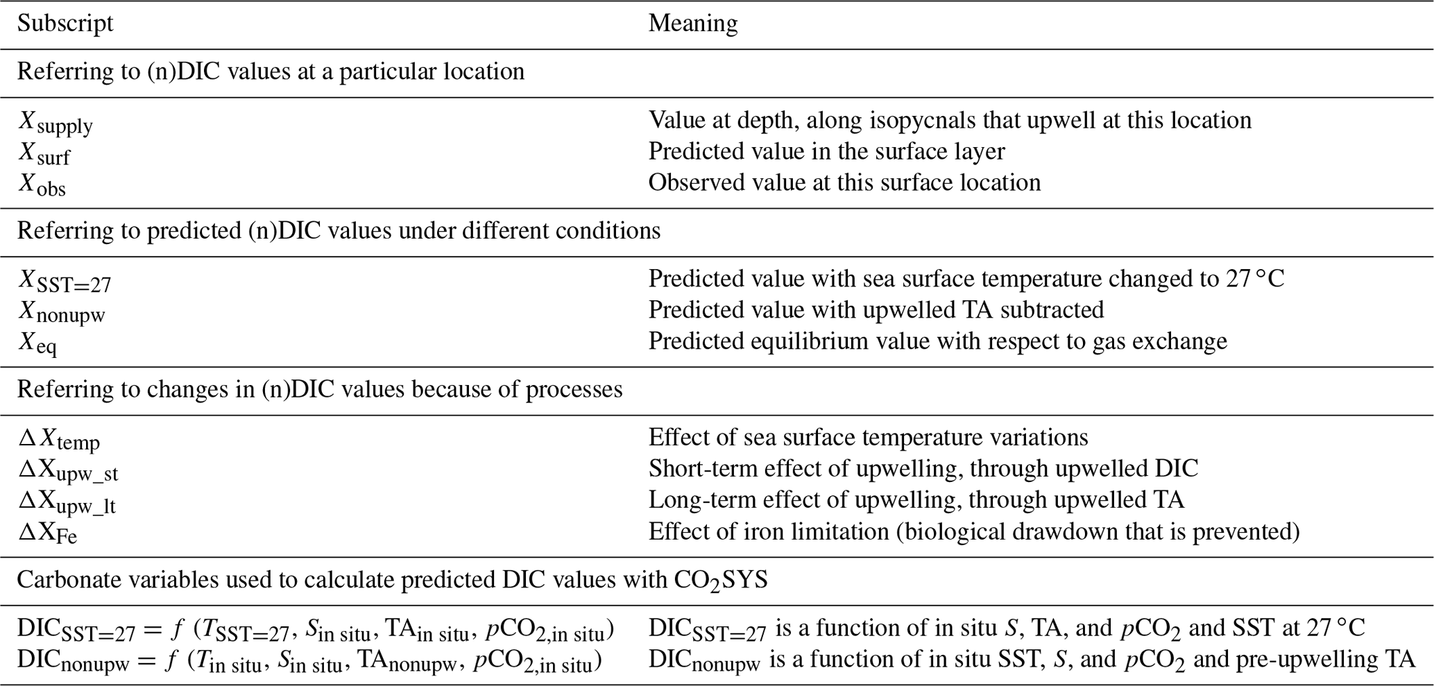
Table 1Definitions of subscripts and main terms used in the text. X represents any variable involved in the calculations. The program CO2SYS was used to calculate values under different conditions.
The same procedure was followed for calculating ΔnDICtemp:
2.5.2 Upwelled DIC-driven effect (short-term effect of upwelling)
Upwelling of DIC-rich subsurface waters can increase the surface DIC. The largest upwelling flux anywhere in the world takes place in the Southern Ocean (Talley, 2013). Subsurface waters in the Southern Ocean upwell along the neutral density isopycnals of 27.6, 27.9, and 27.9 kg m−3 in the southern Atlantic, Indian, and Pacific oceans, respectively (Ferrari et al., 2014; Lumpkin and Speer, 2007; Marshall and Speer, 2012; Talley, 2013).
Upwelling occurs within the Antarctic Circumpolar Current (ACC) where the wind stress is greatest (Morrison et al., 2015). As the upwelled water subsequently advects away, the effects of upwelling on DIC are transported to nearby locations. Therefore, instead of a direct supply from deep to surface locations such as L3 (Fig. 4), DIC is brought to the subsurface primarily along isopycnals (shown in Fig. 4 as the black curve to L1), finally reaching the surface at L2. Then, the upwelled waters with enriched DIC, TA, and nutrients feed both branches of the Southern Ocean overturning circulation. One branch is transported northwards via Ekman transport from L2 to L3, as shown by the black arrow towards the Equator, and the other is recycled to form Antarctic Bottom Water (AABW) (Talley, 2013). The effect of upwelling on sea surface temperature is negligible and not considered here because both deep water and high-latitude surface waters have similarly low temperatures.
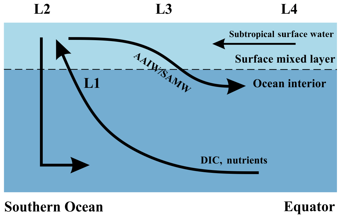
Figure 4A schematic illustrating locations of interest and assumed major flow paths in the Southern Ocean. Black arrows represent the flow directions of water masses. The lower curved arrow denotes upwelling of deep water along isopycnal surfaces, and the upper curved arrow denotes subduction to form Subantarctic Mode Water (SAMW) and Antarctic Intermediate Water (AAIW). L1: upwelling water below the mixed layer, prior to any influence of surface processes; L2: sea surface within the core of the Southern Ocean upwelling south of 50∘ S (Morrison et al., 2015); L3: sea surface from 30 to 50∘ S; L4: sea surface north of 30∘ S, which experiences no direct effects from upwelling in the Southern Ocean.
We first consider the increase in DIC induced by the upwelling of deep water with high DIC concentrations. While some of the initial increase is usually removed shortly afterwards by biological export fueled by the nutrients brought up at the same time, excess DIC remains if the subsequent biological removal of DIC does not match the initial increase. Phosphorus has the simplest nutrient behavior in the ocean with only one significant source to the ocean as a whole (river input) and one major sink (organic matter burial) (Ruttenberg, 2003; Tyrrell, 1999). In this study, the salinity-normalized phosphate (nPhos) concentration was used as a proxy for calculating how much salinity-normalized DIC (nDIC) was upwelled along with it and not yet removed again by biological uptake of phosphate and DIC. We used salinity-normalized concentrations to correct for the influence of precipitation (rainfall) that dilutes DIC and phosphate concentrations in proportion to the effects on salinity (Eq. 5). In this calculation, it was assumed that the only external source of phosphate to surface waters is from upwelling and the only subsequent loss is through export of organic matter, leading to the equation:
where the subscript “supply” indicates the end-member concentration of deep water supplied along the upwelling isopycnals (i.e., the value at L1 in Fig. 4), and the subscript “surf” indicates the surface water concentration at some later time. NCP refers to the total time-integrated net community production (uptake and export by biology) in carbon units, and RC:P is the Redfield ratio of carbon to phosphorus. RC:P is given the standard value of 106:1 (Redfield, 1963), except for the cold nutrient-rich high-latitude region in the Southern Ocean (south of 45∘ S), where RC:P is given a lower value of 78:1 (Martiny et al., 2013). We only considered the spatial variation in RC:P in this study. RC:P has seasonal variation as well (e.g., Frigstad et al., 2011), but this is much smaller than its latitudinal variation. nPhossurf refers to the observed surface value of nPhos at some location distant from where upwelling occurs.
Another possible process involved in the change of DIC during its upwelling and subsequent advection is calcium carbonate (CaCO3) precipitation and dissolution (Balch et al., 2016), which alters DIC and TA with a ratio of 1:2. In order to quantify the magnitude of this process, we used Alk∗ (Fry et al., 2015) as an indicator, which is capable of diagnosing CaCO3 cycling in the context of the large-scale ocean circulation (see more details on Alk∗ distribution in Fig. 10). The change in Alk∗ concentrations between its supplied and surface end-members is attributed to CaCO3 precipitation–dissolution and assimilation of inorganic nutrients by primary production (Brewer and Goldman, 1976):
where RDIC:TA is the relative ratio of between changes in DIC and TA during primary production (Wolf-Gladrow et al., 2007). Alkm is the measured TA, Alkr is the riverine TA end-member (zero in the Southern Ocean), and 2300 µmol kg−1 is the average TA in the low-latitude surface oceans. is calculated by Eq. (12); the substitution into Eq. (11) allows the calculation of ΔAlk.
Assuming the carbon source is from upwelled CO2-rich deep waters and carbon sinks are from organic matter export (NCP) and CaCO3 cycling, then
Three hydrographic sections, one in each of the Indian (I95E), Pacific (P150W), and Atlantic (A25W) oceans, were used to determine the different supply concentrations (nPhossupply, Alk, and nDICsupply) for each basin (see Fig. 5c inset). In the Indian Ocean, nPhossupply, Alk, and nDICsupply along the 27.9 kg m−3 isopycnal are 2.29±0.01, 109.4±1.0, and 2273.1±1.1 µ mol kg−1, respectively (values here are expressed as mean ± standard error of the mean), as it approaches the surface. In the Pacific Ocean, nPhossupply, Alk, and nDICsupply along the 27.9 kg m−3 isopycnal are 2.32±0.01, 108.1±1.9, and 2277.2±1.8 µmol kg−1, respectively. In the Atlantic Ocean, nPhossupply, Alk, and nDICsupply along the 27.6 kg m−3 isopycnal are 2.28±0.01, 103.5±1.1, and 2254.6±1.3 µmol kg−1, respectively (Fig. 5).
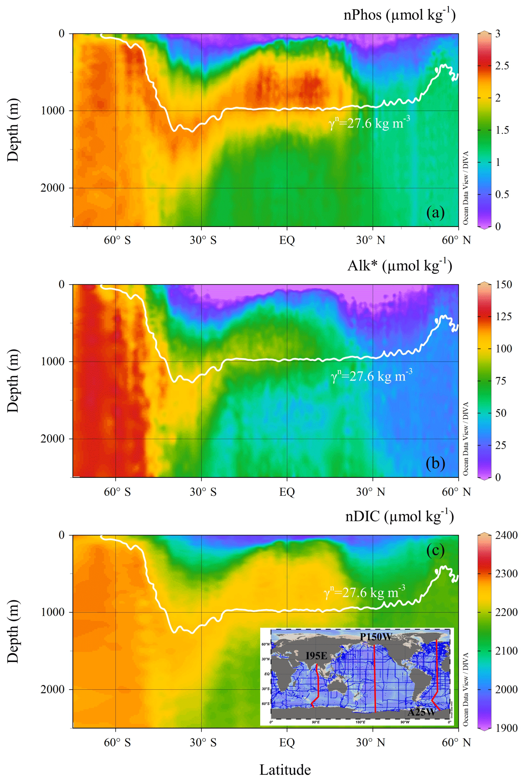
Figure 5Vertical distributions of (a) nPhos, (b) Alk∗, and (c) nDIC along the Atlantic Ocean section. The Indian and Pacific sections are not shown. The selected Atlantic section (A25W) is shown as the red line on the right-hand side of the inset. The neutral density isopycnal along which upwelling occurs is indicated by the white contour, which is characterized by neutral density of 27.6 kg m−3 in the Atlantic sector of the Southern Ocean.
Since nPhossurf tends to decrease to zero upon moving northwards, due to biological uptake, nDICsurf has a relatively constant value in the subtropical regions (data not shown), where it is not influenced by upwelling in the Southern Ocean. Because of this, the potential effect of upwelling on surface nDIC is calculated as the excess in nDICsurf compared to the subtropical average value (30∘ S–30∘ N):
2.5.3 Upwelled TA-driven effect (long-term effect of upwelling)
Some effects of upwelling on DIC are temporary, becoming overridden later by gas exchange. In contrast, the effect of upwelled TA persists because it changes the equilibrium DIC with respect to gas exchange (DICeq) (discussed also in Sect. 4.1.3). Upwelling of high-TA water has a long-lasting effect on DIC because, if all else remains constant, an increase in TA decreases the fraction of DIC that exists as CO2 molecules. The resulting decrease in CO2 concentration lowers seawater partial pressure of CO2 (pCO2), having the potential to lower seawater pCO2 to below atmospheric values which in turn drives an influx of CO2 from the atmosphere, raising DIC (Humphreys et al., 2017). The effects of upwelling are complex because they consist of both direct and indirect effects on DIC (Fig. 2), lasting over both short (when DIC is altered but DICeq is not) and long (when DICeq is altered) timescales. The different effects and the meanings of the terms used here are illustrated in Fig. 6.
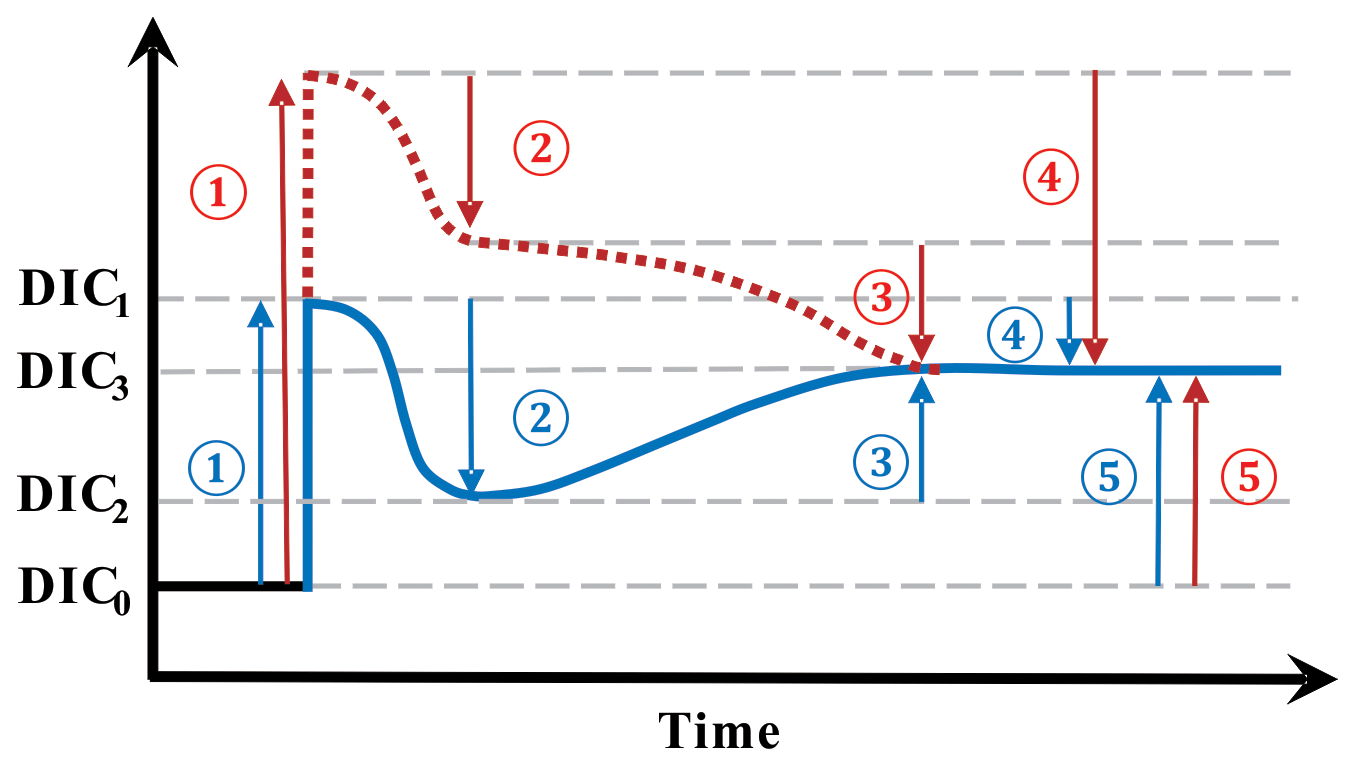
Figure 6A schematic illustrating the various effects of upwelling on surface DIC. Numbers represent processes changing surface DIC, and arrows point in the direction of change. (1) The direct effect of upwelling which elevates surface DIC from DIC0 to DIC1; (2) the DIC uptake by biology supported by upwelled nutrients, dropping DIC from DIC1 to DIC2. The processes of (1) and (2) make up the short-term effect of upwelling (i.e., difference between DIC2 and DIC0); (3) the change brought about by air–sea CO2 gas exchange which continues towards the equilibrium with the atmosphere (DIC3, whose level is determined by the amount of upwelled TA as well as by temperature); (4) the combination of both (2) and (3) makes up the total indirect effect of upwelling (the difference between DIC3 and DIC1); (5) the long-term impact of upwelling on the level of surface DIC is the difference between DIC3 and DIC0. Blue and red indicate two scenarios with different amounts of upwelled DIC relative to upwelled TA, but the same amounts of upwelled TA. Blue is for upwelled water with a deficit in additional DIC relative to additional TA whereas red is for an excess in DIC relative to TA.
The calculation of the long-term effect of upwelling through upwelled TA in the Southern Ocean (i.e., the difference between DIC3 and DIC0 in Fig. 6) was achieved through five steps.
-
Calculate TA in the Southern Ocean with the upwelling effect subtracted, TAnonupw:
where TAobs is the observed in situ TA, and Alk∗ is the TA tracer (Fry et al., 2015) revealing excess TA supplied by the large-scale ocean circulation (upwelling in the Southern Ocean), as well as removal by calcification and export (Eq. 12). Since Alk∗ is a salinity-normalized concept, it is necessary to restore it to the in situ salinity before subtracting it from the in situ TA.
-
Calculate in situ sea surface pCO2, following the same method as described in Sect. 2.5.1.
-
Calculate DIC with the effect of upwelled TA subtracted. We calculated DICnonupw using CO2SYS with inputs of TAnonupw and in situ pCO2, SST, and salinity.
-
Normalize salinity for consistency with other calculated effects.
-
Finally, the long-term effect of upwelling through the upwelled TA and the subsequent air–sea gas exchange is calculated as
where ΔnDICupw_lt corresponds to the magnitude of (5) in Fig. 6.
2.5.4 Iron-driven effect
The iron-limitation-driven DIC differences (ΔDICFe) relate to the concepts of “unused nutrient”, which can be thought of as the amounts of macronutrients and DIC that are left behind after iron limitation brings an end to biological uptake, in those regions where iron is the limiting nutrient. Iron limitation alters the impact of upwelling. In locations experiencing upwelling but where nitrate is the proximate limiting nutrient, the quantity of upwelled DIC might more or less be balanced by the quantity of subsequently exported DIC (fueled by the upwelled nutrients). In the Southern Ocean, however, the two appear not to be close to balance, even before considering iron limitation. According to the calculations in Sect. 2.5.2, the ratio of the excess upwelled nDIC against nPhos is around for the Southern Ocean, considerably exceeding the low C:P (average ) of organic matter in the region (Martiny et al., 2013). So even if all upwelled phosphate were to be used up and then exported in biomass in conjunction with carbon, a considerable surplus of DIC would be left behind. A lack of iron in surface waters, however, leads to even more upwelled DIC being left behind after the end of blooms induced by the upwelled nutrients.
We used phosphate as the unused nutrient from which to calculate ΔDICFe. For each grid in the surface open ocean, the unused phosphate was taken from its annual minimum concentration based on the monthly data in World Ocean Atlas 2013 version 2 (WOA, 2013: https://www.nodc.noaa.gov/OC5/woa13/, last access: 30 January 2019, Boyer et al., 2013; Garcia et al., 2014). The unused phosphate was then converted into unused DIC based on a standard RC:P of 106:1 (Redfield, 1963) for most of the global ocean, with the exceptions described in Sect. 2.5.2.
The amount of ΔDICFe was therefore calculated as
2.6 Uncertainty estimation
Uncertainties in the effects of different drivers were determined by a Monte Carlo approach (following, e.g., Juranek et al., 2009; Ribas-Ribas et al., 2014). For example, the uncertainty of ΔnDICtemp was calculated as follows: (1) given that ΔnDICtemp is the difference between nDICobs and nDICSST=27 (Eq. 9), its uncertainty is propagated from the uncertainties of both nDICobs and nDICSST=27, where the uncertainty of nDICobs is 5 µmol kg−1 (Table 2), and the uncertainty of nDICSST=27 was determined by a Monte Carlo approach; (2) for calculation of the uncertainty of nDICSST=27 (see its function in Table 1), we first calculated artificial random errors (normally distributed according to the central limit theorem, with a mean of zero and a standard deviation equal to the accuracy/uncertainty of measurement) using a random number generator. Then, new carbonate system variable values (the original ones plus the randomly generated errors) were input into the CO2SYS program (van Heuven et al., 2011) to calculate new nDICSST=27 values. By doing this 1000 times, we obtained a set of 1000 different values for every single data point in the dataset. We used the standard deviations of these sets to characterize their individual uncertainties. The overall uncertainty of nDICSST=27 was 6.4 µmol kg−1; (3) by applying the same Monte Carlo method, but to calculate the uncertainty propagated through Eq. (9), we then calculated the uncertainty of ΔnDICtemp to be 8.0 µmol kg−1 (see Table 2 for other variables).
Table 2Uncertainties for variables in this study.
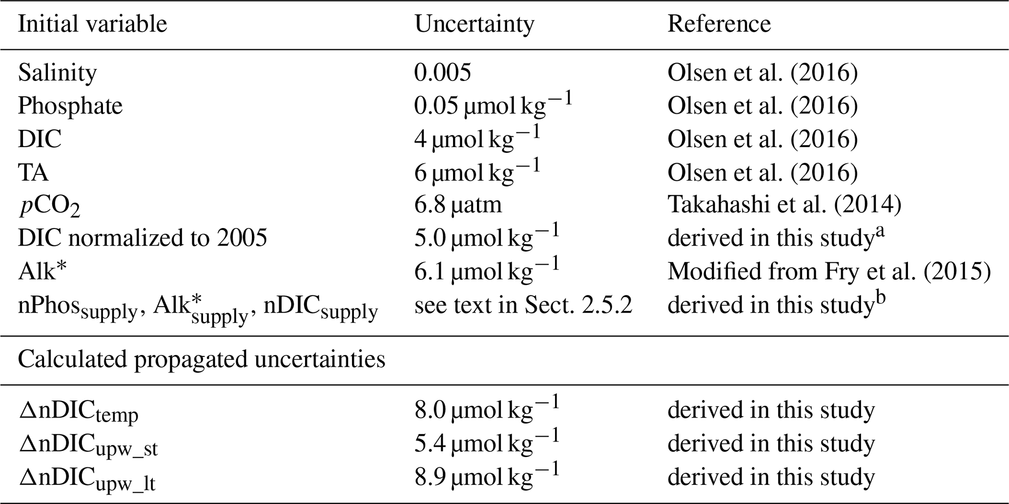
a The uncertainty of DIC normalized to 2005 was primarily propagated from TA and . The uncertainty of was calculated from error propagation (Fornasini, 2008) to be 0.17 µatm. b The uncertainties for variables with the subscript “supply” were from their standard error of the mean.
3.1 Spatial distributions of observed DIC and nDIC
Surface observations reveal values of DIC across the global ocean ranging from less than 1850 µmol kg−1 in the tropics to more than 2200 µmol kg−1 in the high latitudes (Fig. 1a). To first order, surface DIC increases polewards, being positively correlated with absolute latitude (Spearman's rank correlation coefficient ρ=0.71 for the global oceans, Table 3). Spatially, it is monotonically inversely related to sea surface temperature (, Table 3), with DIC being highest where the surface ocean is coolest. Another conspicuous feature of surface DIC is the higher values (by ∼100 µmol kg−1) in the tropical and subtropical Atlantic Ocean relative to the same latitudes in the Pacific and Indian oceans (Fig. 1a), as attributed to the transport of water vapor from the Atlantic to the Pacific (Broecker, 1989). This is not considered further here because our main purpose is to explain the sizable observed latitudinal gradients in DIC (on average 153 µmol kg−1 higher in the Southern Ocean than at low latitudes, for instance) and nDIC (on average 223 µmol kg−1 higher in the Southern Ocean than at low latitudes).
Table 3Global and regional correlations between DIC and nDIC and SST and latitude.
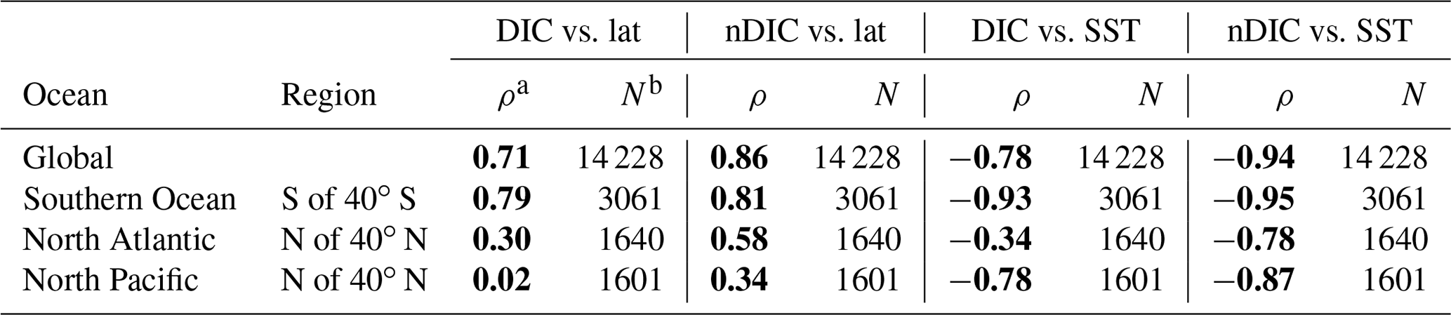
a The Spearman's rank correlation coefficient, for assessing monotonic relationships (there is a nonlinear relationship between SST and CO2 solubility). Statistically significant correlations are shown in bold. b The number of data points from that area that were used in calculating the correlations.
Salinity-normalized DIC (nDIC) increases towards the poles in all three ocean basins (Fig. 1b), although less strongly in the North Atlantic. The surface nDIC correlates more tightly with latitude and SST than does DIC, yielding a positive correlation with absolute latitude and a negative correlation with SST (ρ=0.86 and −0.94, respectively, for the global ocean, Table 3).
The distributions of surface DIC and particularly nDIC also show modest regional maxima in the eastern equatorial Pacific, the Arabian Sea, and the eastern boundaries of the Pacific and Atlantic ocean basins, presumably as a result of upwelling (Capone and Hutchins, 2013; Chavez and Messié, 2009; Millero et al., 1998; Murray et al., 1994).
3.2 SST-driven effect in the global surface ocean
The differences between the latitudinal patterns of DICobs and DICSST=27 are shown in Fig. 7. As expected, DICSST=27 agrees well with DICobs in the subtropics where SST is close to 27 ∘C; the differences become larger with increasing latitude and decreasing SST (Fig. 7a–c). Correcting for salinity variations (Fig. 7d–f) greatly reduces the variability in DIC at low latitudes: nDICobs is fairly constant at ∼1970 µmol kg−1 in the subtropics. ΔnDICtemp (Eq. 8 but for nDIC), the temperature-driven CO2 gas exchange effect on surface nDIC, increases sharply with latitude (Fig. 7g–i), reaching ∼200 µmol kg−1 at 60∘ N in the northern part of the Atlantic and Pacific oceans and ∼220 µmol kg−1 at 70∘ S in the Southern Ocean. The average ΔnDICtemp in the Southern Ocean is 182 µmol kg−1, which is large enough to account by itself for most – but not all – of the nDIC latitudinal gradient of 223 µmol kg−1 (2193–1970 µmol kg−1).

Figure 7Latitudinal distributions of calculated temperature effect on surface DIC. Different columns show different basins (Atlantic, Indian, and Pacific) and different rows show different calculated DIC variables. Panels (a), (b), and (c) show the observed surface DIC (black) and predicted DIC at SST of 27 ∘C (red). Panels (d), (e), and (f) show the observed surface nDIC (black) and predicted nDIC at SST of 27 ∘C (red). Panels (g), (h), and (i) show ΔnDICtemp, where nDICSST=27 is subtracted from nDICobs to obtain the calculated temperature effect.
ΔDICtemp and ΔnDICtemp are very similar in magnitude, with the largest deviations (at high latitudes) being less than 10 µmol kg−1. Uncertainties associated with the salinity normalization process must therefore be small and are not considered further.
The estimated overall uncertainty of the SST-driven effect on surface nDIC (Table 2) ranges from 5 to 8 µmol kg−1, which is of comparable magnitude to the uncertainty of DIC normalized to 2005 and much smaller than the large latitudinal variations in ΔnDICtemp.
3.3 Upwelling-driven effects in the Southern Ocean
The upwelling-driven effects in the Southern Ocean calculated from both short- and long-term perspectives are shown in Fig. 8. The values were calculated from data collected along selected transects in each of the Atlantic, Indian, and Pacific sectors.
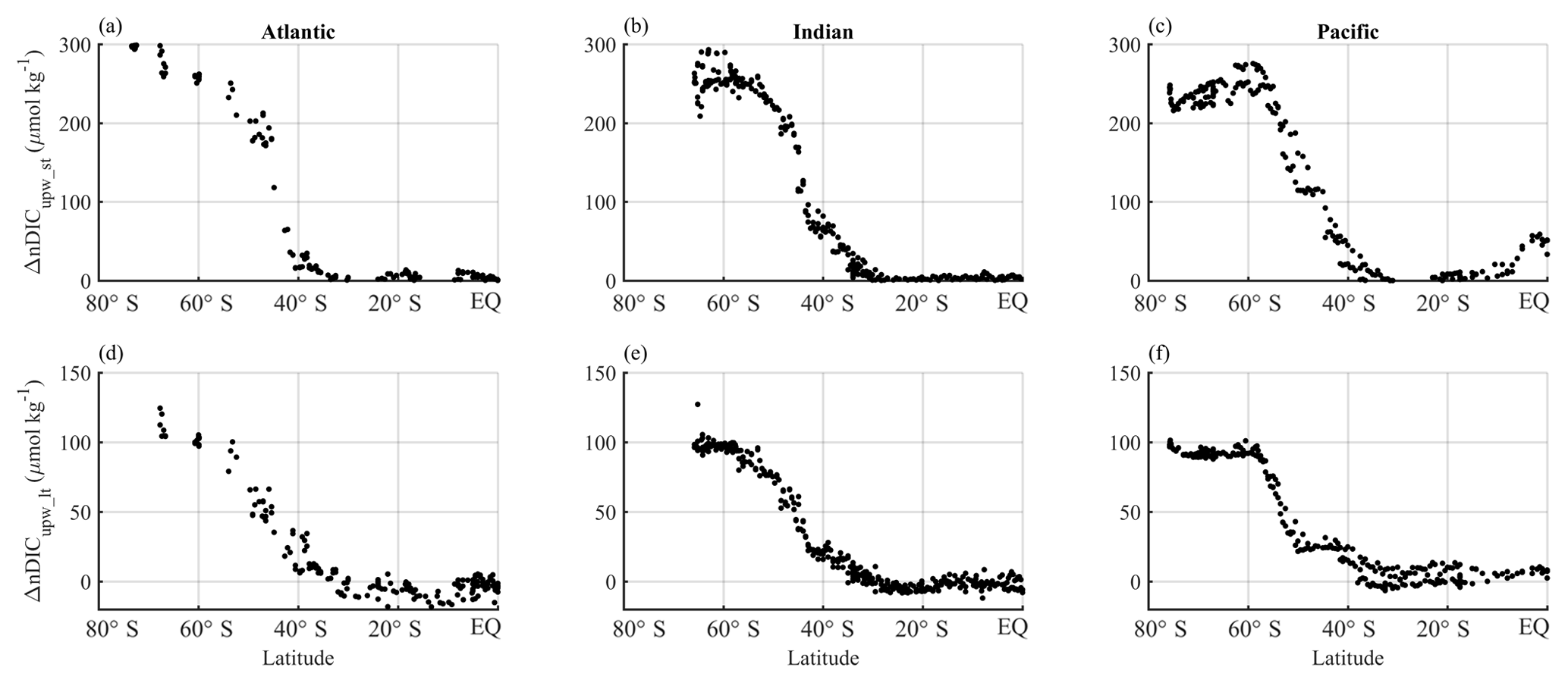
Figure 8Latitudinal distributions of calculated upwelling effects on surface nDIC. Different columns show different sectors in ocean basins (Atlantic, Indian, and Pacific) and different rows show different calculated effects on surface DIC. Panels (a), (b), and (c) show the short-term effect of upwelling (ΔnDICupw_st), which is driven by the direct supply of DIC from deep water and subsequent change by biology in the Southern Ocean. Panels (d), (e), and (f) show the long-term effect of upwelling (ΔnDICupw_lt), which is the difference between the observed nDIC value (determined mainly by the amount of upwelled TA, as well as by SST) and pre-upwelling nDIC value. The results were calculated from the three selected transects defined in Sect. 2.5.2.
ΔnDICupw_st increases polewards (Fig. 8a–c), with the same trends as surface phosphate (not shown), because it is calculated from phosphate. It can be seen that surface nDIC is potentially elevated dramatically by the Southern Ocean upwelling. The effect is of larger magnitude (average of 220 µmol kg−1 in the Southern Ocean) than that calculated for ΔnDICtemp (Fig. 7g–i).
Figure 8d–f show the long-term effect of upwelling, which is controlled by the concentration of TA in the upwelled water (how much upwelling increases surface TA values by). The average magnitude of ΔnDICupw_lt is around 74 µmol kg−1 for the Southern Ocean.
The estimated overall uncertainty of upwelling-driven effects on surface nDIC (Table 2) ranges from 5 to 9 µmol kg−1, close to the uncertainty of DIC normalized to 2005, and much smaller than the large latitudinal variations in ΔnDICupw_st and ΔnDICupw_lt.
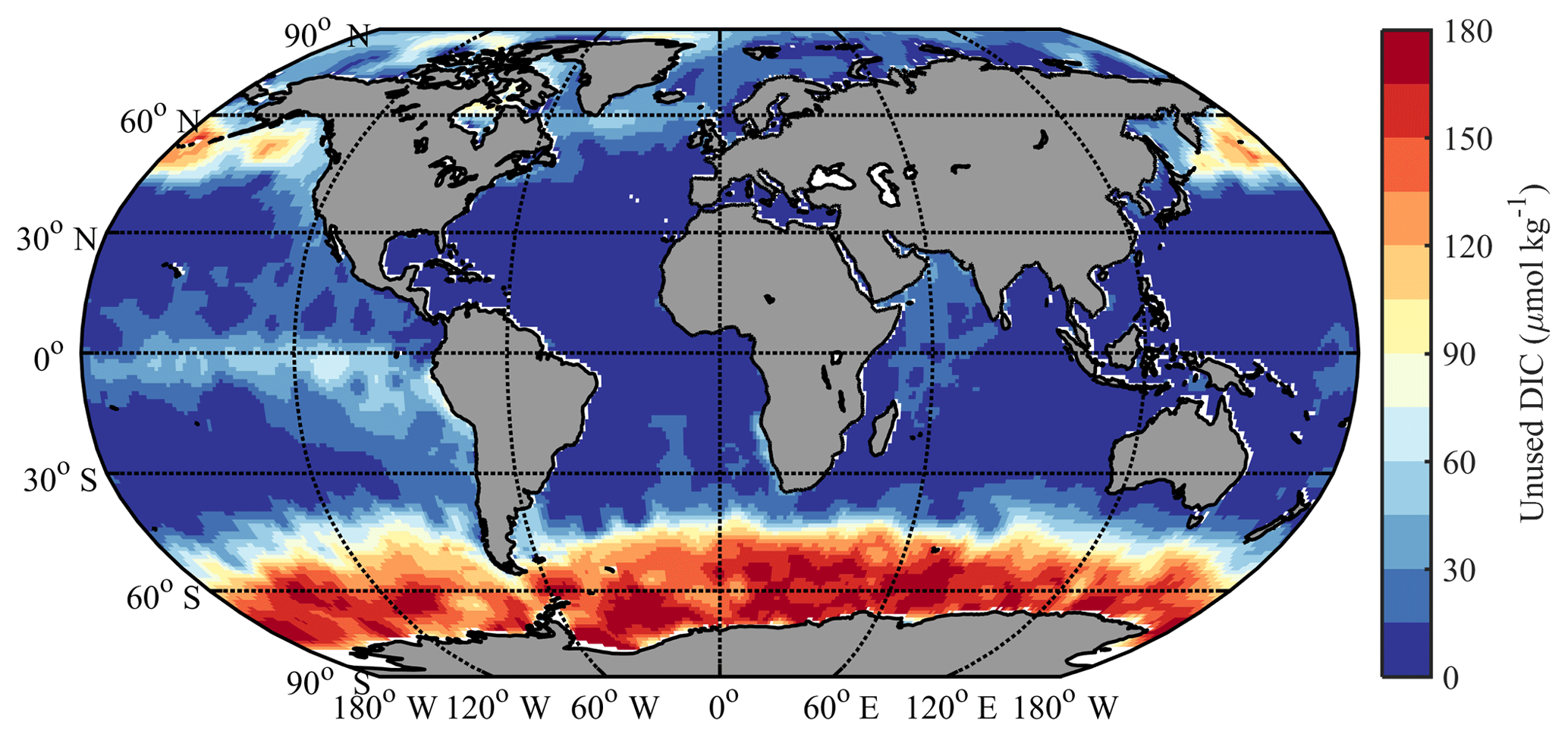
Figure 9Calculated potential impact of iron limitation on surface DIC. Different colors correspond to different amounts of “unused DIC”, calculated with the Redfield ratio from observed residual phosphate.
3.4 Iron-driven effect in the global surface ocean
As shown in Fig. 9, ΔDICFe is close to zero except in the classic HNLC regions (i.e., the North Pacific, the equatorial Pacific, and the Southern Ocean; Moore et al., 2013). There is also some residual nitrate during most summers in the Iceland and Irminger basins of the North Atlantic due to the seasonal iron limitation there (Nielsdóttir et al., 2009). The surface Southern Ocean south of 40∘ S has the largest unused DIC (ΔDICFe of up to 180 µmol kg−1, average of 120 µmol kg−1), followed by the North Pacific 40–65∘ N (ΔDICFe of up to 120 µmol kg−1, average of 75 µmol kg−1) and the equatorial Pacific (average of 35 µmol kg−1). It is negligible elsewhere in the tropics and subtropics.
4.1 Factors controlling the surface nDIC latitudinal variation
All effects discussed in this section are effects on nDIC rather than on DIC.
4.1.1 Effect of SST variation in the global surface ocean
The previously accepted explanation for higher DIC at high latitudes is that cooler SSTs there increase CO2 solubility, resulting in a higher equilibrium DIC (Toggweiler et al., 2003a; Williams and Follows, 2011). Our results support an important role for SST, but also that other processes contribute significantly.
Our analysis concludes that the latitudinal gradient in temperature is capable of raising nDIC by about 180 µmol kg−1 in the Southern Ocean, or in other words, explaining about four-fifths of the observed gradient of 223 µmol kg−1. SST variation is thus able to explain most of the observed pattern.
4.1.2 Effect of TA distribution in the global surface ocean
A second factor that has been proposed as influential in driving spatial variations in the concentration of DIC in the surface ocean is TA (Williams and Follows, 2011). Our analysis supports this conclusion, although we note that the effect of TA is most prominent at low latitudes. Large differences in DIC are observed between the subtropical gyres, where values are relatively high, and the vicinity of the Equator, where values are relatively low (Fig. 1a). These differences in DIC are driven initially by the direct effects of evaporation and precipitation on DIC. However, direct effects of evaporation and precipitation on TA also lead to indirect effects on DIC because of the influence of TA on the value of DIC required for gas exchange equilibrium with a given atmospheric CO2 level. The indirect effects will dominate over longer timescales (see Sect. 4.2 and Fig. 6). The role of TA explains the much clearer relationship between latitude and nDIC than between latitude and DIC (Fig. 1, Table 3); normalizing DIC to salinity is almost the same as normalizing DIC to TA because salinity and TA are highly correlated in the surface open ocean. As a result, the effect of TA on DIC is counteracted by salinity normalization, with the pattern in nDIC (Fig. 1b) then revealing more clearly how other factors impact DIC.
The latitudinal pattern in TA is not the dominant driver of the DIC trend because TA values are generally lower at high latitudes (where precipitation often exceeds evaporation) than they are at low latitudes (where evaporation often exceeds precipitation). However, TA is also biologically cycled and thus not perfectly correlated to salinity (Fry et al., 2015) and the presence of excess TA in deep water upwelled at high latitudes does contribute to the DIC trend.
4.1.3 Effect of upwelling in the Southern Ocean
Although not traditionally considered a factor, our analyses show that upwelling is important in driving the latitudinal gradient in DIC. Upwelling of DIC by itself is capable of producing an nDIC latitudinal gradient of 220 µmol kg−1 in the Southern Ocean, even higher than the effect of temperature (Fig. 8a–c, Table 4). However, the contribution of upwelling is reduced by about two-thirds if only the long-term effect through upwelled TA is considered (see Fig. 6 for definitions of terms).
Table 4Summary of nDIC differences between low and high latitudes. Each ΔnDIC value is the amount by which the annual average nDIC value for the high-latitude region exceeds the annual average value for the low latitudes (30∘ S to 30∘ N). Percentages in brackets represent the proportion of the observed nDIC difference in the second column; n.c.: not calculated.
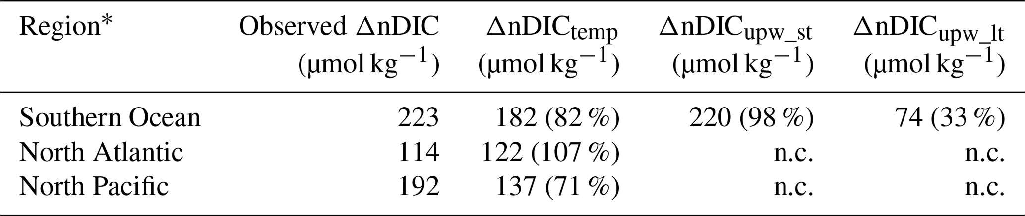
* The regions are defined as follows: North Atlantic: 40–60∘ N; North Pacific: 40–60∘ N; Southern Ocean: south of 40∘ S.
Deep water usually has higher concentrations of nutrients, nDIC and nTA, than surface water does. Introduction of deep water into the surface mixed layer therefore usually stimulates increases in these concentrations, with three main consequences for DIC (Fig. 6) as follows. (a) If the upwelled water has higher DIC than the surface, the upwelling causes an immediate initial increase in DIC; (b) additional nutrients stimulate phytoplankton blooms until the proximate limiting nutrient runs out, leading to a reduction in DIC over timescales of days to weeks (or months if, for instance, the upwelling occurs at high latitudes during winter when phytoplankton cannot bloom); (c) finally, air–sea gas exchange tends to remove any upwelling-induced air–sea CO2 disequilibrium over a period of months to a year (Jones et al., 2014), although full equilibrium is seldom achieved across the global surface ocean (Takahashi et al., 2014).
The upwelling effects in Fig. 8 are calculations based on phosphate and TA concentrations, taking into account both the amount upwelled and the amount subsequently removed by biology. They therefore correspond to the sum of the direct upwelling effect (1 in Fig. 6) and the indirect upwelling effect through supplied nutrients (2 in Fig. 6). There are two reasons why the initial amount of upwelled DIC considerably exceeds the amount of DIC subsequently taken up by phytoplankton growth fueled by the upwelled nutrients (why 1 > 2) in the Southern Ocean.
Firstly, iron is typically much scarcer in deep waters than macronutrients are, relative to phytoplankton need (Moore, 2016). Regions like the Southern Ocean that are strongly influenced by upwelling are for this reason often iron-limited (Moore, 2016), leading to large amounts of “unused DIC” (order of 120 µmol kg−1 in the Southern Ocean – Fig. 9) accompanying unused macronutrients. This scarcity of iron also leads to muted seasonal cycles of DIC (Merlivat et al., 2015) and thus year-round persistence of unused DIC. Secondly, as described in Sect. 2.5.2, the higher C:P ratio of supply () compared to removal () implies a considerable surplus of DIC even without iron limitation.
The upwelling effects shown in Fig. 8a–c are however relatively short term, and are expected to be overridden by air–sea gas exchange within months (Jones et al., 2014). They are thus likely to be most significant in the vicinity of where upwelling takes place (Morrison et al., 2015). For effects that may persist further away from locations of upwelling, it is important to also consider the long-term effect (5 in Fig. 6), the magnitude of which is dictated mainly by the change in TA brought about by upwelling. The level of TA in upwelled water (∼2315, 2340, and 2337 µmol kg−1 in the Atlantic, Indian, and Pacific sectors of the Southern Ocean, respectively, calculated according to the same method as in Sect. 2.5.2) are higher than the typical levels of TA in the surface waters of the high-latitude Southern Ocean (∼2300, 2289, and 2288 µmol kg−1 in the Atlantic, Indian, and Pacific sectors, respectively). The increase in TA brought about by upwelling corresponds to a long-term upwelling effect on nDIC of about 74 µmol kg−1 (Fig. 8d–f) in the Southern Ocean.
Our results show that upwelling in the Southern Ocean can, by itself, generate high-latitude nDIC values that are around 220 µmol kg−1 greater than subtropical values. We emphasize that there is also a sizable long-term effect of upwelling (forcing nDIC values to be around 74 µmol kg−1 higher than they would be otherwise) after the operation of short-term effect. Contrary to what might typically be assumed, the long-term effects of upwelling are dictated by the amounts of TA upwelled, and not by the amounts of DIC or nutrients.
4.2 A new understanding of the controls on the surface DIC distribution
Our analysis revises the prevailing paradigm of the causes of the latitudinal gradient in surface DIC. Previously, the gradient was thought to be completely explained by the effect of sea surface temperature on CO2 solubility, but we have shown that upwelling is also an important contributor. DIC and nDIC would still be elevated at high latitudes even without any temperature effect.
Neither temperature patterns nor upwelling are responsible for all of the observed large latitudinal gradients in DIC and nDIC (for instance, the ∼220 µmol kg−1 difference in nDIC between low latitudes and the Southern Ocean), but rather they are jointly responsible. There is an apparent contradiction because both ΔnDICtemp and ΔnDICupw_st appear to account for more than 80 % of the nDIC latitudinal gradient. While both processes are capable individually of raising nDIC by 182 and 220 µmol kg−1 in the Southern Ocean, acting together they raise it by only 223 µmol kg−1 instead of 400 µmol kg−1. An obvious explanation of this apparent paradox is that when we consider upwelling effects, we should consider not only its short-term effect through supplying DIC and nutrients (1+2 in Fig. 6), but also its long-term effect with gas exchange with the atmosphere ( in Fig. 6), the amount of which is a function of the amount of upwelled TA (which, together with temperature, controls the equilibrium DIC). The sum of the SST-driven effect and the long-term effect of upwelling approximately equals the nDIC latitudinal gradient (Table 4).
On the global scale, therefore, the ultimate controls on the surface DIC and nDIC latitudinal gradients are the spatial patterns of SST and upwelling, and the chemical composition of the upwelled water.
4.3 Importance of upwelling confirmed by the North Atlantic
From inspection of the global nDIC distribution (Fig. 1b), it can be seen that nDIC increases with latitude in all basins, but, as shown in Table 4, does so less strongly in the North Atlantic (difference between high latitudes and low latitudes of 114 µmol kg−1) than in the North Pacific (difference of 192 µmol kg−1). Although the latitudinal temperature gradient is less pronounced in the North Atlantic, this is not enough to explain the variation in gradients between the two basins: the average temperature of the high-latitude North Atlantic is 12.4 ∘C and of the high-latitude North Pacific is 9.5 ∘C, which can explain about 20 µmol kg−1 of variation between the two nDIC gradients but cannot explain the observed 78 µmol kg−1 variation (Table 4).
The reason for the discrepancy is that the Southern Ocean and the North Pacific experience elevations in values due to inputs of deep water whereas the North Atlantic does not. Upwelling occurs in the Southern Ocean and entrainment due to deep winter mixing occurs in the subarctic North Pacific (Mecking et al., 2008; Ohno et al., 2009) where it entrains waters high in both TA (Fry et al., 2016) and DIC. While deep winter mixing also occurs in the high-latitude North Atlantic (de Boyer Montégut et al., 2004), the entrained waters left the surface relatively recently and hence there is little accumulated remineralized DIC and TA in the deep water that is reintroduced to the surface. For this reason, winter entrainment produces little increase in surface nDIC in the North Atlantic. This makes the North Atlantic useful in discriminating between the two effects because, uniquely out of the three regions, only the SST effect operates there. As expected, the SST effect is able to completely account for the observed nDIC gradient in the North Atlantic, whereas it cannot in the other two regions (second and third columns in Table 4). The North Atlantic confirms the important contribution of upwelling to latitudinal gradients, while also showing that latitudinal gradients occur in the absence of upwelling.
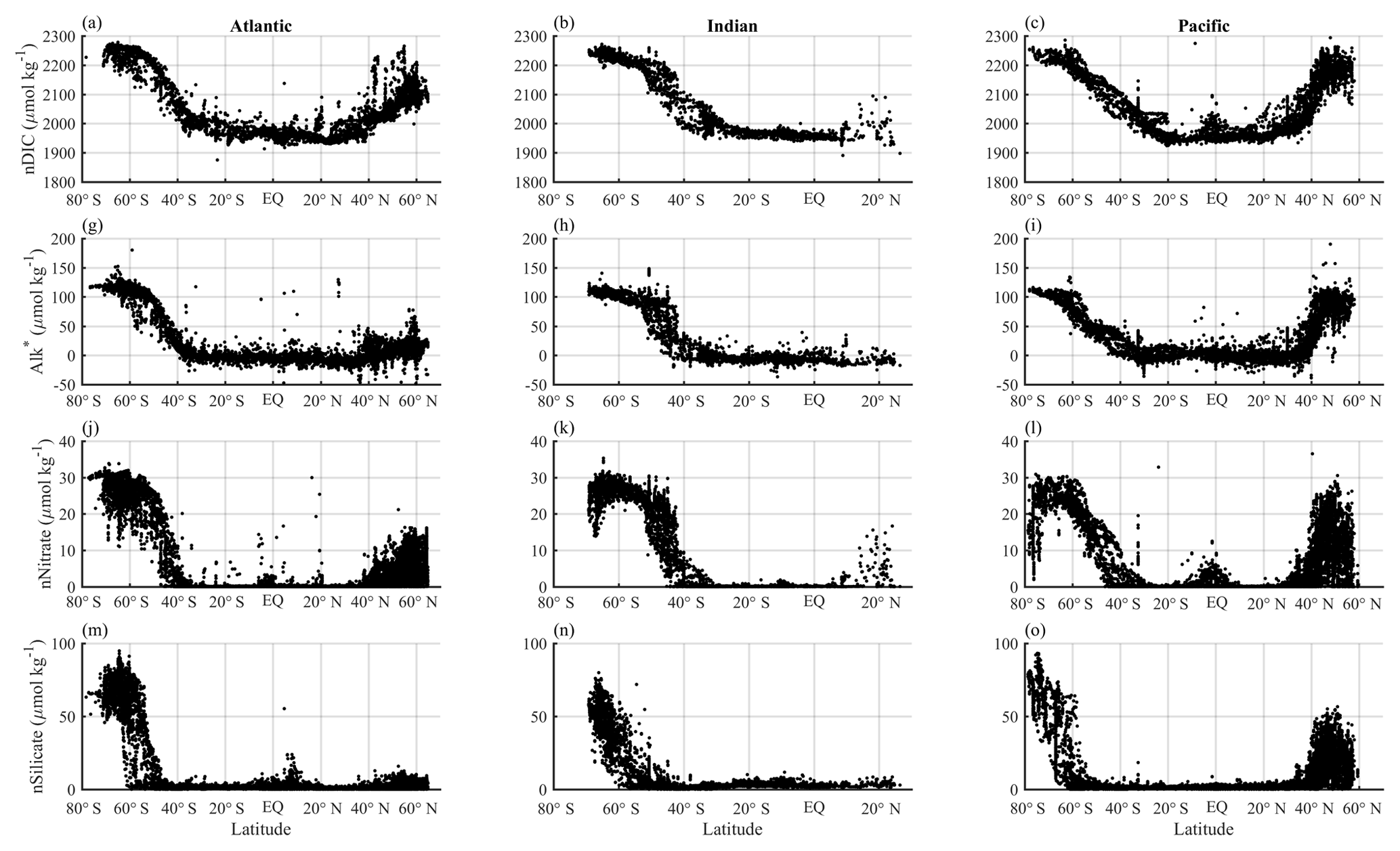
Figure 10Latitudinal distributions of sea surface nDIC, Alk∗ (Fry et al., 2015), salinity-normalized nitrate, and silicate in each ocean basin.
4.4 Comparison of nDIC distribution to Alk∗ and nutrients
Figure 10 shows a comparison between the patterns of nDIC, the TA tracer Alk∗ (Eq. 11; Fry et al., 2015), and salinity-normalized nutrients. The similarities and differences in distributions of Alk∗ and nutrients have previously been discussed by Fry et al. (2015). Here we extend the comparison to also include nDIC. All exhibit low and fairly constant values at low latitudes. This is primarily due to biological uptake and restricted supply from subsurface waters, for most variables, but is also due to fairly uniform high temperatures for nDIC. All increase polewards due to upwelling/entrainment (and also declining SST for nDIC), and all exhibit maxima at high latitudes in the Southern Ocean and North Pacific. All exhibit a more modest increase in the North Atlantic than in the North Pacific because the deep water formed relatively recently. There are differences in the latitudes at which the different parameters start to increase when moving from the Equator towards Antarctica, reflecting the different processes involved. Surface nDIC is the first to start increasing, under the influence of SST (third row in Fig. 7), at 20–25∘ S. Alk∗ and nutrients, however, influenced by upwelling/entrainment, do not start to increase until somewhere between 30 and 50∘ S.
4.5 Implications for the future CO2 sink under climate change
It is widely understood that global warming may alter the spatial distribution and intensity of upwelling in the ocean (Bakun, 1990; McGregor et al., 2007; Wang et al., 2015). It could either increase it on average, due to higher average wind speeds in a warmer, more energetic atmosphere (Bakun, 1990; Wang et al., 2015), or decrease it on average, due to enhanced stratification as the temperature differential between surface and deep waters is increased (Barton et al., 2013; Sarmiento et al., 2004). Furthermore, it is widely understood that an increase in upwelling would lead to an increase in the amount of CO2 outgassed from the ocean, as larger quantities of CO2-rich deep water are brought up to the surface and their CO2 vented to the atmosphere (Evans et al., 2015; Marinov et al., 2006; Morrison et al., 2015). However, we have identified an additional effect here. Changes in upwelling would alter the distribution of carbon in the surface ocean not only through the supply of CO2, but also through the supply of TA, which determines the eventual surface carbonate system equilibrium with the same atmospheric pCO2 (Humphreys et al., 2018). That is to say, the impact of changes in upwelling on the ocean's carbon source–sink strength depends not only on the DIC content of the upwelled water but also on its TA content. Ocean carbon cycle models should include these additional consequences if they are to make accurate predictions about the impacts of global warming on future carbon cycling. They should include the several routes identified here by which upwelling affects surface DIC: through upwelling of DIC, through upwelling of nutrients, and through upwelling of TA.
We investigated the global surface DIC and nDIC distributions in order to explain the large differences between high-latitude (especially Southern Ocean) and low-latitude regions. This issue has been addressed in previous studies and here we revisited it using new analytical approaches that lead to new findings. We considered three drivers for how the phenomenon could be explained: (1) sea surface temperature variations through their effect on CO2 system equilibrium constants, (2) salinity-related TA variations through their effect on pCO2, and (3) upwelling in the subpolar oceans. Our analyses confirmed that temperature plays a dominant role through its effect on solubility, and is able to explain a large fraction of the surface nDIC latitudinal gradient (182 µmol kg−1 out of 223 µmol kg−1 in the high-latitude Southern Ocean). Variations in TA associated with evaporation and precipitation are unable to explain higher DIC concentrations at higher latitudes because alone they would drive the opposite DIC pattern. Their role is therefore to reduce the magnitude of the polewards gradient in DIC. Upwelling, whose role in driving the large-scale spatial patterns has not previously been appreciated, accounts for a sizable component of the surface nDIC latitudinal gradient (on average 220 µmol kg−1 in the Southern Ocean). Its importance is magnified by the iron limitation that frequently occurs in upwelling areas, leaving behind residual upwelled excess DIC and macronutrients that cannot be utilized by biology. We emphasize that the upwelling of TA alongside DIC generates a prolonged effect that persists beyond CO2 gas exchange re-equilibration timescales. The long-term effect of upwelling (74 µmol kg−1 in the Southern Ocean) helps explain the shortfall between the observed nDIC latitudinal gradient (223 µmol kg−1) and the magnitude of the temperature-driven effect (182 µmol kg−1). On the global scale, we conclude that no single mechanism accounts for the full amplitude of surface DIC latitudinal variations but that temperature and the long-term effect of upwelling, in that order, are the two major drivers.
Data for this study came from the Global Ocean Data Analysis Project version 2 (GLODAPv2, Key et al., 2015; Olsen et al., 2016). All the data used is publicly available at the Ocean Carbon Data System (OCADS, https://www.nodc.noaa.gov/archive/arc0107/0162565/2.2/data/0-data/data_product/).
YW and TT developed the theoretical formalism and conceived the original idea. YW performed the analytic calculations and the computational framework. TT supervised the project. YW and TT wrote the paper, with all authors discussing the results, providing suggestions for further analysis, and commenting on the paper.
The authors declare that they have no conflict of interest.
We thank Nicolas Metzl from the French National Centre for Scientific Research for providing the corrections for TA and DIC data for the KERFIX time-series station (which was included but not corrected as part of GLODAPv2). The suggested corrections for KERFIX were TA by −49 µmol kg−1 and DIC by −35 µmol kg−1 (Jouandet et al., 2008; Metzl et al., 2006). We thank the three anonymous reviewers for their careful reviews.
This research has been supported by the Swire Educational Trust and RAGNARoCC (grant no. NE/K002546/1).
This paper was edited by Jack Middelburg and reviewed by three anonymous referees.
Bakun, A.: Global climate change and intensification of coastal ocean upwelling, Science, 247, 198–201, https://doi.org/10.1126/science.247.4939.198, 1990.
Balch, W. M., Bates, N. R., Lam, P. J., Twining, B. S., Rosengard, S. Z., Bowler, B. C., Drapeau, D. T., Garley, R., Lubelczyk, L. C., Mitchell, C., and Rauschenberg, S.: Factors regulating the Great Calcite Belt in the Southern Ocean and its biogeochemical significance, Global Biogeochem. Cy., 30, 1124–1144, https://doi.org/10.1002/2016GB005414, 2016.
Barton, E. D., Field, D. B., and Roy, C.: Canary current upwelling: More or less?, Prog. Oceanogr., 116, 167–178, https://doi.org/10.1016/j.pocean.2013.07.007, 2013.
Bates, N., Astor, Y., Church, M., Currie, K., Dore, J., Gonaález-Dávila, M., Lorenzoni, L., Muller-Karger, F., Olafsson, J., and Santa-Casiano, M.: A time-series view of changing ocean chemistry due to ocean uptake of anthropogenic CO2 and ocean acidification, Oceanography, 27, 126–141, 2014.
Bates, N. R., Michaels, A. F., and Knap, A. H.: Seasonal and interannual variability of oceanic carbon dioxide species at the US JGOFS Bermuda Atlantic Time-series Study (BATS) site, Deep-Sea Res. Pt. II, 43, 347–383, https://doi.org/10.1016/0967-0645(95)00093-3, 1996.
Bates, N. R., Pequignet, A. C., and Sabine, C. L.: Ocean carbon cycling in the Indian Ocean: 1. Spatiotemporal variability of inorganic carbon and air-sea CO2 gas exchange, Global Biogeochem. Cy., 20, GB3020, https://doi.org/10.1029/2005GB002491, 2006.
Boyer, T. P., Antonov, J. I., Baranova, O. K., Coleman, C., Garcia, H. E., Grodsky, A., Johnson, D. R., Locarnini, R. A., Mishonov, A. V., O'Brien, T. D., Paver, C. R., Reagan, J. R., Seidov, D., Smolyar, I. V., and Zweng, M. M.: World Ocean Database 2013, NOAA Atlas NESDIS 72, edited by: Levitus, S., Technical edited by: Mishonov, A., Silver Spring, MD, 209 pp., https://doi.org/10.7289/V5NZ85MT, 2013.
Bozec, Y., Thomas, H., Schiettecatte, L. S., Borges, A. V., Elkalay, K., and de Baar, H. J. W.: Assessment of the processes controlling seasonal variations of dissolved inorganic carbon in the North Sea, Limnol. Oceanogr., 51, 2746–2762, 2006.
Brewer, P. G. and Goldman, J. C.: Alkalinity changes generated by photoplankton growth, Limnol. Oceanogr., 21, 108–117, 1976.
Broecker, W. S.: The salinity contrast between the Atlantic and Pacific oceans during glacial time, Paleoceanography, 4, 207–212, https://doi.org/10.1029/PA004i002p00207, 1989.
Cai, W. J., Hu, X., Huang, W. J., Jiang, L. Q., Wang, Y., Peng, T. H., and Zhang, X.: Alkalinity distribution in the western North Atlantic Ocean margins, J. Geophys. Res.-Oceans, 115, C08014, https://doi.org/10.1029/2009JC005482, 2010.
Cameron, D. R., Lenton, T. M., Ridgwell, A. J., Shepherd, J. G., Marsh, R., and Yool, A.: A factorial analysis of the marine carbon cycle and ocean circulation controls on atmospheric CO2, Global Biogeochem. Cy., 19, GB4027, https://doi.org/10.1029/2005GB002489, 2005.
Capone, D. G. and Hutchins, D. A.: Microbial biogeochemistry of coastal upwelling regimes in a changing ocean, Nat. Geosci., 6, 711–717, https://doi.org/10.1038/ngeo1916, 2013.
Chavez, F. P. and Messié, M.: A comparison of eastern boundary upwelling ecosystems, Prog. Oceanogr., 83, 80–96, https://doi.org/10.1016/j.pocean.2009.07.032, 2009.
Clargo, N. M., Salt, L. A., Thomas, H., and de Baar, H. J. W.: Rapid increase of observed DIC and pCO2 in the surface waters of the North Sea in the 2001–2011 decade ascribed to climate change superimposed by biological processes, Mar. Chem., 177, 566–581, https://doi.org/10.1016/j.marchem.2015.08.010, 2015.
de Boyer Montégut, C., Madec, G., Fischer, A. S., Lazar, A., and Iudicone, D.: Mixed layer depth over the global ocean: An examination of profile data and a profile-based climatology, J. Geophys. Res.-Ocean., 109, C12003, https://doi.org/10.1029/2004JC002378, 2004.
Dickson, A. G.: Standard potential of the reaction: AgCl(s) + 12H2(g) = Ag(s) + HCl(aq), and and the standard acidity constant of the ion HSO in synthetic sea water from 273.15 to 318.15 K, J. Chem. Thermodyn., 22, 113–127, 1990.
Dickson, A. G. and Millero, F. J.: A comparison of the equilibrium constants for the dissociation of carbonic acid in seawater media, Deep-Sea Res., 34, 1733–1743, 1987.
Doney, S. C., Fabry, V. J., Feely, R. A., and Kleypas, J. A.: Ocean acidification: the other CO2 problem, Ann. Rev. Mar. Sci., 1, 169–192, https://doi.org/10.1146/annurev.marine.010908.163834, 2009.
Evans, W., Hales, B., Strutton, P. G., Shearman, R. K., and Barth, J. A.: Failure to bloom: Intense upwelling results in negligible phytoplankton response and prolonged CO2 outgassing over the Oregon shelf, J. Geophys. Res.-Ocean., 120, 1446–1461, https://doi.org/10.1002/2014JC010580, 2015.
Falkowski, P. G., Scholes, R. J., Boyle, E., Canadell, J., Canfield, D., Elser, J., Gruber, N., Hibbard, K., Högberg, P., Linder, S., Mackenzie, F. T., Moore III, B., Pedersen, T., Rosenthal, Y., Seitzinger, S., Smetacek, V., and Steffen, W.: The global carbon cycle: a test of our knowledge of Earth as a system, Science, 290, 291–296, https://doi.org/10.1126/science.290.5490.291, 2000.
Feely, R. A.: Ocean Acidification, in: State of the Climate in 2007, Bull. Am. Meteorol. Soc., 89, p. 58, https://doi.org/10.1175/1520-0477-89.7.S10, 2008.
Ferrari, R., Jansen, M. F., Adkins, J. F., Burke, A., Stewart, A. L., and Thompson, A. F.: Antarctic sea ice control on ocean circulation in present and glacial climates, P. Natl. Acad. Sci. USA, 111, 8753–8758, https://doi.org/10.1073/pnas.1323922111, 2014.
Fornasini, P.: The uncertainty in physical measurements: an introduction to data analysis in the physics laboratory, Springer Science & Business Media, 289 pp., 2008.
Frigstad, H., Andersen, T., Hessen, D. O., Naustvoll, L. J., Johnsen, T. M., and Bellerby, R. G. J.: Seasonal variation in marine stoichiometry: can the composition of seston explain stable Redfield ratios?, Biogeosciences, 8, 2917–2933, https://doi.org/10.5194/bg-8-2917-2011, 2011.
Friis, K., Körtzinger, A., and Wallace, D. W.: The salinity normalization of marine inorganic carbon chemistry data, Geophys. Res. Lett., 30, 1080, https://doi.org/10.1029/2002GL015898, 2003.
Fry, C. H., Tyrrell, T., Hain, M. P., Bates, N. R., and Achterberg, E. P.: Analysis of global surface ocean alkalinity to determine controlling processes, Mar. Chem., 174, 46–57, https://doi.org/10.1016/j.marchem.2015.05.003, 2015.
Garcia, H. E., Locarnini, R. A., Boyer, T. P., Antonov, J. I., Baranova, O. K., Zweng, M. M., Reagan, J. R., and Johnson, D. R.: World Ocean Atlas 2013, Volume 4: Dissolved Inorganic Nutrients (phosphate, nitrate, silicate), edited by: Levitus, S., Technical edited by: Mishonov, A., NOAA Atlas NESDIS 76, 25 pp., 2014.
Gruber, N.: Anthropogenic CO2 in the Atlantic Ocean, Global Biogeochem. Cy., 12, 165–191, https://doi.org/10.1029/97GB03658, 1998.
Gruber, N. and Sarmiento, J. L.: Large-scale biogeochemical/physical interactions in elemental cycles, The Sea, 12, 337–399, 2002.
Humphreys, M. P.: Climate sensitivity and the rate of ocean acidification: future impacts, and implications for experimental design, ICES J. Mar. Sci., 74, 934–940, https://doi.org/10.1093/icesjms/fsw189, 2017.
Humphreys, M. P., Griffiths, A. M., Achterberg, E. P., Holliday, N. P., Rérolle, V. M. C., Menzel Barraqueta, J.-L., Couldrey, M. P., Oliver, K. I. C., Hartman, S. E., Esposito, M., and Boyce, A. J.: Multidecadal accumulation of anthropogenic and remineralized dissolved inorganic carbon along the Extended Ellett Line in the northeast Atlantic Ocean, Global Biogeochem. Cy., 30, 293–310, https://doi.org/10.1002/2015GB005246, 2016.
Humphreys, M. P., Daniels, C. J., Wolf-Gladrow, D. A., Tyrrell, T., and Achterberg, E. P.: On the influence of marine biogeochemical processes over CO2 exchange between the atmosphere and ocean, Mar. Chem., 199, 1–11, https://doi.org/10.1016/j.marchem.2017.12.006, 2018.
Jiang, L. Q., Feely, R. A., Carter, B. R., Greeley, D. J., Gledhill, D. K., and Arzayus, K. M.: Climatological distribution of aragonite saturation state in the global oceans, Global Biogeochem. Cy., 29, 1656–1673, https://doi.org/10.1002/2015GB005198, 2015.
Jiang, Z. P., Hydes, D. J., Tyrrell, T., Hartman, S. E., Hartman, M. C., Dumousseaud, C., Padin, X. A., Skjelvan, I., and González-Pola, C.: Key controls on the seasonal and interannual variations of the carbonate system and air-sea CO2 flux in the Northeast Atlantic (Bay of Biscay), J. Geophys. Res.-Ocean., 118, 785–800, https://doi.org/10.1002/jgrc.20087, 2013.
Jiang, Z. P., Tyrrell, T., Hydes, D. J., Dai, M., and Hartman, S. E.: Variability of alkalinity and the alkalinity-salinity relationship in the tropical and subtropical surface ocean, Global Biogeochem. Cy., 28, 729–742, https://doi.org/10.1002/2013GB004678, 2014.
Jones, D. C., Ito, T., Takano, Y., and Hsu, W.-C.: Spatial and seasonal variability of the air-sea equilibration timescale of carbon dioxide, Global Biogeochem. Cy., 28, 1163–1178, https://doi.org/10.1002/2014GB004813, 2014.
Jouandet, M. P., Blain, S., Metzl, N., Brunet, C., Trull, T. W., and Obernosterer, I.: A seasonal carbon budget for a naturally iron-fertilized bloom over the Kerguelen Plateau in the Southern Ocean, Deep-Sea Res. Pt. II, 55, 856–867, https://doi.org/10.1016/j.dsr2.2007.12.037, 2008.
Juranek, L. W., Feely, R. A., Peterson, W. T., Alin, S. R., Hales, B., Lee, K., Sabine, C. L., and Peterson, J.: A novel method for determination of aragonite saturation state on the continental shelf of central Oregon using multi-parameter relationships with hydrographic data, Geophys. Res. Let., 36, L24601, https://doi.org/10.1029/2009GL040778, 2009.
Kawakami, H., Honda, M. C., Wakita, M., and Watanabe, S.: Time-series observation of dissolved inorganic carbon and nutrients in the northwestern North Pacific, J. Oceanogr., 63, 967–982, https://doi.org/10.1007/s10872-007-0081-y, 2007.
Keeling, C. D., Brix, H., and Gruber, N.: Seasonal and long-term dynamics of the upper ocean carbon cycle at Station ALOHA near Hawaii, Global Biogeochem. Cy., 18, GB4006, https://doi.org/10.1029/2004GB002227, 2004.
Key, R. M., Kozyr, A., Sabine, C. L., Lee, K., Wanninkhof, R., Bullister, J. L., Feely, R. A., Millero, F. J., Mordy, C., and Peng, T. H.: A global ocean carbon climatology: Results from Global Data Analysis Project (GLODAP), Global Biogeochem. Cy., 18, GB4031, https://doi.org/10.1029/2004GB002247, 2004.
Key, R. M., Olsen, A., van Heuven, S., Lauvset, S. K., Velo, A., Lin, X., Schirnick, C., Kozyr, A., Tanhua, T., and Hoppema, M.: Global Ocean Data Analysis Project, Version 2 (GLODAPv2), ORNL/CDIAC-162, NDP-093, https://doi.org/10.3334/CDIAC/OTG.NDP093_GLODAPv2, 2015.
Landschützer, P., Gruber, N., Haumann, F. A., Rödenbeck, C., Bakker, D. C. E., van Heuven, S., Hoppema, M., Metzl, N., Sweeney, C., Takahashi, T., Tilbrook, B., and Wanninkhof, R.: The reinvigoration of the Southern Ocean carbon sink, Science, 349, 1221–1224, https://doi.org/10.1126/science.aab2620, 2015.
Lauvset, S. K. and Tanhua, T.: A toolbox for secondary quality control on ocean chemistry and hydrographic data, Limnol. Oceanogr.-Method., 13, 601–608, https://doi.org/10.1002/lom3.10050, 2015.
Lauvset, S. K., Key, R. M., Olsen, A., van Heuven, S., Velo, A., Lin, X., Schirnick, C., Kozyr, A., Tanhua, T., Hoppema, M., Jutterström, S., Steinfeldt, R., Jeansson, E., Ishii, M., Perez, F. F., Suzuki, T., and Watelet, S.: A new global interior ocean mapped climatology: the GLODAP version 2, Earth Syst. Sci. Data, 8, 325–340, https://doi.org/10.5194/essd-8-325-2016, 2016.
Lee, K., Wanninkhof, R., Feely, R. A., Millero, F. J., and Peng, T. H.: Global relationships of total inorganic carbon with temperature and nitrate in surface seawater, Global Biogeochem. Cy., 14, 979–994, https://doi.org/10.1029/1998gb001087, 2000.
Lee, K., Choi, S. D., Park, G. H., Wanninkhof, R., Peng, T. H., Key, R. M., Sabine, C. L., Feely, R. A., Bullister, J. L., Millero, F. J., and Kozyr, A.: An updated anthropogenic CO2 inventory in the Atlantic Ocean, Global Biogeochem. Cy., 17, 1116, https://doi.org/10.1029/2003GB002067, 2003.
Lee, K., Tong, L. T., Millero, F. J., Sabine, C. L., Dickson, A. G., Goyet, C., Park, G.-H., Wanninkhof, R., Feely, R. A., and Key, R. M.: Global relationships of total alkalinity with salinity and temperature in surface waters of the world's oceans, Geophys. Res. Lett., 33, L19605, https://doi.org/10.1029/2006GL027207, 2006.
Lee, K., Kim, T.-W., Byrne, R. H., Millero, F. J., Feely, R. A., and Liu, Y.-M.: The universal ratio of boron to chlorinity for the North Pacific and North Atlantic oceans, Geochim. Cosmochim. Ac., 74, 1801–1811, https://doi.org/10.1016/j.gca.2009.12.027, 2010.
Le Quéré, C., Andrew, R. M., Friedlingstein, P., Sitch, S., Pongratz, J., Manning, A. C., Korsbakken, J. I., Peters, G. P., Canadell, J. G., Jackson, R. B., Boden, T. A., Tans, P. P., Andrews, O. D., Arora, V. K., Bakker, D. C. E., Barbero, L., Becker, M., Betts, R. A., Bopp, L., Chevallier, F., Chini, L. P., Ciais, P., Cosca, C. E., Cross, J., Currie, K., Gasser, T., Harris, I., Hauck, J., Haverd, V., Houghton, R. A., Hunt, C. W., Hurtt, G., Ilyina, T., Jain, A. K., Kato, E., Kautz, M., Keeling, R. F., Klein Goldewijk, K., Körtzinger, A., Landschützer, P., Lefèvre, N., Lenton, A., Lienert, S., Lima, I., Lombardozzi, D., Metzl, N., Millero, F., Monteiro, P. M. S., Munro, D. R., Nabel, J. E. M. S., Nakaoka, S. I., Nojiri, Y., Padin, X. A., Peregon, A., Pfeil, B., Pierrot, D., Poulter, B., Rehder, G., Reimer, J., Rödenbeck, C., Schwinger, J., Séférian, R., Skjelvan, I., Stocker, B. D., Tian, H., Tilbrook, B., Tubiello, F. N., van der Laan-Luijkx, I. T., van der Werf, G. R., van Heuven, S., Viovy, N., Vuichard, N., Walker, A. P., Watson, A. J., Wiltshire, A. J., Zaehle, S., and Zhu, D.: Global Carbon Budget 2017, Earth Syst. Sci. Data, 10, 405–448, https://doi.org/10.5194/essd-10-405-2018, 2018.
Louanchi, F., Ruiz-Pino, D. P., and Poisson, A.: Temporal variations of mixed-layer oceanic CO2 at JGOFS-KERFIX time-series station: Physical versus biogeochemical processes, J. Mar. Res., 57, 165–187, https://doi.org/10.1357/002224099765038607, 1999.
Lueker, T. J., Dickson, A. G., and Keeling, C. D.: Ocean pCO2 calculated from dissolved inorganic carbon, alkalinity, and equations for K1 and K2: validation based on laboratory measurements of CO2 in gas and seawater at equilibrium, Mar. Chem., 70, 105–119, https://doi.org/10.1016/S0304-4203(00)00022-0, 2000.
Lumpkin, R. and Speer, K.: Global ocean meridional overturning, J. Phys. Oceanogr., 37, 2550–2562, https://doi.org/10.1175/JPO3130.1, 2007.
Marinov, I., Gnanadesikan, A., Toggweiler, J. R., and Sarmiento, J. L.: The Southern Ocean biogeochemical divide, Nature, 441, 964–967, https://doi.org/10.1038/nature04883, 2006.
Marshall, J. and Speer, K.: Closure of the meridional overturning circulation through Southern Ocean upwelling, Nat. Geosci., 5, 171–180, 2012.
Martiny, A. C., Pham, C. T. A., Primeau, F. W., Vrugt, J. A., Moore, J. K., Levin, S. A., and Lomas, M. W.: Strong latitudinal patterns in the elemental ratios of marine plankton and organic matter, Nat. Geosci., 6, 279–283, https://doi.org/10.1038/ngeo1757, 2013.
McGregor, H. V., Dima, M., Fischer, H. W., and Mulitza, S.: Rapid 20th-Century Increase in Coastal Upwelling off Northwest Africa, Science, 315, 637–639, https://doi.org/10.1126/science.1134839, 2007.
Mecking, S., Langdon, C., Feely, R. A., Sabine, C. L., Deutsch, C. A., and Min, D.-H.: Climate variability in the North Pacific thermocline diagnosed from oxygen measurements: An update based on the U.S. CLIVAR/CO2 Repeat Hydrography cruises, Global Biogeochem. Cy., 22, GB3015, https://doi.org/10.1029/2007GB003101, 2008.
Merlivat, L., Boutin, J., and Antoine, D.: Roles of biological and physical processes in driving seasonal air–sea CO2 flux in the Southern Ocean: New insights from CARIOCA pCO2, J. Mar. Syst., 147, 9–20, https://doi.org/10.1016/j.jmarsys.2014.04.015, 2015.
Metzl, N., Brunet, C., Jabaud-Jan, A., Poisson, A., and Schauer, B.: Summer and winter air–sea CO2 fluxes in the Southern Ocean, Deep-Sea Res. Pt. I, 53, 1548–1563, https://doi.org/10.1016/j.dsr.2006.07.006, 2006.
Mikaloff-Fletcher, S. E.: An increasing carbon sink?, Science, 349, 1165, https://doi.org/10.1126/science.aad0912, 2015.
Millero, F. J., Degler, E. A., O'Sullivan, D. W., Goyet, C., and Eischeid, G.: The carbon dioxide system in the Arabian Sea, Deep-Sea Res. Pt. II, 45, 2225–2252, https://doi.org/10.1016/S0967-0645(98)00069-1, 1998.
Moore, C. M.: Diagnosing oceanic nutrient deficiency, Philos. T. R. Society A, 374, 20152090, https://doi.org/10.1098/rsta.2015.0290, 2016.
Moore, C. M., Mills, M. M., Arrigo, K. R., Berman-Frank, I., Bopp, L., Boyd, P. W., Galbraith, E. D., Geider, R. J., Guieu, C., Jaccard, S. L., Jickells, T. D., La Roche, J., Lenton, T. M., Mahowald, N. M., Maranon, E., Marinov, I., Moore, J. K., Nakatsuka, T., Oschlies, A., Saito, M. A., Thingstad, T. F., Tsuda, A., and Ulloa, O.: Processes and patterns of oceanic nutrient limitation, Nat. Geosci., 6, 701–710, https://doi.org/10.1038/ngeo1765, 2013.
Morrison, A. K., Frölicher, T. L., and Sarmiento, J. L.: Upwelling in the Southern Ocean, Phys. Today, 68, 27–32, https://doi.org/10.1063/pt.3.2654, 2015.
Murray, J. W., Barber, R. T., Roman, M. R., Bacon, M. P., and Feely, R. A.: Physical and biological controls on carbon cycling in the Equatorial Pacific, Science, 266, 58–65, https://doi.org/10.1126/science.266.5182.58, 1994.
Nielsdóttir, M. C., Moore, C. M., Sanders, R., Hinz, D. J., and Achterberg, E. P.: Iron limitation of the postbloom phytoplankton communities in the Iceland Basin, Global Biogeochem. Cy., 23, GB3001, https://doi.org/10.1029/2008GB003410, 2009.
Ohno, Y., Iwasaka, N., Kobashi, F., and Sato, Y.: Mixed layer depth climatology of the North Pacific based on Argo observations, J. Oceanogr., 65, 1–16, https://doi.org/10.1007/s10872-009-0001-4, 2009.
Olsen, A., Key, R. M., van Heuven, S., Lauvset, S. K., Velo, A., Lin, X., Schirnick, C., Kozyr, A., Tanhua, T., Hoppema, M., Jutterström, S., Steinfeldt, R., Jeansson, E., Ishii, M., Pérez, F. F., and Suzuki, T.: The Global Ocean Data Analysis Project version 2 (GLODAPv2) – an internally consistent data product for the world ocean, Earth Syst. Sci. Data, 8, 297–323, https://doi.org/10.5194/essd-8-297-2016, 2016.
Omta, A. W., Dutkiewicz, S., and Follows, M. J.: Dependence of the ocean-atmosphere partitioning of carbon on temperature and alkalinity, Global Biogeochem. Cy., 25, GB1003, https://doi.org/10.1029/2010GB003839, 2011.
Orr, J. C., Fabry, V. J., Aumont, O., Bopp, L., Doney, S. C., Feely, R. A., Gnanadesikan, A., Gruber, N., Ishida, A., Joos, F., Key, R. M., Lindsay, K., Maier-Reimer, E., Matear, R., Monfray, P., Mouchet, A., Najjar, R. G., Plattner, G.-K., Rodgers, K. B., Sabine, C. L., Sarmiento, J. L., Schlitzer, R., Slater, R. D., Totterdell, I. J., Weirig, M.-F., Yamanaka, Y., and Yool, A.: Anthropogenic ocean acidification over the twenty-first century and its impact on calcifying organisms, Nature, 437, 681–686, https://doi.org/10.1038/nature04095, 2005.
Postma, H.: The exchange of oxygen and carbon dioxide between the ocean and the atmosphere, Neth. J. Sea Res., 2, 258–283, https://doi.org/10.1016/0077-7579(64)90013-4, 1964.
Redfield, A. C.: The influence of organisms on the composition of sea-water, The Sea, 2, 26–77, 1963.
Ribas-Ribas, M., Rérolle, V. M. C., Bakker, D. C. E., Kitidis, V., Lee, G. A., Brown, I., Achterberg, E. P., Hardman-Mountford, N. J., and Tyrrell, T.: Intercomparison of carbonate chemistry measurements on a cruise in northwestern European shelf seas, Biogeosciences, 11, 4339–4355, https://doi.org/10.5194/bg-11-4339-2014, 2014.
Ruttenberg, K. C.: The Global Phosphorus Cycle, in: Treatise on Geochemistry, edited by: Turekian, K. K., Pergamon, Oxford, 585–643, 2003.
Sabine, C. L., Key, R. M., Johnson, K. M., Millero, F. J., Poisson, A., Sarmiento, J. L., Wallace, D. W. R., and Winn, C. D.: Anthropogenic CO2 inventory of the Indian Ocean, Global Biogeochem. Cy., 13, 179–198, https://doi.org/10.1029/1998GB900022, 1999.
Sabine, C. L., Key, R. M., Feely, R. A., and Greeley, D.: Inorganic carbon in the Indian Ocean: Distribution and dissolution processes, Global Biogeochem. Cy., 16, 1067, https://doi.org/10.1029/2002GB001869, 2002.
Sarmiento, J. L., Slater, R., Barber, R., Bopp, L., Doney, S. C., Hirst, A. C., Kleypas, J., Matear, R., Mikolajewicz, U., Monfray, P., Soldatov, V., Spall, S. A., and Stouffer, R.: Response of ocean ecosystems to climate warming, Global Biogeochem. Cy., 18, GB3003, https://doi.org/10.1029/2003GB002134, 2004.
Sasse, T. P., McNeil, B. I., and Abramowitz, G.: A novel method for diagnosing seasonal to inter-annual surface ocean carbon dynamics from bottle data using neural networks, Biogeosciences, 10, 4319–4340, https://doi.org/10.5194/bg-10-4319-2013, 2013.
Takahashi, T., Sutherland, S. C., Wanninkhof, R., Sweeney, C., Feely, R. A., Chipman, D. W., Hales, B., Friederich, G., Chavez, F., and Sabine, C.: Climatological mean and decadal change in surface ocean pCO2, and net sea–air CO2 flux over the global oceans, Deep-Sea Res. Pt. II, 56, 554–577, 2009.
Takahashi, T., Sutherland, S. C., Chipman, D. W., Goddard, J. G., Ho, C., Newberger, T., Sweeney, C., and Munro, D. R.: Climatological distributions of pH, pCO2, total CO2, alkalinity, and CaCO3 saturation in the global surface ocean, and temporal changes at selected locations, Mar. Chem., 164, 95–125, https://doi.org/10.1016/j.marchem.2014.06.004, 2014.
Talley, L. D.: Closure of the global overturning circulation through the Indian, Pacific, and Southern Oceans: Schematics and transports, Oceanography, 26, 80–97, https://doi.org/10.5670/oceanog.2013.07, 2013.
Toggweiler, J. R., Gnanadesikan, A., Carson, S., Murnane, R., and Sarmiento, J. L.: Representation of the carbon cycle in box models and GCMs: 1. Solubility pump, Global Biogeochem. Cy., 17, 1026, https://doi.org/10.1029/2001GB001401, 2003a.
Toggweiler, J. R., Murnane, R., Carson, S., Gnanadesikan, A., and Sarmiento, J. L.: Representation of the carbon cycle in box models and GCMs, 2, Organic pump, Global Biogeochem. Cy., 17, 1027, https://doi.org/10.1029/2001GB001841, 2003b.
Tyrrell, T.: The relative influences of nitrogen and phosphorus on oceanic primary production, Nature, 400, 525–531, https://doi.org/10.1038/22941, 1999.
van Heuven, S., Pierrot, D., Rae, J. W. B., Lewis, E., and Wallace, D. W. R.: MATLAB Program Developed for CO2 System Calculations, ORNL/CDIAC-105b, Carbon Dioxide Information Analysis Center, Oak Ridge National Laboratory, US Department of Energy, Oak Ridge, Tennessee, https://doi.org/10.3334/CDIAC/otg.CO2SYS_MATLAB_v1.1, 2011.
Vázquez-Rodríguez, M., Touratier, F., Lo Monaco, C., Waugh, D. W., Padin, X. A., Bellerby, R. G. J., Goyet, C., Metzl, N., Ríos, A. F., and Pérez, F. F.: Anthropogenic carbon distributions in the Atlantic Ocean: data-based estimates from the Arctic to the Antarctic, Biogeosciences, 6, 439–451, https://doi.org/10.5194/bg-6-439-2009, 2009.
Wang, D., Gouhier, T. C., Menge, B. A., and Ganguly, A. R.: Intensification and spatial homogenization of coastal upwelling under climate change, Nature, 518, 390–394, https://doi.org/10.1038/nature14235, 2015.
Weiss, R. F.: Carbon dioxide in water and seawater: the solubility of a non-ideal gas, Mar. Chem., 2, 203–215, 1974.
Williams, R. G. and Follows, M. J.: Ocean dynamics and the carbon cycle: Principles and mechanisms, Cambridge University Press, 404 pp., 2011.
Wolf-Gladrow, D. A., Zeebe, R. E., Klaas, C., Kortzinger, A., and Dickson, A. G.: Total alkalinity: The explicit conservative expression and its application to biogeochemical processes, Mar. Chem., 106, 287–300, https://doi.org/10.1016/j.marchem.2007.01.006, 2007.
Wong, C. S., Waser, N. A. D., Whitney, F. A., Johnson, W. K., and Page, J. S.: Time-series study of the biogeochemistry of the North East subarctic Pacific: reconciliation of the Corg∕N remineralization and uptake ratios with the Redfield ratios, Deep-Sea Res. Pt. II, 49, 5717–5738, https://doi.org/10.1016/S0967-0645(02)00211-4, 2002.
Yasunaka, S., Nojiri, Y., Nakaoka, S.-I., Ono, T., Mukai, H., and Usui, N.: Monthly maps of sea surface dissolved inorganic carbon in the North Pacific: Basin-wide distribution and seasonal variation, J. Geophys. Res.-Ocean., 118, 3843–3850, https://doi.org/10.1002/jgrc.20279, 2013.
Zeebe, R. E. and Wolf-Gladrow, D. A.: CO2 in seawater: equilibrium, kinetics, isotopes, Elsevier Oceanography Series, 346 pp., 2001.