the Creative Commons Attribution 4.0 License.
the Creative Commons Attribution 4.0 License.
 | 14 May 2019
Floodwater impact on Galveston Bay phytoplankton taxonomy, pigment composition and photo-physiological state following Hurricane Harvey from field and ocean color (Sentinel-3A OLCI) observations
Eurico J. D'Sa
Ishan D. Joshi
Phytoplankton taxonomy, pigment composition and photo-physiological state were studied in Galveston Bay (GB), Texas (USA), following the extreme flooding associated with Hurricane Harvey (25–29 August 2017) using field and satellite ocean color observations. The percentage of chlorophyll a (Chl a) in different phytoplankton groups was determined from a semi-analytical IOP (inherent optical property) inversion algorithm. The IOP inversion algorithm revealed the dominance of freshwater species (diatom, cyanobacteria and green algae) in the bay following the hurricane passage (29 September 2017) under low salinity conditions associated with the discharge of floodwaters into GB. Two months after the hurricane (29–30 October 2017), under more seasonal salinity conditions, the phytoplankton community transitioned to an increase in small-sized groups such as haptophytes and prochlorophytes. Sentinel-3A Ocean and Land Colour Instrument (OLCI)-derived Chl a obtained using a red ∕ NIR (near-infrared) band ratio algorithm for the turbid estuarine waters was highly correlated (R2>0.90) to the (high-performance liquid chromatography) HPLC-derived Chl a. Long-term observations of OLCI-derived Chl a (August 2016–December 2017) in GB revealed that hurricane-induced Chl a declined to background mean state in late October 2017. A non-negative least squares (NNLS) inversion model was then applied to OLCI-derived Chl a maps of GB to investigate spatiotemporal variations of phytoplankton diagnostic pigments pre- and post-hurricane; results appeared consistent with extracted phytoplankton taxonomic composition derived from the IOP inversion algorithm and microplankton pictures obtained from an Imaging FlowCytobot (IFCB). OLCI-derived diagnostic pigment distributions also exhibited good agreement with HPLC measurements during both surveys, with R2 ranging from 0.40 for diatoxanthin to 0.96 for Chl a. Environmental factors (e.g., floodwaters) combined with phytoplankton taxonomy also strongly modulated phytoplankton physiology in the bay as indicated by measurements of photosynthetic parameters with a fluorescence induction and relaxation (FIRe) system. Phytoplankton in well-mixed waters (mid-bay area) exhibited maximum PSII photochemical efficiency (Fv∕Fm) and a low effective absorption cross section (σPSII), while the areas adjacent to the shelf (likely nutrient-limited) showed low Fv∕Fm and elevated σPSII values. Overall, the approach using field and ocean color data combined with inversion models allowed, for the first time, an assessment of phytoplankton response to a large hurricane-related floodwater perturbation in a turbid estuarine environment based on its taxonomy, pigment composition and physiological state.


Phytoplankton, which form the basis of the aquatic food web, are crucial to marine ecosystems and play a strong role in marine biogeochemical cycling and climate change. Phytoplankton contributes approximately half of the total primary production on Earth, fixing ∼ 50 Gt of carbon into organic matter per year through photosynthesis; however, various phytoplankton taxa affect the carbon fixation and export differently (Sathyendranath et al., 2014). Chlorophyll a (Chl a), an essential phytoplankton photosynthetic pigment, has been considered a reliable indicator of phytoplankton biomass and primary productivity in aquatic systems (Bracher et al., 2015). Phytoplankton also contain several accessory pigments such as chlorophyll b (Chl b), chlorophyll c (Chl c), photosynthetic carotenoids (PSCs) and photo-protective carotenoids (PPCs) that are either involved in light harvesting, or in protecting Chl a and other sensitive pigments from photodamage (Fishwick et al., 2006). Some of PSCs and PPCs are taxa-specific and have been considered biomarker pigments: e.g., fucoxanthin (PSC) for diatoms, peridinin (PPC) for certain dinoflagellates, alloxanthin (PPC) for cryptophytes, zeaxanthin (PPC) for prokaryotes (e.g., cyanobacteria), and the degradation products of Chl a, namely, divinyl Chl a and divinyl Chl b for prochlorophytes (Jeffrey and Vest, 1997). High-performance liquid chromatography (HPLC) which can efficiently detect and quantify several chemo-taxonomically significant chlorophylls and carotenoids, when coupled with these taxa-specific pigment ratios, allows phytoplankton taxonomic composition to be quantified based on a pigment concentration diagnostic procedures such as CHEMTAX (Mackey et al., 1996). Furthermore, phytoplankton pigments with distinct absorption characteristics strongly influence the light absorption by phytoplankton (Bidigare et al., 1990; Ciotti et al., 2002; Bricaud et al., 2004). As such, phytoplankton absorption spectra have been used to infer underlying pigments including phytoplankton taxonomy by Gaussian decomposition (Hoepffner and Sathyendranath, 1991; Lohrenz et al., 2003; Ficek et al., 2004; Chase et al., 2013; Moisan et al., 2013, 2017; Wang et al., 2016). More importantly, phytoplankton optical properties (absorption and backscattering) bearing the imprints of different pigments and cell size are important contributors to reflectance in a waterbody (Gordon et al., 1988). Morel and Prieur (1977) first reported the feasibility of calculating the phytoplankton absorption coefficients and other inherent optical properties (IOPs) from measured subsurface irradiance reflectance based on the simplified radiative transfer equation. Improvements in semi-analytical inversion algorithms to derive IOPs from in situ and remotely sensed reflectance spectra have been reported (Roesler and Perry, 1995; Hoge and Lyon, 1996; Lee et al., 1996; Garver and Siegel, 1997; Carder et al., 1999; Maritorena et al., 2002; Roesler and Boss, 2003; Chase et al., 2017). Roesler et al. (2003) further modified an earlier IOP inversion algorithm used in Roesler and Perry (1995) by adding a set of five species-specific phytoplankton absorption spectra and derived the phytoplankton taxonomic composition from the field-measured remote-sensing reflectance.
Phytoplankton pigment composition varies not only between taxonomic groups but also with the photo-physiological state of cells and environmental stress (e.g., light, nutrients, temperature, salinity, turbulence and stratification) (Suggett et al., 2009). The photosynthetic pigment field is an important factor influencing the magnitude of fluorescence emitted by phytoplankton, with active fluorometry commonly used to obtain estimates of phytoplankton biomass (D'Sa et al., 1997). Advanced active fluorometry termed as fast repetition rate (FRR; Kolber et al., 1998) and analogous techniques such as FIRe (Suggett et al., 2008) allows for the simultaneous measurements of the maximum PSII photochemical efficiency (Fv∕Fm; where Fm and Fo are the maximum and minimum fluorescence yields, and Fv is variable fluorescence obtained by subtracting Fo from Fm) and the effective absorption cross section (σPSII) of a phytoplankton population. These have been used as diagnostic indicators for the rapid assessment of phytoplankton health and photo-physiological state linked to environmental stressors. Considerable effort has been invested to achieve a deeper understanding of the impacts of environmental factors and phytoplankton taxonomy on photosynthetic performance of natural communities from field and laboratory fluorescence measurements (Kolber et al., 1988; Geider et al., 1993; Schitüter et al., 1997; Behrenfeld and Kolber, 1999; D'Sa and Lohrenz, 1999; Holmboe et al., 1999; Moore et al., 2003). Furthermore, knowledge of photo-physiological responses of phytoplankton in combination with information on phytoplankton taxonomic composition could provide additional insights on regional environmental conditions.
Synoptic mapping of aquatic ecosystems using satellite remote-sensing has revolutionized our understanding of phytoplankton dynamics at various spatial and temporal scales in response to environmental variabilities and climate change. It has also provided greater understanding of biological response to large events such as hurricanes in oceanic and coastal waters (Babin et al., 2004; Acker et al., 2009; D'Sa, 2014; Farfan et al., 2014; Hu and Feng, 2016). Although the primary focus of ocean color sensors has been to determine the Chl a concentration and related estimates of phytoplankton primary production (Behrenfeld and Falkowski, 1997), more recently several approaches have been developed based on phytoplankton optical signatures to derive spatial distributions of phytoplankton functional types (PFTs) (Alvain et al., 2005; Nair et al., 2008; Hirata et al., 2011), phytoplankton size classification (Ciotti et al., 2002; Hirata et al., 2008; Brewin et al., 2010; Devred et al., 2011) and phytoplankton accessory pigments (Pan et al., 2010, 2011; Moisan et al., 2013, 2017; Sun et al., 2017). The basis of these satellite-based remote-sensing algorithms rely on distinct spectral contributions from phytoplankton community composition (e.g., taxonomy, size structure) to remote-sensing reflectance (Rrs, sr−1); however, these studies have all been confined to open ocean and shelf waters. In contrast, satellite studies of phytoplankton pigments have been limited in the optically complex estuarine waters where the influence from wetlands, rivers and coastal ocean make phytoplankton communities highly variable and complex.
In this study, field bio-optical measurements and ocean color remote-sensing data (Sentinel-3A OLCI) acquired in Galveston Bay, a shallow estuary along the Gulf coast (Texas, USA; Fig. 1), are used to investigate the spatial distribution of phytoplankton pigments, their taxonomic composition and photo-physiological state following the extreme flooding of the Houston metropolitan area and surrounding areas due to Hurricane Harvey, and the consequent biological impact of the floodwater discharge into the bay. The paper is organized as follows: Sect. 2 describes the field data acquisition and laboratory processing, and Sect. 3 presents the algorithms and methods used to distinguish phytoplankton groups, retrieve spatial distribution of pigments and calibrate phytoplankton physiological parameters. Results and discussions (Sects. 4 and 5) and summary (Sect. 6) address the main contributions and findings of this paper.
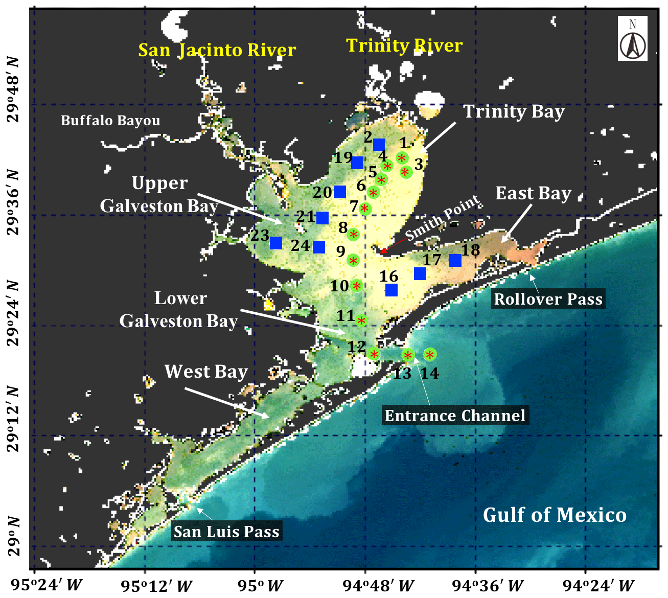
Figure 1Sentinel-3A OLCI RGB image (29 October 2017) with locations of sampling sites in Galveston Bay acquired on 29 September (red asterisk), 29 October (green circles) and 30 October 2017 (blue solid squares), respectively.
2.1 Study area
Galveston Bay (GB), a shallow water estuary (∼2.1 m average depth), encompasses two major sub-estuaries: San Jacinto Estuary (also divided as Upper GB and Lower GB) and Trinity Estuary (Trinity Bay) (Fig. 1). It is located adjacent to the heavily urbanized and industrialized metropolitan areas of Houston, Texas (Dorado et al., 2015). The deep (∼14 m) narrow Houston Ship Channel connects the bay to the northern Gulf of Mexico (nGoM) through a narrow entrance, the Bolivar Roads Pass. Tidal exchange between GB and the nGoM occurs through the entrance channel with diurnal tides ranging from ∼0.15 to ∼0.5 m. The major freshwater sources to GB are the Trinity River (55 %), the San Jacinto River (16 %) and Buffalo Bayou (12 %) (Guthrie et al., 2012). The San Jacinto River was frequently observed to transport greater amounts of dissolved nutrients into GB than the Trinity River (Quigg, 2011); however, the negative relationship between nitrate concentrations and salinity observed in the mid-bay area (adjacent to Smith Point) (Santschi, 1995) indicated Trinity River to be a major source of nitrate in GB. The catastrophic flooding of Houston and surrounding areas associated with Hurricane Harvey resulted in strong freshwater inflows into GB from the San Jacinto River (>3300 m3 s−1; USGS 08067650) on 29 August 2017 and the Trinity River (>2500 m3 s−1; USGS 08066500 site at Romayor, Texas) on 30 August 2017, respectively. Although the discharge from the two rivers in the upstream returned to normal conditions (∼50–120 m3 s−1) in about 2 weeks after the Hurricane passage, salinity remained low for over a month following the hurricane passage (D'Sa et al., 2018).
2.2 Sampling and data collection
Surface water samples were collected at a total of 34 stations during two surveys on 29 September and 29–30 October 2017 (Fig. 1). Samples at stations 1 to 14 (red asterisk on top of green circle; Fig. 1) along the Trinity River transect were collected repeatedly on 29 September and 29 October 2017, respectively. An additional nine sampling sites (blue squares; Fig. 1) around the upper Galveston Bay and in the East Bay were sampled on 30 October 2017. The surface water samples were stored in coolers and filtered on the same day. The filter pads were immediately frozen and stored in liquid nitrogen for laboratory absorption spectroscopic and HPLC measurements of the samples. An optical package equipped with a conductivity–temperature–depth recorder (SBE; Sea-Bird Scientific) and a fluorescence induction and relaxation system (FIRe; Satlantic Inc.) were used to obtain profiles of salinity, temperature, pressure and phytoplankton physiological parameters (Fv∕Fm and σPSII). Measurements of backscattering were also made at each station using the WETLabs VSF-3 (470, 530, 670 nm) backscattering sensor (D'Sa et al., 2006). Included in the optical package was also a hyperspectral downwelling spectral irradiance meter (HyperOCR; Satlantic Inc.). The irradiance data from the HyperOCR were processed using ProSoft 7.7.14 and the photosynthetically active radiation (PAR) were estimated from the irradiance measurements. The above-water reflectance measurements were collected using a GER 1500 512iHR spectroradiometer in the 350–1050 nm spectral range. At each station, sky radiance, plate radiance and water radiance were recorded (each repeated three times) and processed to obtain the above-water remote-sensing reflectance (Joshi et al., 2017). A total of 43 Sentinel-3A OLCI full resolution mode, cloud free level-1 images were obtained over GB between 1 August 2016 and 1 December 2017 from the European Organisation for the Exploitation of Meteorological Satellites (EUMETSAT) website and pre-processed using Sentinel-3 Toolbox Kit Module (S3TBX) version 5.0.1 in Sentinel Application Platform (SNAP). These Sentinel-3A OLCI data were further atmospherically corrected to obtain remote-sensing reflectance (, sr−1) using Case-2 Regional/Coast Color (C2RCC) module version 0.15 (Doerffer and Schiller, 2007). River discharge information during August 2016–December 2017 was downloaded from the USGS Water Data (USGS) for the Trinity River at Romayor, Texas (USGS 08066500), and the west flank of the San Jacinto River (USGS 08067650). Individual pictures of microplankton (10 to 150 µm) recorded by an Imaging FlowCytobot (IFCB) located at the entrance to Galveston Bay were downloaded (http://dq-cytobot-pc.tamug.edu/tamugifcb, last access: 8 November 2018) for pigment validation.
2.3 Absorption spectroscopy
Surface water samples were filtered through 0.2 µm nuclepore membrane filters, and the colored dissolved organic matter (CDOM) absorbance (ACDOM) was obtained using a 1 cm path length quartz cuvette on a PerkinElmer Lambda-850 UV–VIS spectrophotometer equipped with an integrating sphere. The quantitative filter technique (QFT) with 0.7 µm GF/F filters was used to measure absorbance of particles (Atotal) and non-algal particles (ANAP) inside an integrating sphere at 1 nm intervals from 300 to 800 nm. The absorption coefficients of CDOM (aCDOM), NAP (aNAP), particles (atotal) and phytoplankton (aPHY) were calculated using the following equations:
where L is the path length in meters. The aCDOM were corrected for scattering, temperature and baseline drift by subtracting an average value of absorption between 700 and 750 nm for each spectrum (Joshi and D'Sa, 2015).
where Vfiltered is the filtered volume of sample, Sfilter is the area of filter pads and the path length correction for filter pad was applied according to Stramski et al. (2015).
2.4 Pigment absorption spectra
The water samples were filtered with 0.7 µm GF/F filter. The filter pads were stored in liquid nitrogen until transferred into 30 mL vials containing 10 mL cold 96 % ethanol (Ritchie, 2006). The vials were spun evenly to ensure full exposure of the filter pad to the ethanol and then kept in the refrigerator (in the dark) overnight. The pigment solutions at room temperature were poured off from vials into 1 cm cuvettes and measured on a PerkinElmer Lambda-850 UV–VIS spectrophotometer to obtain pigment absorbance spectra (Apig) while 90 % ethanol was used as a blank (Thrane et al., 2015). The total absorption coefficients of pigments apig(λ) were calculated as follows:
where L is the path length in meters, Vethanol is the volume of ethanol and Vfiltered is the filtered volume of the water samples.
2.5 HPLC measurements
Water samples were filtered through 0.7 µm GF/F filters and immediately frozen in liquid nitrogen for HPLC analysis using the methods reported by Barlow et al. (1997). The detected pigments along with their abbreviations are listed in Table 1. Diagnostic biomarker pigments are marked in bold letters (Table 1).
Table 1Pigment information acquired from HPLC samples in Galveston Bay. Diagnostic biomarker pigments are marked in bold.
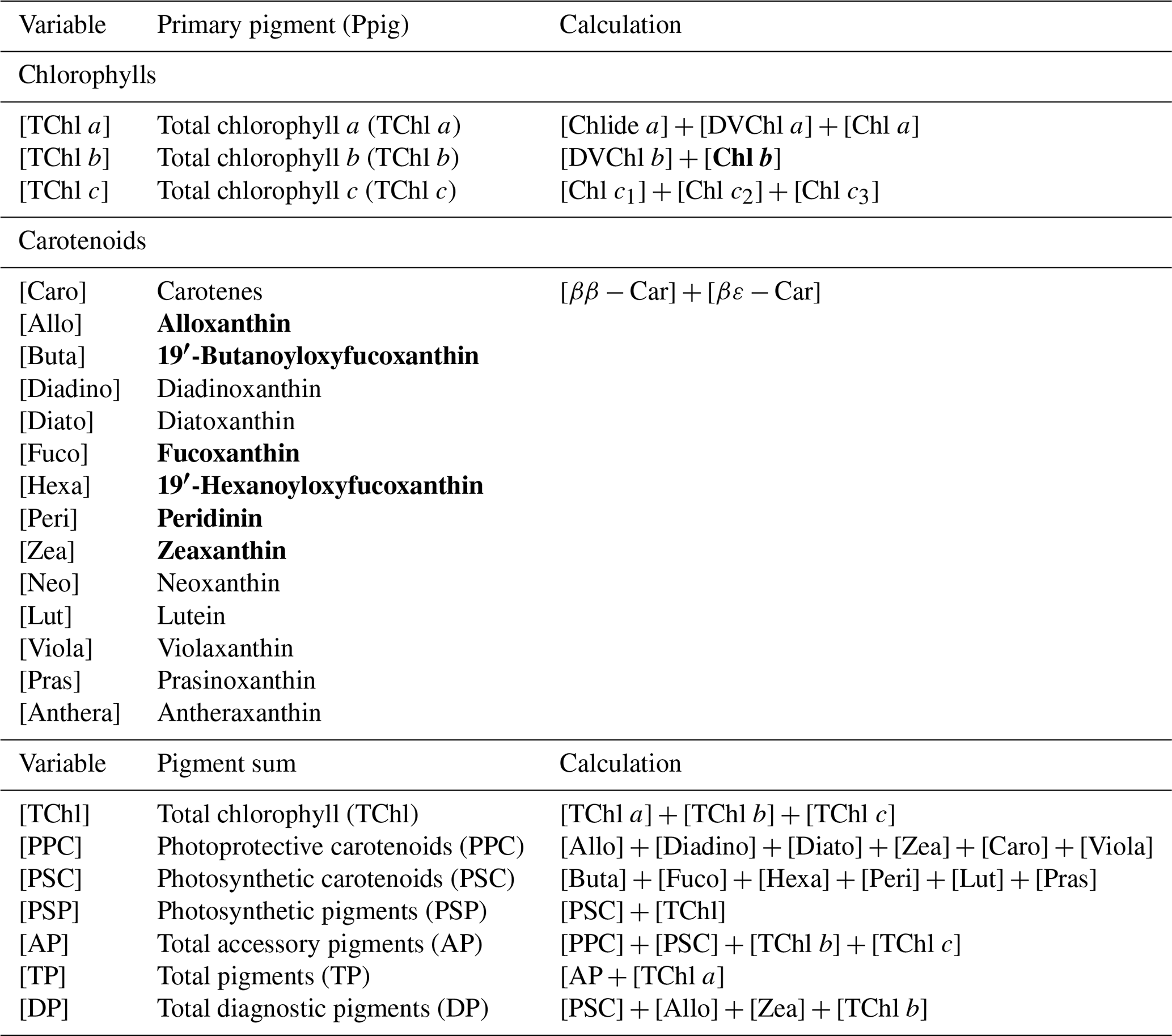
Note: (1) [Chl b], [Allo], [Fuco], [Peri], [Zea], [Buta] and [Hexa] are considered as diagnostic pigments for PFTs (Moisan et al., 2017).
2.6 FIRe measurements
An in situ FIRe system (Satlantic Inc.) was used to characterize phytoplankton photosynthetic physiology during the two surveys in GB. The FIRe system is based on illuminating a sample with an intense flash of light to instantaneously saturate the reaction centers of photosystem II (PSII); under these light conditions, reaction centers do not accept electrons and most of the absorbed light energy is dissipated as fluorescence. The fundamental parameter measured by the FIRe system is fluorescence yield F(t), which is the emitted fluorescence divided by the irradiance intensity (no unit). In contrast to strong flashes, dark adaption enables all reaction centers of PSII to be open with least fluorescence emitted, thus resulting in minimal fluorescence yield (Fo). Maximum fluorescence yield (Fm) can be obtained after sufficient irradiation when all reaction centers are closed. Maximum photochemical efficiency, which quantifies the potential of converting light to chemical energy for the PSII reaction centers (Moore et al., 2006), was calculated as (. The functional absorption cross section σPSII (Å2quantum−1) measures the capability of reaction centers to absorb light from the ambient environment. The FIRe system was deployed at a slow descent rate, with 12 and 20 vertical profiles obtained during the first and second surveys, respectively. All measurements were programmed using standard protocols of single saturating turnover (ST) flash saturation of PSII (Kolber et al., 1998). Flashes were generated from highly uniform blue LEDs at 455 nm with approximately 30 nm half-bandwidth. Chl a fluorescence was stimulated using a saturating sequence of 80 1.1 µs flashes applied at 1 µs intervals, eight sequences were averaged per acquisition, and the fluorescence signal was detected at 668 nm. All data were processed using standard FIReCom software (Satlantic Inc.). In addition, samples of 0.2 µm filtered sea water at each station were used as “blank” to remove the background fluorescence signals (Cullen and Davis, 2003); in this step, the fluorescence from the filtered samples (without phytoplankton) was subtracted from in situ fluorescence signals to get more accurate values of Fv∕Fm.
2.7 Retrieving phytoplankton groups from above-water Rrs
A fundamental relationship that links subsurface remote-sensing reflectance (rrs) and the IOPs was expressed using a quadratic function developed by Gordon et al. (1988):
where the parameters g1 (∼0.0788) and g2 (∼0.2379) are values for turbid estuarine waters (Joshi and D'Sa, 2018); rrs is the subsurface remote-sensing reflectance that was obtained from above-water remote-sensing reflectance (Rrs) using the following equation (Lee et al., 2002)
The total backscattering coefficient bb is comprised of water (bbw) and particulates including both organic and inorganic particles (bbp), while the total absorption coefficients (atotal) can be further separated into four sub-constituents (Roesler and Perry, 1995) as indicated by
where aw, aphy, aCDOM, and aNAP represent the absorption coefficients of pure water, phytoplankton, colored dissolved organic matter and non-algal particles, respectively.
The IOP inversion algorithm for retrieving IOPs from Rrs require known spectral shape (eigenvector) of each component in Eq. (8) to estimate the magnitude (eigenvalue) of each component (Table 2). The spectral shape can be adjusted by changing the values of slope based on characteristics of the study area. It is worth noting that a single averaged phytoplankton eigenvector does not provide species information, whereas a set of several species-specific phytoplankton eigenvectors allow estimates of species composition. The IOP inversion algorithm applied in this study makes use of mass-specific phytoplankton absorption spectra of 10 groups, namely dinoflagellates, diatoms, chlorophytes, cryptophytes, haptophytes, prochlorophytes, raphidophytes, rhodophyta, red cyanobacteria and blue cyanobacteria; these were obtained from Dierssen et al. (2006) and Dutkiewicz et al. (2015) as eigenvectors rather than using one averaged aphy(λ) spectrum. Subsequently, the inversion algorithm iterates repeatedly to minimize the difference between modeled Rrs and in situ measured Rrs (Rrs_insitu) until a best fit is achieved while allowing for alterations of all parameters listed in Table 2 (Chase et al., 2017). The absolute percent errors between modeled and measured values of Rrs, aphy, aCDOM, aNAP and bbp were calculated as
2.8 Retrieving pigments from Sentinel-3A OLCI Rrs
2.8.1 Reconstruction of pigment absorption spectrum by multiple linear regression
Total pigment absorption spectra apig(λ) obtained during both surveys (Eq. 5) were modeled as a third-order function of HPLC measured-Chl a (Chl a_HPLC) concentration at each station as (Moisan et al., 2017)
where vector coefficient , are wavelength-dependent coefficients that range from 400 to 700 nm at 1 nm intervals; these were further applied to Sentinel-3A OLCI Chl a to calculate apig_OLCI at each pixel as
where Chl a_OLCI is Sentinel-3A OLCI derived Chl a concentration (259×224 pixels). The obtained image represents the value of apig_OLCI at a certain wavelength and 301 images of apig_OLCI can be obtained in the 400–700 nm wavelength range at 1 nm intervals.
2.8.2 Satellite retrieval of pigments using non-negative least squares (NNLS) inversion model
The apig_OLCI is a mixture of n pigments with known absorption spectra ai(λ), at wavelength λ (nm); thus, apig_OLCI(λ) can be considered as a weighted sum of the individual component spectra (Thrane et al., 2015) at each image point as
where represents the mass-specific spectra of 16 pigments (Chl a, Chl b, Chl c1, Chl c2, pheophytin a, pheophytin b, peridinin, fucoxanthin, neoxanthin, lutein, violaxanthin, alloxanthin, diadinoxanthin, diatoxanthin, zeaxanthin and β-carotenoid) which are the in vitro pigment absorption spectra over pigment concentrations and can be extracted from supplementary R scripts of Thrane et al. (2015). The vector coefficient corresponds to the concentrations (µg L−1) of these distinct pigments; note that X cannot be negative, therefore non-negative least squares (NNLS) was used to guarantee positive solutions of X (Moisan et al., 2013; Thrane et al., 2015). Equation (12) can be further expressed as
2.9 Processing approach
Sentinel-3A OLCI pigment concentration maps were generated using the processing pathway 1 (Fig. 2) that includes the following: (1) developing empirical relationships between HPLC-measured Chl a and Rrs_insitu band ratio for Sentinel-3A OLCI band 9 (673 nm) and band 11 (709 nm) to generate Sentinel-3A OLCI Chl a maps and (2) converting Chl a concentration to apig_OLCI(λ) maps and subsequently decomposing apig_OLCI(λ) into individual pigment spectra to generate phytoplankton pigment maps for GB. In processing pathway 2, phytoplankton taxonomic composition at each sampling station was obtained from a 10-species IOP inversion model, which uses Rrs_insitu as input and estimates Chl a concentration of each phytoplankton group (Fig. 2). Finally, CDOM-corrected FIRe measurements of Fv∕Fm and σPSII were combined with phytoplankton taxonomy to assess photosynthetic physiology of different phytoplankton groups.
Table 2Parameters and eigenvectors used in the semi-analytical inversion algorithm.
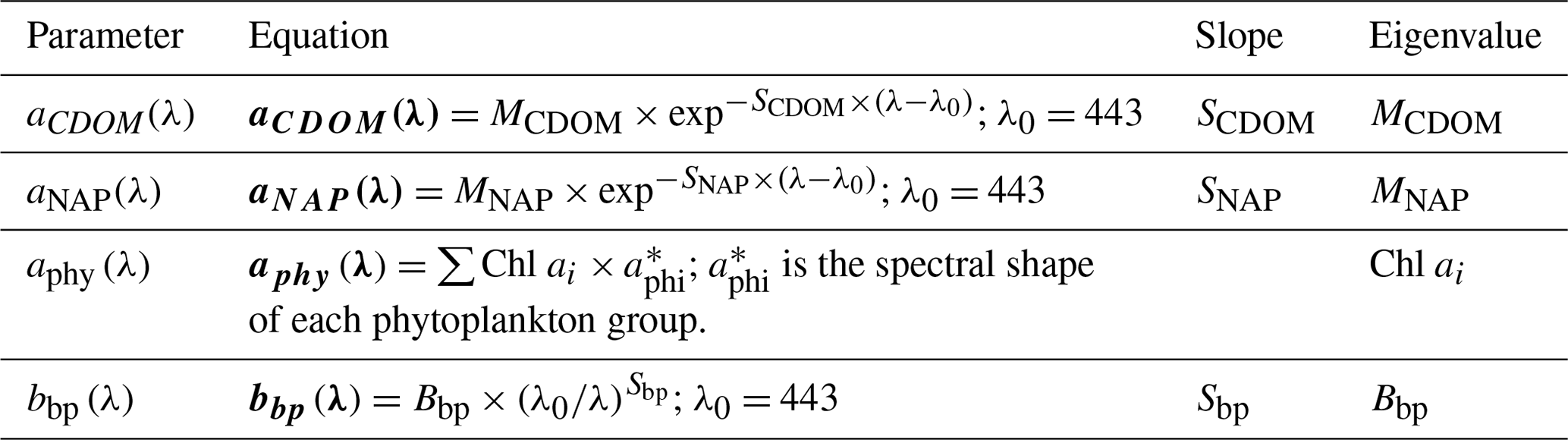
Note: for 10 different groups of phytoplankton used in this study were extracted from Dierssen et al. (2006) and Dutkiewicz et al. (2015).
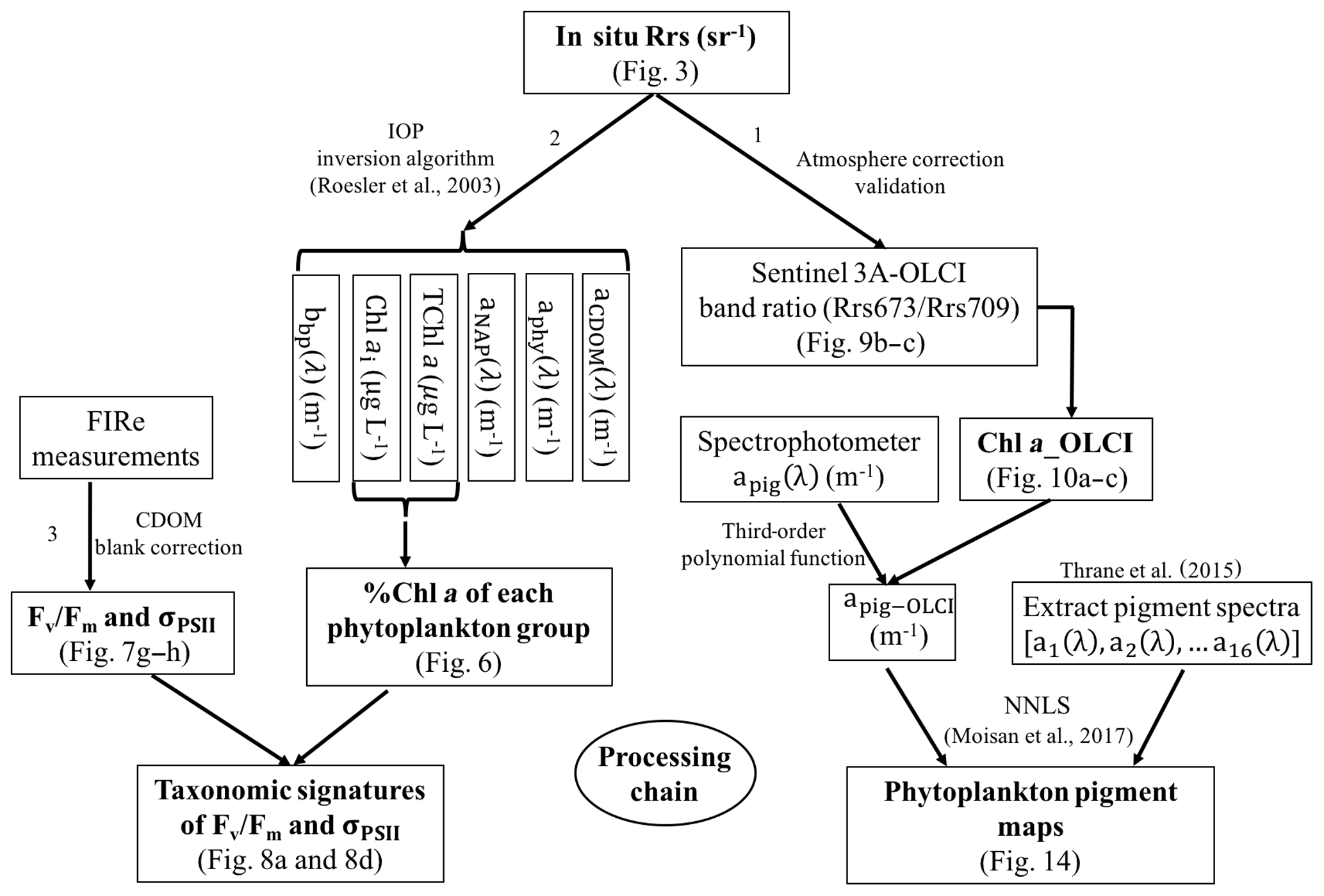
Figure 2Flowchart showing the three processing steps as follows: (1) retrieving pigments spatial distribution maps from OLCI, (2) distinguishing phytoplankton groups, and (3) assessing phytoplankton physiological parameters and their linkages to taxonomic groups.
3.1 Phytoplankton taxonomy and physiological state from field observations
3.1.1 Measurements of above-water remote-sensing reflectance
Above-water remote-sensing reflectances (Rrs_insitu) from the two surveys (Fig. 3) reflect the influence of the absorbing and scattering features of water constituents. Low reflectance (∼675 nm) caused by Chl a red light absorption and maximum reflectance at green wavelength (∼550 nm) were observed. Obvious dips at ∼625 nm versus reflectance peaks ∼650 nm were observed in spectra during both surveys, which could be attributed to cyanobacteria modulation of the spectra (Hu et al., 2010). The reflectance peak around 690–700 nm was obvious at most sampling sites except at stations 13 and 14 adjacent to the nGOM and were likely due to the effect of Chl a fluorescence (Gitelson, 1992; Gilerson et al., 2010). The peak positions at stations with lower Chl a concentration (∼5 µg L−1) were observed at 690–693 nm; however, the peaks shifted to longer wavelengths of 705 and 710 nm for stations 23 and 19 with extremely high Chl a concentrations of ∼31 and 50 µg L−1, respectively (Fig. 3).
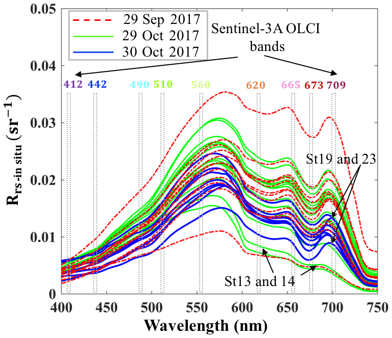
Figure 3Rrs_insitu spectra at stations in GB on 29 September and 29–30 October 2017; vertical bars represent Sentinel-3A OLCI spectral bands.
3.1.2 Performance of the IOP inversion algorithm
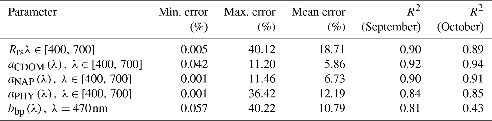
The IOP inversion algorithm was applied to Rrs_insitu data (Fig. 3) obtained during the two surveys in GB. The mean errors for modeled aCDOM, aNAP, aphy and bbp_470 at all wavelengths for the 34 stations were 5.86 %, 6.83 %, 12.19 % and 10.79 %, respectively (Table 3). A total of eight phytoplankton groups (dinoflagellate, diatom, chlorophyte, cryptophyte, haptophyte, prochlorophyte, raphidophyte and blue cyanobacteria) were spectrally detected from IOP inversion algorithm. The sum of eight eigenvalues of Chli (Table 2) represents the modeled total Chl a (TChl a_mod) of the whole phytoplankton community. The TChl a_mod is better correlated with HPLC-measured total Chl a (TChl a_HPLC) for survey 2 (green circle; Fig. 4a) with R2∼0.92, compared to survey 1 (red color; Fig. 4a). In addition, the TChl a_mod appears to be slightly higher than TChl a_HPLC for survey 2. The modeled aCDOM (aCDOM_mod) are in close agreement with the spectrophotometrically measured aCDOM at 412 nm (Fig. 4b), with the aCDOM obtained on 29 September 2017 much higher than that obtained on 29–30 October 2017. The modeled bbp (bbp_mod) are well correlated with in situ bbp (bbp_insitu) at 470 nm (Fig. 4c) with higher R2 (0.81) observed on 29 September 2017. In addition, both modeled and field-measured bbp showed stronger backscattering at most stations on 29 September 2017 than those on 29–30 October 2017.

Figure 4(a) Validation of TChl a_mod via HPLC-measured TChl a; individual %Chl a of each detected taxa versus corresponding %DP shown with (d) cryptophyte, (e) chlorophyte, (f) cyanobacteria, (g) diatom, (h) dinoflagellate and (l) haptophyte; red and green dots indicate the samples on 29 September and 29–30 October 2017, respectively. Comparison between in situ measurements and modeled results with (b) aCDOM (412) and (c) bbp (470).
Table 3Error statistics over all wavelengths and sampling stations (; 12 and 22 stations on 29 September and 29–30 October 2017) from a semi-analytical IOP inversion algorithm.
The Chl a percentage (%Chl a), which is Chli ∕ TChl a, was also compared with diagnostic pigment percentage (%DP), which is the specific DP for each phytoplankton group over the sum of DP (∑DP). The DP for diatoms (fucoxanthin), dinoflagellates (peridinin), cryptophytes (alloxanthin), chlorophytes (Chl b), haptophytes (19′-hexanoyloxyfucoxanthin) and cyanobacteria (zeaxanthin) referred in Moisan et al. (2017) were used in this study. The R2 between %Chl a and %DP for different phytoplankton groups ranges from 0.15 to 0.81 (Fig. 4). The %Chl a of cryptophytes is between 5 % and 42 % and is well correlated with alloxanthin ∕ ∑DP (R2∼0.62–0.72; Fig. 4d) for both surveys. In addition, the cryptophyte %Chl a at station 19 and 23 on 30 October 2017 was highest (∼40 %) in coincidence with the highest value of alloxanthin ∕ ∑DP (Fig. 4d). Furthermore, the relationship between chlorophyte %Chl a and Chl b ∕ ∑DP (R2∼0.55; Fig. 4e) shows that chlorophytes during survey 1 contributed a higher fraction to the whole phytoplankton community compared to survey 2. The %Chl a of cyanobacteria highly correlated with zeaxanthin ∕ ∑DP with R2 larger than 0.7 (Fig. 4f) for both surveys. Low %Chl a of dinoflagellates in coincidence with low peridinin ∕ ∑DP (R2∼0.78) were observed at stations along the transect; however, an increased contribution of dinoflagellates appeared adjacent to the entrance during both surveys (Fig. 4g).
3.1.3 Variations in phytoplankton community structure
Reconstruction of the phytoplankton absorption coefficients spectra revealed variations in phytoplankton community structure (Fig. 5) even several weeks after Hurricane Harvey. The modeled aphy spectra (aphy_mod) at stations 6, 13, 17 and 19 (Fig. 5a–f) yielded spatiotemporal differences of phytoplankton taxonomic composition in GB. The strong absorption peak around 625 nm induced by cyanobacteria was observed at most of the stations for both modeled results and in situ measurements (Fig. 5a, c and e) except at stations adjacent to the entrance (Fig. 5b and d). The aphy_mod at station 6 was primarily dominated by group of cyanobacteria (blue line) and chlorophytes (green line) on 29 September 2017 (Fig. 5a); in contrast, the spectrum of chlorophytes contributed very little at station 6 on 29 October 2017 (green line; Fig. 5c). Furthermore, the shape of spectra for samples obtained at station 13 shows strong dinoflagellate modulation versus extremely low cyanobacteria contribution during survey 1 (red line; Fig. 5b). However, small-size groups like the haptophytes and prochlorophytes displayed increasing proportions at station 13 on 29 October 2017 (Fig. 5d). Station 17 in the East Bay was dominated by cyanobacteria (blue line; Fig. 5e) and cryptophyte (pink line; Fig. 5e) absorption spectra, whereas, on 30 October 2017, the main spectral features at station 19 in the upper GB was from cryptophytes (pink line) and chlorophytes (green line; Fig. 5f).
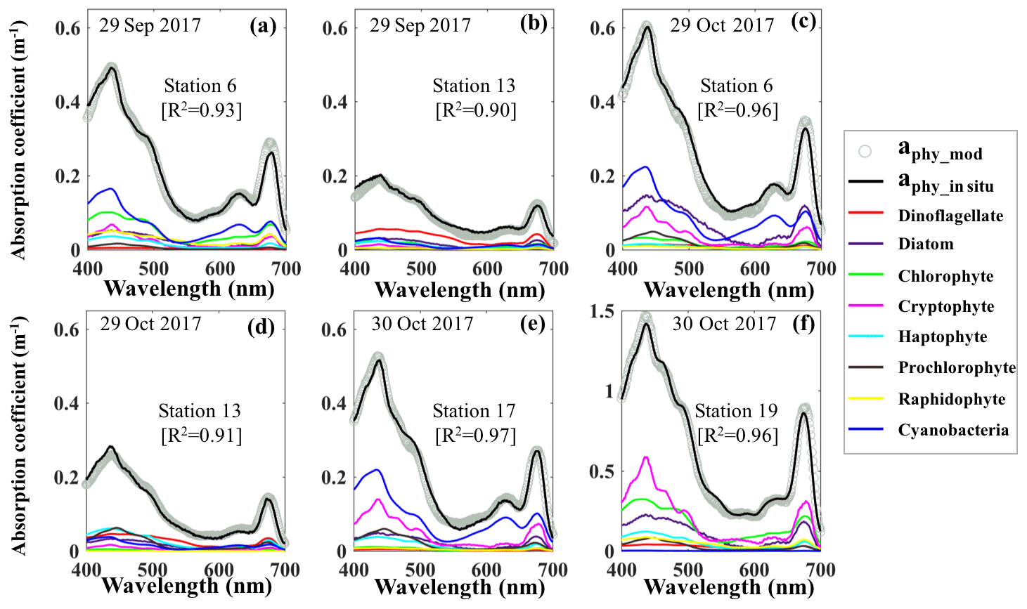
Figure 5Reconstruction of phytoplankton absorption coefficients spectra at stations 6 (a) and 13 (b) on 29 September 2017, at stations 6 (c) and 13 (d) on 29 October 2017 and at stations 17 (e) and 19 (f) on 30 October 2017 based on the mass-specific absorption spectra of different phytoplankton groups including diatoms, chlorophytes, dinoflagellates, cryptophytes, cyanobacteria (blue), haptophytes, prochlorophytes and raphidophytes presented using different colors.
The corresponding taxa-specific %Chl a derived from IOPs inversion algorithm for the two surveys on 29 September and 29–30 October 2017 are shown in Fig. 6a and b, respectively. Cyanobacteria (blue bars) and chlorophytes (green bars) constituted over 55 % of the phytoplankton communities during survey 1 (29 September 2017; Fig. 6a). In addition, chlorophytes, known to proliferate in freshwater environments, were present in a higher fraction than that observed in survey 2 (Fig. 6). Further, chlorophytes together with diatoms (Fig. 6a) accounted for ∼60 % of TChl a_mod at many stations with a well-mixed water column (e.g., stations 7, 8 and 9 as inferred from salinity profiles; not shown) on 29 September 2017. Cryptophytes, haptophytes and raphidophytes became minor components of the community and accounted in total to ∼25 % of TChl a_mod (Fig. 6a). Furthermore, contribution by the dinoflagellate group to TChl a_mod was low inside the bay, but showed increasing %Chl a (∼30 %) in higher-salinity waters adjacent to the nGOM (red color; Fig. 6a). Cyanobacteria (blue color; Fig. 7) exhibited a slightly elevated percentage during survey 2 (∼60 d after the hurricane passage, 29–30 October 2017) and were quite abundant in East Bay (stations 16, 17 and 18) where the water was calm and stratified (as indicated by the salinity profiles – not shown). In addition, cyanobacteria were not prevailing adjacent to the nGOM (stations 12, 13 and 14) and close to San Jacinto (stations 19, 20, 21, 23 and 24), where cryptophytes and chlorophytes showed dominance (Fig. 6b). The %Chl a of chlorophytes obtained at stations along the Trinity River transect decreased by ∼10 % on 29–30 October 2017 compared to 29 September 2017. Small-size groups like haptophytes and prochlorophytes increased on 29–30 October 2017 and were more abundant adjacent to the nGOM, accounting for more than 25 % of the TChl a_mod.
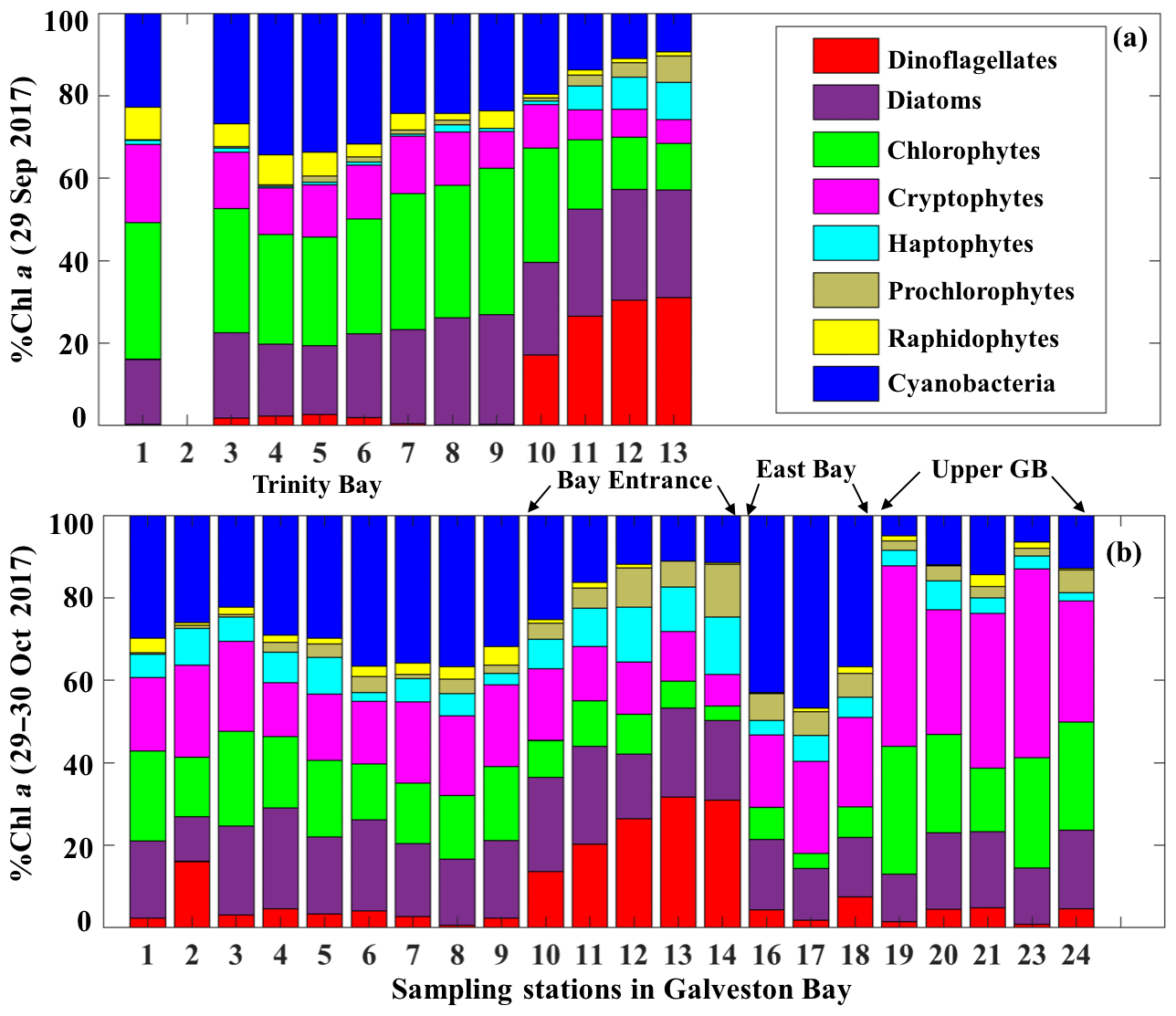
Figure 6Phytoplankton taxonomic compositions detected from IOP inversion algorithm on (a) 29 September and (b) 29–30 October 2017 in Galveston Bay; phytoplankton groups are represented in different colors as shown in the legend.
3.1.4 Environmental conditions and physiological state of phytoplankton community
The surface salinity presented a pronounced seaward increasing gradient along the transect (stations 3–14) during both surveys (Fig. 7a) with primarily lower salinity throughout the bay during survey 1 in comparison to survey 2, which indicated the freshening impact was still ongoing even 4 weeks after Hurricane Harvey. The salinity was ∼15 at station 16 and decreasing when going further into East Bay (∼10 at stations 17 and 18; Fig. 7a). In upper GB, salinity at stations 19–24 did not vary significantly (∼15), increasing along with the distance away from the San Jacinto River mouth with highest value (∼17.5) at station 24. During both surveys, lowest Chl a (Fig. 7b) were observed adjacent to the nGOM, and the highest Chl a were closest to the river mouth. The photosynthetically active radiation (PAR), which were calculated from down-welling irradiance (not shown here), decreased significantly with depth, but surface PAR (Fig. 7c) were similar in magnitude at all stations. Pigment ratios including TChl a ∕ TP (0.58–0.68), PSC ∕ Chl a (0.07–0.26) and AP ∕ TP (0.34–0.42) were obtained from HPLC measurements and shown in Fig. 7d, e and f, respectively.
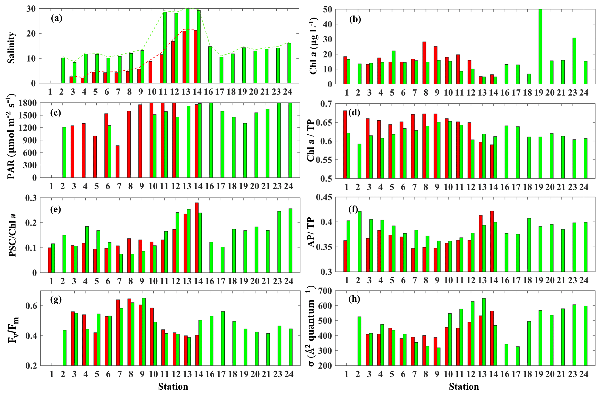
Figure 7Environmental conditions (salinity, light field), pigment composition and physiological state in GB surface waters (red bars indicating samples from 29 September 2017 and blue bars representing samples from 29 and 30 October 2017). (a) Salinity, (b) Chl a concentration, (c) PAR, (d) Chl a ∕ TP, (e) PSC ∕ Chl a, (f) AP ∕ TP, (g) Fv∕Fm and (h) σPSII.
The CDOM-calibrated and 0–0.5 m depth-averaged photosynthetic parameters Fv∕Fm varied from 0.41 to 0.64 (Fig. 7g) while σPSII was in the range of 329–668 Å2quantum−1(Fig. 7h). The highest σPSII and lowest Fv∕Fm appeared adjacent to the nGOM (stations 12–14). Conversely, values of Fv∕Fm at stations 7–9 with a well-mixed water column were high with low values of σPSII. Both Fv∕Fm and σPSII did not directly correlate with Chl a (e.g., high Chl a∼51 µg L−1 at station 19 corresponded to a relatively low level of versus high σPSII∼550 Å2quantum−1). However, the stations with high Fv∕Fm coincided with the high fraction of Chl a (Chl a ∕ TP) and the low fraction of AP (AP ∕ TP) (Fig. 7d and f). In contrast, σPSII showed an overall positive relationship with AP ∕ TP but altered negatively with Chl a ∕ TP during both surveys. The lowest (highest) value of σPSII (Fv∕Fm) were observed at station 9, corresponding to the highest Chl a ∕ TP value (∼0.64) on 29 October 2017. The highest AP ∕ TP and PSC ∕ Chl a were obtained from stations adjacent to the nGOM.
3.1.5 Fv∕Fm and σPSII taxonomic signatures
Distinct pigments housed within phytoplankton light-harvesting antennae can strongly influence PSII light-harvesting capability and the photosynthetic quantum efficiency of phytoplankton (Lutz et al., 2001). In this study, we observed an inverse relationship (R2∼0.63–0.81; Fig. 8a and d) between the Fv∕Fm and σPSII that appeared related to taxonomic signals during surveys 1 and 2 in GB. Stations 1–9 along the transect were considered as a well-mixed group with no dominance by any particular group (black circles; Fig. 8a–c); stations 10–14 close to the entrance were, however, strongly dominated by dinoflagellates and haptophytes (red symbol; Fig. 8a–c) during survey 1. This well-mixed group displayed low values of σPSII (∼390–439 Å2quantum−1) and high levels of Fv∕Fm (∼0.42–0.65), with Fv∕Fm approaching 0.65 at station 9 on 29 September 2017 (Fig. 8a). However, enhanced contributions of dinoflagellates and haptophytes around the entrance corresponded to a decline of Fv∕Fm (0.3–0.4) against an increase of σPSII (500–600 Å2quantum−1) during survey 1. Furthermore, samples obtained from survey 2 at stations 1–9, stations 10–14, stations 16–18 and stations 19–24 were considered as well mixed (black), dinoflagellate–haptophyte-dominated (red), cyanobacteria-dominated (blue) and cryptophyte–chlorophyte-dominated (green), respectively. Stations 16–17 dominated by cyanobacteria (blue triangles; Fig. 8d) showed high level of Fv∕Fm (0.5–0.6) and relatively low values of σPSII (300–400 Å2quantum−1). The Fv∕Fm and σPSII of cryptophyte–chlorophyte-dominated stations showed a moderate level of Fv∕Fm (0.4–0.5) and σPSII (580–680 Å2quantum−1). More importantly, tight positive relationships existed between measurements of Fv∕Fm and Chl a ∕ TP (R2∼0.31–0.63; Fig. 8b and e). On the other hand, σPSII values were positively correlated with the PSC ∕ Chl a with R2∼0.6 (Fig. 8c and f). The PSC ∕ Chl a of cyanobacteria-dominated group (blue symbols) and the well-mixed group (brown symbols) were relatively low. The highest PSC ∕ Chl a and lowest Chl a ∕ TP values were observed for the dinoflagellate–haptophyte-dominated group, corresponding to the lowest σPSII and the highest Fv∕Fm. In addition, the cryptophyte–chlorophyte-dominated group had high levels of PSC/TChl a (∼0.18–0.26) and a slightly higher Chl a ∕ TP level compared to the dinoflagellate–haptophyte-dominated group. Overall, well-mixed groups with high proportion of large-size phytoplankton (e.g., diatoms and chlorophytes) showed higher Chl a ∕ TP levels along with larger Fv∕Fm and smaller σPSII values than those stations with a high fraction of dinoflagellates and picophytoplankton (e.g., haptophytes and prochlorophytes)(Fig. 8c and f).
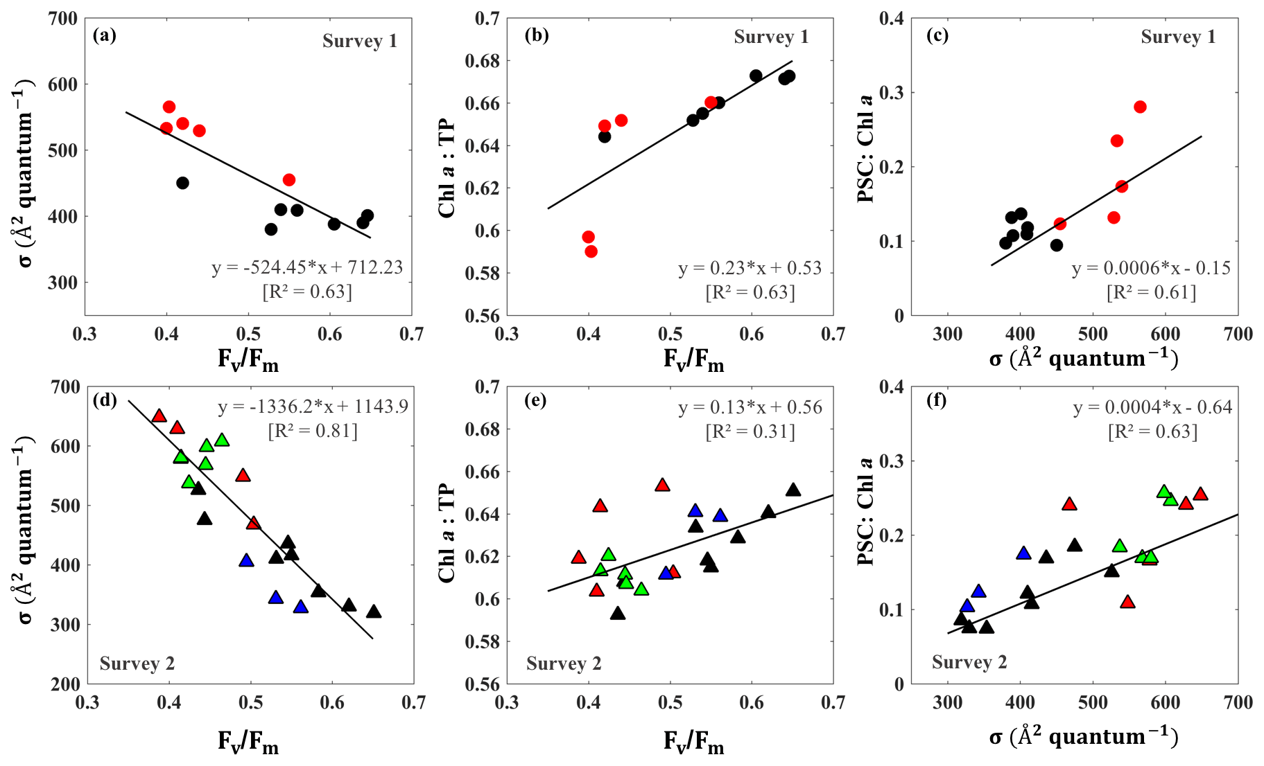
Figure 8(a, d) σPSII vs. Fv∕Fm; (b, e) Fv∕Fm versus Chl a ∕ TP; and (c, f) σPSII versus PSC ∕ Chl a on 29 September and 29–30 October 2017, respectively. The data points identified by dominant taxa with black, red, green and blue symbols denoting well-mixed, dinoflagellate–haptophyte-dominated, cryptophyte–chlorophyte-dominated and cyanobacteria-dominated groups, respectively.
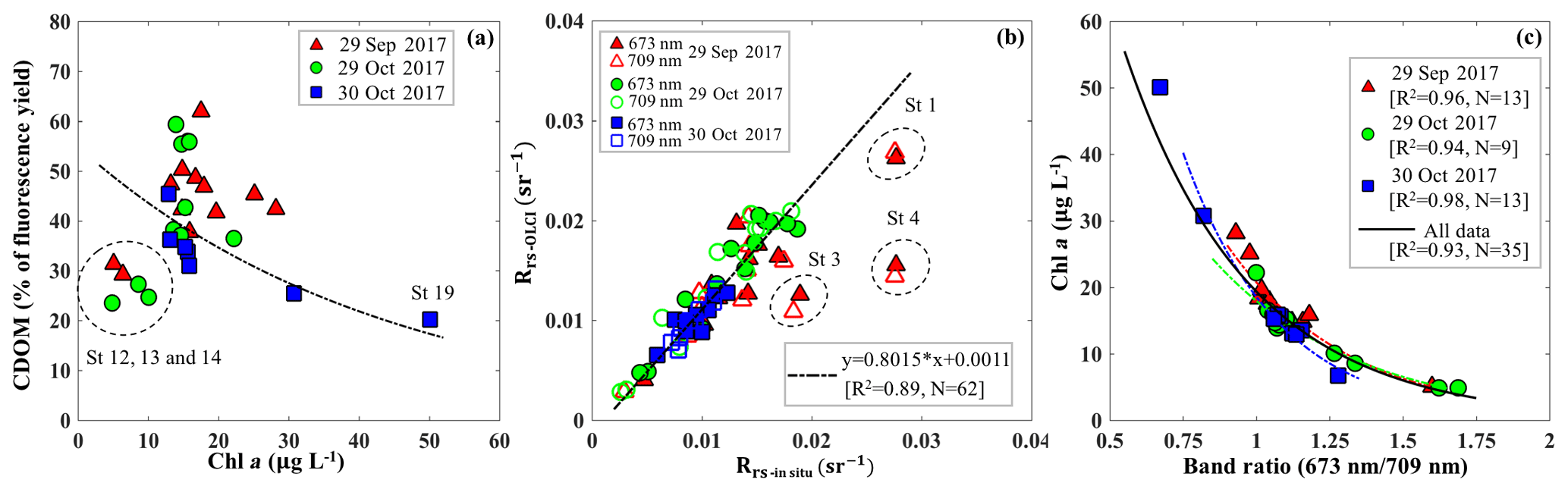
Figure 9(a) Relationship between the percentage of the fluorescence yield of CDOM measured by FIRe against HPLC-measured Chl a concentration. The dashed circle corresponds to data acquired in the area adjacent to the GOM. (b) Comparisons between Rrs_insitu and Rrs_OLCI at band 9 (673 nm) and band 11 (709 nm). The dashed circles correspond to stations 1, 3 and 4 located close to the river mouth and are considered as outliers. (c) Exponential relationships between HPLC-measured Chl a concentrations and Rrs_insitu band ratio (673 nm ∕ 709 nm) in GB on September 29 (R2=0.89), 29 October (R2=0.93) and 30 October (R2=0.97). Red, green and blue lines and symbols indicate data sets obtained on 29 September, 29 October and 30 October 2017, respectively.
3.2 Satellite observations of phytoplankton pigments
3.2.1 An OLCI Chl a algorithm and its validation
Blue to green band ratio algorithms have been widely used to study Chl a in the open ocean and shelf waters (D'Sa et al., 2006; Blondeau-Patissier et al., 2014); however, these bands generally fail in estuarine waters due to strong blue absorption by the high levels of CDOM and suspended particulate matter, especially after flooding events associated with hurricanes (D'Sa et al., 2011, 2018; Joshi and D'Sa, 2018). The percentage contribution by CDOM fluorescence (blank) to maximum fluorescence yield (Fm) obtained from in situ FIRe (Fig. 9a) demonstrated that Chl a fluorescence was strongly influenced by high amounts of CDOM fluorescence in GB, especially during the first survey (29 September 2017) when the bay was under strong floodwater influence (red triangles; Fig. 9a). The CDOM fluorescence signal constituted ∼25 % in the region adjacent to the nGOM (stations 12–14), between 25 % and 50 % in the upper GB and up to ∼65 % in Trinity Bay, which implies that blue and even green bands are highly contaminated by CDOM and might not be the most suitable bands for estimating Chl a in GB. However, an increase in peak height near 700 nm and its shift towards a longer wavelength (Fig. 3) can be used as a proxy to estimate Chl a concentration (Gitelson, 1992).
The C2RCC atmospheric-corrected Rrs_OLCI at each of the sampling sites were further compared with Rrs_insitu (Fig. 3) at phytoplankton red absorption (∼673 nm) and Chl a fluorescence (∼700 nm) bands (Fig. 9b). The C2RCC performed overall better for the second survey on 29–30 October 2017 (green and blue symbols; Fig. 9b) than the first survey on 29 September 2017 (red triangles; Fig. 9b) when stations 1, 3 and 4 (circled triangles; Fig. 3c) adjacent to the Trinity River mouth were included; these stations were the last sampling sites in the afternoon (∼ 04:30 pm) and under somewhat cloudy conditions. The time difference between the satellite pass and in situ measurements, differences in sky conditions and in shallow water depths also likely introduced more errors at these locations. The R2 between Rrs_OLCI and Rrs_insitu at red and near infra-red (NIR) bands was 0.89 when the data from stations 3 and 4 were excluded, suggesting good usability of these two bands for Chl a empirical algorithms in GB. Thus, the higher the Chl a concentration, the stronger the red light absorption, resulting in higher reflectance at 709 nm; consequently, negative correlations were observed between red ∕ NIR band ratio and Chl a. The ratio of red (∼673 nm) ∕ NIR (709 nm) reflectance bands from in situ measurements were overall highly correlated with HPLC-measured Chl a with R2∼0.96, 0.94 and 0.98 on 29 September, 29 and 30 October 2017, respectively (Fig. 9c). The Sentinel-3A OLCI Chl a maps (Fig. 10a–c) were generated for all data based on the relationship between Chl a and the red ∕ NIR band ratio as
The OLCI-derived Chl a (Fig. 10a–c) showed a good spatial agreement with Chl a_HPLC (Fig. 10d–f). In addition, a comparison of this algorithm with that of Gilerson et al. (2010) revealed slightly better performance (not shown) inside of GB and especially in the area adjacent to the shelf.

Figure 10Chl a concentrations generated based on an in situ band ratio (Rrs673 ∕ Rrs709) algorithm with (a), (b) and (c) representing Chl a distribution on 29 September, 29 and 30 October 2017, respectively. Panels (d), (e) and (f) show the validation between HPLC-measured Chl a and OLCI-derived Chl a on 29 September, 29 and 30 October 2017, respectively.
The Chl a concentration on 29 September 2017 was overall higher than on 29–30 October 2017 throughout the bay. East Bay displayed very high Chl a concentrations, with the highest value (>30 µg L−1) observed on 29 September 2017 (Fig. 10a). The narrow shape and shallow topography of East Bay results in relatively higher water residence time (Rayson et al., 2016); thus, the reduced exchange with shelf waters likely leaves the East Bay vulnerable to eutrophication. The average Chl a concentrations on 29–30 October 2017 were ∼15 µg L−1 along the transect (station 1–11) and ∼4–6 µg L−1 (station 12–14) close the entrance of GB. In addition, the Chl a concentration adjacent to San Jacinto River mouth (>16 µg L−1) was higher than that in Trinity Bay, which might suggest that the San Jacinto inflow had higher nutrient concentrations than Trinity Bay as also previously reported (Quigg et al., 2010). Furthermore, the OLCI-Chl a maps on 29 and 30 October 2017 show extremely high Chl a concentrations in a narrow area adjacent to the San Jacinto River mouth, with Chl a approaching ∼40 µg L−1 at station 19 (Fig. 10c).
3.2.2 Long-term Chl a observations in comparison with the Hurricane Harvey event
OLCI-derived Chl a maps between August 2016 and November 2017 (Fig. 11a1–a15) and time series of averaged Chl a in the areas of Trinity Bay, East Bay and adjacent to the nGOM (Fig. 11b) revealed regionally different responses to freshwater discharge from the San Jacinto and the Trinity Rivers (Fig. 11b). Due to the relatively much higher discharge from the Trinity River, the spatial distribution of Chl a in Trinity Bay (Fig. 11) generally indicates its greater influence than the San Jacinto River. During the winter and spring of 2017, phytoplankton Chl a peaks of ∼32 µg L−1 were observed in Trinity Bay (Fig. 11b) after high inflows from both rivers (Fig. 11a5–a8) and then decreased to ∼20 µg L−1 in summer (July and August 2017). Generally, overall lower Chl a values (∼10 µg L−1) were observed between September and December 2016 compared to 2017 in the absence of significant meteorological and hydrological events (Fig. 11a1–a4). However, with the East Bay less directly affected by river discharge, Chl a levels remained fairly constant in the range of ∼18–24 µg L−1 before the hurricane. In contrast, extremely high river discharge (∼3300 m3 s−1) induced by Hurricane Harvey in late August 2017, elevated the Chl a concentrations in both the Trinity and East Bay to higher levels as observed on 14 September 2017 (∼30–35 µg L−1; Fig. 11a11) compared to the mean state of the fall season in 2016. Chl a then continuously decreased through September and October 2017 in Trinity Bay and East Bay, and were relatively low (≤10 µg L−1) in November 2017 under no additional pulses of river discharge. Chl a levels adjacent to the entrance of GB, which exhibited much lower values year round than that of the Trinity Bay and East Bay, also showed a slightly positive response to the enhanced river discharge and the hurricane-induced flooding events. In addition, Chl a was always observed in low concentrations along the Houston Ship Channel.
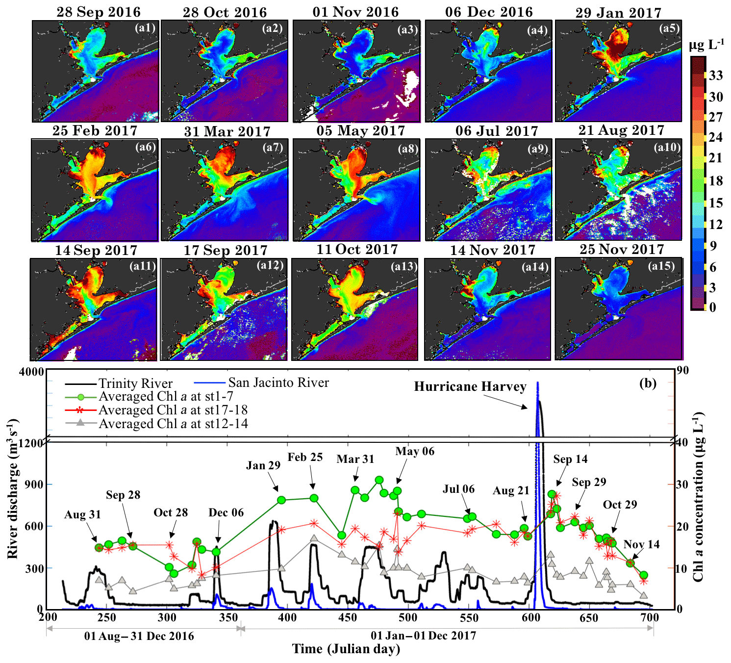
Figure 11(a1−15) OLCI-derived Chl a shown for the period of 31 August 2016–25 November 2017. (b) Trinity River discharge at Romayor, Texas (USGS 08066500; black line), and the west flank of the San Jacinto River (USGS 08067650; blue line); the green, red and gray lines and symbols represent the mean of Chl a at stations 1–7 in Trinity Bay, at stations 17–18 in East Bay and at stations 12–14 close to the entrance of GB corresponding to 43 cloud-free Sentinel-3A OLCI images (colored symbols; dated symbols correspond to images a1−15).
3.2.3 Reconstruction of total pigment absorption spectra from OLCI-derived Chl a
The reconstructed apig(λ) based on the third order function of Chl a_HPLC (gray lines; Fig. 12a and b) agreed well with the spectrophotometrically measured apig(λ) (black lines; Fig. 12a and b) during both surveys (R2=0.86; Fig. 12c). The R2 for modeled versus measured apig(λ) are between 0.76 and 1.00 from 400 to 700 nm with averaged R2 of whole spectra reaching ∼0.82 on 29 September 2017 and ∼0.89 on 29–30 October 2017, respectively. The vector coefficients obtained from Eq. (10) were further applied to Eq. (11) to generate apig_OLCI(λ) based on OLCI-derived Chl a images on 6 July (Fig. 11a9), 29 September (Fig. 10a), 29–30 October (Fig. 10b–c) and 25 November 2017 (Fig. 11a15), respectively; these contained 259×224 pixels in each image. The apig_OLCI(λ) at each pixel was retrieved at 1 nm intervals, and thus 301 images of apig_OLCI(λ) representing each wavelength were obtained over GB.
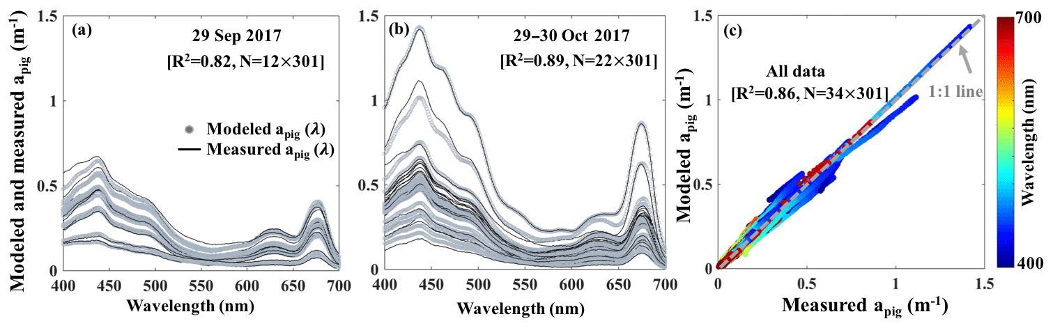
Figure 12Spectrophotometrically measured and multiple-regression fitted apig(λ) spectra acquired on (a) 29 September and (b) 29–30 October 2017 in GB. Gray and black lines represent modeled and measured results, respectively. (c) Comparison between modeled and spectrophotometrically measured apig(λ) for all data with color representing wavelength.
3.2.4 Accuracy of phytoplankton pigment retrievals from Sentinel-3A OLCI
The reconstructed apig_OLCI(λ) was spectrally decomposed into 16 individual pigment spectra at each pixel based on Eq. (13). A comparison of all data between HPLC-measured pigments and NNLS algorithm inverted pigments shows that R2 ranged from a low of 0.40 for diatoxanthin to 0.96 for Chl a, and RMSE was in the range of 0.103–0.584 (Table 4). The NNLS-modeled Chl a also correlated well with OLCI-derived Chl a (R2=0.98; Fig. 13a), with each exhibiting similar quantitative and spatial patterns. For the other 15 simultaneously simulated pigments, R2 of only seven pigments were greater than 0.650 (Table 4). In addition, the resulting RMSEs were less than 0.3 for most of pigments, except zeaxanthin, violaxanthin, diatoxanthin and diadinoxanthin. Further, for those pigments with relatively lower RMSE, their slopes were very close to 1 and y intercepts approached to 0. Five NNLS-derived versus HPLC-measured diagnostic pigments including alloxanthin, Chl b, zeaxanthin, fucoxanthin and peridinin are shown in Fig. 13. The R2 between NNLS-derived and HPLC-measured pigments for surveys 1 and 2 was highest for alloxanthin (0.91; Fig. 13b). For the other pigments R2 was 0.854 for Chl b (Fig. 13c), 0.689 for zeaxanthin (Fig. 13d), 0.645 for fucoxanthin (Fig. 13e) and 0.566 for peridinin (Fig. 13f).
Table 4Statistical results between HPLC-measured and NNLS-modeled pigments.
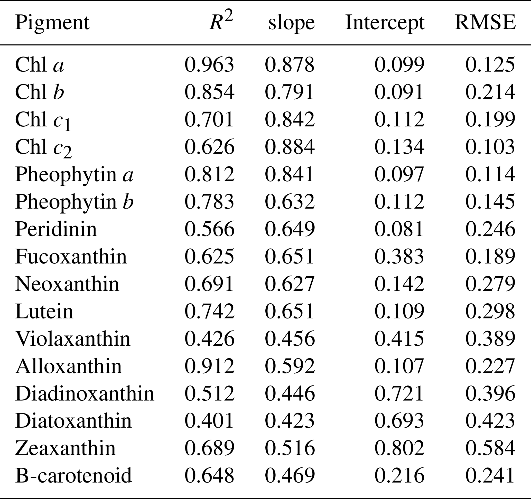

Figure 13Sentinel-3A OLCI-derived pigment concentrations against HPLC-measured pigment concentrations in Galveston Bay: (a) Chl a, (b) alloxanthin, (c) Chl b, (d) zeaxanthin, (e) fucoxanthin and (f) peridinin. Red and green symbols indicate data sets obtained on 29 September and 29–30 October 2017, respectively. The dashed circle includes the station located in algal bloom area.
3.3 Spatiotemporal variations of diagnostic pigments
Flooding due to Hurricane Harvey not only enhanced Chl a but also affected the phytoplankton pigments composition. NNLS-retrieved pigment maps for July, September, October and November 2017 including those of alloxanthin, Chl b, zeaxanthin, fucoxanthin and peridinin (Fig. 14) show different levels of variations before and after the hurricane event. Alloxanthin, which is unique to cryptophytes (Wright and Jeffrey, 2006), exhibited the same spatial distribution patterns (Fig. 14a1–e1) with Chl a. Alloxanthin was especially low (∼0.5 µg L−1, Fig. 14a1) in the major basin area on 6 July 2017 before the hurricane and slightly elevated (∼0.7 µg L−1, Fig. 14b1) in September and October 2017 after the hurricane passage. Furthermore, extremely high alloxanthin (∼3.5 µg L−1, Fig. 14c1–d1) was observed adjacent to San Jacinto River mouth on 29–30 October 2017, which coincided with the high %Chl a of cryptophytes at stations 19 and 23 (Fig. 6b). The bloom with high concentration of alloxanthin on 29 October 2017 (∼3.5 µg L−1; Fig. 14c1) then extended to a broader area on 30 October 2017 (Fig. 14d1).
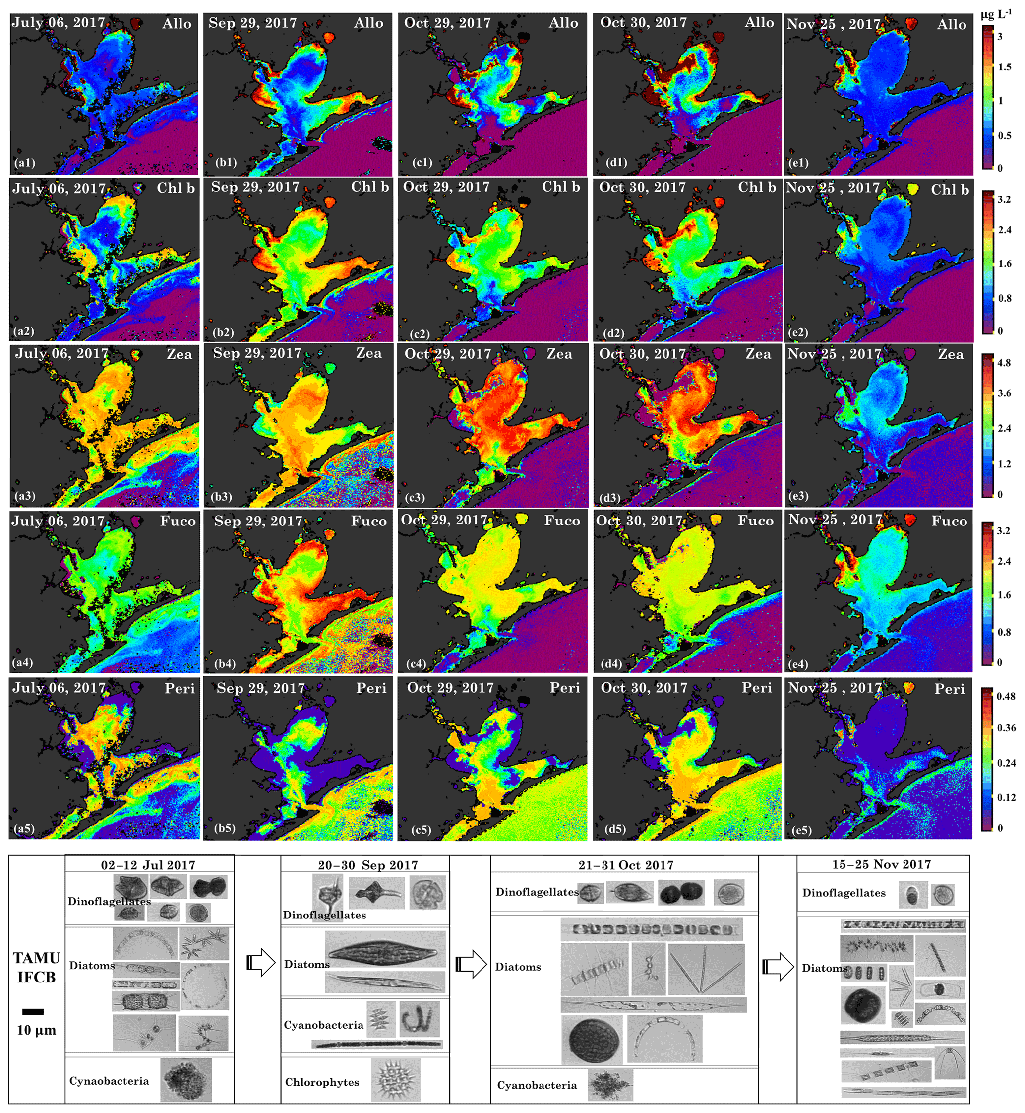
Figure 14Sentinel-3A OLCI-derived maps of diagnostic pigment concentrations for Galveston Bay. Simulated (a1–e1) alloxanthin, (a2–e2) Chl b, (a3–e3) zeaxanthin, (a4–e4) fucoxanthin and (a5–e5) peridinin concentrations. Panels (a), (b), (c), (d) and (e) represent columns (maps for 6 July, 29 September, 29–30 October and 25 November 2017), respectively and panels 1–5 represent rows (pigments). Panels (f), (g), (h) and (l) are the corresponding IFCB data for 6 July, 29 September, 29–30 October and 25 November 2017, respectively. Note that IFCB pictures of freshwater species including chlorophytes and cyanobacteria that appeared on 20–30 September 2017 have been zoomed in for better clarity.
Chl b is abundant in the group of chlorophytes (green algae) (Hirata et al., 2011) and the spatial distributions of Chl b (Fig. 14a2–e2) also showed strong correlations with Chl a on 6 July 2017, 29 September, 29–30 October and 25 November 2017. The NNLS-derived Chl b exhibited overall low values (∼0.5–2 µg L−1; Fig. 14a2) before the hurricane and showed obvious elevation throughout the bay after the hurricane, eventually decreasing to pre-hurricane level by 25 November 2017. Furthermore, Chl b concentrations observed on 29 September 2017 were higher than that on 29–30 October 2017, which corresponded to a decline of the chlorophyte percentage derived from the IOP inversion algorithm (Fig. 6). More importantly, images obtained from IFCB at the entrance to GB also detected a freshwater Chlorophyte species (Pediastrum duplex; Fig. 14g) on 29 September 2017. However, this species was rarely observed in IFCB images for the other dates (Fig. 14a1 and Fig. 14c1–e2). In addition, Chl b concentrations approached ∼2.8 µg L−1 in the bloom area and the corresponding green discoloration of water was also observed during the field survey on 30 October 2017.
Zeaxanthin is known as taxa-specific pigment for prokaryotes (cyanobacteria) (Moisan et al., 2017; Dorado et al., 2015). NNLS-derived zeaxanthin maps (Fig. 14a3–e3) displays significantly different patterns to Chl a concentrations, exhibiting low concentrations in the areas where the Chl a concentrations were high. For example, zeaxanthin was especially low in the bloom area on 29–30 October 2017, which agreed well with low %Chl a of cyanobacteria at stations 19 and 23 (Fig. 6), thus indicating that this localized algal bloom event was not associated with cyanobacteria. In addition, the zeaxanthin concentration was high ∼3.0 µg L−1 (Fig. 14a3) in both GB and shelf waters on July 6 July 2017 before the hurricane event. Later, zeaxanthin increased slightly on 29 September 2017 (Fig. 14b3) with IFCB data detecting N2-fixing cyanobacteria (Anabaena spp.; Fig. 14g) and remained elevated on 29–30 October 2017 (Fig. 14b3–c3). Zeaxanthin eventually decreased to very low values (∼1.2 µg L−1; Fig. 14e3) on 25 November 2017.
Fucoxanthin is a major carotenoid found in diatoms (Hirata et al., 2011; Moisan et al., 2017) and the NNLS-derived fucoxanthin maps (Fig. 14a4–e4) show highly similar distribution patterns with Chl a. Maps of fucoxanthin show low concentrations on 6 July 2017 (∼1.5 µg L−1; Fig. 11a4), and display a large increase on 29 September 2017 (∼1.6–3.0 µg L−1; Fig. 11b4). The diatoms group detected by the IFCB were dominated by marine species before the hurricane but subsequently shifted to freshwater species (e.g., Pleurosigma; Fig. 14g) and then back to marine species after October 2017. Overall, fucoxanthin concentrations in GB were relatively higher during survey 1, which corresponded to the higher %Chl a of diatoms (Fig. 6) compared to survey 2. Although, fucoxanthin decreased to low values on 25 November 2017 (∼1.6 µg L−1; Fig. 11e4), it accounted for a higher fraction of phytoplankton diagnostic pigments compared to other dates in July, September and October 2017.
Peridinin, a primary biomarker pigment for certain dinoflagellates (Örnólfsdóttir et al., 2003), also displayed significantly distinct patterns in comparison to Chl a (Fig. 14a5–e5). On 6 July 2017, peridinin was ∼0.24–0.36 µg L−1, accounting for a high proportion of the diagnostic pigments; meanwhile, diversity of marine dinoflagellate species observed by the IFCB at this time was also high (Fig. 14f). However, peridinin decreased (∼0.001–0.05 µg L−1) after the hurricane, with freshwater dinoflagellate species (Ceratium hirundinella; Fig. 14g) detected by the IFCB on 29 September 2017. In addition, maps of peridinin during both surveys (Fig. 14b5–d5) present a higher concentration (∼0.3 µg L−1) in higher salinity waters adjacent to the bay entrance, which agreed well with the increasing fraction of dinoflagellate at stations 10–14 detected from IOP inversion model (Fig. 6). In contrast, peridinin was found in low concentrations in both GB and shelf waters on 25 November 2017 (Fig. 14e5), with dinoflagellate species rarely observed by the IFCB (Fig. 14l).
4.1 Performance of the semi-analytical IOP inversion algorithm
The residuals between Rrs_insitu and Rrs_mod on 29 September and 29–30 October 2017 are negative in the blue (400–450 nm) and red (610–630 nm) spectral range at most stations, whilst keeping positive ∼700 nm, which could be attributed to a number of factors. First, the underestimation near 700 nm by the IOP inversion model is possibly induced by the absence of a fluorescence component in the IOP inversion model; thus, Rrs_insitu containing fluorescence signals were generally higher than Rrs_mod near 700 nm. Second, in the range of 610–630 nm, the absorption was overestimated at most of the stations; in this spectral range, the shape of spectra was strongly modulated by cyanobacteria absorption. Thus, this overestimation at ∼620 nm is likely introduced by the input absorption spectrum (eigenvector) for cyanobacteria since all of the inputs are general absorption spectral shapes for different phytoplankton groups. However, the spectra of can vary in magnitude and shape associated with package effects under different environmental conditions (e.g., nutrient, light and temperature) even for the same species (Bricaud et al., 2004). More detailed absorption spectra of phytoplankton under different conditions (e.g., high or low light and replete or poor nutrients) could improve the performance of the IOP algorithm. Furthermore, the role of scattering might be another key factor to explain differences between Rrs_insitu and Rrs_mod for the whole spectra. The quantity and composition of suspended materials including phytoplankton, sediment and minerals will collectively determine bbp (λ) in both shape and magnitude. However, the input eigenvector of bbp (λ) in the present study was not divided into detailed sub-constituents and was a sum spectrum-based on a power-law function (Table 2). In reality, bbp (λ) spectra are not smooth and regular, and thus the bbp (λ) values of phytoplankton and sediment might introduce errors to the whole spectrum due to their own scattering characteristics.
4.2 Distributions of NNLS-retrieved phytoplankton pigments from Sentinel-3A OLCI
The NNLS-inversion algorithm showed relatively higher R2 for those pigments that better correlated with HPLC-measured Chl a (e.g., Chl b and alloxanthin), which was reasonably consistent with Moisan et al. (2017). This outcome could potentially be attributed to the fact that the NNLS-pigment inversion algorithm was developed based on the relationship between HPLC-measured Chl a and spectrophotometer-measured apig(λ). For instance, pigments that were relatively poorly correlated with HPLC-measured Chl a, such as fucoxanthin, diatoxanthin and diadinoxanthin on 29–30 October 2017, the OLCI-derived concentrations in the cryptophyte–chlorophyte algal bloom area showed higher concentrations than those of HPLC measurements (e.g., values in gray circle; Fig. 13e), thus resulting in lower R2. However in previous studies (Moisan et al., 2017; Pan et al., 2010), relatively higher R2 versus lower RMSE were observed between satellite-derived and HPLC-measured fucoxanthin compared to this study. This was likely because in addition to being based on long-term measurements, fucoxanthin is one of the most abundant diatom biomarker pigments in coastal waters and correlated very well with Chl a in their study area (United States northeast coast). In contrast, the cryptophyte–chlorophyte algal bloom area with extremely high Chl a appeared to disturb the correlations between Chl a and fucoxanthin in this study. Also, pigments with apparent high values in algal bloom areas, such as Chl b, Chl c, alloxanthin, lutein, showed higher R2 with RMSE less than 0.3. Thus, in situ measurements of Chl a and apig(λ) in waters with stronger gradients in magnitude and greater variations in phytoplankton community structures could potentially increase the challenge of applying NNLS-inversion algorithms in optically complex estuarine waters. Further, the highly dynamic estuarine environment could contribute as well to additional uncertainties in the validation of inverted pigments due to variations such as turbulence, turbidity or light field that are likely to occur during the time interval between in situ and Sentinel-3 OLCI (∼4 h) observations. HPLC measurements also cannot detect extremely low pigment concentrations; for example, HPLC-measured peridinin concentrations were 0.001 µg L−1 at several stations, however, OLCI-derived peridinin showed higher and variable values at these stations (data in gray circles; Fig. 13f), thus this could increase the RMSE of the NNLS-inverted peridinin. It was also found that the slopes of all pigments were smaller than 1, which demonstrate that NNLS-inverted pigments were relatively smaller than HPLC measurements, especially for those stations located in the algal bloom area; this could most likely be attributed to the underestimation of Chl a values by the Sentinel-3 OLCI empirical algorithms in the algal bloom area. Algal bloom dominated by the cryptophytes group, which is also known to cause red tides worldwide, to some degree, could increase red reflectance and thus increase ratio values of red ∕ NIR and decrease estimated Chl a values. Therefore, reliable estimates of satellite-detected Chl a is crucial for the accuracy of retrieved pigments. The goal of the empirical Chl a algorithm for Sentinel-3A OLCI is to obtain a more accurate estimation of surface Chl a concentration, which is better for retrieving other accessory pigments. However, the primary limitation of Chl a empirical algorithms in this study was that the derived relationships between red ∕ NIR and Chl a in GB may only be valid within a specific time period due to temporally limited field observations versus highly dynamic estuarine environments. Therefore, a Chl a empirical algorithm that is more broadly applicable over a longer time period will largely improve the accuracy of retrieved pigments over a series of remote-sensing images and can be more useful for spatiotemporal studies of phytoplankton functional diversity. More importantly, the highly similar absorption spectra of many carotenoids are another key issue limiting the accuracy of spectral decomposition techniques. Although the 16 input pigment spectra used in this study were selected from Thrane et al., 2015), which were correctly identified from unknown phytoplankton community structure with low error rate reported from Monte Carlo tests, the potential effects of aliasing spectra of some pigment pairs (e.g., fucoxanthin vs. peridinin, diadinoxanthin vs. lutein, β-carotene vs. zeaxanthin) could still be a factor. Thus, the reported errors or R2 for the retrieved total carotenoids in Thrane et al. (2015) were apparently lower or higher, respectively, than those of modeled total chlorophylls, which showed consistency with this study. Although the predicted pigments showed a range of R2 and RMSE with known uncertainties, all are within the acceptable range and could be useful for studying the spatiotemporal responses of PFTs to environmental variations, especially in such optically complex estuaries.
The derived maps of phytoplankton diagnostic pigments appeared to be reasonably correlated with HPLC-measured diagnostic pigments and showed overall agreement with extracted phytoplankton taxonomic compositions detected from the IOP inversion algorithm. The retrieved diatom-specific fucoxanthin maps, however, show high concentrations compared to other pigments adjacent to the entrance (Fig. 13b4 and c4), which contradicts the diatom %Chl a calculated from the IOP inversion algorithm. As the Chl a fraction of diatoms was relatively uniform at stations 12–14 (Fig. 6b) Nair et al.(2008) concluded that fucoxanthin can occur in other phytoplankton types (e.g., raphidophyte and haptophyte). Fucoxanthin and/or fucoxanthin derivatives such as 19′-hexanoyloxyfucoxanthin can also replace peridinin as the major carotenoid in some dinoflagellates (e.g., Karenia brevis; Jeffrey and Vest, 1997). The elevated contributions from groups of dinoflagellates, haptophytes and prochlorophytes adjacent to the entrance (stations 10–14; Fig. 6b) along with high concentrations of fucoxanthin likely suggest the presence of elevated fractions of haptophytes and dinoflagellates, and further implies that fucoxanthin is an ambiguous marker pigment for diatoms. This could also explain the poor correlation between inverted %Chl a and %DP observed for the groups of diatoms and haptophytes (Fig. 4g and l). These results also further suggest the inherent limitations of using a DP-type comparison between major biomarker pigments and phytoplankton groups because the major assumption for DP-type methods is that the diagnostic pigment of distinct phytoplankton groups are uncorrelated to each other. This assumption is invalid in that concentrations of major biomarker pigments are significantly correlated with each other and also may vary in time and space under some external environmental stress (e.g., temperature, salinity, mixing, light and nutrient) (Latasa and Bidigare, 1998).
4.3 Response of phytoplankton taxa to environmental conditions
Previous studies showed diatoms to be the most abundant taxa in GB, and they tend to be more dominant during winter and spring, corresponding to periods of high freshwater discharge and nutrient-replete conditions (Dorado et al., 2015; Örnólfsdóttir et al., 2004a). Transitions from chain-forming diatoms such as Chaetoceros and rod-like diatoms pre-flood to small cells, such as Thalassiosira and small pennate diatoms were generally observed during high-river discharge periods (Anglès et al., 2015; Lee, 2017). In contrast, cyanobacteria were the most abundant species during the warmer months (June–August) when river discharge was relatively low (Örnólfsdóttir et al., 2004b). Further, phytoplankton groups in GB responded differentially both taxonomically and spatially to the freshening events due to their contrasting nutrient requirements and specific growth characteristics. For instance, most phytoplankton taxa (e.g., diatom, chlorophyte and cryptophyte) can be positively stimulated by fresh inflows due to their relatively rapid growth rate (Paerl et al., 2003). However, Roelke et al. (2013) also documented that cyanobacteria and haptophytes in the upper GB were not sensitive to nutrient-rich waters from both rivers due to the extra nutrients obtained from N2-fixation abilities and mixotrophic characteristics, respectively. In the lower part of GB, dinoflagellates and cyanobacteria are known to be more dominant during the low-river discharge due to their preference for higher phosphorus (P) compared to some other groups, and to low turbulence (Lee, 2017), and thus are generally inversely related to the fresh inflows (Lee, 2017; Roelke et al., 2013).
Perturbations following Hurricane Harvey affected the phytoplankton taxonomic composition with alterations in phytoplankton community structure observed as the GB system transitioned from marine to freshwater then to marine system (Figs. 6 and 14). Higher fractions of zeaxanthin and peridinin and the presence of large and slow-growing marine dinoflagellates detected by the IFCB pre-hurricane (6 July 2017) indicate that both cyanobacteria and dinoflagellates were the main groups of the phytoplankton community during summer, and were likely associated with warmer temperature and lower river flow (Lee, 2017). Later, massive Chl a observed in September 2017 and the decline of Chl a to background state in October 2017 were likely associated with the hurricane-induced high-river discharge and the resulting variations in nutrient concentration and composition. Higher fractions of diatoms and chlorophytes accompanied by increasing fucoxanthin and Chl b on 29 September 2017 to some extent agreed well with measurements of Steichen et al. (2018) in the two weeks following Hurricane Harvey that freshwater species (diatoms, green algae and cyanobacteria) appeared immediately following the flooding event. The greater abundance of diatoms and chlorophytes during survey 1 in comparison to survey 2 were likely due to their rapid growth rates, enhanced nutrient uptake rates, and tolerance of low salinity and high turbulence under high nutrient loading conditions following the freshwater inflows (Roy et al., 2013; Santschi, 1995). Therefore, it is not surprising that Chl b concentrations showed very low values in July and November, 2017, when river discharge was correspondingly low. Cyanobacteria, which normally prefer low salinity conditions, also showed specific responses to this flood event. On 29 September 2017, zeaxanthin slightly increased compared to summer season in July 2017. The decline of diatoms and chlorophytes versus slightly increased cyanobacteria levels observed on 29–30 October 2017 could be attributed to the relatively slow growth rates of cyanobacteria compared to that of chlorophytes and diatoms (Paerl et al., 2003); cyanobacteria appeared to have lagged behind these groups in terms of responding to enhanced freshwater discharge when longer residence times were again restored. In contrast, the presence of green algae and cyanobacteria could as well be explained by the clarity and turbidity gradient of water. Quigg et al. (2010) reported that when turbidity was relatively high, chlorophytes dominated over cyanobacteria with biomass ratio of chlorophyte/cyanobacteria greater than two, which supported our observations that chlorophyte dropped off whilst cyanobacteria increased during survey 2 on 29–30 October 2017. In addition the highest cyanobacteria percentage in East Bay suggests that calm and stratified waters may accelerate cyanobacteria growth as the buoyancy regulation mechanism of cyanobacteria is possibly restricted by the water mixing (Roy et al., 2013). The peridinin concentration, which initially decreased in September and then increased in the lower GB on 29–30 October 2017, suggests that dinoflagellates show overall preference for high-salinity waters. Furthermore, previous IFCB observations from Biological and Chemical Oceanography Data Management Office (BCO-DMO) showed that algal blooms after hurricanes in the nGOM were initially dominated by diatoms, and subsequently transitioned to blooms of dinoflagellates, likely associated with nutrient ratios and chemical forms of nutrients supplied by the flood waters and rainfall (Heisler et al., 2008). In addition, high concentrations of peridinin observed along the Houston Ship Channel might provide evidence that the ballast water addition from shipping vessels likely promotes harmful species of dinoflagellates (Steichen et al., 2015). Finally, low concentrations of all pigments on 25 November 2017 with relatively higher fractions of fucoxanthin compared to previous dates (Fig. 14), indicate the major role of marine diatoms at that time and further confirms that diatoms can be found under a wide range of inflows in GB.
The localized cryptophyte–chlorophyte bloom that occurred ∼60 d after Hurricane Harvey on 29–30 October 2017 was captured by both satellite and in situ measurements. This bloom might not be associated with the flooding events of Hurricane Harvey, and could be linked to nutrient-rich runoff flowing into GB, reflecting the sensitivity and rapid response of the phytoplankton community to nutrient input in GB. In shallow and turbid estuaries, human activities are altering the environment and causing phytoplankton changes in diversity and biomass to occur more frequently. Dugdale et al. (2012) reported that variations of the phytoplankton community in the San Francisco estuary could be attributed to anthropogenically elevated concentration of ammonium, which restrains the uptake of nitrate, thus reducing the growth and reproduction of larger diatoms and shifting towards smaller species (e.g., cryptophytes and green flagellates). Furthermore, “pink oyster” events related to alloxanthin of cryptophytes in GB occurred more frequently from September through October in recent years (Paerl et al., 2003). The eastern side of the Houston Ship Channel in the mid-bay region was reported as the area most heavily impacted by the intense “pink oyster” events. Previous studies and present observations both suggest that this cryptophyte–chlorophyte-dominated bloom could be promoted by the nutrient-driven eutrophication from the Houston Ship Channel, urbanization and industrialization along the upper San Jacinto River complex.
4.4 Photo-physiological state of natural phytoplankton community
In this study, the CDOM-corrected Fv∕Fm and σPSII likely represented a composite of both phytoplankton taxonomy and physiological stress (e.g., nutrient and mixing). Typically, lowest N and P concentrations were measured closest to the nGOM (Quigg et al., 2009). Phytoplankton communities living close to nGOM were usually in poor nutrient conditions and would have been expected to maximize their light harvesting (increase in σPSII) due to nutrient stress. Simultaneously, phytoplankton cells might experience a decline of functional proportion of reaction centers of PSII (RCII), which means a decrease in Fv∕Fm. The observed low levels of Fv∕Fm and Chl a ∕ TP versus high values of σPSII and AP ∕ TP adjacent to the nGOM showed agreement with previous studies that the fraction of carotenoids is higher for nutrient-poor cultures (Schitüter et al., 1997; Holmboe et al., 1999). In contrast, phytoplankton in well-mixed waters (stations 7–9) might experience abundant nutrients due to the resuspension of the cyclonic gyre around Smith Point; as such, their photosynthetic machinery were likely healthier. Aiken et al. (2004) documented that the Chl a ∕ TP ratio was relatively higher when plants were in good growing conditions, which is similar to the observations in this study that phytoplankton have a higher fraction of Chl a accompanying higher rate of photosynthetic efficiency (Fv∕Fm) under nutrient replete conditions. Overall, the spatial pattern of Fv∕Fm and σPSII in GB could be mainly attributed to physiological stress of nutrient and hydrodynamic conditions since the light availability (PAR) during the sampling period did not spatially vary significantly at the surface. Furthermore, FIRe measurements (Fv∕Fm and σPSII) also presented a taxonomic signal superimposed upon environmental factors. Each cluster with different dominant taxa (well-mixed group, chlorophyte–cryptophyte, cyanobacteria and dinoflagellate–haptophyte) displayed different physiological characteristics. The taxonomic sequence of eukaryotic groups from high Fv∕Fm, low σPSII to low Fv∕Fm, high σPSII in the present observations showed potential effects of phytoplankton cell size corresponding to diatoms, chlorophytes, cryptophytes, dinoflagellates and haptophytes. The prokaryote (cyanobacteria) had relatively high values of Fv∕Fm and low values of σPSII; this agreed with Fv∕Fm for some species of nitrogen-fixing cyanobacteria that can range from 0.6 to 0.65 (Berman-Frank et al., 2007). Yet, it is difficult to separate the contributions from environmental factors and taxonomic variations to the changes of FIRe fluorescence signals since all these parameters are interrelated. Different phytoplankton groups and sizes will display distinct physiological traits (Fv∕Fm and σPSII) when experiencing considerable environmental pressures. Thus, effects of physiological stress on Fv∕Fm and σPSII variations for natural samples can only be determined when taxonomic composition can be excluded as a contributor (Suggett et al., 2009).
Field measurements (salinity, pigments, optical properties and physiological parameters) and ocean color observations from Sentinel-3A OLCI were used to study the effects of extreme flooding associated with Hurricane Harvey on the phytoplankton community structures, pigment distributions and their physiological state in GB. Flooding effects made the entire GB transition from saline to freshwater then back to a more marine-influenced system. The band ratio (red ∕ NIR) of Rrs_insitu were negatively correlated with HPLC-measured Chl a in an exponential relationship (R2>0.93). The satellite-retrieved Chl a maps yielded much higher Chl a concentrations on 29 September 2017 compared to 29–30 October 2017 with lowest Chl a observed adjacent to the shelf waters. The phytoplankton taxonomic composition was further retrieved from Rrs_insitu using a 10-species IOP inversion algorithm. The phytoplankton community generally dominated by estuarine marine diatoms and dinoflagellates before flood events, was altered to freshwater species of diatoms, green algae (chlorophytes) and cyanobacteria during survey 1. It also showed an increase of small-size species including cryptophytes, haptophytes, prochlorophytes and cyanobacteria accompanied by a decline of chlorophytes and diatoms during survey 2.
Phytoplankton diagnostic pigments retrieved using an NNLS inversion model based on Sentinel-3A OLCI Chl a maps also confirmed spatiotemporal variations of phytoplankton taxonomy. The NNLS-retrieved diagnostic pigment maps showed overall spatiotemporal agreement with HPLC measurements with R2 ranging from 0.40 (diatoxanthin) to 0.96 (Chl a) during both surveys. Alloxanthin, Chl b and fucoxanthin, which exhibited similar patterns with Chl a, showed different levels of increase after Hurricane Harvey. In contrast, NNLS-derived zeaxanthin and peridinin presented significantly low values in the area where Chl a concentrations were high. Further, maps of zeaxanthin and peridinin display relatively higher fractions on 6 July 2017 before the hurricane compared to other diagnostic pigments. However, the peridinin concentration decreased post-hurricane on 29 September 2017 and then increased a bit on 29–30 October 2017. Concentrations of Chl a and all biomarker pigments eventually decreased to low levels in November 2017 when GB returned to its typical environmental state.
Finally, the retrieved phytoplankton taxonomic compositions from the IOP inversion algorithm were linked with FIRe-measured photosynthetic parameters (Fv∕Fm and σPSII) to assess the effects of physiological stress and taxonomic contributions on phytoplankton photosynthetic performance. An inverse relationship between the Fv∕Fm and σPSII were observed during both surveys. The phytoplankton community in well-mixed waters (around Smith Point) showed high Fv∕Fm against low σPSII; in contrast, the area with poor nutrient conditions (adjacent to the shelf waters) showed low Fv∕Fm and elevated σPSII. Taxonomic signatures of Fv∕Fm and σPSII revealed diverse physiological characteristics with dinoflagellate–haptophyte group showing the lowest Fv∕Fm versus the highest σPSII, whereas prokaryotes of the cyanobacteria-dominated group showed high values of Fv∕Fm and low values of σPSII. Overall, this study using field and ocean color data combined with inversion algorithms provided novel insights on phytoplankton response to an extreme flood perturbation in a turbid estuarine environment based on taxonomy, pigment composition and physiological state of phytoplankton.
Data from field measurements are available upon request from the corresponding author.
BL and ED conceived and designed the research; BL, ED and IJ collected and processed the data; BL analyzed the data and all authors contributed to writing the paper.
The authors declare that they have no conflict of interest.
The authors thank the European Space Agency (ESA) and the European Organization for the Exploitation of Meteorological Satellites (EUMETSAT) for providing access to the Sentinel-3 OLCI ocean color data and the Sentinel-3 Toolbox Kit Module (S3TBX) version 5.0.1 in the Sentinel Application Platform (SNAP). We also would like to thank the Phytoplankton Dynamics Lab of Texas A&M University at Galveston for the near-real-time microplankton pictures recorded by an Imaging FlowCytobot, which are made available on the web. We are grateful to Bill Gibson from the Coastal Studies Institute, Louisiana State University, for providing logistic support for field operations. Eurico D'Sa acknowledges NASA support through grant no. 80NSSC18K0177.
This paper was edited by Maria Tzortziou and reviewed by two anonymous referees.
Acker, J., Lyon, P., Hoge, F., Shen, S., Roffer, M., and Gawlikowski, G.: Interaction of Hurricane Katrina with optically complex water in the Gulf of Mexico: interpretation using satellite-derived inherent optical properties and chlorophyll concentration, IEEE Geosci. Remote S., 6, 209–213, 2009.
Aiken, J., Fishwick, J., Moore, G., and Pemberton, K.: The annual cycle of phytoplankton photosynthetic quantum efficiency, pigment composition and optical properties in the western English Channel, J. Mar. Biol. Assoc. UK, 84, 301–313, 2004.
Alvain, S., Moulin, C., Dandonneau, Y., and Bréon, F.-M.: Remote sensing of phytoplankton groups in case 1 waters from global SeaWiFS imagery, Deep-Sea Res. Pt. I, 52, 1989–2004, 2005.
Anglès, S., Jordi, A., and Campbell, L.: Responses of the coastal phytoplankton community to tropical cyclones revealed by high-frequency imaging flow cytometry, Limnol. Oceanogr., 60, 1562–1576, 2015.
Barlow, R., Cummings, D., and Gibb, S.: Improved resolution of mono-and divinyl chlorophylls a and b and zeaxanthin and lutein in phytoplankton extracts using reverse phase C-8 HPLC, Mar. Ecol. Progr. Ser., 161, 303–307, 1997.
Behrenfeld, M. J. and Falkowski, P. G.: Photosynthetic rates derived from satellite-based chlorophyll concentration, Limnol. Oceanogr., 42, 1–20, 1997.
Behrenfeld, M. J. and Kolber, Z. S.: Widespread iron limitation of phytoplankton in the South Pacific Ocean, Science, 283, 840–843, 1999.
Berman-Frank, I., Quigg, A., Finkel, Z. V., Irwin, A. J., and Haramaty, L.: Nitrogen-fixation strategies and Fe requirements in cyanobacteria, Limnol. Oceanogr., 52, 2260–2269, 2007.
Bidigare, R. R., Ondrusek, M. E., Morrow, J. H., and Kiefer, D. A.: In-vivo absorption properties of algal pigments, Ocean Optics X, Intl. Soc. Opt. Photonics., 1302, 290–303, 1990.
Blondeau-Patissier, D., Gower, J. F., Dekker, A. G., Phinn, S. R., and Brando, V. E.: A review of ocean color remote sensing methods and statistical techniques for the detection, mapping and analysis of phytoplankton blooms in coastal and open oceans, Progr. Oceanogr., 123, 123–144, 2014.
Bracher, A., Taylor, M. H., Taylor, B., Dinter, T., Röttgers, R., and Steinmetz, F.: Using empirical orthogonal functions derived from remote-sensing reflectance for the prediction of phytoplankton pigment concentrations, Ocean Sci., 11, 139–158, https://doi.org/10.5194/os-11-139-2015, 2015.
Brewin, R. J., Sathyendranath, S., Hirata, T., Lavender, S. J., Barciela, R. M., and Hardman-Mountford, N. J.: A three-component model of phytoplankton size class for the Atlantic Ocean, Ecol. Modell., 221, 1472–1483, 2010.
Bricaud, A., Claustre, H., Ras, J., and Oubelkheir, K.: Natural variability of phytoplanktonic absorption in oceanic waters: Influence of the size structure of algal populations, J. Geophys. Res.-Oceans, 109, C11010, https://doi.org/10.1029/2004JC002419, 2004.
Campbell, D., Hurry, V., Clarke, A. K., Gustafsson, P., and Öquist, G.: Chlorophyll fluorescence analysis of cyanobacterial photosynthesis and acclimation, Microbiol. Molecul. Biol. Rev., 62, 667–683, 1988.
Carder, K. L., Chen, F., Lee, Z., Hawes, S., and Kamykowski, D.: Semianalytic Moderate-Resolution Imaging Spectrometer algorithms for chlorophyll a and absorption with bio-optical domains based on nitrate-depletion temperatures, J. Geophys. Res.-Oceans, 104, 5403–5421, 1999.
Chase, A., Boss, E., Zaneveld, R., Bricaud, A., Claustre, H., Ras, J., Dall'Olmo, G., and Westberry, T. K.: Decomposition of in situ particulate absorption spectra, Meth. Oceanogr., 7, 110–124, 2013.
Chase, A., Boss, E., Cetinić, I., and Slade, W.: Estimation of phytoplankton accessory pigments from hyperspectral reflectance spectra: toward a global algorithm, J. Geophys. Res.-Oceans, 122, 9725–9743, 2017.
Ciotti, A. M., Lewis, M. R., and Cullen, J. J.: Assessment of the relationships between dominant cell size in natural phytoplankton communities and the spectral shape of the absorption coefficient, Limnol. Oceanogr., 47, 404–417, 2002.
Cullen, J. J. and Davis, R. F.: The blank can make a big difference in oceanographic measurements, Limnol. Oceanogr., 12, 29–35, 2003.
D'Sa, E. J.: Assessment of chlorophyll variability along the Louisiana coast using multi-satellite data, GISci. Remote Sens., 51, 139–157, 2014.
D'Sa, E. J. and Lohrenz, S. E.: Theoretical treatment of fluorescence detection by a dual-fiber-optic sensor with consideration of sampling variability and package effects associated with particles, Appl. Optics, 38, 2524–2535, 1999.
D'Sa, E. J., Lohrenz, S. E., Asper, V. L., and Walters, R. A.: Time series measurements of chlorophyll fluorescence in the oceanic bottom boundary layer with a multisensor fiber-optic fluorometer, J. Atmos. Ocean. Technol., 14, 889–896, 1997.
D'Sa, E. J., Miller, R. L., and Del Castillo, C.: Bio-optical properties and ocean color algorithms for coastal waters influenced by the Mississippi River during a cold front, Appl. Optics, 45, 7410–7428, 2006.
D'Sa, E. J., Korobkin, M., and Ko, D. S.: Effects of Hurricane Ike on the Louisiana–Texas coast from satellite and model data, Remote Sens. Lett., 2, 11–19, 2011.
D'Sa, E. J., Joshi, I., and Liu, B.: Galveston Bay and coastal ocean optical-geochemical response to Hurricane Harvey from VIIRS ocean color, Geophys. Res. Lett., 45, 10579–10589, https://doi.org/10.1029/2018GL079954, 2018.
Devred, E., Sathyendranath, S., Stuart, V., and Platt, T.: A three component classification of phytoplankton absorption spectra: Application to ocean-color data, Remote Sens. Environ., 115, 2255–2266, 2011.
Dierssen, H. M., Kudela, R. M., Ryan, J. P., and Zimmerman, R. C.: Red and black tides: Quantitative analysis of water-leaving radiance and perceived color for phytoplankton, colored dissolved organic matter, and suspended sediments, Limnol. Oceanogr., 51, 2646–2659, 2006.
Doerffer, R. and Schiller, H.: The MERIS Case 2 water algorithm, Intl. J. Remote Sens., 28, 517–535, 2007.
Dorado, S., Booe, T., Steichen, J., McInnes, A. S., Windham, R., Shepard, A., Lucchese, A. E., Preischel, H., Pinckney, J. L., and Davis, S. E.: Towards an understanding of the interactions between freshwater inflows and phytoplankton communities in a subtropical estuary in the Gulf of Mexico, PLoS One, 10, e0130931, https://doi.org/10.1371/journal.pone.0130931, 2015.
Dugdale, R., Wilkerson, F., Parker, A. E., Marchi, A., and Taberski, K.: River flow and ammonium discharge determine spring phytoplankton blooms in an urbanized estuary, Estuar. Coast. Shelf Sci., 115, 187–199, 2012.
Dutkiewicz, S., Hickman, A. E., Jahn, O., Gregg, W. W., Mouw, C. B., and Follows, M. J.: Capturing optically important constituents and properties in a marine biogeochemical and ecosystem model, Biogeosciences, 12, 4447–4481, https://doi.org/10.5194/bg-12-4447-2015, 2015.
Farfan, L. M., D'Sa, E. J., and Liu, K.: Tropical cyclone impacts on coastal regions: the case of the Yucatan and the Baja California Peninsulas, Mexico, Estuar. Coast., 37, 1388–1402, 2014.
Ficek, D., Kaczmarek, S. A., Stoñ-Egiert, J., Wozniak, B., Majchrowski, R., and Dera, J.: Spectra of light absorption by phytoplankton pigments in the Baltic; conclusions to be drawn from a Gaussian analysis of empirical data, Oceanologia, 46, 533–555, 2004.
Fishwick, J. R., Aiken, J., Barlow, R., Sessions, H., Bernard, S., and Ras, J.: Functional relationships and bio-optical properties derived from phytoplankton pigments, optical and photosynthetic parameters; a case study of the Benguela ecosystem, J. Mar. Biol. Assoc. UK, 86, 1267–1280, 2006.
Garver, S. A. and Siegel, D. A.: Inherent optical property inversion of ocean color spectra and its biogeochemical interpretation: 1. Time series from the Sargasso Sea, J. Geophys. Res.-Oceans, 102, 18607–18625, 1997.
Geider, R. J., La Roche, J., Greene, R. M., and Olaizola, M.: Response of the photosynthetic apparatus of phaeodactylum tricornutum (bacillariophyceae to nitrate, phosphate, or iron starvation, J. Phycol., 29, 755–766, 1993.
Gilerson, A. A., Gitelson, A. A., Zhou, J., Gurlin, D., Moses, W., Ioannou, I., and Ahmed, S. A.: Algorithms for remote estimation of chlorophyll-a in coastal and inland waters using red and near infrared bands, Opt. Express, 18, 24109–24125, 2010.
Gitelson, A.: The peak near 700 nm on radiance spectra of algae and water: relationships of its magnitude and position with chlorophyll concentration, Int. J. Remote Sens., 13, 3367–3373, 1992.
Gordon, H. R., Brown, O. B., Evans, R. H., Brown, J. W., Smith, R. C., Baker, K. S., and Clark, D. K.: A semianalytic radiance model of ocean color, J. Geophys. Res.-Atmos., 93, 10909–10924, 1988.
Guthrie, C. G., Matsumoto, J., and Solis, R.: Analysis of the influence of water plan strategies on inflows and salinity in Galveston Bay, Final report to the United States Army Corps of Engineers, Contract #R0100010015, Texas Water Development Board, Austin, Texas, USA, 71 pp., 2012.
Heisler, J., Glibert, P. M., Burkholder, J. M., Anderson, D. M., Cochlan, W., Dennison, W. C., and Lewitus, A.: Eutrophication and harmful algal blooms: a scientific consensus, Harmful Algae, 8, 3–13, 2008.
Hirata, T., Aiken, J., Hardman-Mountford, N., Smyth, T. J., and. Barlow, R. G.: An absorption model to determine phytoplankton size classes from satellite ocean colour, Remote Sens. Environ., 112, 3153–3159, 2008.
Hirata, T., Hardman-Mountford, N. J., Brewin, R. J. W., Aiken, J., Barlow, R., Suzuki, K., Isada, T., Howell, E., Hashioka, T., Noguchi-Aita, M., and Yamanaka, Y.: Synoptic relationships between surface Chlorophyll-a and diagnostic pigments specific to phytoplankton functional types, Biogeosciences, 8, 311–327, https://doi.org/10.5194/bg-8-311-2011, 2011.
Hoepffner, N. and Sathyendranath, S.: Effect of pigment composition on absorption properties of phytoplankton, Mar. Ecol. Progr. Ser., 73, l–23, 1991.
Hoge, F. E. and Lyon, P. E.: Satellite retrieval of inherent optical properties by linear matrix inversion of oceanic radiance models: an analysis of model and radiance measurement errors, J. Geophys. Res.-Oceans, 101, 16631–16648, 1996.
Holmboe, N., Jensen, H. S., and Andersen, F. Ø.: Nutrient addition bioassays as indicators of nutrient limitation of phytoplankton in a eutrophic estuary, Mar. Ecol. Progr. Ser., 186, 95–104, 1999.
Howarth, R. W., Marino, R., Lane, J., and Cole, J. J.: Nitrogen fixation in freshwater, estuarine, and marine ecosystems, 1. Rates and importance, Limnol. Oceanogr., 33, 669–687, 1988.
Hu, C., and Feng, L.: Modified MODIS fluorescence line height data product to improve image interpretation for red tide monitoring in the eastern Gulf of Mexico, J. Appl. Remote Sens., 11, 012003, https://doi.org/10.1117/1.JRS.11.012003, 2016.
Hu, C., Cannizzaro, J., Carder, K. L., Muller-Karger, F. E., and Hardy, R.: Remote detection of Trichodesmium blooms in optically complex coastal waters: Examples with MODIS full-spectral data, Remote Sens. Environ., 114, 2048–2058, 2010.
Jeffrey, S. and Vest, M.: Introduction to marine phytoplankton and their pigment signatures, in: Phytoplankton pigment in oceanography, edited by: Jeffrey, S. W., Mantoura, R. F. C., and Wright, S. W., UNESCO Publishing, Paris, France, 37–84, 1997.
Joshi, I. D. and D'Sa, E. J.: Seasonal variation of colored dissolved organic matter in Barataria Bay, Louisiana, using combined Landsat and field data, Remote Sens., 7, 12478–12502, 2015.
Joshi, I. D. and D'Sa, E. J.: An estuarine-tuned quasi-analytical algorithm (QAA-V): assessment and application to satellite estimates of SPM in Galveston Bay following Hurricane Harvey, Biogeosciences, 15, 4065–4086, https://doi.org/10.5194/bg-15-4065-2018, 2018.
Joshi, I. D., D'Sa, E. J., Osburn, C. L., Bianchi, T. S., Ko, D. S., Oviedo-Vargas, D., Arellano, A. R., and Ward, N. D.: Assessing chromophoric dissolved organic matter (CDOM) distribution, stocks, and fluxes in Apalachicola Bay using combined field, VIIRS ocean color, and model observations, Remote Sens. Environ., 191, 359–372, 2017.
Kolber, Z. S., Zehr, J., and Falkowski, P. G.: Effects of growth irradiance and nitrogen limitation on photosynthetic energy conversion in photosystem II, Plant Physiol., 88, 923–929, 1988.
Kolber, Z. S., Prášil, O., and Falkowski, P. G.: Measurements of variable chlorophyll fluorescence using fast repetition rate techniques: defining methodology and experimental protocols, BBA-Bioenergetics, 1367, 88–106, 1998.
Latasa, M. and Bidigare, R. R.: A comparison of phytoplankton populations of the Arabian Sea during the Spring Intermonsoon and Southwest Monsoon of 1995 as described by HPLC-analyzed pigments, Deep-Sea Res. Pt. II, 45, 2133–2170, 1998.
Lee, Z., Carder, K. L., Peacock, T., Davis, C., and Mueller, J.: Method to derive ocean absorption coefficients from remote-sensing reflectance, Appl. Optics, 35, 453–462, 1996.
Lee, Z., Carder, K. L., and Arnone, R. A.: Deriving inherent optical properties from water color: a multiband quasi-analytical algorithm for optically deep waters, Appl. Optics, 41, 5755–5772, 2002.
Lee, H. A.: Effects of Physical Disturbance on Phytoplankton Diversity and Community Composition in Galveston Bay, TX, during an Extreme Flooding Event, Master's thesis, Texas A & M University, available at http://hdl.handle.net/1969.1/161576 (last access: 29 April 2019), 2017.
Lohrenz, S. E., Weidemann, A. D., and Tuel, M.: Phytoplankton spectral absorption as influenced by community size structure and pigment composition, J. Plankton Res., 25, 35–61, 2003.
Lutz, V. A., Sathyendaranath, S., Head, E. J., and Li, W. K.: Changes in the in vivo absorption and fluorescence excitation spectra with growth irradiance in three species of phytoplankton, J. Plankton Res., 23, 555–569, 2001.
Mackey, M., Mackey, D., Higgins, H., and Wright, S.: CHEMTAX-a program for estimating class abundances from chemical markers: application to HPLC measurements of phytoplankton, Mar. Ecol. Progr. Ser., 144, 265–283, 1996.
Maritorena, S., Siegel, D. A., and Peterson, A. R.: Optimization of a semianalytical ocean color model for global-scale applications, Appl. Optics, 41, 2705–2714, 2002.
Moisan, T. A., Moisan, J. R., Linkswiler, M. A., and Steinhardt, R. A.: Algorithm development for predicting biodiversity based on phytoplankton absorption, Cont. Shelf Res., 55, 17–28, 2013.
Moisan, T. A., Rufty, K. M., Moisan, J. R., and Linkswiler, M. A.: Satellite observations of phytoplankton functional type spatial distributions, phenology, diversity, and ecotones, Front. Mar. Sci., 4, 189, https://doi.org/10.3389/fmars.2017.00189, 2017.
Moore, C. M., Suggett, D. J., Holligan, P. M., Sharples, J., Abraham, E. R., Lucas, M. I., Rippeth, T. P., Fisher, N. R., Simpson, J. H., and Hydes, D. J.: Physical controls on phytoplankton physiology and production at a shelf sea front: a fast repetition-rate fluorometer based field study, Mar. Ecol. Progr. Ser., 259, 29–45, 2003.
Moore, C. M., Suggett, D. J., Hickman, A. E., Kim, Y.-N., Tweddle, J. F., Sharples, J., Geider, R. J., and Holligan, P. M.: Phytoplankton photoacclimation and photoadaptation in response to environmental gradients in a shelf sea, Limnol. Oceanogr., 51, 936–949, 2006.
Morel, A. and Prieur, L.: Analysis of variations in ocean color 1, Limnol. Oceanogr., 22, 709–722, 1977.
Nair, A., Sathyendranath, S., Platt, T., Morales, J., Stuart, V., Forget, M.-H., Devred, E., and Bouman, H.: Remote sensing of phytoplankton functional types, Remote Sens. Environ., 112, 3366–3375, 2008.
Örnólfsdóttir, E. B., Pinckney, J. L., and Tester, P. A.: Quantification of the relative abundance of the toxic dinoflagellate, karenia brevis (dinophyta), using unique photopigments, J. Phycol., 39, 449–457, 2003.
Örnólfsdóttir, E. B., Lumsden, S. E., and Pinckney, J. L.: Nutrient pulsing as a regulator of phytoplankton abundance and community composition in Galveston Bay, Texas, J. Experiment. Mar. Biol. Ecol., 303, 197–220, 2004a.
Örnólfsdóttir, E. B., Lumsden, S. E., and Pinckney, J. L.: Phytoplankton community growth-rate response to nutrient pulses in a shallow turbid estuary, Galveston Bay, Texas, J. Plankton Res., 26, 325–339, 2004b.
Paerl, H. W., Valdes, L. M., Pinckney, J. L., Piehler, M. F., Dyble, J., and Moisander, P. H.: Phytoplankton photopigments as indicators of estuarine and coastal eutrophication, AIBS Bull., 53, 953–964, 2003.
Pan, X., Mannino, A., Russ, M. E., Hooker, S. B., and Harding Jr., L. W.: Remote sensing of phytoplankton pigment distribution in the United States northeast coast, Remote Sens. Environ., 114, 2403–2416, 2010.
Pan, X., Mannino, A., Marshall, H. G., Filippino, K. C., and Mulholland, M. R.: Remote sensing of phytoplankton community composition along the northeast coast of the United States, Remote Sens. Environ., 115, 3731–3747, 2011.
Quigg, A., Roelke, D., and Davis, S. E.: Freshwater inflows and the health of Galveston Bay: influence of nutrient and sediment load on the base of the food web, Final report of the coastal coordination council pursuant to National Oceanic and Atmospheric Administration Award No. NA07NOS4190144, Texas A&M University at Galveston, Texas, USA, 49 pp., 2009.
Quigg, A., Litherland, S., Phillips, J., and Kevekordes, K.: Phytoplankton productivity across Moreton Bay, Queensland, Australia: the impact of water quality, light and nutrients on spatial patterns, in: Proceedings of the 13th International Marine Biological Workshop, Moreton Bay, Queensland, Australia, 7–25 February 2005, 355–372, 2010.
Quigg, A. S.: Understanding the role of nutrients in defining phytoplankton responses in the Trinity-San Jacinto Estuary, Final report to Interagency Cooperative Contract No. 1104831134, Texas A & M University at Galveston, Texas, USA, 56 pp., 2011.
Rayson, M. D., Gross, E. S., Hetland, R. D., and Fringer, O. B.: Time scales in Galveston Bay: An unsteady estuary, J. Geophys. Res.-Oceans, 121, 2268–2285, 2016.
Ritchie, R. J.: Consistent sets of spectrophotometric chlorophyll equations for acetone, methanol and ethanol solvents, Photosynthesis Res., 89, 27–41, 2006.
Roelke, D. L., Li, H.-P., Hayden, N. J., Miller, C. J., Davis, S. E., Quigg, A., and Buyukates, Y.: Co-occurring and opposing freshwater inflow effects on phytoplankton biomass, productivity and community composition of Galveston Bay, USA, Mar. Ecol. Progr. Ser., 477, 61–76, 2013.
Roesler, C. S. and Boss, E.: Spectral beam attenuation coefficient retrieved from ocean color inversion, Geophys. Res. Lett., 30, 1468, https://doi.org/10.1029/2002GL016185, 2003.
Roesler, C. S. and Perry, M. J.: In situ phytoplankton absorption, fluorescence emission, and particulate backscattering spectra determined from reflectance, J. Geophys. Res.-Oceans, 100, 13279–13294, 1995.
Roesler, C. S., Etheridge, S. M., and Pitcher, G. C.: Application of an ocean color algal taxa detection model to red tides in the Southern Benguela, in: Proceedings of the Xth International Conference on Harmful Algae, Florida Fish and Wildlife Conservation Commission and Intergovernmental Oceanographic Commission of UNESCO, St. Petersburg, Florida, USA, October, 2002, 303–305, 2003.
Roy, E. D., White, J. R., Smith, E. A., Bargu, S., and Li, C.: Estuarine ecosystem response to three large-scale Mississippi River flood diversion events, Sci. Total Environ., 458, 374–387, 2013.
Santschi, P. H.: Seasonality in nutrient concentrations in Galveston Bay, Mar. Environ. Res., 40, 337–362, 1995.
Sathyendranath, S., Aiken, J., Alvain, S., Barlow, R., Bouman, H., Bracher, A., Brewin, R., Bricaud, A., Brown, C., and Ciotti, A.: Phytoplankton functional types from Space, in: Reports of the International Ocean–Colour Coordinating Group (IOCCG); 15, International Ocean-Colour Coordinating Group, P.O. Box 1006, Dartmouth, Nova Scotia, B2Y 4A2, Canada, 1–156, ISSN 1098-6030, 2014.
Schitüter, L., Riemann, B., and Søndergaard, M.: Nutrient limitation in relation to phytoplankton carotenoid/chiorophyll a ratios in freshwater mesocosms, J. Plankton Res., 19, 891–906, 1997.
Steichen, J. L., Denby, A., Windham, R., Brinkmeyer, R., and Quigg, A.: A tale of two ports: Dinoflagellate and diatom communities found in the high ship traffic region of Galveston Bay, Texas (USA), J. Coastal Res., 31, 407–416, 2015.
Steichen, J. L., Windham, R., Hala, D., Kaiser, K., Labonte, J. M., Petersen, L. H., Bacosa, H., Bretherton, L., Kamalanathan, M., Setta, S., and Quigg, A.: Rapid physicochemical and biological assessment of Galveston Bay in the wake of Hurricane Harvey, abstract#AI44D-3023, in: Ocean Sciences Meeting 2018, American Geophysical Union, Portland, Oregon, USA, February, 2018.
Stramski, D., Reynolds, R. A., Kaczmarek, S., Uitz, J., and Zheng, G.: Correction of pathlength amplification in the filter-pad technique for measurements of particulate absorption coefficient in the visible spectral region, Appl. Optics, 54, 6763–6782, 2015.
Suggett, D. J., Warner, M. E., Smith, D. J., Davey, P., Hennige, S., and Baker, N. R.: Photosynthesis and production of hydrogen peroxide by Symbiodinium (pyrrhophyta) phylotypes with different thermal tolerances 1, J. Phycol, 44, 948–956, 2008.
Suggett, D. J., Moore, C. M., Hickman, A. E., and Geider, R. J.: Interpretation of fast repetition rate (FRR) fluorescence: signatures of phytoplankton community structure versus physiological state, Mar. Ecol. Progr. Ser., 376, 1–19, 2009.
Sun, D., Huan, Y., Qiu, Z., Hu, C., Wang, S., and He, Y.: Remote-sensing estimation of phytoplankton size classes from GOCI satellite measurements in Bohai Sea and Yellow Sea, J. Geophys. Res.-Oceans, 122, 8309–8325, 2017.
Thrane, J.-E., Kyle, M., Striebel, M., Haande, S., Grung, M., Rohrlack, T., and Andersen, T.: Spectrophotometric analysis of pigments: a critical assessment of a high-throughput method for analysis of algal pigment mixtures by spectral deconvolution, PloS one, 10, e0137645, https://doi.org/10.4319/lo.1997.42.5_part_2.1137, 2015.
Wang, G., Lee, Z., Mishra, D. R., and Ma, R.: Retrieving absorption coefficients of multiple phytoplankton pigments from hyperspectral remote sensing reflectance measured over cyanobacteria bloom waters, Limnol. Oceanogr. Meth., 14, 432–447, 2016.
Wright, S. W. and Jeffrey, S. W.: Pigment markers for phytoplankton production, in: Marine organic matter: biomarkers, isotopes and DNA, The Handbook of Environmental Chemistry, edited by: Volkman, J. K., Springer, Berlin, Heidelberg, Germany, 71–104, 2006.