the Creative Commons Attribution 4.0 License.
the Creative Commons Attribution 4.0 License.
 | 03 Dec 2018
The number of past and future regenerations of iron in the ocean
and its intrinsic fertilization efficiency
Mark Holzer
Iron fertilization is explored by tracking dissolved iron (DFe) through its life cycle from injection by aeolian, sedimentary, and hydrothermal sources (birth) to burial in the sediments (death). We develop new diagnostic equations that count iron and phosphate regenerations with each passage through the biological pump and partition the ocean's DFe concentration according to the number of its past or future regenerations. We apply these diagnostics to a family of data-constrained estimates of the iron cycle with sources σtot in the range 1.9–41 Gmol yr−1. We find that for states with σtot > 7 Gmol yr−1, 50 % or more of the DFe inventory has not been regenerated in the past and 85 % or more will not be regenerated in the future. The globally averaged mean number of past or future regenerations scales with the bulk iron lifetime and has a range of 0.05–2.2 for past and 0.01–1.4 for future regenerations. Memory of birth location fades rapidly with each regeneration, and DFe regenerated more than approximately five times is found in a pattern shaped by Southern Ocean nutrient trapping. We quantify the intrinsic fertilization efficiency of the unperturbed system at any point r in the ocean as the global export production resulting from the DFe at r per iron molecule. We show that this efficiency is closely related to the mean number of future regenerations that the iron will experience. At the surface, the intrinsic fertilization efficiency has a global mean in the range 0.7–7 mol P (mmol Fe)−1 across our family of state estimates and is largest in the central tropical Pacific, with the Southern Ocean having comparable importance only for high-iron-source scenarios.


and its intrinsic fertilization efficiency, Biogeosciences, 15, 7177–7203, https://doi.org/10.5194/bg-15-7177-2018, 2018.
Iron is an essential micronutrient for phytoplankton photosynthesis (Raven, 1988). In the ocean, dissolved iron (DFe) is a trace element that has been shown to limit biological production over vast high-nutrient, low-chlorophyll (HNLC) regions (Aumont and Bopp, 2006; Boyd et al., 2007). In HNLC regions, ample phosphate and nitrate are available but phytoplankton are not able to completely utilize these macronutrients because of a lack of sufficient DFe. Iron thus exerts a major influence over the marine carbon cycle and hence over the global climate system.
Many studies have been devoted to quantifying the extent to which biological productivity and ocean carbon uptake can be influenced by altering the iron supply through geoengineering (Aumont and Bopp, 2006; Boyd et al., 2007). Relatedly, it is natural to ask how efficient iron is in supporting the export of organic matter in the current state of the system and what the relative efficiencies of the different iron sources are (e.g., aeolian versus sedimentary). Zeebe and Archer (2005) suggested that artificial iron fertilization would not sufficiently impact atmospheric CO2 to mitigate anthropogenic global warming. Their argument relied, among other things, on quantifying the efficiency of artificial iron fertilization, which was inferred from the Southern Ocean Iron Experiment (SOFeX). Similarly, de Baar et al. (2008) used data from localized artificial iron fertilization experiments to explore the per-iron-molecule efficiency of supporting carbon export, defined by the change in local dissolved inorganic carbon per unit added DFe. From this, de Baar et al. (2008) estimated the “natural” fertilization efficiency (i.e., the efficiency of perturbing DFe only) by correcting for the lack of ligand protection in artificial iron fertilization. Dutkiewicz et al. (2006) used an adjoint technique and a model of the coupled carbon, phosphorus, and iron cycles to quantify the sensitivity of global biological production and air–sea carbon fluxes to local perturbations in the aeolian iron source. They found that both quantities were most sensitive to iron addition in the central and eastern tropical Pacific.
Here we develop new diagnostics for following an iron molecule's passages through the biological pump from its “birth” by source injection to its “death” by scavenging and burial in the sediments. We show that the number of times that an iron molecule is biologically utilized and regenerated at depth during its birth-to-death journey is a fundamental metric for understanding the marine biosphere's iron fertilization efficiency. Using Green-function techniques, we track DFe through past regenerations back to its birth and through future regenerations forward to its death. We apply our new diagnostics to a family of data-constrained state estimates of the iron cycle and quantify the intrinsic iron fertilization efficiency, i.e., the fertilization efficiency of DFe molecules in the unperturbed system, in three dimensions throughout the global ocean. To the best of our knowledge, this has never done before. Previous studies, like those of Zeebe and Archer (2005) and de Baar et al. (2008), estimated the fertilization efficiency only for the specific surface regions where iron was artificially injected into the euphotic zone.
Our analysis uses the 287 optimized state estimates of Pasquier and Holzer (2017), which were obtained from a steady-state inverse model of the ocean's coupled iron, phosphorus, and silicon cycles, embedded in the data-assimilated steady global ocean circulation of Primeau et al. (2013). The members of our family of state estimates correspond to different iron source strengths, given that the actual values for the real ocean are still highly uncertain (Tagliabue et al., 2016).
All these optimized states fit the available observed DFe and nutrient concentrations about equally well, with a total iron source that ranges from 1.9 to 41 Gmol Fe yr−1 across our family. (Atmospheric models estimate an aeolian source of soluble iron to the ocean of ∼ 6 Gmol Fe yr−1; e.g., Luo et al., 2008.) Having states for a wide range of iron source scenarios enables us to quantify systematic variations with source strength.
While recent studies of the iron cycle have begun to quantify the distribution and pathways of regenerated iron (Achterberg et al., 2018; Qin et al., 2016; Tagliabue et al., 2014), to the best of our knowledge the biological cycling of iron during its full birth-to-death lifetime has previously not been quantified. In particular, the future passages of a given DFe molecule through the biological pump have not been systematically considered, thus missing a potentially important part of its contribution to supporting carbon export. In fact, de Baar et al. (2008) dismissed the importance of iron regenerated at depth for subsequently fertilizing production altogether based on the assumption that all DFe that is regenerated at depth would be lost to scavenging. However, scavenging is weaker at depth so that deep regenerated DFe molecules are not necessarily scavenged and instead may be transported back to the surface where they may support production multiple times before being scavenged out of the system.
Here, for the first time, the entire birth-to-death journey of DFe is considered. Specifically, we aim to address the following questions.
-
What fraction of the DFe distribution in the current state of the ocean has passed n times through the biological pump in the past, and what fraction will pass m times through the biological pump in the future for any given n and m?
-
How much does the DFe present at any given location in the current state of the ocean contribute to global export production per DFe molecule?
-
How do the mean number of past and future passages through the biological pump, and the closely related iron fertilization efficiency, depend on the uncertain iron source strengths?
We find that for states with global iron sources above 7 Gmol Fe yr−1, most of the DFe gets scavenged out of the system without participating in the biological pump. Future passages through the biological pump are less likely than past passages, but for sources around 7 Gmol Fe yr−1, roughly 10 % of the iron inventory will still participate in future biological production before death. DFe that has been regenerated more than about five times in the past can be found in a characteristic pattern (mathematically an eigenmode) that bears a strong signature of Southern Ocean nutrient trapping. DFe that will be regenerated many times in the future is similarly found in a Southern-Ocean-intensified eigenmode.
We link the mean number of future regenerations to the intrinsic iron fertilization efficiency, which we are able to quantify at any point in the ocean. At the surface, which is most relevant to geoengineering, we find that this fertilization efficiency is largest in the central tropical Pacific, with the Southern Ocean having comparable efficiency only for states with a high total iron source.
In Sect. 2, we briefly detail the salient features of the iron model and introduce our diagnostic framework. The DFe distribution is partitioned according to the number of past and future passages through the biological pump in Sects. 3 and 4, respectively. In Sect. 5, we develop the connection with the iron fertilization efficiency. Caveats of our approach are discussed in Sect. 6, and we present conclusions in Sect. 7.
2.1 Nonlinear model
Following Pasquier and Holzer (2017), we write the nonlinear tracer equation for DFe concentration χ as
where 𝒯 is the advective–diffusive transport operator of the data-assimilated steady ocean circulation of Primeau et al. (2013). Uc is the iron uptake rate of phytoplankton functional class c, Jj is the iron scavenging rate for particle type j, and sk is the source of dissolved iron of type k, with k=A, S, or H, for aeolian, sedimentary, and hydrothermal iron, respectively. The subscript c ranges over small, large, and diatom phytoplankton functional classes, and the subscript j ranges over particulate organic phosphorus (POP), biogenic silica (bSi), and dust particle types. (Note that we have simplified the notation from the fully coupled nonlinear model of Pasquier and Holzer, 2017, for clarity and readability – see the table in Appendix A1 for symbol correspondence.)
Table 1Iron source strengths in units of Gmol Fe yr−1 for the typical state and four other states sampling our family of solutions. Source strengths are listed for aeolian (σA), sedimentary (σS), hydrothermal (σH), and total (σtot) iron. The corresponding bulk iron lifetime, τ, in units of years, is also tabulated (τ is the ratio of the global DFe inventory to σtot).

The uptake Uc depends nonlinearly on the concentration of DFe, phosphate, and silicic acid and hence couples the iron, phosphorus, and silicon cycles. The remineralization rate of DFe taken up by phytoplankton class c is modeled by 𝒮cUc, where the linear “source” operator 𝒮c accomplishes both the in situ remineralization in the euphotic zone and the biogenic transport followed by remineralization at depth. (Remineralization at depth is modeled as instantaneous with the divergence of a Martin power-law POP flux profile; Martin et al., 1987.) Similarly, the redissolution rate of scavenged DFe is modeled by 𝒮jJj, where the source operator 𝒮j represents the instantaneous transport to depth of iron scavenged by particles of type j. The detailed model formulation of the coupled iron–phosphorus–silicon cycles, including the construction of the operators 𝒮c and 𝒮j, has been published by Pasquier and Holzer (2017).
2.2 Family of optimal state estimates
Pasquier and Holzer (2017) coupled the iron cycle to the global phosphorus and silicon cycles and determined the steady state of the system using an efficient Newton solver. The biogeochemical model parameters were systematically optimized by minimizing the quadratic mismatch between modeled and observed nutrient and phytoplankton concentrations. This approach led to a family of 287 possible state estimates, which correspond to widely different iron-source scenarios and a range in total iron source strength of 1.9 to 41 Gmol Fe yr−1. (The true magnitude of the ocean's iron sources is still highly uncertain; e.g., Tagliabue et al., 2016.) All state estimates have very similar fidelity to the observational constraints.
By performing our analyses for a family of states spanning a wide range of possible iron sources, we are able to establish features that are insensitive to the iron-source scenario, while also being able to quantify systematic variations of key metrics with the uncertain iron source strengths. Below we will show spatial patterns for a typical state estimate and for four other states that are representative of the variations across our family of estimates. The source strengths and bulk iron lifetimes of these five representative states are collected in Table 1. When emphasizing systematic variations of a specific metric with iron source strength, we will plot the metric for all 287 states.
2.3 Equivalent linear model: iron labeling tracers
In order to track iron from its birth at the source to its eventual death (via the irreversible part of scavenging), we consider a labeling tracer that we can think of as being attached to the nonlinearly evolving DFe. This labeling tracer has the same concentration as DFe but satisfies a linear evolution equation in which the nonlinear uptake and scavenging are replaced by linear processes. These linear processes are diagnosed from the nonlinear steady-state solution of Eq. (1) to provide identical uptake and scavenging rates and hence identical tracer solutions. It is necessary to employ such iron labeling tracers because their linear equations satisfy the superposition principle, which allows us to rigorously partition the iron concentration according to source type, number of regenerations, and so on. (The underlying parent model cannot directly be used for this purpose because of its nonlinearities.)
To construct the linear processes for the iron labels, we diagnose the local rate constants and so that Uc and Jj can be replaced by γcχ and γjχ, which are linear in χ. Following Pasquier and Holzer (2017), we write to separate the remineralization rate into the fraction (1−fc) that is remineralized in situ in the euphotic zone and the detrital fraction fc that is exported to depth by the biogenic transport and remineralization operator ℬ. Substituting the linear forms of Uc and Jj into Eq. (1) and reorganizing terms, we obtain
where is the uptake operator for DFe that gets exported, ℛ≡ℬℒ is the regeneration operator, and is the reversible scavenging operator. More precisely, 𝒟 is the linear integral operator that, applied to the DFe concentration field χ, gives the local rate of scavenging minus the local rate with which scavenged iron is redissolved. Thus, 𝒟 provides both the transport of the “scavenging pump” (conservative “reversible” scavenging) and the permanent iron sink due to burial in the sediments (nonconservative “death”). The operator ℬ represents conservative biogenic particle transport and subsequent regeneration. In Eq. (2), DFe enters the biological pump with the utilization rate ℒχ and exits the biological pump with the regeneration rate ℛχ. Throughout, “regeneration” refers to remineralization in the aphotic zone following a passage through the biological pump. (We define the regeneration operator ℛ such that in the euphotic zone ℛχ=0 so that the biological pump's intake (ℒχ) and output (ℛχ) are separated.)
The source sk in Eq. (2) may be thought of as injecting tracer labels attached to DFe. These labels are eventually completely removed by 𝒟. The uptake ℒ also removes labels from iron in the euphotic zone, but the regeneration ℛ=ℬℒ reinjects these labels throughout the water column below without any losses (ℬ is conservative). A schematic of the transport and cycling of iron labels by these operators is provided in Fig. 1. For convenience, we bring all the operators to the left-hand side of the equation so that Eq. (2) can be written compactly as , where the complete linear system operator is given by . Below it will be useful to consider the iron cycle without regeneration, whose evolution is governed by . (Note that . The definitions and units of the linear operators are collected in Appendix A1.)
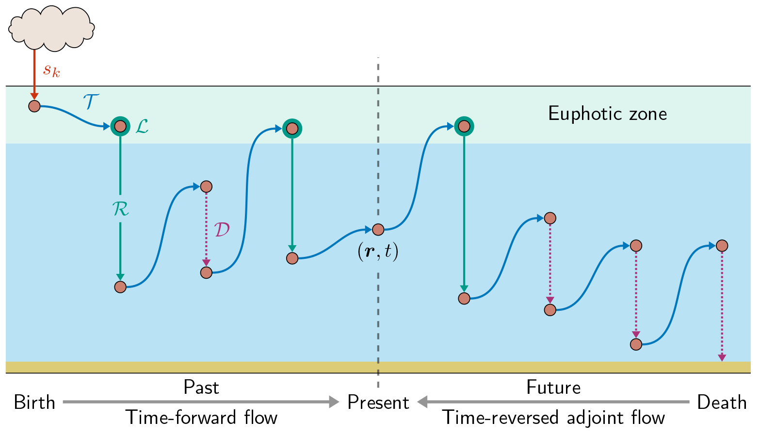
Figure 1Schematic of the birth-to-death life cycle of a labeled DFe molecule (red dot). As captured by Eq. (2), the molecule makes several passages through the biological pump (green, uptake ℒ and regeneration ℛ) and through the scavenging pump (purple dotted, 𝒟) while being transported by the ocean circulation (blue, 𝒯) from its birth (red, sk, here the aeolian source) to its death by eventual burial in sediments following scavenging. This particular DFe molecule passed n = 2 times through the biological pump since its birth and will pass m = 1 times through the biological pump until its death. We consider the DFe concentration at location r and at present time t. Our diagnostics partition DFe at (r,t) into the fractions that have undergone n regenerations since birth and that will undergo m regenerations until death. Computationally, we track DFe from its birth to the present using the usual time-forward flow, while we track DFe backward in time from its death to the present using the time-reversed adjoint flow.
Because the superposition principle applies to the labeling tracers, we can consider the DFe concentrations to be the sum of the concentrations of different iron “source types”: , where χk is the concentration due to source sk. In steady state, we can therefore calculate the concentration χk of each source type by solving (Holzer et al., 2016)
We caution the reader that the equivalent linear model (Eq. 2) is not a linearization of the nonlinear parent model (Eq. 1) in the usual sense. The equivalent linear model is constructed to partition DFe in the unperturbed system. By contrast, linearization usually refers to the first-order Taylor expansion of the nonlinear model around a base state, which captures the system behavior for small perturbations about that base state.
To establish how much a given iron molecule has contributed to organic matter export since its birth, we partition the DFe concentration according to the number of its past passages through the biological pump.
3.1 Iron concentration regenerated n times since birth
We first consider the concentration of DFe that has never been regenerated since it was injected (born) by the source. This concentration, denoted by , can simply be computed from our equivalent linear system by injecting iron labels with source sk, but not permitting them to be regenerated. We therefore remove the ℛ term from Eq. (3), which is equivalent to replacing ℋ with ℱ, to obtain
We use arrow superscripts to indicate past processes that occurred since injection into (↓) the ocean or future processes that will occur until removal out of (↑) the ocean.
We can now calculate the concentration of DFe from source k that has been regenerated exactly one time, , as follows. The source of labels for is the rate of first regeneration of DFe, which is given by . We simply allow the system to cycle these labels but remove them on uptake using ℱ (no second regeneration). Thus, in steady state, obeys . Similarly, the source of DFe that has been regenerated exactly n+1 times since birth is the rate of (n+1)st regeneration. This gives the recursion relation
with Eq. (4) providing the starting point of the recursion. Note that the concentrations partition the DFe concentration exactly, with , as shown in Appendix B.
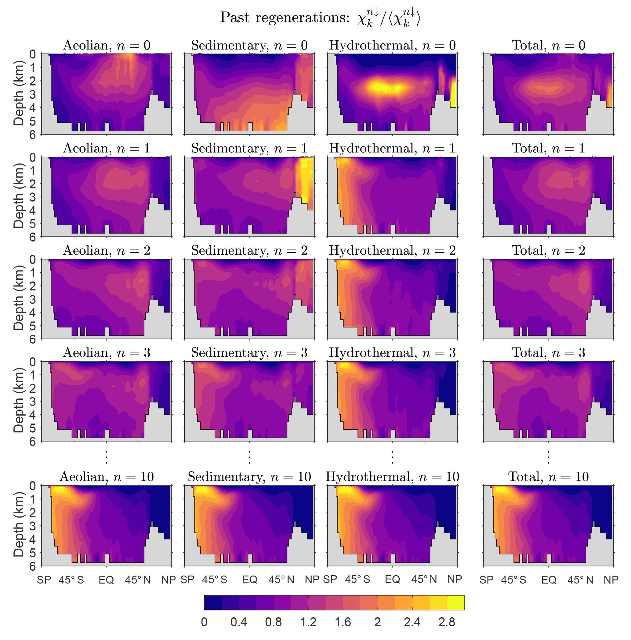
Figure 2Global zonal averages of the concentration of DFe that was regenerated n times since birth, normalized by its global mean, for and 10. The normalized concentrations of the three source types (aeolian, sedimentary, hydrothermal) are shown, as is their sum, which is the total concentration regardless of source type. This figure is for our typical state.
Figure 2 shows global zonal averages of the iron concentration for our typical state, partitioned by source type (aeolian, sedimentary, hydrothermal) and according to the number n of past regenerations since birth. To emphasize the spatial patterns, each field has been normalized by its global volume-weighted average, . Iron that has never been regenerated (n=0) carries a strong source signature, with peak concentrations where the sources are largest. The patterns change dramatically with one passage through the biological pump (n=1). Because iron is regenerated at depth with a Martin power-law profile, the concentration of aeolian DFe that has been regenerated n=1 times has a subsurface maximum at roughly 1500 m of depth. Similarly, sedimentary iron that passed once through the biological pump has a mid-depth maximum and is no longer concentrated near the seafloor. Sedimentary iron that has been regenerated n=1 times is concentrated in the Arctic, presumably because the model has already shallow sedimentary sources there. However, the model's Arctic circulation is poorly constrained (Primeau et al., 2013) and this particular feature may not be robust. Hydrothermal iron that has been regenerated n=1 times shows the signature of Southern Ocean nutrient trapping (Holzer et al., 2014; Primeau et al., 2013) as expected from the fact that hydrothermal iron is injected at seawater densities that outcrop in the Southern Ocean.
As the number n of past regenerations increases, rapidly converges to a pattern that is independent of source type. Physically, this is because the memory of birthplace quickly fades with each passage through the biological pump. Mathematically, this can be seen from recursion Eq. (5), which gives , where . Thus, for sufficiently large n, the concentration becomes proportional to the eigenmode of 𝒜 with the largest eigenvalue λ, and the amplitude of the pattern decays exponentially like , where . (Note that λ<1, as must be the case for to converge to χk.) In other words, as 𝒜 is applied repeatedly, only the projection of onto the eigenmode of 𝒜 with the gravest eigenvalue survives. Because 𝒜 is independent of source type, all source types approach the same large-n asymptotic eigenpattern. Convergence to this pattern is remarkably rapid: for aeolian and sedimentary iron, the pattern has emerged after about five regenerations (not shown) and for hydrothermal iron even sooner. By n=10 the asymptotic pattern is well established and indistinguishable for the different iron source types (bottom plots of Fig. 2).
How robust is the large-n eigenpattern of across our family of solutions? To quantify the approach to the exponentially decaying eigenmode, we plot in Fig. 3a the global mean concentration that has been regenerated n times since birth as a function of n for the five representative state estimates in Table 1. Figure 3a shows that the e-folding scale n* is independent of source type as expected (same large-n slope for all source types on the semilog plots). For all five states the convergence to exponential decay is quickest for hydrothermal iron. The value of the e-folding scale n* depends on the state of the iron cycle. For our five representative states, the smallest n* values occur for the high-source states ( for HiA-LoS and 0.8 for HiH), while the largest e-folding scales occur for the low-source states (1.4 for both HiS-LoA and LoH), with for our typical state. Across the entire family of state estimates, n* ranges from about 0.4 to 2.8. The dependence of n* on source scenario makes sense when we consider that all these states are optimized against the observed DFe concentrations: high aeolian input must be countered by vigorous removal from the surface ocean, and hence a large proportion of the iron in the ocean is accounted for by the first few regenerations since birth, leaving little DFe for multiple regenerations. Conversely, low aeolian input corresponds to less vigorous biological cycling so that a larger portion of the iron is available to pass through the biological pump repeatedly. Similar considerations hold for hydrothermal and sedimentary iron. For all states, asymptotic behavior is well established for n ≳ 5.
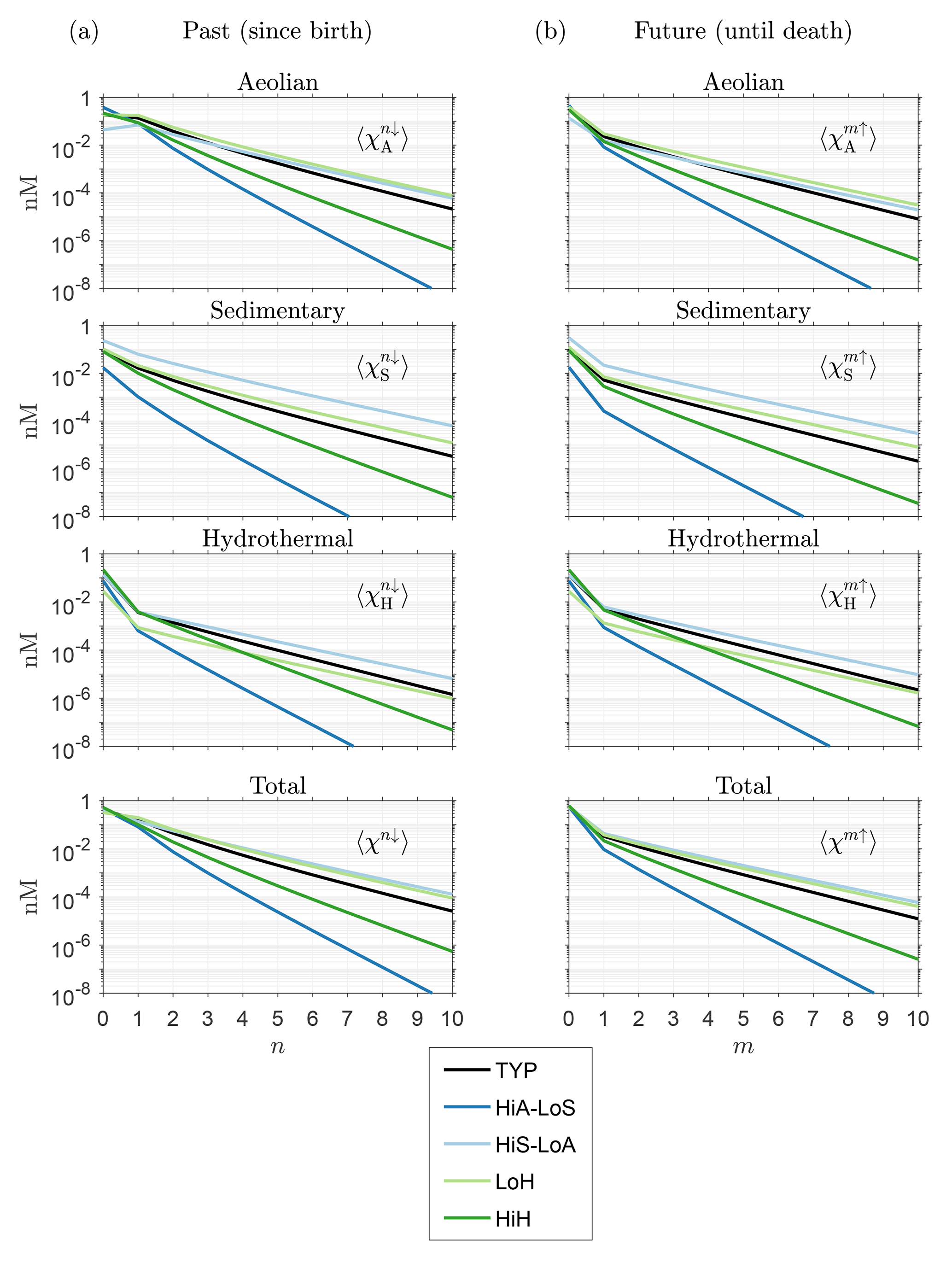
Figure 3(a) Global mean DFe concentration regenerated n times in the past, , as a function of n for five representative states of the iron cycle. (b) Mean concentration regenerated m times in the future, , as a function of m.
The sedimentary and hydrothermal iron concentrations get their largest contributions from iron that has never been regenerated (n=0), again pointing to significant permanent removal of these iron types before they can reach the euphotic zone following injection (birth) at depth. For aeolian iron in the typical, LoH, and HiS-LoA states, the largest contribution comes from iron that has been regenerated n=1 times as all freshly born aeolian iron is immediately available for uptake and regeneration. However, for the high-source states (HiA-LoS and HiH), the largest contribution still comes from iron that was never regenerated because the increased scavenging necessary to balance the high sources prevents most aeolian DFe from being utilized even though it is deposited directly into the euphotic zone.
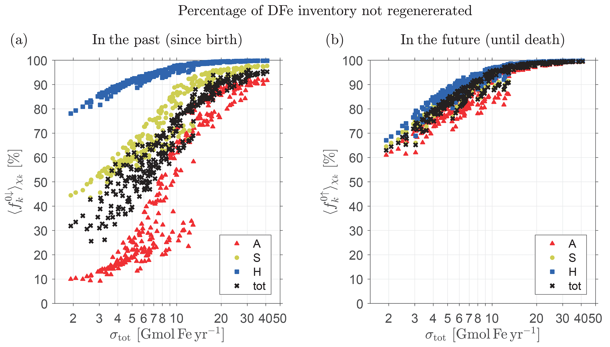
Figure 4(a) Percentage of the total inventory of DFe that has not passed through the biological pump in the past (i.e., since birth) as a function of total source strength, σtot, for the family of state estimates of Pasquier and Holzer (2017). (b) Percentage of the total inventory of DFe that will not pass through the biological pump in the future (i.e., until death). Note the logarithmic abscissa. Shown are the fractional inventories of the individual source types of DFe (color coded) and the total fractional inventory regardless of source type (black).
Figure 3a shows that DFe that has not passed through the biological pump since birth (n=0, unused iron) generally has the highest global mean concentration, except for aeolian DFe under some source scenarios. To quantify the amount of iron that was not regenerated in the past, we now ask how the unused fraction of the global DFe inventory varies with total iron source strength, σtot. Note that this fraction can be considered to be the χk-weighted global average of the local unused fraction . This weighted average is defined as , where we introduced the notation, which will be used throughout. The unused fractional DFe inventory regardless of source type is given by 〈f0↓〉χ, where .
Figure 4a shows the fractional unused DFe inventories and 〈f0↓〉χ as a function of σtot for every member of our family of state estimates. We emphasize that Fig. 4 does not show the response of the iron cycle to changes in σtot, but instead shows the fraction of the unused DFe inventory for distinct equilibrium states, each of which was optimized against observations under a different prescribed iron source scenario (Pasquier and Holzer, 2017). Because the total iron inventory is well constrained across the family, the bulk iron lifetime τ, given by the ratio of inventory to source (see also Table 1), is inversely proportional to σtot, and hence the mean iron age also scales with (σtot)−1 (Holzer et al., 2016). The systematic increase in the fractional inventory of unused iron, and its approach to saturation at 100 % for the largest sources seen in Fig. 4a, reflects the fact that the probability of past regeneration decreases with the mean iron age until the age becomes so short that very little iron has a chance to pass through the biological pump before having to be scavenged out of the system to match the observed DFe concentrations and inventory. For our smallest total source of σtot∼2 Gmol Fe yr−1, DFe molecules have lived long enough to be regenerated at least once with %, while for our largest total source of σtot∼40 Gmol Fe yr−1, most DFe molecules have not had sufficient time to be regenerated and %. For state estimates with σtot>7 Gmol Fe yr−1, more than half of the DFe in the ocean has never passed through the biological pump, i.e., %.
Figure 4a also shows that the fraction varies significantly with iron source type k. This is because the probability of a past passage through the biological pump is strongly dependent on birth location. The fraction that has not been regenerated since birth is lower for aeolian DFe than for benthic DFe. Benthic DFe must first be transported to the euphotic zone to participate in biological production and is therefore more likely to be scavenged en route compared to aeolian DFe, which is directly injected into the surface. Hydrothermal DFe is the least likely to have passed through the biological pump, with % for all states and % for states with σtot>7 Gmol Fe yr−1. For sedimentary DFe, % for all states, and % for states with σtot>7 Gmol Fe yr−1. As the mean age becomes ever smaller with increasing σtot, the unused fractional benthic DFe inventory saturates faster to 100 % than the unused fractional aeolian DFe inventory, which reaches only ∼90 % even for σtot∼40 Gmol Fe yr−1, again reflecting greater probability of biological utilization for surface-injected iron. We will return to Fig. 4b below when we explore future passages through the biological pump.
To explore the variations of the asymptotic eigenmode pattern across our different state estimates, Fig. 5 shows the zonally averaged patterns of for n=10, which is well within the asymptotic regime, for our five representative states. (Recall that individual source types all converge to the same pattern, which is hence also the pattern of the total iron concentration.) While there is a signature of Southern Ocean nutrient trapping for all states, there is also significant variation across the state estimates. Broadly, the Southern Ocean trapping has a stronger influence on the eigenmodes of ℱ−1ℛ for the high-source states than for the low-source states. This is likely due to the fact that high-source states are able to match the observed DFe concentrations by having both more active biological iron pumps and scavenging. The transport to depth by both the biological pump and by scavenging particles (the “scavenging pump”) enhances the Southern Ocean trapping. The scavenging is largest at tropical and high latitudes so that stronger scavenging will tend to remove iron from low and high latitudes (see Appendix C for zonally averaged death rates). At high latitudes this is counteracted by stronger trapping, but at low latitudes the death rate dominates and the concentration of iron that passes many times through the biological pump is strongly diminished. Conversely, for the low-source states, reduced scavenging allows iron to pass many times through the biological pump without being scavenged out of the system at low latitudes. Consequently, the low-source states have iron that has been regenerated many times flowing out of the Southern Ocean with mode and intermediate waters well into the Northern Hemisphere.

Figure 5Normalized global zonal averages of the concentration of DFe that has passed n = 10 times through the biological pump since birth regardless of source type, χ10↓, to show the eigenpatterns of our five representative state estimates (Table 1). The zonal averages are normalized by the global mean.
3.2 Mean number of regenerations since birth
A key metric of how much the DFe field has contributed in the past to organic matter export is the mean number of times, , that a given iron molecule has been regenerated since its birth. From the local fraction of the total DFe that was regenerated n times since birth, , the mean number of past regenerations is by definition given by . Mathematically, as shown in Appendix B, it follows from Eq. (5) that obeys
Physically, Eq. (6) may be interpreted as the equation for a labeling tracer that is cycled just like DFe by the ℋ operator, but whose numerical value accumulates -fold with past regenerations. Computationally, solving Eq. (6) provides an efficient means of finding that avoids first finding and explicitly summing .
A given iron molecule at r is responsible, on average, for the export of iron molecules of source type k since its birth. The corresponding organic matter export is quantified by the mean number of phosphorus molecules that are exported along with the iron. The regeneration operator for phosphorus is given by , where is diagnosed from the optimized phosphorus uptake of the underlying model (Pasquier and Holzer, 2017). The mean number of phosphorus molecules, , globally exported and remineralized in the past per DFe molecule that is currently at r obeys
In other words, on average, one of the type-k DFe molecules currently at r has supported the export of phosphorus molecules since its birth. In analogy with Eq. (6), we interpret Eq. (7) as defining a labeling tracer that is cycled like DFe by the ℋ operator, but whose numerical value counts the number of phosphate molecules that were regenerated in the past via the phosphate regeneration operator ℛP.
Figure 6 shows the global zonal averages of for our typical state estimate. Note that the maximum values of are order unity and, on average, most of the iron in the ocean has been regenerated less than once since its birth. Iron with the largest is found near the Southern Ocean surface and in mode and intermediate waters flowing out of the Southern Ocean, which is presumably a signature of Southern Ocean nutrient trapping. In terms of source types, aeolian iron has been most active in the biological pump with exceeding 0.6 throughout most of the ocean interior and exceeding 1.0 throughout much of the Southern Ocean water column. In the surface waters of the low-production subtropical gyres approaches zero. The mean number of regenerations since birth is much smaller for sedimentary and hydrothermal iron, again reflecting the greater scavenging hazard for benthic iron. For sedimentary and hydrothermal iron, values of greater than 0.5 extend from the subantarctic Southern Ocean surface into mode and intermediate waters where scavenging is relatively weak (Appendix C).
The zonally averaged patterns of are remarkably similar across our family of estimates. As shown in Appendix D, the spatial patterns are also insensitive to the value of the recyclable fraction of scavenged iron, frec, although their amplitude can vary by a factor of ∼2 between the frec=0 and frec=1 extremes. The patterns of the global zonal averages of (not shown) are nearly identical to those of .
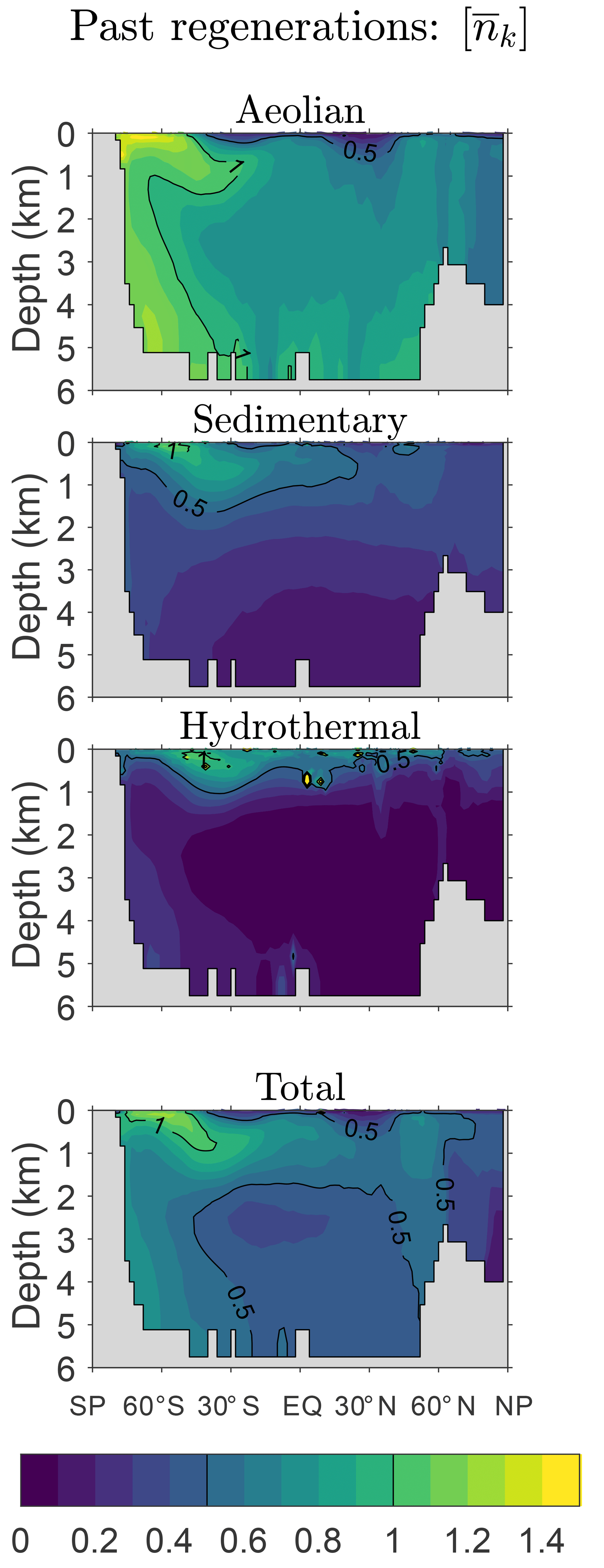
Figure 6Zonal averages of the mean number of past passages through the biological pump (i.e., since birth), . This figure is for our typical state.
We expect significant variations in the amplitudes of and (the mean number regardless of source type) across the family of state estimates. Because the number of regenerations that are possible during the lifetime of an iron molecule should be proportional to the bulk iron lifetime , we expect . To test this and to quantify the range of possible variations, Fig. 7a shows the global average as a function of σtot on a log–log plot and Fig. 7b shows the corresponding behavior for . Both and exhibit the expected approximate inverse relation with σtot. Note that the scaling is not exact; instead, Fig. 7a suggests that there are scaling regimes for a low-source cluster and for a high-source cluster, with a transition for intermediate source strengths. This approximate nature of the scaling reflects the fact that the timescale for a passage through the biological pump is not merely set by the prescribed circulation and (in our model) instant particle transport and remineralization, but also depends on the spatial distribution of the scavenging, which varies with the optimized source scenarios. The detailed timescales that link circulation, scavenging, and pumping frequency will be explored in a future publication. The numerical values of range from 0.05 for σtot=41 Gmol yr−1 to 2.2 for σtot=1.9 Gmol yr−1, while correspondingly ranges from approximately 0.4 to 4.3 mol P (mmol Fe)−1 (i.e., from 40 to 460 mol C (mmol Fe)−1 using a simple uniform Redfield C : P ratio of 106:1 for unit conversion).
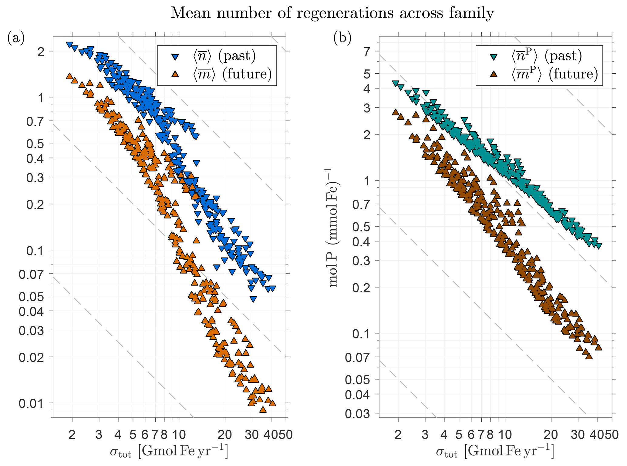
Figure 7(a) The globally averaged mean number of past and future DFe passages through the biological pump per injected DFe molecule (regardless of source type), and , as a function of the total iron source strength, σtot, for the family of state estimates of Pasquier and Holzer (2017). (b) The corresponding globally averaged mean number of phosphorus molecules exported per DFe molecule, and . Note the log–log axes to highlight the approximate inverse relationship with σtot. To guide the eye, dashed grey lines indicate an exact power law.
We now ask how many times a given DFe molecule in the ocean will get regenerated in the future before eventually being permanently scavenged out of the system. The natural way to formulate the necessary equations is to consider the time-reversed adjoint flow (Holzer and Hall, 2000), for which the system is governed by the adjoint operators , , , and . These adjoints are defined in terms of the volume-weighted inner product , where the integral ranges over the entire ocean volume. Thus, , the adjoint of ℋ, is defined as usual so that . In the time-reversed adjoint flow, the death operator becomes a source of labels that we then track through sequential regenerations backward in time to the present, analogously to what we did in the previous section for the usual time-forward flow. The use of adjoint operators allows for numerically efficient evaluation of our diagnostics because a single tracer injected at death into the time-reversed adjoint flow suffices to produce the full three-dimensional concentration fields of interest at present. Here we provide the key equations – their derivation in terms of Green functions is detailed in Appendix E.
4.1 Number of regenerations until death
To compute the number of future regenerations, it is useful to calculate the death rate d(r) with which iron is permanently (nonreversibly) removed at point r. This death rate can be diagnosed from the scavenging operator 𝒟 and the DFe concentration χ(r) as detailed in Appendix C, where we also show basin zonal averages of d(r). The corresponding rate constant γ𝒟 for the linear equivalent model is defined such that d(r)=γ𝒟(r)χ(r).
One can show that the local fraction f↑(r) that eventually dies obeys
where uniformly everywhere because all DFe must eventually be scavenged out of the system.
In analogy with Eq. (4), the fraction f0↑ that is regenerated zero times until death obeys
By using the regeneration rate of DFe that will be regenerated m times until death and going back in time by one regeneration, we obtain the fraction that will be regenerated (m+1) times until death, giving us the recursion relation
Note that as can be verified from Eq. (9) and Eq. (10).
The mean number of regenerations until death, , can be shown to obey
The mean number of phosphorus molecules, , globally exported and remineralized in the future per DFe molecule that is currently at r obeys
In other words, on average, a DFe molecule currently at r will support the export of phosphorus molecules before it is buried in the sediments.
Figure 8 shows the zonally averaged fraction fm↑ of DFe that will undergo m regenerations in the future normalized by the global average, 〈fm↑〉, to emphasize changes in the pattern with m. Note that this fraction is the same for all source types because the future of a given DFe molecule is independent of its past. Below the thermocline, the pattern of f0↑ is nearly uniform at a value just above its global mean but drops to below 50 % of the global mean near the surface where the probability of further biological utilization and regeneration is largest (careful inspection is required to see this in Fig. 8). The pattern of f1↑ has its largest amplitude at the surface and in the Southern Hemisphere, where it spreads deepest from the surface, reflecting the relatively low Southern Hemisphere death rates (Appendix C). As m increases, fm↑ becomes rapidly proportional to the gravest eigenmode of (see Eq. 10). As this eigenmode is approached, the pattern of fm↑ contracts into the Southern Ocean, presumably because iron that will be regenerated many times before death can only be found where there is both a low death rate and efficient nutrient trapping.
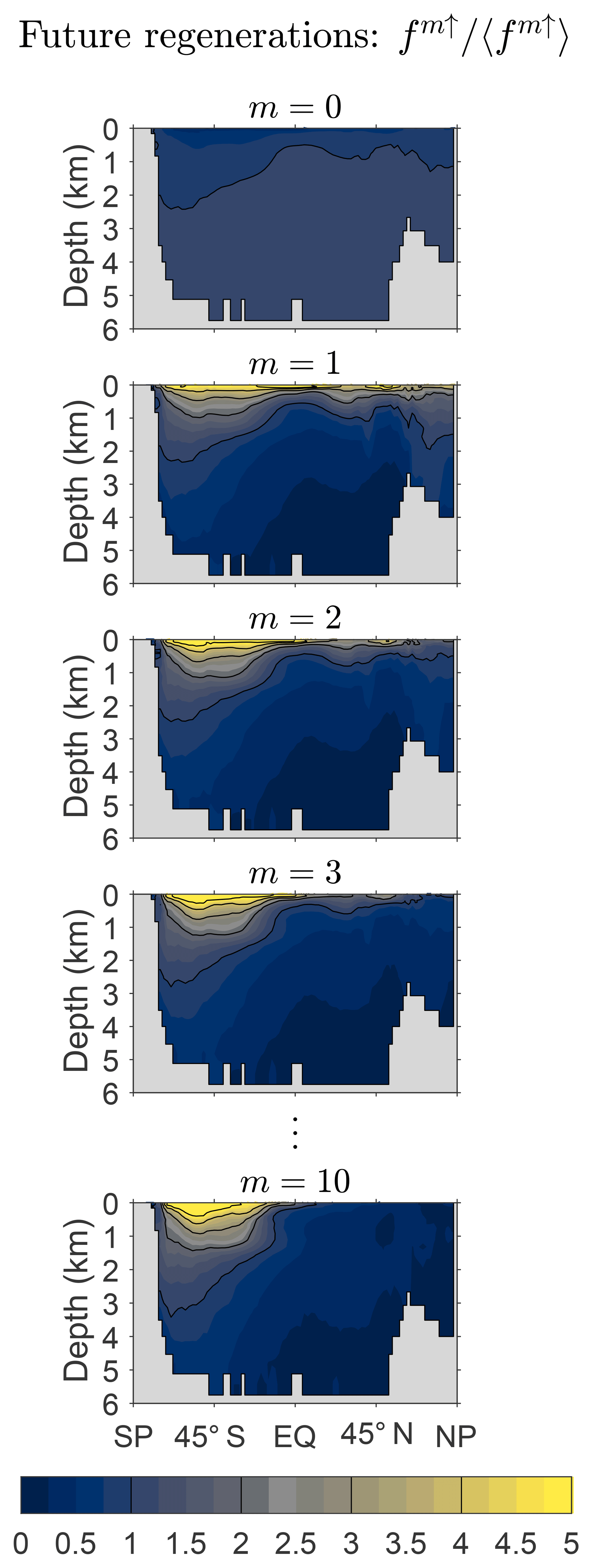
Figure 8Global zonal averages of the fraction of DFe that will be regenerated m times, fm↑, normalized by its global mean value, 〈fm↑〉, for and 10. This figure is for our typical state.
To quantify the approach of fm↑ to the gravest eigenmode of , we return to Fig. 3b, which shows the global averages of the corresponding DFe concentrations as a function of m. Note that and ℱ−1ℛ have the same eigenvalues so that and approach the same exponential decay (Fig. 3a and b).
We return to Fig. 4b to consider the fractional DFe inventories that will not pass through the biological pump in the future for all our state estimates. These inventories for source type k and regardless of source type are given by and 〈f0↑〉χ. We expect the probability of future regenerations to increase with the remaining lifetime of DFe, which should also scale like given a well-constrained global DFe inventory. This is confirmed in Fig. 4b by the systematic increase and approach to 100 % saturation of and 〈f0↑〉χ with increasing σtot. (Note that in the theoretical σtot→0 limit, we expect and , although our lowest sources are not nearly small enough to exhibit this limiting behavior.)
Figure 4 shows striking asymmetries between unused past and future inventories. The fractional inventory of iron that will not be utilized in the future (Fig. 4b) is nearly independent of iron type k, in sharp contrast with the fractional inventory that was not utilized in the past (Fig. 4a). The insensitivity of to source type is due to the independence of f0↑ on source type so that the χk-weighted global average is only sensitive to changes in the pattern of χk, which varies little across the family of states (Pasquier and Holzer, 2017). Note that for a given σtot, the inventory of total DFe unused in the future, 〈f0↑〉χ, is significantly larger than the inventory of total DFe unused in the past, 〈f0↓〉χ. In other words, total DFe is more likely to have been regenerated in the past than it is to be regenerated in the future. This asymmetry stems from the fact that is dominated by the relatively small unused aeolian fraction (see Fig. 4a). In terms of individual source types, aeolian and sedimentary DFe are also more likely to have been regenerated in the past than in the future, but the reverse is true for hydrothermal DFe for which the scavenging hazard following birth is greatest. Thus, for a hypothetical state in which hydrothermal iron dominates the total DFe inventory, it is possible that one could get ; however, none of our states fits this scenario.
We now return to the asymptotic eigenpatterns of fm↑. How robust are these eigenpatterns across our family of state estimates? Figure 9 shows f10↑ normalized by its global mean and zonally averaged over the global ocean for our five representative states (for m=10, fm↑ is an excellent approximation to the gravest eigenmode of ). While there is some variation across the family, the patterns are qualitatively similar. Because the natural quantity that keeps track of future regenerations is the source-type-independent fraction of DFe that will undergo m regenerations, the spread in the large-m pattern of fm↑ across the family of states is much smaller than the spread in the large-n pattern of ( being the natural quantity for keeping track of past regenerations).
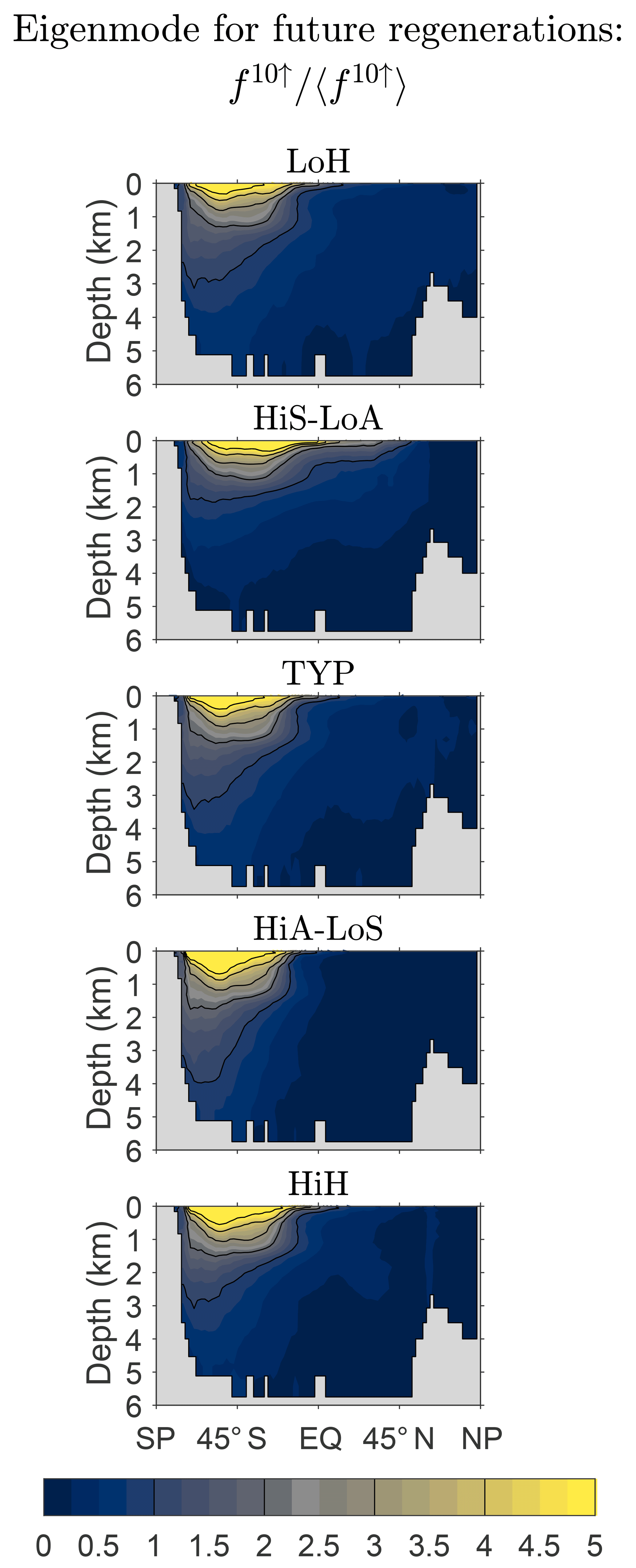
Figure 9Global zonal averages of f10↑ normalized by their global means, 〈f10↑〉, to show the approximate asymptotic eigenpatterns for five representative state estimates.
Figure 10a shows the global zonal average of the mean number of future regenerations , which like fm↑ is independent of source type. The pattern of is similar to the pattern of f1↑, which dominates the rapidly converging sum . The pattern is surface intensified and largest in the Southern Ocean. decays rapidly with depth, reflecting the fact that the deeper the DFe, the harder it will be to escape death on the way to the surface to participate in the biological pump. These qualitative features are robust across the family of state estimates (not shown). Figure 10b shows that the pattern of the global zonal average of is almost indistinguishable from that of . This is because the patterns of and are dominated by the phosphorus and iron export productions, respectively, which are similar despite the substantial spatial variations of the Fe : P uptake ratio (Pasquier and Holzer, 2017).
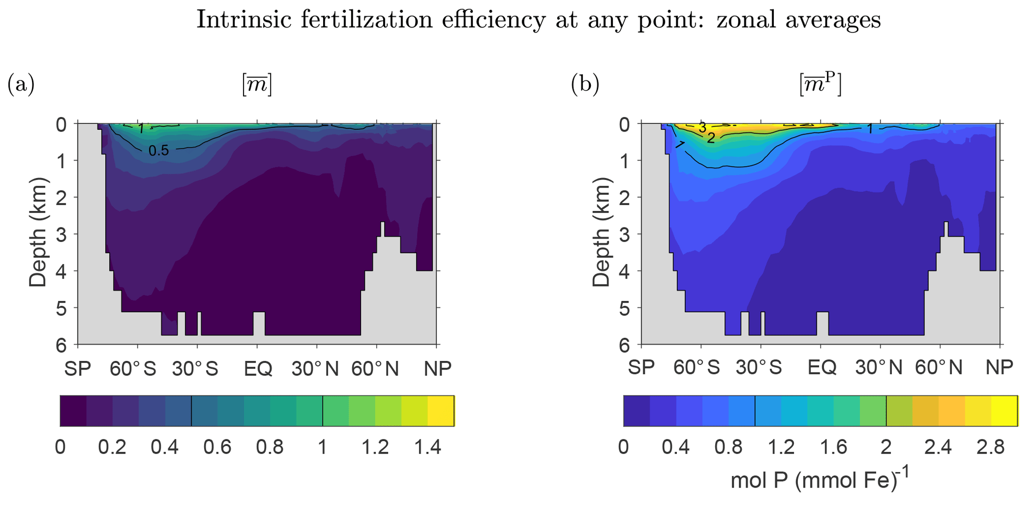
Figure 10Three-dimensional intrinsic fertilization efficiency metrics for our typical state, zonally averaged across the global oceans. (a) The mean number of iron molecules, , that will be regenerated per iron molecule at r during that molecule's lifetime. (b) The corresponding mean number of phosphorus molecules, , that will be regenerated.
Returning to Fig. 7b, we see that both and are again approximately proportional to , as expected. The magnitude of remains at or below order unity and ranges from 0.01 to 1.4 as σtot varies from 41 to 1.9 Gmol yr−1. Correspondingly, ranges from 0.07 to 2.8 mol P (mmol Fe)−1 or from 7 to 290 mol C (mmol Fe)−1 when converted using C : P .
5.1 Export supported per unit DFe injection at r
We begin by asking how much an arbitrary (“test”) source sk(r) contributes to the globally integrated export and remineralization of iron and phosphate in organic matter. (In our model all exported phosphorus is instantly respired with the divergence of a Martin POP flux profile – DOP is not explicitly modeled.) We first consider the global export that will be supported per unit injection of DFe at point r. The concentration response to a unit injection is the Green function associated with operator ℋ, and the global export due to this response is simply obtained as the global integral of the regeneration operator ℛ acting on this response. As shown in Appendix F, a DFe injection into volume element d3r at rate sk(r)d3r supports a globally integrated iron export rate, Φk(r), given by
while the corresponding phosphorus export, , is given by
These equations have a straightforward physical interpretation: the mean number of future regenerations, , is simply the number of DFe molecules that will be exported per DFe molecule injected at point r, and is the corresponding number of phosphorus molecules that will be exported. The quantities and are hence measures of the efficiency of iron fertilization at point r. Note that this local efficiency is independent of source type; the efficiency is determined by the biological pump and the transport of water, neither of which depend on the iron source type. Furthermore, the local efficiency is defined regardless of whether an iron source is actually present at r. The efficiency quantifies the global phosphorus export rate per unit DFe source rate at r. At all points r, even where there is no actual source in the system, can be considered to be the “sensitivity” of the linear equivalent system to the insertion of the arbitrary test source sk(r): Eq. (14) shows that is the proportionality between the export response and the test source sk(r). In this sense, the fertilization efficiency is a close, but distinct, cousin of the sensitivity to small-amplitude perturbations considered by Dutkiewicz et al. (2006).
Viewed another way, by construction and are the mean numbers of DFe and phosphorus molecules exported per molecule of iron that is present at r in the current state of the ocean, before that molecule is buried. Thus, and again have the natural interpretation of being fertilization efficiencies. We emphasize that and are defined without perturbing the system and are hence noninvasive metrics of what we call the intrinsic iron fertilization efficiency. The plots of the zonally averaged and in Fig. 10 may thus be interpreted as zonal averages of this intrinsic, three-dimensional iron fertilization efficiency, which can be seen to be highest at the surface and rapidly diminishes with depth. The zonal averages of and are dominated by the Southern Ocean. However, we will see that the Southern Ocean only plays a secondary role for the fertilization efficiency at the surface.
Figure 11a shows that the surface patterns of are qualitatively similar across the five representative states, with a broad maximum in the central tropical Pacific and secondary maxima in the subpolar oceans. The states with the largest global mean surface fertilization efficiency, , (values provided in Fig. 11a) are the low-source states as one would expect: the less iron is in the system, the more the biological pump is expected to benefit from the iron present. For the HiS-LoA state, a typical molecule of DFe at the surface leads to a globally integrated export of molecules of iron. For the high-source states (HiA-LoS and HiH), both the tropical Pacific and the Southern Ocean are locally most prominent, but the surface mean efficiencies are only (HiA-LoS) and 0.5 (HiH) molecules of iron exported per typical surface molecule.
Figure 11b shows the surface patterns of the efficiency for fertilizing organic matter export, . The global surface average, , is again highest for the low-source states. However, varies less across our representative states than (a range of ∼3 compared to ∼7). This is consistent with the fact that all states have very similar phosphorus exports (well constrained by the data used in the optimizations), but widely differing iron exports and Fe : P uptake ratios (Pasquier and Holzer, 2017).
The surface patterns of and are similar, with very similar systematic variations across the different states. However, because of the iron dependence of the Fe : P uptake ratio, has sharper gradients than , with a more pronounced contrast between the low-efficiency subtropical gyres and the high-efficiency tropical Pacific. The Fe : P uptake ratio in our model is proportional to , which has its lowest values of around 0.1 in the central and eastern tropical Pacific for all our states. The corresponding P : Fe uptake ratio (not shown) has a global pattern that is broadly similar to the pattern of the intrinsic fertilization efficiency because large P : Fe means that a relatively large number of P molecules are taken up (and hence exported) per utilized DFe molecule. The correspondence is not exact, but the P : Fe uptake ratio plays a central role in shaping at the surface. At depth, the effect of the P : Fe ratio on is less important because, depending on where the DFe reemerges into the euphotic zone, deep DFe will not necessarily be utilized in regions of high P : Fe.
The key result of Fig. 11 is that regardless of state, the tropical Pacific is where iron has its highest intrinsic fertilization efficiency. For high-source states, the fertilization efficiency of the Southern Ocean can be equally as large, although the global surface mean efficiency is much lower than for low-source states. The efficiency is not highest in the eastern tropical Pacific where production is highest because of the associated large scavenging rate due to organic particles. The sweet spot between upwelling-fertilized production and relatively low scavenging lies in the central tropical Pacific to the west of the highest productivity. The state-dependent relative importance of the Southern Ocean compared to the tropical Pacific is a complicated function of how our optimized states match the nutrient observations and reflects a delicate balance between fertilizing biological production and the resulting enhanced scavenging. Interestingly, Dutkiewicz et al. (2006) found that the sensitivity of their coupled model to aeolian iron addition is also largest in the central tropical and eastern Pacific. This suggests that the intrinsic fertilization efficiency of the unperturbed state is shaped by similar processes as the sensitivity to small-amplitude perturbations.
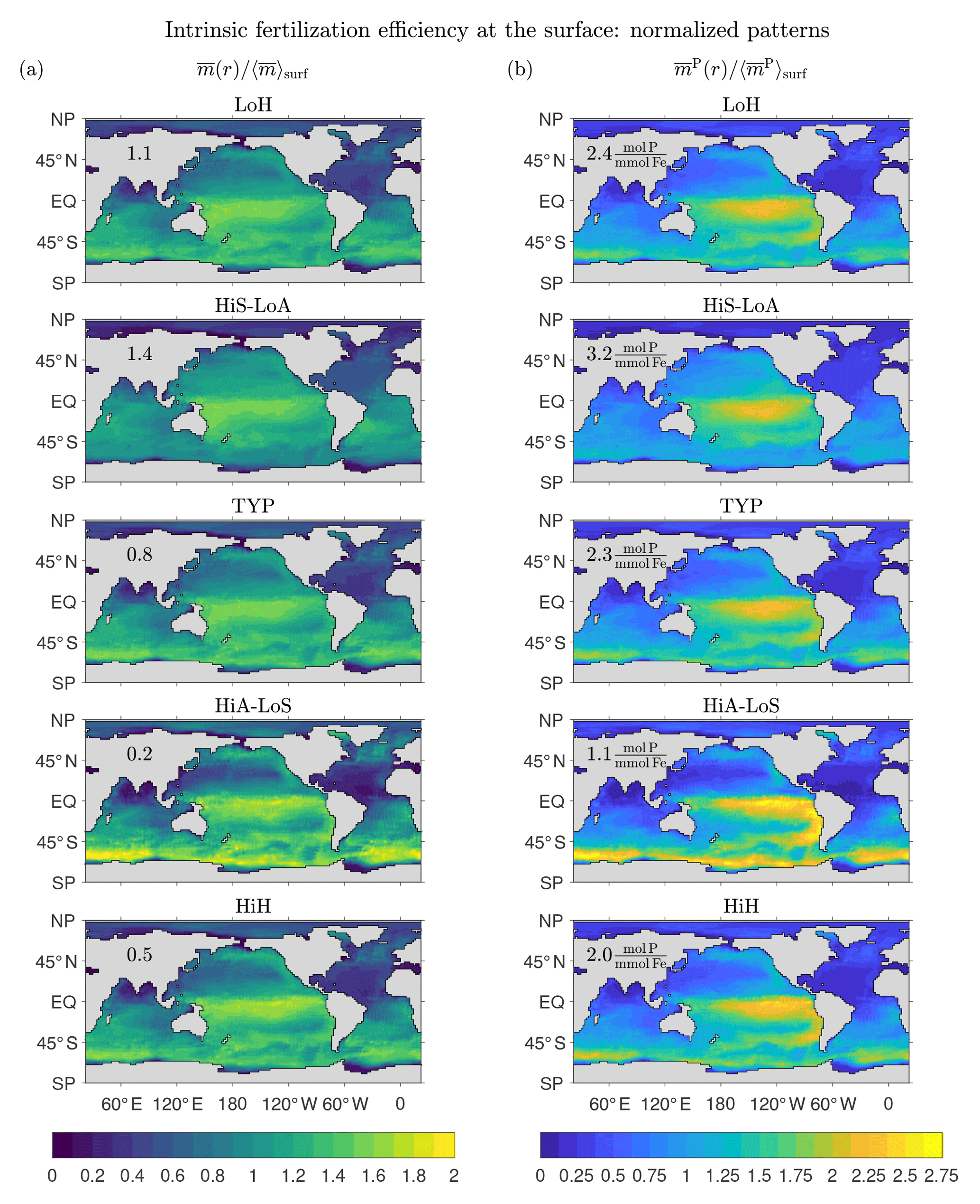
Figure 11Normalized patterns of our intrinsic fertilization efficiency metrics at the surface. (a) The mean number of iron molecules, , that will be regenerated per iron molecule at surface point r during that molecule's lifetime. (b) The corresponding mean number of phosphorus molecules, , that will be regenerated. To allow for a meaningful comparison of the patterns of different states, and have been normalized by their global surface averages, and (values are given in each plot).
How do our estimates of intrinsic fertilization efficiency compare to previous estimates of differently defined fertilization efficiencies? Across our entire family of estimates, has a range of 0.7–7 mol P (mmol Fe)−1, which converts to 73–750 mol C (mmol Fe)−1 using a simple uniform C : P ratio of 106:1. Thus, our estimate of the intrinsic fertilization efficiency is roughly 1 to 2 orders of magnitude larger than the estimate of about 3.3 mol C (mmol Fe)−1 by Zeebe and Archer (2005), who reported 900 t C exported for 1.26 t of iron added during the SOFeX artificial fertilization experiment. There are multiple reasons why our estimate of fertilization efficiency differs from that of Zeebe and Archer (2005). First, the latter is a regional estimate based on a localized artificial fertilization experiment, while the former is a global mean estimate of the unperturbed system. Second, Zeebe and Archer (2005) used the data from the iron fertilization experiments without any corrections for ligand protection in the natural unperturbed system, which leads to an underestimate of the natural fertilization efficiency. de Baar et al. (2008) correct for this in their analysis, giving an estimate of 2.6–100 mol C (mmol Fe)−1 for the natural fertilization efficiency. Despite being inferred from a finite-amplitude perturbation experiment, the estimate of de Baar et al. (2008) overlaps with the low end of our estimates (which corresponds to the possibly more realistic high-source states). The sensitivity of global production to perturbations in the local aeolian source estimated by Dutkiewicz et al. (2006) has a spatial distribution with a range of about 20–180 for a 0.02 perturbation. The model of Dutkiewicz et al. (2006) exports one-third of its production as POP so that these sensitivities translate to a POP export per added DFe molecule of about 28–250 mol C (mmol Fe)−1, a lower bound on the full carbon export and about a third of the intrinsic fertilization efficiency estimated here. We emphasize that differences between these various estimates are not only due to uncertainties in the iron cycle (as expressed by our range of values), but also due to differences in the definition of fertilization efficiency, not to mention due to differences among models and methodologies.
5.2 Relation to relative export efficiency
To compare the importance of the different iron source types in the current state of the ocean, Pasquier and Holzer (2017) defined the export-support efficiency of iron type k as , where is the fraction of the global phosphorus export supported by source type k and is the fractional global source of type k. We found that a key metric that is robust across our family of state estimates is the relative export-support efficiency, , which is the ratio of the export-support efficiency of source type k to the export-support efficiency of the other source types, whose combined source is the complement .
It follows algebraically from Eq. (14) that the relative export efficiency can be expressed as
where is the sk-weighted global mean, defined so that for any field x(r), and is the corresponding -weighted global mean. Thus, the relative export-support efficiency is the ratio of the mean intrinsic fertilization efficiency of the source to the mean intrinsic fertilization efficiency of its complement.
Pasquier and Holzer (2017) found that all members of the family of state estimates share approximately the same relative export efficiencies of , , and , where the uncertainties represent the scatter across the family. What is new here is Eq. (15), which relates the global metric to source-weighted averages of the local intrinsic fertilization efficiency, .
Our analysis comes with a number of caveats that should be kept in mind. Some of these were already identified in the work of Pasquier and Holzer (2017), in which the design of our coupled Fe–P–Si inverse model is presented in detail. In particular, the model used DFe data from the GEOTRACES Intermediate Data Product (IDP) 2014 (in addition to an older compilation by Tagliabue et al., 2012), which did not contain the newer data from the Pacific and Southern Ocean made available only recently in the GEOTRACES IDP 2017. Although it is inevitable that assimilating the additional constraints of the IDP 2017 would lead to some quantitative changes, especially in the Pacific, we think that including the IDP 2017 data would not lead to qualitative changes. The states used here do feature strong Pacific DFe plumes of about the observed spatial extent to the west of the East Pacific Rise (EPR), but unlike the observations these plumes also extend to the east of the EPR. The unrealistic eastward plume would not be corrected by assimilating the IDP 2017 data into the biogeochemical model because it is due to small biases in the underlying circulation, which we hold fixed throughout. The deep Pacific circulation can be corrected by assimilating δ3He into a circulation inverse model, but this is beyond the scope of the current study. Moreover, any quantitative differences due to additional constraints would very likely be much smaller than the variations across our family of state estimates, given its 2-order-of-magnitude range in iron source strengths.
While the state estimates used were optimized against the observations available at the time, we note that the sedimentary sources of the underlying inverse model of Pasquier and Holzer (2017) are keyed to the flux of particulate organic matter into the bottom box where the organic matter is completely oxidized in our model of the phosphorus cycle. This parameterization of the sedimentary source is based on observations along the California coast of a correlation between the DFe flux from sediments and the flux of oxidized organic matter (Elrod et al., 2004). All the model's sediment sources are thus reductive as is the case in many current iron models (Aumont and Bopp, 2006; Moore and Braucher, 2008). However, the analysis of δ56Fe by Conway and John (2014) has highlighted the importance of non-reductive sources, which our inverse model does not include. Our state estimates feature sedimentary sources that are realistically dominated by the continental shelves (Pasquier and Holzer, 2017), but they also include sources that are 1 to 2 orders of magnitude smaller below highly productive regions in the eastern tropical Pacific, where a sluggish abyssal circulation allows some DFe to accumulate at depth, as can be seen in Fig. 2. Similarly, our hydrothermal sources inject DFe into the ocean where it is then protected from rapid scavenging by our enhanced ligand concentrations near hydrothermal vents. However, the recent work of Fitzsimmons et al. (2017) suggests that this model of hydrothermal iron needs to be revised in the future to include reversible exchange between DFe and particulate iron, which is currently omitted in our scavenging parameterization. Regarding ligands, the inverse model of Pasquier and Holzer (2017) prescribes an optimized distribution of a single type of ligand that is enhanced in hydrothermal plumes and in old waters, with optimized parameters. Ligands are not dynamically transported and the effect of different ligand types on iron bioavailability (Maldonado et al., 2005) is neglected.
Other caveats relate to biogeochemical parameters that could not be optimized. The recyclable fraction, frec, of DFe scavenged by opal and POP was prescribed to be 90 % for all scavenging particles. frec is highly uncertain and in recent models its value has spanned the entire 0–100 % range (Frants et al., 2016; Galbraith et al., 2010; Moore and Braucher, 2008). We established the sensitivity of our results to the value of frec by generating new state estimates from our typical state by prescribing different values of frec ranging from 0 to 100 % and re-optimizing the scavenging and source parameters following the strategy of Pasquier and Holzer (2017) (see Appendix D for details). We find that the patterns of and are robust to changes in frec, although their global mean values, which are order unity for the re-optimized typical state with frec=0, systematically decrease by roughly a factor of 2 when frec is increased to 100 %. The mean numbers of past and future phosphorus molecules exported per DFe molecule, and , are robust to changes in frec in both pattern and magnitude. This robustness reflects the fact that the optimization can compensate for changes in the scavenging pump with changes in the biological iron pump.
A key control on our model results is the Fe : P stoichiometry. The model approximates the iron dependence of the Fe : P uptake ratio by a Monod function with a half saturation constant that is the same for all phytoplankton classes. We acknowledge that this may not be realistic. For example, Kirchman (1996) suggested that including the microbial “ferrous wheel”, which operates with different stoichiometric ratios, could affect iron budgets in the euphotic zone. Similarly, Strzepek et al. (2005) explored variations in the iron regeneration rates of different organisms and cautioned modelers to pay careful attention to the details of the Fe:C stoichiometry. Relatedly, our model simply remineralizes iron in the same Fe : P ratio with which it was utilized so that the vertical profiles of iron and phosphate remineralization have identical shapes. However, measurements by Twining et al. (2014) show that, at least for some phytoplankton species, iron is remineralized more slowly than phosphate, suggesting that our remineralization profile for iron could be too shallow. Different remineralization length scales for iron and phosphate were also emphasized by Boyd et al. (2017). Because our model is optimized to fit the DFe observations with an emphasis on deep profiles relative to surface measurements (Pasquier and Holzer, 2017), a potentially too-shallow remineralization of iron would be compensated for by an increased strength of the biological pump. Furthermore, the relative amount of scavenging by opal and POP particles is optimizable in our model so that deeper iron remineralization can be achieved by increasing the scavenging by opal. We acknowledge, however, that when optimizing the match to observed DFe, the model may produce biases in the relative contributions of the biological and scavenging pumps, which would affect our estimates of the number of passages through the biological pump.
The recent work of Rafter et al. (2017) suggests that in surface waters DFe must be preferentially recycled compared to nitrate in order to sustain the observed nitrate consumption in the iron-limited equatorial Pacific. While we do not model the nitrogen cycle, it is reasonable to assume that in the euphotic zone DFe may also be preferentially recycled compared to phosphate. At face value, this appears to contradict our assumption that the detrital fractions, fc, are identical for Fe, P, and Si export. However, the uptake and export of DFe in our model are proportional to the product fc RFe : P, and RFe : P is optimized so that any difference between the iron and phosphate detrital fractions is simply absorbed into RFe : P. However, this does point to the need for caution when interpreting the optimized values of RFe : P.
Importantly, we would like to note that not every process thought to influence DFe needs to be explicitly modeled for a useful representation of the iron cycle. The model of Pasquier and Holzer (2017) is of intermediate complexity, and effects due to processes not explicitly modeled are captured implicitly when parameters are optimized to fit the observed nutrient and phytoplankton fields. Explicit modeling of all known processes in their full complexity may be important for models that try to predict how the system will change in the future, but this is neither necessary nor desirable for constraining and diagnosing the large-scale cycling of DFe in the current state of the ocean as we do here.
We have presented a new conceptual and mathematical framework for quantifying the contribution of DFe to the biological pump during its journey from birth by an external source to death by irreversible scavenging and burial. New diagnostics were developed to partition the DFe concentration into the fraction that was regenerated n times in the past or that will be regenerated m times in the future. These diagnostics include new tracer equations for the mean numbers of regenerations and , which afford numerically efficient computation. The mean number of future regenerations that iron at any point r will undergo is a measure of the intrinsic fertilization efficiency of iron at r, giving the number of iron and phosphorus molecules globally exported per DFe molecule at r.
We applied our new diagnostics to a family of optimized state estimates of the global coupled iron, phosphorus, and silicon cycles, assuming steady state. All states of the family match the observed nutrient concentrations about equally well despite spanning a large range of external iron source strengths. Performing our analyses across the family of states allowed us to identify aspects of the birth-to-death journey of DFe that are robust and to quantify systematic variations with iron source strength. Our key findings are as follows.
-
A large portion of the global DFe inventory never participates in the biological pump. For states with iron sources σtot larger than ∼7 Gmol Fe yr−1, more than 50 % of the inventory has not passed through the pump since birth and more than 85 % will not pass through the pump before death. Because of its direct injection into the euphotic zone, a larger portion of aeolian iron passes through the biological pump than other source types. The mean number of past passages and the mean number of future passages through the biological pump, and , are both approximately proportional to the bulk iron lifetime . For an increase in σtot from 1.9 to 40 Gmol Fe yr−1, the global average, , decreases from 2.2 to 0.05, while decreases from 1.4 to 0.01.
-
The three-dimensional distribution of has its largest values in the Southern Ocean and a pattern that suggests nutrient trapping for all iron source types k, but with different vertical structure for different source types. The precise patterns of are shaped by the delicate balance between regeneration and scavenging, which are processes with strong spatial overlap near the surface. For aeolian iron, the largest values of are found in surface, mode, intermediate, and bottom waters, while for sedimentary and hydrothermal iron is small in deep waters because of the greater scavenging hazard during transit from benthic sources to first uptake in the euphotic zone.
-
The spatial distribution of DFe that was regenerated n times since birth varies with n because DFe is reorganized in the water column with each passage through the biological pump. Unused DFe (n=0) is generally concentrated near the sources. The concentration of unused aeolian DFe has a secondary maximum at ∼2 km of depth and extends to the seafloor because of the action of the scavenging pump (scavenging and particle transport to depth followed by redissolution). Aeolian DFe regenerated exactly once since birth (n=1) has its maximum concentration well below the surface, and sedimentary DFe regenerated exactly once has its maximum concentration well above the bottom, with both maxima at ∼1.5 km of depth. DFe that has undergone the largest number of regenerations since birth is trapped in the Southern Ocean.
-
The pattern of the large-n DFe concentration is independent of iron source type because the memory of birthplace quickly dissipates with successive passages through the biological pump, although the rate of convergence to the asymptotic large-n pattern does depend on source type. The large-n pattern corresponds to the gravest eigenmode of ℱ−1ℛ, which represents the combined transport by the circulation and by sinking particles for one passage through the biological pump. For n larger than ∼5, the concentration of DFe that was regenerated n times since birth decays exponentially with n. The e-folding scale n* ranges from 0.4–2.8 across our family, with higher sources corresponding to smaller n* (faster decay consistent with shorter lifetimes).
-
The fraction fm↑(r) of DFe currently at r that will pass m times through the biological pump in the future is independent of iron source type. The local fraction that will not participate in biological production in the future, f0↑(r), has a nearly spatially uniform distribution and makes the largest contribution to the DFe inventory. The local fraction that will be utilized exactly once before death, f1↑(r), is typically concentrated near the surface, where the likelihood of passing through the biological pump before being scavenged is largest. Correspondingly, the three-dimensional distribution of has its maximum near the surface and is Southern Ocean intensified.
-
The fraction of DFe that will be regenerated m times in the future again approaches an eigenmode for asymptotically large m. The amplitude of this eigenmode decays with the same e-folding scale n* as the eigenmode associated with past regenerations. However, the eigenmodes associated with future and past regenerations have different patterns, with the eigenmode for future regenerations being much more surface intensified. Both past and future eigenmodes are concentrated in the Southern Ocean because multiple regenerations during an iron molecule's lifetime are more likely where nutrients are effectively trapped (Holzer et al., 2014; Primeau et al., 2013).
-
We defined and quantified the intrinsic iron fertilization efficiency at point r in terms of the number of globally exported phosphorus molecules per DFe molecule at r. This is the first time that a metric of iron fertilization efficiency has been estimated in three dimensions, which may ultimately prove useful for quantifying the importance of different iron reservoirs for supporting the ocean's global export production. At the surface, the intrinsic fertilization efficiency is largest in the central tropical Pacific with secondary maxima in the subpolar oceans. The relative importance of the Southern Ocean is greatest for high-source states. Globally averaged, the surface fertilization efficiency ranges from 0.7 to 7 mol P (mmol Fe)−1 across our family of state estimates, with the low-source states having the largest efficiencies.
Intimately connected to the mean number of past and future regenerations are the age and expected remaining lifetimes of DFe in the ocean. A full exploration of these timescales and the associated transit-time distributions is beyond the scope of this study. However, in future work, we plan to explore the timescales of the iron cycle and their connection to setting the efficiency with which iron fertilization achieves carbon sequestration (DeVries et al., 2012; Pasquier and Holzer, 2016). We also note that the approach of using a linear equivalent linear model to partition iron and diagnose its life cycle can also be applied to perturbed states (e.g., due to iron addition or changes in circulation) to shed light on how the iron cycle operates for various paleo or future climate scenarios. Finally, the concepts and methods employed here can be applied to other nutrients for a more complete picture of how the interaction between the biological pump and physical transport shapes their distributions and cycling rates; we plan to do so in future work.
The state estimates used here were generated as documented by Pasquier and Holzer (2017) and are based on the following publicly available data sources. The temperature, phosphate, and silicic-acid data used are available from the World Ocean Database (Boyer et al., 2013). For the dissolved iron data, we used the GEOTRACES Intermediate Data Product 2014 (Mawji et al., 2015) as well as an earlier data compilation by Tagliabue et al. (2012). The satellite estimates of the concentrations of picophytoplankton, nanophytoplankton, and microphytoplankton are available from the PANGAEA data repository (Kostadinov et al., 2016). For annual mean irradiance, we used MODIS Aqua PAR data (NASA Ocean Biology Processing Group, 2015).
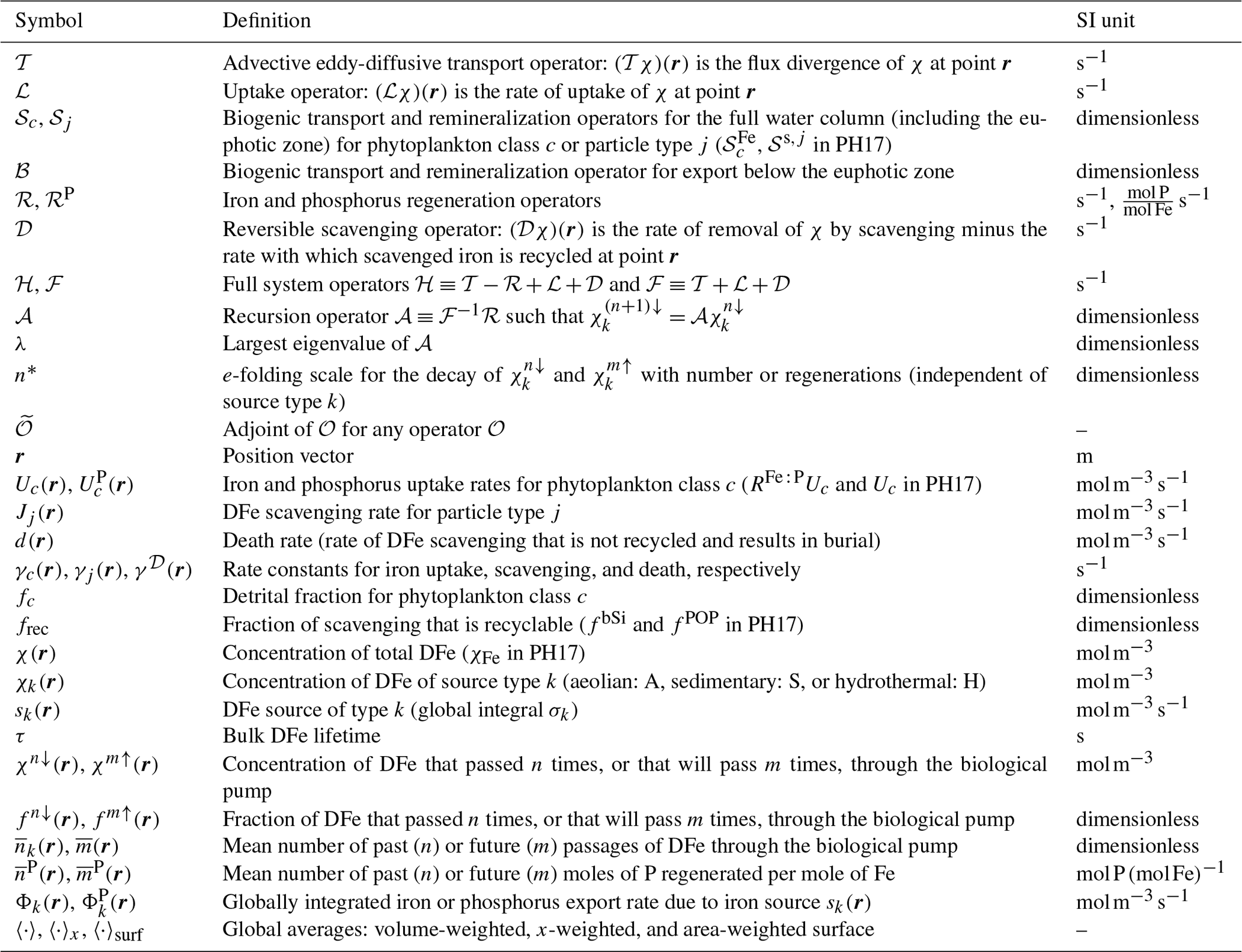
Table A1Glossary of mathematical symbols, their definitions, and SI units (PH17 refers to Pasquier and Holzer, 2017).
First we verify that . From Eqs. (4) and (5) we have
where . Because 𝒜 must have a maximum eigenvalue less than unity for convergence, we can use the geometric operator sum . Thus,
Applying ℱ(1−𝒜) from the left, and recognizing that , we have
This shows that and χk obey the same equation and hence that they are equal.
The defining equation for is
From recursion Eq. (5), we have . Substituting this, applying the geometric operator sum , and using the fact that from Eq. (B1) , we obtain
Applying from the left yields Eq. (6).
To diagnose the local death rate with which iron is permanently removed from the ocean, we first rewrite the reversible scavenging operator 𝒟 in terms of a simplified local death rate. The operator 𝒟 is an integral operator so that with adjoint . The term represents the rate with which iron is scavenged at r′ minus the rate with which this scavenged iron is redistributed to points r through particle transport and redissolution. By integrating over all destination points r, we obtain the deficit between the rate of iron scavenging at r′ and the total water-column-integrated rate of redissolution of that iron. Thus, is the rate of permanent removal or death at r′. For the local rate constant we define , which gives .
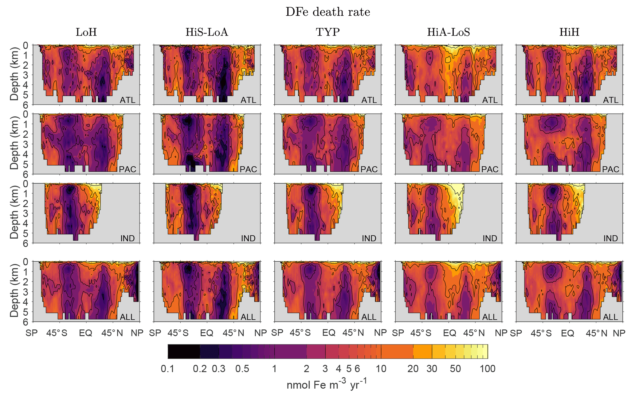
Figure C1Basin and global zonal averages of the death rate d(r′) for our five representative states. Note the logarithmic color scale.
For the interpretation of our diagnostics it is helpful to know how the local iron death rate d(r′) is distributed through the ocean. Figure C1 shows basin and global zonal averages of the death rate for our five representative states. Key features common to all states are relatively low death rates in the subtropical gyres of both hemispheres, where production and hence scavenging particle fluxes are low, and relatively high death rates at high latitudes and in the tropics where production is large. The highest death rates occur in the surface ocean where particle fluxes are highest. The near-surface death rates are larger in the Northern Hemisphere than in the Southern Hemisphere, presumably because the DFe concentrations are higher in the Northern Hemisphere.
To explore the sensitivity of our results to variations in frec, we changed the value of frec of our typical state (for which frec=90 %) and then re-optimized the biogeochemical sink and source parameters following the optimization strategy described by Pasquier and Holzer (2017). This generated a set of eight optimized state estimates with , and 100 %. Except for the frec=100 % case, these states have similar iron source strengths (σA ranges from 5.3 to 5.7 Gmol yr−1, σS from 1.7 to 1.9 Gmol yr−1, and σH is unchanged to two significant figures at 0.88 Gmol yr−1). For the extreme case of frec=100 %, when the only permanent iron sink in the system is due to the flux of scavenged iron that reaches the ocean bottom where we assume it is buried (in addition, iron scavenged by mineral dust is always assumed not to be recyclable, but dust scavenging is very small for our estimates), the optimized sedimentary iron source more than doubles and the other sources also undergo significant adjustments during the re-optimization (σA=5.1, σS=3.7, and σH=0.85 Gmol yr−1 for frec=100 %).
Figure D1 shows that the spatial pattern of the zonally averaged is very insensitive to the value of frec when the scavenging and source parameters are optimized. The patterns of the zonally averaged have the same qualitative features for all values of frec, but become more surface intensified as frec increases to unity, presumably because a greater recycling fraction increases the chance that DFe is available near the euphotic zone to pass through the biological pump. The patterns of and (not shown) are similarly insensitive to frec.
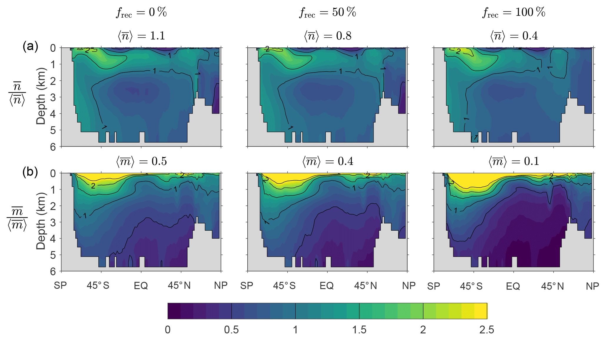
Figure D1(a) The zonal means of normalized by the corresponding global averages for our typical state estimate re-optimized with three very different recyclable fractions: and 100 %. (b) The corresponding normalized zonal means of . The values of the global averages, and , are given in the plot titles.
Figure D2 shows how the volume-weighted global means of , , , and vary with the recyclable fraction, frec. We find that and are order unity for frec=0 % and tend to decrease by roughly a factor of 2 to 3 when frec is increased from 0 to 100 %. We emphasize that this is not simple sensitivity to frec because the scavenging and source parameters have been re-optimized for each choice of frec. Broadly, a larger value of the number of regenerations means that more iron is transported to depth with the biological pump. This is consistent with the fact that for small values of frec, less iron is transported to depth through scavenging and redissolution. Given the similar iron sources of these states, and hence similar global mean scavenging rates, reduced iron transport through scavenging must be compensated for by increased transport through biological uptake and regeneration, as measured here by the mean number or iron regenerations. The mean numbers of phosphorus molecules that are regenerated in the past or the future per iron molecule, and , are much less sensitive to the value of frec in these optimized states. The reason for this insensitivity probably lies in the fact that the phosphorus export is well constrained by the nutrient and phytoplankton data against which we optimize (Pasquier and Holzer, 2017), and any changes in iron export are compensated for by different optimized values of the Fe : P uptake ratio, which we also use as the Fe : P ratio for remineralization.
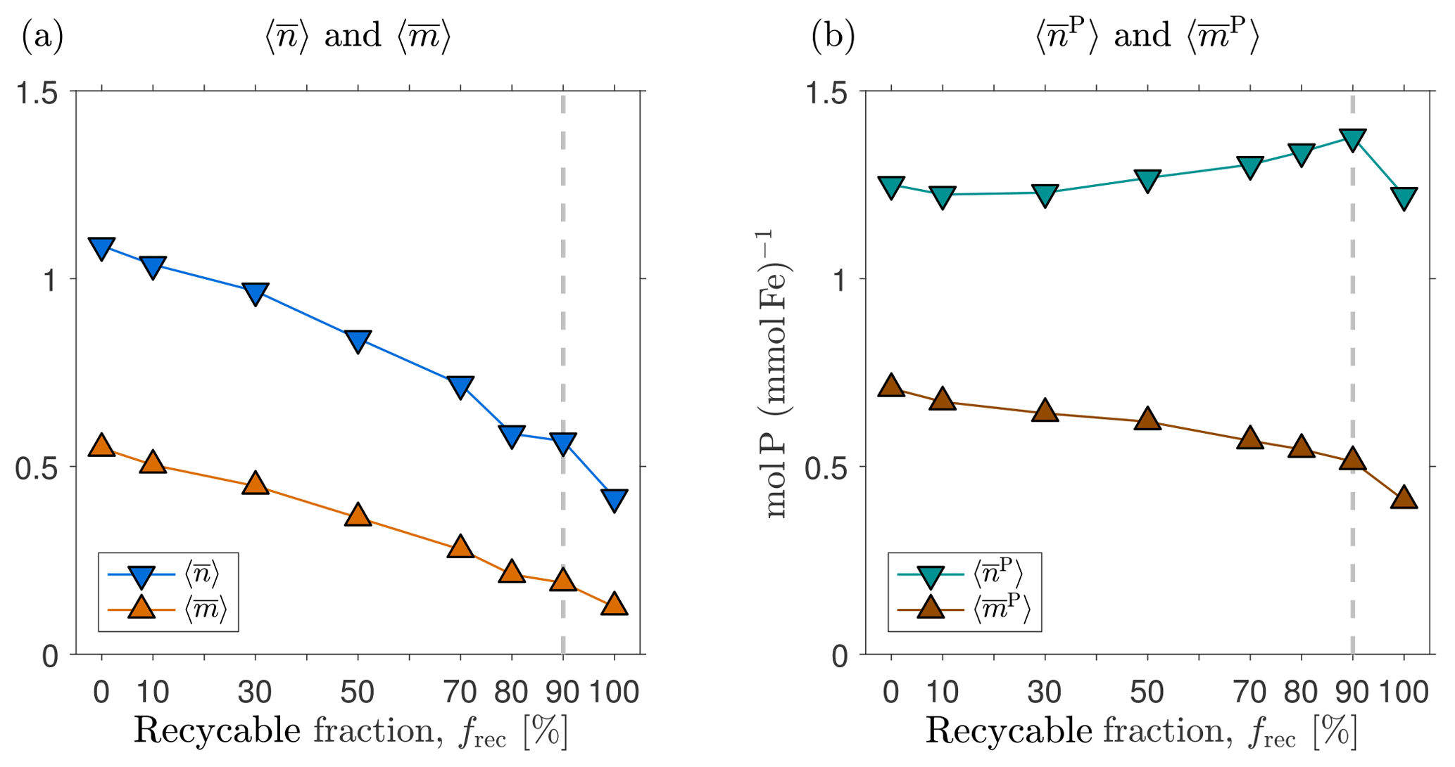
Figure D2(a) The globally averaged mean number of past and future DFe regenerations per injected DFe molecule, and , as a function of the recyclable fraction frec. The corresponding states were obtained by changing the value of frec of the typical state and re-optimizing all other source and scavenging parameters. The typical state has frec = 90 % and is indicated by the vertical dashed line. Panel (b) is the same as panel (a) but for the past and future number of phosphorus molecules exported per injected DFe molecule, and .
E1 Green functions
To derive the recursion relation for the fraction of iron at a given location that is regenerated exactly m times before death, we use a Green function approach. The Green function associated with the equation is obtained by replacing the source s with a Dirac delta function in space and time:
where the subscript on ℋr reminds us that ℋ acts on the field-point coordinates r. The Green function for the time-reversed adjoint flow (Holzer and Hall, 2000) obeys
where the adjoint Green function obeys the reciprocity relation . The Green functions associated with are defined in exactly the same manner.
All adjoints here are defined in terms of the volume-weighted inner product so that for linear operator ℋ and any two fields x and y we have . For computation, all linear operators are discretized on a numerical grid and organized into sparse matrices; e.g., ℋ becomes matrix H with adjoint , where V is a diagonal matrix of the grid box volumes.
E2 All DFe must die
Now consider the concentration of iron in some volume d3r′. As the system evolves the mass results in concentration at (r,t), which is obtained by propagating with Gℋ so that
(Note that there is no integral as this is point-wise propagation.) The death rate per unit volume incurred by at (r,t) is given by . Integrating this death rate over all times t and over the entire ocean for r, we must recover the initial mass . Thus, we have
where the initial volume d3r′ is not integrated over. Because Gℋ is just a function and not a differential operator, and because we are integrating with respect to (r,t), we can divide both sides by , which gives
where f↑ is just a spatially uniform field of unit value, i.e., . Applying the time-reversed adjoint operator from the left to Eq. (E5) and using the reciprocity relation of Gℋ, we obtain Eq. (8). Note that . Because 𝒯 and ℒ−ℛ are mass-conserving operators, and so that Eq. (8) is equivalent to , which reproduces the definition of γ𝒟.
E3 Fraction not regenerated in the future
Similarly we can construct the concentration of DFe that has been regenerated exactly zero times since being at . By propagating the mass with ℱ instead of ℋ, we obtain the resulting concentration at t that has not passed through the biological pump since t′:
Calculating the death rate per unit volume by multiplying with γ𝒟 and integrating over all r and t must give the mass in d3r′ that will not be regenerated in the future, i.e., . Dividing both sides by the starting mass and defining the fraction gives
Applying the time-reversed adjoint operator from the left gives Eq. (9).
Recursion for the fraction regenerated m times in the future
To construct the recursion equation for fm↑, it is useful to explicitly write the regeneration operator in terms of its integration kernel:
We again consider the concentration at (r,t) resulting from the mass of DFe in d3r′ at t′ that was not regenerated since t′, , as defined by Eq. (E6). The rate with which is regenerated (i.e., remineralized) in volume is given by (where d3r′ is not integrated over) and the fraction of this rate that will get regenerated a further m times in the future is given by
Integrating this rate over all and t, we must recover the fraction of the initial mass at t′ that will be regenerated exactly m+1 times in the future. Hence, we have
Dividing both sides by the initial mass and with the adjoint regeneration operator defined through , where , we have
Note that Eq. (E11) propagates the fraction to be regenerated m times through one regeneration (modeled as instantaneous) and through the adjoint flow backward in time to the fraction that will be regenerated (m+1) times. Applying from the left gives the recursion Eq. (10). Note that this recursion equation can be written as . Using Eq. (9) and regrouping the factors of , this recursion relation can be rewritten as
where as in Appendix B, with adjoint . Equation (E12) is the analog of Eq. (B1) for the time-reversed adjoint problem.
Using similar techniques as in Appendix B, it follows readily that , as must be the case. Equation (11) for is also derived analogously to in Appendix B.
Here we calculate the steady-state globally integrated export that results from a steady injection with source s(r′) (in ) in some volume d3r′ during dt′. Propagating the initial DFe mass with ℋ results in concentration at (r,t). This DFe is instantly regenerated at with rate . Integrating over all and t must give the globally integrated export that is due to the initial injection of the mass , and further dividing by gives
The globally integrated export per unit source injection at r′ is thus . Dividing Eq. (F1) by s(r′) and applying gives
which is the Green function that propagates a unit source to globally integrated export. Comparison with Eq. (11) shows that from which Eq. (13) of the main text follows by replacing our generic source s(r′) with one of the sources sk(r′). Equation (14) for the global phosphorus export due to DFe injection at r′ can be derived in exactly the same way by using regeneration operator ℛP instead of ℛ.
The authors declare that they have no conflict of interest.
Benoît Pasquier acknowledges support from the Government of Monaco, the
Scientific Centre of Monaco, the Frères Louis et Max Principale
Foundation, the Cuomo Foundation, Jefferson Keith Moore (DOE grant DE-SC0016539 and
NSF grant 1658380), and François Primeau (NSF grant 1658380). Mark Holzer
acknowledges a UNSW Goldstar award.
Edited by: Jack Middelburg
Reviewed by:
Christoph Völker, Jonathan Lauderdale,
and one anonymous referee
Achterberg, E. P., Steigenberger, S., Marsay, C. M., LeMoigne, F. A. C., Painter, S. C., Baker, A. R., Connelly, D. P., Moore, C. M., Tagliabue, A., and Tanhua, T.: Iron Biogeochemistry in the High Latitude North Atlantic Ocean, Sci. Rep. UK, 8, 1283, https://doi.org/10.1038/s41598-018-19472-1, 2018. a
Aumont, O. and Bopp, L.: Globalizing results from ocean in situ iron fertilization studies, Global Biogeochem. Cy., 20, GB2017, https://doi.org/10.1029/2005GB002591, 2006. a, b, c
Boyd, P. W., Jickells, T., Law, C. S., Blain, S., Boyle, E. A., Buesseler, K. O., Coale, K. H., Cullen, J. J., de Baar, H. J. W., Follows, M., Harvey, M., Lancelot, C., Levasseur, M., Owens, N. P. J., Pollard, R., Rivkin, R. B., Sarmiento, J., Schoemann, V., Smetacek, V., Takeda, S., Tsuda, A., Turner, S., and Watson, A. J.: Mesoscale Iron Enrichment Experiments 1993–2005: Synthesis and Future Directions, Science, 315, 612–617, https://doi.org/10.1126/science.1131669, 2007. a, b
Boyd, P. W., Ellwood, M. J., Tagliabue, A., and Twining, B. S.: Biotic and abiotic retention, recycling and remineralization of metals in the ocean, Nat. Geosci., 10, 167–173, https://doi.org/10.1038/ngeo2876, 2017. a
Boyer, T. P., Antonov, J. I., Baranova, O. K., Coleman, C., Garcia, H. E., Grodsky, A., Johnson, D. R., Locarnini, R. A., Mishonov, A. V., O'Brien, T. D., Paver, C. R., Reagan, J. R., Seidov, D., Smolyar, I. V., and Zweng, M. M.: World Ocean Database 2013, NOAA Atlas NESDIS 72, edited by: Levitus, S., A. Mishonov, Technical Ed., Silver Spring, MD, 209 pp., https://doi.org/10.7289/V5NZ85MT, 2013.
Conway, T. M. and John, S. G.: Quantification of dissolved iron sources to the North Atlantic Ocean, Nature, 511, 212–215, https://doi.org/10.1038/nature13482, 2014. a
de Baar, H., Gerringa, L., Laan, P., and Timmermans, K.: Efficiency of carbon removal per added iron in ocean iron fertilization, Mar. Ecol. Prog. Ser., 364, 269–282, https://doi.org/10.3354/meps07548, 2008. a, b, c, d, e, f
DeVries, T., Primeau, F., and Deutsch, C.: The sequestration efficiency of the biological pump, Geophys. Res. Lett., 39, L13601, https://doi.org/10.1029/2012GL051963, 2012. a
Dutkiewicz, S., Follows, M. J., Heimbach, P., and Marshall, J.: Controls on ocean productivity and air-sea carbon flux: An adjoint model sensitivity study, Geophys. Res. Lett., 33, L02603, https://doi.org/10.1029/2005GL024987, 2006. a, b, c, d, e
Elrod, V. A., Berelson, W. M., Coale, K. H., and Johnson, K. S.: The flux of iron from continental shelf sediments: A missing source for global budgets, Geophys. Res. Lett., 31, L12307, https://doi.org/10.1029/2004GL020216, 2004. a
Fitzsimmons, J. N., John, S. G., Marsay, C. M., Hoffman, C. L., Nicholas, S. L., Toner, B. M., German, C. R., and Sherrell, R. M.: Iron persistence in a distal hydrothermal plume supported by dissolved–particulate exchange, Nat. Geosci., 10, 195–201, https://doi.org/10.1038/ngeo2900, 2017. a
Frants, M., Holzer, M., DeVries, T., and Matear, R.: Constraints on the Global Marine Iron Cycle from a Simple Inverse Model, J. Geophys. Res.-Biogeo., 121, 28–51, https://doi.org/10.1002/2015jg003111, 2016. a
Galbraith, E. D., Gnanadesikan, A., Dunne, J. P., and Hiscock, M. R.: Regional impacts of iron-light colimitation in a global biogeochemical model, Biogeosciences, 7, 1043–1064, https://doi.org/10.5194/bg-7-1043-2010, 2010. a
Holzer, M. and Hall, T. M.: Transit-time and tracer-age distributions in geophysical flows, J. Atmos. Sci., 57, 3539–3558, https://doi.org/10.1175/1520-0469(2000)057<3539:TTATAD>2.0.CO;2, 2000. a, b
Holzer, M., Primeau, F. W., DeVries, T., and Matear, R.: The Southern Ocean silicon trap: Data-constrained estimates of regenerated silicic acid, trapping efficiencies, and global transport paths, J. Geophys. Res.-Oceans, 119, 313–331, https://doi.org/10.1002/2013JC009356, 2014. a, b
Holzer, M., Frants, M., and Pasquier, B.: The age of iron and iron source attribution in the ocean, Global Biogeochem. Cy., https://doi.org/10.1002/2016GB005418, 2016. a, b
Kirchman, D. L.: Microbial ferrous wheel, Nature, 383, 303–304, https://doi.org/10.1038/383303a0, 1996. a
Kostadinov, T. S., Milutinovic, S., Marinov, I., and Cabré, A.: Size-partitioned phytoplankton carbon concentrations retrieved from ocean color data, links to data in NetCDF format, PANGAEA, https://doi.org/10.1594/PANGAEA.859005, 2016.
Luo, C., Mahowald, N., Bond, T., Chuang, P. Y., Artaxo, P., Siefert, R., Chen, Y., and Schauer, J.: Combustion iron distribution and deposition, Global Biogeochem. Cy., 22, GB1012, https://doi.org/10.1029/2007GB002964, 2008. a
Maldonado, M. T., Strzepek, R. F., Sander, S., and Boyd, P. W.: Acquisition of iron bound to strong organic complexes, with different Fe binding groups and photochemical reactivities, by plankton communities in Fe-limited subantarctic waters, Global Biogeochem. Cy., 19, GB4S23, https://doi.org/10.1029/2005GB002481, 2005. a
Martin, J. W., Knauer, G. A., Karl, D. M., and Broenkow, W. W.: VERTEX: Carbon cycling in the NE Pacific, Deep-Sea Res., 34, 267–285, 1987. a
Moore, J. K. and Braucher, O.: Sedimentary and mineral dust sources of dissolved iron to the world ocean, Biogeosciences, 5, 631–656, https://doi.org/10.5194/bg-5-631-2008, 2008. a, b
Mawji, E. et al.: The GEOTRACES Intermediate Data Product 2014, Mar. Chem., https://doi.org/10.1016/j.marchem.2015.04.005, 2015.
NASA (Goddard Space Flight Center, Ocean Ecology Laboratory) Ocean Biology Processing Group: Moderate-resolution Imaging Spectroradiometer (MODIS) Aqua Chlorophyll Data, 2014 Reprocessing, NASA OB.DAAC, Greenbelt, MD, USA, https://doi.org/10.5067/AQUA/MODIS/L3B/CHL/2014, 2014.
Pasquier, B. and Holzer, M.: The plumbing of the global biological pump: Efficiency control through leaks, pathways, and time scales, J. Geophys. Res.-Oceans, 121, 6367–6388, https://doi.org/10.1002/2016JC011821, 2016. a
Pasquier, B. and Holzer, M.: Inverse-model estimates of the ocean's coupled phosphorus, silicon, and iron cycles, Biogeosciences, 14, 4125–4159, https://doi.org/10.5194/bg-14-4125-2017, 2017. a, b, c, d, e, f, g, h, i, j, k, l, m, n, o, p, q, r, s, t, u, v, w, x
Primeau, F. W., Holzer, M., and DeVries, T.: Southern Ocean nutrient trapping and the efficiency of the biological pump, J. Geophys. Res., 118, 2547–2564, https://doi.org/10.1002/jgrc.20181, 2013. a, b, c, d, e
Qin, X., Menviel, L., Gupta, A. S., and Sebille, E.: Iron sources and pathways into the Pacific Equatorial Undercurrent, Geophys. Res. Lett., 43, 9843–9851, https://doi.org/10.1002/2016GL070501, 2016. a
Rafter, P. A., Sigman, D. M., and Mackey, K. R. M.: Recycled iron fuels new production in the eastern equatorial Pacific Ocean, Nat. Commun., 8, 1100, https://doi.org/10.1038/s41467-017-01219-7, 2017. a
Raven, J. A.: The iron and molybdenum use efficiencies of plant growth with different energy, carbon and nitrogen sources, New Phytol., 109, 279–287, https://doi.org/10.1111/j.1469-8137.1988.tb04196.x, 1988. a
Strzepek, R. F., Maldonado, M. T., Higgins, J. L., Hall, J., Safi, K., Wilhelm, S. W., and Boyd, P. W.: Spinning the “Ferrous Wheel”: The importance of the microbial community in an iron budget during the FeCycle experiment, Global Biogeochem. Cy., 19, GB4S26, https://doi.org/10.1029/2005GB002490, 2005. a
Tagliabue, A., Mtshali, T., Aumont, O., Bowie, A. R., Klunder, M. B., Roychoudhury, A. N., and Swart, S.: A global compilation of dissolved iron measurements: focus on distributions and processes in the Southern Ocean, Biogeosciences, 9, 2333–2349, https://doi.org/10.5194/bg-9-2333-2012, 2012. a
Tagliabue, A., Williams, R. G., Rogan, N., Achterberg, E. P., and Boyd, P. W.: A ventilation-based framework to explain the regeneration-scavenging balance of iron in the ocean, Geophys. Res. Lett., 41, 7227–7236, https://doi.org/10.1002/2014GL061066, 2014GL061066, 2014. a
Tagliabue, A., Aumont, O., DeAth, R., Dunne, J. P., Dutkiewicz, S., Galbraith, E., Misumi, K., Moore, J. K., Ridgwell, A., Sherman, E., Stock, C., Vichi, M., Völker, C., and Yool, A.: How Well do Global Ocean Biogeochemistry Models Simulate Dissolved Iron Distributions?, Global Biogeochem. Cy., 30, 149–174, https://doi.org/10.1002/2015gb005289, 2016. a, b
Twining, B. S., Nodder, S. D., King, A. L., Hutchins, D. A., LeCleir, G. R., DeBruyn, J. M., Maas, E. W., Vogt, S., Wilhelm, S. W., and Boyd, P. W.: Differential remineralization of major and trace elements in sinking diatoms, Limnol. Oceanogr., 59, 689–704, https://doi.org/10.4319/lo.2014.59.3.0689, 2014. a
Zeebe, R. E. and Archer, D.: Feasibility of ocean fertilization and its impact on future atmospheric CO2 levels, Geophys. Res. Lett., 32, L09703, https://doi.org/10.1029/2005GL022449, 2005. a, b, c, d, e
- Abstract
- Introduction
- Iron model
- Past contributions to export
- Future contributions to export
- Intrinsic iron fertilization efficiencies
- Discussion and caveats
- Conclusions
- Data availability
- Appendix A
- Derivation of
- Appendix C: Local iron death rate
- Appendix D: Variation of key diagnostics with recyclable fraction parameter
- Recursion relation for fm↑
- Relation between export and
- Competing interests
- Acknowledgements
- References