the Creative Commons Attribution 4.0 License.
the Creative Commons Attribution 4.0 License.
 | 22 Nov 2018
Factors controlling coccolithophore biogeography in the Southern Ocean
Meike Vogt
Matthias Münnich
Nicolas Gruber
F. Alexander Haumann
The biogeography of Southern Ocean phytoplankton controls the local biogeochemistry and the export of macronutrients to lower latitudes and depth. Of particular relevance is the competitive interaction between coccolithophores and diatoms, with the former being prevalent along the “Great Calcite Belt” (40–60∘ S), while diatoms tend to dominate the regions south of 60∘ S. To address the factors controlling coccolithophore distribution and the competition between them and diatoms, we use a regional high-resolution model (ROMS–BEC) for the Southern Ocean (24–78∘ S) that has been extended to include an explicit representation of coccolithophores. We assess the relative importance of bottom-up (temperature, nutrients, light) and top-down (grazing by zooplankton) factors in controlling Southern Ocean coccolithophore biogeography over the course of the growing season. In our simulations, coccolithophores are an important member of the Southern Ocean phytoplankton community, contributing 17 % to annually integrated net primary productivity south of 30∘ S. Coccolithophore biomass is highest north of 50∘ S in late austral summer, when light levels are high and diatoms become limited by silicic acid. Furthermore, we find top-down factors to be a major control on the relative abundance of diatoms and coccolithophores in the Southern Ocean. Consequently, when assessing potential future changes in Southern Ocean coccolithophore abundance, both abiotic (temperature, light, and nutrients) and biotic factors (interaction with diatoms and zooplankton) need to be considered.
- Article
(5338 KB) -
Supplement
(6572 KB) - BibTeX
- EndNote


The ocean is changing at an unprecedented rate as a consequence of increasing anthropogenic CO2 emissions and related climate change. Changes in density stratification and nutrient supply, as well as ocean acidification, lead to changes in phytoplankton community composition and consequently ecosystem structure and function. Some of these changes are already observable today (Soppa et al., 2016; Winter et al., 2013) and may have cascading effects on global biogeochemical cycles and oceanic carbon uptake (Cermeño et al., 2008; Freeman and Lovenduski, 2015; Laufkötter et al., 2016). Changes in Southern Ocean (SO) biogeography are especially critical due to the importance of the SO in fueling primary production at lower latitudes through the lateral export of nutrients (Sarmiento et al., 2004) and in taking up anthropogenic CO2 (Frölicher et al., 2015). For the carbon cycle, the ratio of calcifying and noncalcifying phytoplankton is crucial due to the counteracting effects of calcification and photosynthesis on seawater pCO2, which ultimately controls CO2 exchange with the atmosphere, and the differing ballasting effect of calcite and silicic acid shells for organic carbon export.
Calcifying coccolithophores and silicifying diatoms are globally ubiquitous phytoplankton functional groups (Leblanc et al., 2012; O'Brien et al., 2013). Diatoms are a major contributor to global phytoplankton biomass (Buitenhuis et al., 2013b) and annual net primary production (Sarthou et al., 2005). In comparison, coccolithophores contribute less to biomass (Buitenhuis et al., 2013b) and to global NPP (Gregg and Casey, 2007a; Jin et al., 2006; Moore et al., 2004; O'Brien, 2015). However, coccolithophores are the major phytoplanktonic calcifier (Iglesias-Rodríguez et al., 2002), thereby significantly impacting the global carbon cycle. Diatoms dominate the phytoplankton community in the SO (Swan et al., 2016; Trull et al., 2018; Wright et al., 2010), but coccolithophores have received increasing attention in recent years. Satellite imagery of particulate inorganic carbon (PIC, a proxy for coccolithophore abundance) revealed the “Great Calcite Belt” (Balch et al., 2011), an annually reoccurring circumpolar band of elevated PIC concentrations between 40 and 60∘ S. In situ observations confirmed coccolithophore abundances of up to 2.4×10³ cells mL−1 in the Atlantic sector (blooms on the Patagonian Shelf), up to 3.8×10² cells mL−1 in the Indian sector (Balch et al., 2016), and up to 5.4×10² cells mL−1 in the Pacific sector of the SO (Cubillos et al., 2007) with Emiliania huxleyi being the dominant species (Balch et al., 2016; Saavedra-Pellitero et al., 2014). However, the contribution of coccolithophores to total SO phytoplankton biomass and NPP has not yet been assessed. Locally, elevated coccolithophore abundance in the GCB has been found to turn surface waters into a source of CO2 for the atmosphere (Balch et al., 2016), emphasizing the necessity to understand the controls on their abundance in the SO in the context of the carbon cycle and climate change. While coccolithophores have been observed to have moved polewards in recent decades (Beaugrand et al., 2012; Rivero-Calle et al., 2015; Winter et al., 2013), their response to the combined effects of future warming and ocean acidification is still subject to debate (Beaufort et al., 2011; Beaugrand et al., 2012; Iglesias-Rodríguez et al., 2008; Riebesell et al., 2000; Schlüter et al., 2014). As their response will also crucially depend on future phytoplankton community composition and predator–prey interactions (Dutkiewicz et al., 2015), it is essential to assess the controls on their abundance in today's climate.
Coccolithophore biomass is controlled by a combination of bottom-up (physical–biogeochemical environment) and top-down factors (predator–prey interactions), but the relative importance of the two has not yet been assessed for coccolithophores in the SO. Bottom-up factors directly impact phytoplankton growth, and diatoms and coccolithophores are traditionally discriminated based on their differing requirements for nutrients, turbulence, and light. Based on this, Margalef's mandala predicts a seasonal succession from diatoms to coccolithophores as light levels increase and nutrient levels decline (Margalef, 1978). In situ studies assessing SO coccolithophore biogeography have found coccolithophores under various environmental conditions (Balch et al., 2016; Charalampopoulou et al., 2016; Hinz et al., 2012; Saavedra-Pellitero et al., 2014; Trull et al., 2018), thus suggesting a wide ecological niche, but all of the mentioned studies have almost exclusively focused on bottom-up controls.
However, phytoplankton growth rates do not necessarily covary with biomass accumulation rates. Using satellite data from the North Atlantic, Behrenfeld (2014) stresses the importance of simultaneously considering bottom-up and top-down factors when assessing seasonal phytoplankton biomass dynamics and the succession of different phytoplankton types owing to the spatially and temporally varying relative importance of the physical–biogeochemical and the biological environment. In the SO, previous studies have shown zooplankton grazing to control total phytoplankton biomass (Le Quéré et al., 2016), phytoplankton community composition (Granéli et al., 1993), and ecosystem structure (De Baar, 2005; Smetacek et al., 2004), suggesting that top-down control might also be an important driver for the relative abundance of coccolithophores and diatoms. But the role of zooplankton grazing in current Earth system models is not well considered (Hashioka et al., 2013; Sailley et al., 2013), and the impact of different grazing formulations on phytoplankton biogeography and diversity is subject to ongoing research (Prowe et al., 2012; Vallina et al., 2014).
While none of the SO in situ studies directly assessed interactions of diatoms and coccolithophores over the course of the year, some in situ studies infer a diatom–coccolithophore succession from depleted silicic acid coinciding with iron levels high enough to sustain elevated coccolithophore abundance (Balch et al., 2014, 2016; Painter et al., 2010). In contrast to this, recent in situ and satellite studies find coccolithophores and diatoms to coexist rather than succeed each other throughout the growth season in the North Atlantic (Daniels et al., 2015) and the global open ocean (Hopkins et al., 2015). In fact, large areas of the GCB have been identified as “coexistence” areas (Hopkins et al., 2015), thereby putting into question the succession pattern predicted by Margalef's mandala (Margalef, 1978) and results of in situ studies for the SO (Balch et al., 2014, 2016; Painter et al., 2010). This highlights the necessity to better understand the drivers and seasonal dynamics of the relative importance of coccolithophores and diatoms in the SO before assessing potential future changes.
In this study, we use a regional high-resolution model for the SO to simultaneously assess the relative importance of bottom-up versus top-down factors in controlling SO coccolithophore biogeography over a complete annual cycle. In particular, we assess the role of diatoms in constraining high coccolithophore abundance and the importance of microzooplankton and macrozooplankton grazing for the relative importance of coccolithophores and diatoms in the GCB area.
2.1 Model description: ROMS–BEC with explicit coccolithophores
We use a regional, circumpolar SO setup of the UCLA-ETH version of the Regional Ocean Modeling System (Haumann, 2016; Shchepetkin and McWilliams, 2005) with a latitudinal range from ≈24–78∘ S and an open northern boundary. The primitive equations are solved on a curvilinear grid: the model setup has 64 topography-following vertical levels, its horizontal resolution for this study is (5.4–25.4 km), and the time step is 1600 s.
Coupled to this is an extended version of the ecosystem–biogeochemical model BEC (Moore et al., 2013) that we modified to include an explicit parameterization of coccolithophores and an updated formulation for sedimentary iron fluxes to allow for temporal and spatial variability of these fluxes (Dale et al., 2015). BEC resolves the cycling of carbon, nitrogen, phosphorus, silicon, and iron by simulating a total of 30 tracers. Besides explicit coccolithophores, it includes three phytoplankton plankton functional types (PFTs) (diatoms, a mixed small phytoplankton class (SP), N2-fixing diazotrophs) and one zooplankton PFT. Phytoplankton C ∕ N ∕ P stoichiometry in photosynthesis is fixed close to Redfield ratios (Anderson and Sarmiento, 1994; Letelier and Karl, 1998), but the ratios of Fe ∕ C, Si ∕ C, and Chl ∕ C vary according to surrounding nutrient levels. Detrital matter is split into a non-sinking and a sinking pool, with ballasting of the latter by atmospheric dust, biogenic silica, or calcium carbonate (Armstrong et al., 2002). Dissolved inorganic carbon (DIC) and alkalinity are included to complete the cycling of carbon in the model.
The phytoplankton PFTs differ with respect to their maximum growth rate (μmax), temperature (Q10) and light (αPI) sensitivities, half-saturation constants for nutrient uptake (k), and grazing preferences by zooplankton (γmax, Table 1). The SO coccolithophore community appears to mainly consist of the ubiquitous Emiliania huxleyi (Krumhardt et al., 2017; Saavedra-Pellitero et al., 2014) and parameter values used for coccolithophores here are based on available data for this species in the literature, both from in situ and laboratory studies (Buitenhuis et al., 2008; Daniels et al., 2014; Heinle, 2013; Le Quéré et al., 2016; Nielsen, 1997; Zondervan, 2007). Based on the available information, parameter values for coccolithophores lie between those of diatoms and SP (Table 1). Due to their smaller size, coccolithophores are less nutrient limited at low nutrient concentrations (smaller half-saturation constants, Eppley et al., 1969) and have a smaller maximum growth rate than diatoms (Buitenhuis et al., 2008). Coccolithophores grow well at high light intensities, but have been shown to be light inhibited at low light levels (Zondervan, 2007). In addition, they tend to reduce their growth at low temperatures (Buitenhuis et al., 2008). For this study, we use a constant calcite-to-organic-matter (CaCO3 : Corg) production ratio for coccolithophores of 0.2 (Müller et al., 2015). Previous work has shown this ratio to vary from 0.1–0.3 across environmental conditions for the SO morphotype of Emiliania huxleyi (Krumhardt et al., 2017), and we assess the sensitivity of integrated annual calcification estimates to this ratio in Sect. 4.2.
Table 1The most relevant BEC parameters for this study as used in the reference run (see Sect. 2.2) for the four phytoplankton PFTs coccolithophores (C), diatoms (D), small phytoplankton (SP), and diazotrophs (N). Z: zooplankton, P: phytoplankton, PI: photosynthesis–irradiance.
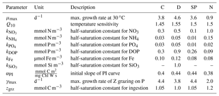
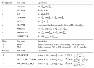
Table 2Overview of sensitivity simulations. 1–9: sensitivity of simulated coccolithophore–diatom competition to chosen parameter values of coccolithophores. See Table 1 for parameter values of coccolithophores in the reference run. 10–11: sensitivity of simulated biogeography to biases in temperature and mixed layer depth. 12–14: sensitivity of simulated biogeography to the chosen grazing formulation. C: coccolithophores, D: diatoms.
In BEC, phytoplankton are grazed by a single zooplankton PFT comprising characteristics of both microzooplankton and macrozooplankton (Moore et al., 2002; Sailley et al., 2013). The single zooplankton PFT grazes on all phytoplankton PFTs using a Holling type II ingestion function (Holling, 1959). This is in contrast to earlier versions of BEC, wherein a Holling type III ingestion function was used (Moore et al., 2002). While not explicitly stated in the published literature, the formulation was already changed to a Holling type II ingestion function in previous, more recent applications of BEC (Matthew Long, personal communication, 2018; Moore et al., 2013). Microzooplankton exert the biggest grazing pressure on coccolithophores, possibly mainly through nonselective grazing for species like Emiliania huxleyi (Monteiro et al., 2016). In BEC, we assign the same maximum zooplankton growth rate (γmax, Table 1) for feeding on SP and coccolithophores, thereby assuming that only differences in their absolute biomass concentrations leads to differences in grazing pressure, not the absence or presence of a coccosphere. In contrast, diatoms are mainly grazed by larger, slower-growing macrozooplankton (lower γmax, Table 1). A full description of the model equations regarding phytoplankton growth and loss terms can be found in Sect. 3 and in Appendix B.
Table 3Comparison of ROMS–BEC-based phytoplankton biomass, production, calcification, and export estimates with available observations (given in parentheses). See Appendix Table A1 for data sources.
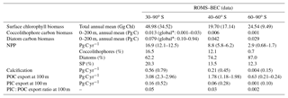
* The reported estimates from the MAREDAT database in Buitenhuis et al. (2013b) are global estimates of phytoplankton biomass.
2.2 Model setup and baseline simulation
At the surface, ROMS–BEC is forced by daily fluxes of momentum, heat, and freshwater constructed from ERA-Interim data (Dee et al., 2011). These fluxes are obtained by first calculating monthly climatological fluxes from 1979–2014 and then adding daily anomalies of the year 2003 to account for higher-frequency variability. The surface freshwater flux is corrected for river runoff, sea ice formation, and melting (Haumann, 2016), and dust deposition (Mahowald et al., 2009) is scaled by the monthly climatological sea ice cover.
At the open northern boundary, the model is forced with monthly climatological fields for all tracers. Current velocities are taken from SODA (Carton and Giese, 2008), and temperature and salinity from WOA (Locarnini et al., 2013; Zweng et al., 2013). For BEC, WOA data are used for macronutrients (Garcia et al., 2014a) and oxygen (Garcia et al., 2014b), and GLODAP data for DIC and alkalinity (Lauvset et al., 2016). Dissolved iron, ammonium and dissolved organic carbon, nitrogen, phosphorus, and iron fields are from climatological model output from the global model CESM-BEC (Yang et al., 2017). Phytoplankton chlorophyll biomass fields are taken from a climatological surface chlorophyll field (NASA-OBPG, 2014b) using a constant partitioning of the different phytoplankton PFTs to total chlorophyll everywhere at the boundary (SP: 90 %, diatoms: 4.5 %, coccolithophores: 4.5 %, diazotrophs: 1 %) and then extrapolating to depth according to Morel and Berthon (1989). Phytoplankton carbon biomass fields are then derived using a constant carbon-to-chlorophyll ratio of 36 mg C (mg Chl)−1 for diatoms and 60 mg C (mg Chl)−1 for all other PFTs (Sathyendranath et al., 2009). To minimize model drift in the physical parameters, sea surface temperature (Reynolds et al., 2007) and salinity (Good et al., 2013) fields are restored wherever sea ice is absent, with a restoring timescale of 45 days for salinity and a spatially and temporally varying sensitivity of the surface heat flux to sea surface temperatures (Haumann, 2016). No restoring is applied to the biogeochemical tracers.
The model is first spun up from rest for velocity in a physics-only setup for 30 years and subsequently for another 10 years in the coupled ROMS–BEC setup. All tracers are initialized using the same data sources for initial fields as used for the lateral boundary forcing. The reference simulation analyzed in this study is run for 10 years after the coupled ROMS–BEC spin-up, of which only a daily climatology of the last 5 years is analyzed. To capture five full seasonal cycles at high southern latitudes, we calculate the climatology from 1 July of year 5 until 30 June of year 10 of the simulation. Ultimately, we focus the analysis in this study on the area south of 30∘ S to minimize potential effects of the open northern boundary on biomass distributions.
2.3 Sensitivity simulations
We perform a set of sensitivity simulations to assess the sensitivity of SO coccolithophore biogeography to choices of model parameters, parameterizations, and biases in the physical fields (Table 2). We conduct 14 simulations grouped into three sets: first, we adjust each of the coccolithophore parameters step by step to the corresponding diatom value (runs 1–9). Thereby, we can directly assess the impact of differences between coccolithophores and diatoms in each of the model parameters on the relative biomass of coccolithophores. For all simulations, we quantify the sensitivity as a change in each PFT's annual mean surface biomass, focusing particularly on coccolithophores in Sect. 4.7.
Second, we performed two additional sensitivity simulations (runs 10 and 11 in Table 2) to assess the effect of biases in the physical fields (temperature and mixed layer depth) on coccolithophore biogeography. To do this, we reduce temperatures by 1 ∘C (corresponding to the mean bias between 60 and 90∘ S; see Supplement Fig. S1, run 10) and the incoming PAR field by 20 % (to counteract bias in MLD, run 11) everywhere for the biological subroutine only.
Third, we assess the sensitivity of the results to the chosen grazing formulation by performing three additional simulations: we first replace the Holling type II ingestion term (Eq. 5) with a Holling type III term (Holling, 1959). Thereby, the grazing pressure is decreased on prey in low concentrations. We then assess the impact of constraining grazing on each phytoplankton PFT by total phytoplankton biomass in the original Holling type II formulation (Eq. 5). To do so, we first scale the grazing rate on phytoplankton i linearly with the PFT's relative contribution to total phytoplankton biomass (run 13) and ultimately constrain the grazing rate on phytoplankton i by total phytoplankton biomass in the Holling type II ingestion function (run 14). Similarly to the simulation using a Holling type III ingestion term, we expect the less abundant PFTs to profit most in both of these simulations, as relatively more of the total grazing pressure acts on the most abundant PFT (Vallina et al., 2014).
All sensitivity runs start from the common spin-up described in Sect. 2.2 and only differ in their respective settings within BEC (Table 2). As for the control run, each simulation is run for 10 years of which the average over the last 5 years is analyzed.
To disentangle the effect of the different controlling factors, relative growth and grazing ratios are computed as introduced by Hashioka et al. (2013) and outlined in the following. In BEC, phytoplankton biomass Pi (in mmol C m−3, ) is the balance of growth (μi) and loss terms (grazing by zooplankton , non-grazing mortality , and aggregation ; see Appendix B for a full description of the model equations regarding phytoplankton growth and loss terms):
with the specific phytoplankton growth μi (d−1) being dependent on the maximum growth rate (d−1; Table 1), temperature (fi(T), Eq. B5), nutrient availability (gi(N), Eq. B8; nitrate, ammonium, phosphorus, and iron for all PFTs, silicic acid for diatoms only), and light levels (hi(I), Eq. B9; following the growth model by Geider et al., 1998):
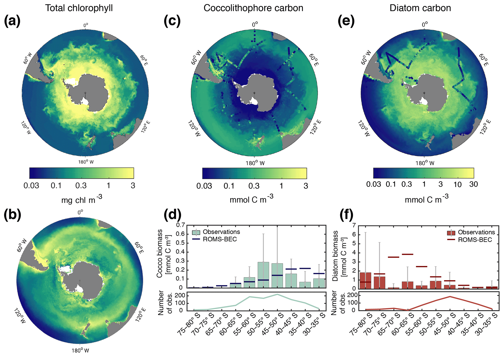
Figure 1Biomass distributions for December–March (DJFM). Total surface chlorophyll (mg Chl m−3) in (a) ROMS–BEC and (b) MODIS Aqua climatology (NASA-OBPG, 2014a) using the chlorophyll algorithm by Johnson et al. (2013). Mean top 50 m (c) coccolithophore and (e) diatom carbon biomass (mmol C m−3) in ROMS–BEC. Coccolithophore and diatom biomass observations from the top 50 m are indicated by colored dots in (c, e), respectively. (d, f) Mean top 50 m zonally averaged (d) coccolithophore and (f) diatom carbon biomass (mmol C m−3) binned into 5∘ latitudinal intervals for ROMS–BEC (line) and observations (bars). The grey bars denote the standard deviation of the observations. The lower panels show the number of observations used to obtain the bars in the respective upper panels. Note that (a)–(b) are on the same scale, while the scales in panels (c)–(f) are different. For more details on the biomass validation, see Table A1 and the Supplement.
The nondimensional relative growth ratio between two phytoplankton types i and j, e.g., diatoms and coccolithophores, can then be defined as the log of the ratio of their specific growth rates (Hashioka et al., 2013).
In this equation, the terms , βT, βN, and βI describe the log-transformed differences in the maximum growth rate μmax, temperature limitation f(T), nutrient limitation g(N), and light limitation h(I) between diatoms and coccolithophores, which in sum give the difference in the relative growth ratio . If is negative, the specific growth rate of coccolithophores is larger than that of diatoms and bottom-up factors promote the dominance of coccolithophores over diatoms (and vice versa). Based on the chosen parameter values for coccolithophores and diatoms in ROMS–BEC (see Sect. 2.1 and Table 1), coccolithophores grow better than diatoms when nutrient concentrations are low and irradiance is high (towards the end of the growth season). Simultaneously, coccolithophores are limited less by the ambient temperature than diatoms. Since the coccolithophore maximum growth rate is lower than that of diatoms (Table 1), ideal environmental conditions, i.e., low nutrient concentrations and temperature, and high light levels, are required for coccolithophores to overcome this disadvantage and to develop a higher specific growth rate than diatoms. Whether the resulting is positive or negative at any given location and point in time will depend on the complex interplay of the physical and biogeochemical environment at every location.
The specific grazing rate (mmol C m−3 d−1) of the generic zooplankton on the respective phytoplankton i is described by the Holling type II function:
with Z being zooplankton biomass (mmol C m−3), fZ(T) the temperature scaling function (Eq. B13), the maximum growth rate of zooplankton when feeding on phytoplankton i (d−1; Table 1), the respective half-saturation coefficient for ingestion (mmol C m−3; Table 1), and the phytoplankton biomass (mmol C m−3), which was corrected for a loss threshold below which no losses occur (prey refuge; Eq. B11).
To assess differences in biomass accumulation rates between different PFTs, we compute biomass-normalized specific grazing rates ci (d−1) of phytoplankton i as the ratio of the specific grazing rate and the respective phytoplankton's biomass Pi.
The higher this rate, the more difficult it is for a phytoplankton i to accumulate biomass. Consequently, the nondimensional relative grazing ratio of phytoplankton i and j, e.g., diatoms and coccolithophores, is defined as (Hashioka et al., 2013)
If is negative, the specific grazing rate on diatoms is larger than that on coccolithophores and grazing promotes the dominance of coccolithophores over diatoms (and vice versa). While the maximum grazing rate is larger on coccolithophores than on diatoms (see Sect. 2.1 and Table 1), the interplay with biomass concentrations at any given location and point in time will decide whether is positive or negative, i.e., whether the strength and direction of the grazing pressure favors coccolithophores or diatoms.
In contrast to Hashioka et al. (2013), who analyzed both the relative growth ratio and the relative grazing ratio as a function of the time of the annual maximum total chlorophyll concentration, we analyze them as a function of time to assess temporal variability in the controls on phytoplankton competition. We particularly focus on the interplay between coccolithophores and diatoms, as maximum coccolithophore abundance in the SO may be facilitated by declining diatom abundance (Balch et al., 2014).
4.1 Model evaluation
Phytoplankton growth directly responds to the physical and biogeochemical environment (Eq. 3), which is why systematic biases in the underlying bottom-up factors have to be assessed to understand biases in simulated phytoplankton biogeography and phenology. The data sets used for the model evaluation are presented in Table A1, and a more detailed description is found in the Supplement. Please see the “Data availability” section and Nissen et al. (2018) for model output.
In ROMS–BEC, SST is on average 0.9 ∘C and 0.2 ∘C too high and the ML is 1 m and 5 m too shallow in austral summer south and north of 60∘ S, respectively (Fig. S1), leading to an overestimation of phytoplankton growth (Figs. S1–S3). Macronutrients in ROMS–BEC are generally too low at the surface compared to WOA data (especially south of 60∘ S; Figs. S1 and S2), caused either by too much nutrient uptake by phytoplankton, too little nutrient supply from below, or both.
Total SO summer surface chlorophyll in ROMS–BEC reproduces the general south–north gradient as detected by remote sensing (Fig. 1a and b), with highest values above 10 mg Chl m−3 in our model in areas close to the Antarctic continent and lower concentrations of around 0.1 mg Chl m−3 north of 40∘ S. However, integrated over 30–90∘ S, ROMS–BEC overestimates annual mean satellite-derived surface chlorophyll biomass estimates by 42 % (49 Gg Chl in ROMS–BEC compared to 34.5 Gg Chl in satellite product; Table 3 and Fig. S2) and satellite-derived NPP by 35.2 %–40 % (16.9 compared to 12.1–12.5 Pg C yr−1; Table 3 and Figs. S2 and S3). This overestimation is mainly driven by the area south of 60∘ S (NPP and surface chlorophyll are overestimated by a factor of 2–4 and 2.5, respectively), while between 40 and 60∘ S, surface chlorophyll biomass is overestimated by only 15 % (Table 3 and Fig. S2).
The overestimation of phytoplankton production can at least partly be attributed to biases in SST and MLD, promoting phytoplankton growth (see also the discussion Sect. 5.4). However, data coverage south of 60∘ S, an area almost completely covered by sea ice every year, is low (Holte et al., 2017), impeding the assessment of model performance and the attribution of the bias in both production and biomass to underlying physical fields in this area. Additionally, satellite-derived surface chlorophyll and NPP fields are known to be associated with significant errors in high latitudes due to low sun elevation, clouds, or sea ice cover, complicating model assessment (Gregg and Casey, 2007b). In addition to the underlying physical and biogeochemical fields, phytoplankton biomass is also controlled by loss rates (Eq. 2). Since the overestimation of production between 40 and 60∘ S in ROMS–BEC compared to satellite-derived estimates is higher than the overestimation of surface chlorophyll biomass, phytoplankton losses in the area are probably overestimated (see also the discussion Sect. 5.4).
4.2 Quantifying the importance of SO coccolithophores for biogeochemical cycles
Our simulations with ROMS–BEC yield an annual mean SO coccolithophore carbon biomass within the top 200 m of 0.013 Pg C (Table 3). This is within the globally estimated range based on in situ observations (O'Brien et al., 2013) and suggests that SO coccolithophores contribute substantially to global coccolithophore biomass. Total simulated NPP south of 30∘ S is 16.9 Pg C yr−1 with diatoms contributing 62.2 %, small phytoplankton 20.3 %, coccolithophores 16.5 %, and diazotrophs 1 %. Compared to previous global estimates, annual coccolithophore NPP south of 30∘ S alone (2.8 Pg C yr−1) accounts for 4.3 %–5.5 % of total global NPP (58±7 Pg C yr−1; Buitenhuis et al., 2013a). Modeled integrated calcification amounts to 0.56 Pg C yr−1 south of 30∘ S (using a CaCO3 : Corg production ratio of 0.2 for coccolithophores). Applying the full experimental range of CaCO3 : Corg production ratios of SO Emiliania huxleyi (Krumhardt et al., 2017), and accounting for the relative error associated with the satellite calcification estimate (Balch et al., 2007), the model estimate (0.28–0.84 Pg C yr−1) falls within the range estimated from satellite observations (0.64–0.94 Pg C yr−1, obtained using Eq. (1) in Balch et al. (2007) with satellite sea surface temperature, chlorophyll, and PIC concentrations from NASA OBPG (2014a, c, d); see Sect. S1 in the Supplement). Compared to global satellite-derived estimates, the simulated calcification estimate south of 30∘ S accounts for 24 % (9.8 %–43.1 %) of global calcification.
The ratio of particulate inorganic (calcite) to organic carbon exported to depth (PIC : POC ratio, typically reported at depths of ≈100 m) is important for the long-term fate of atmospheric CO2. In ROMS–BEC, PIC and POC exports south of 30∘ S are 0.16 Pg C yr−1 and 3.08 Pg C yr−1, respectively. Accounting for the uncertainty in the CaCO3 : Corg production ratio of coccolithophores (Krumhardt et al., 2017), the average PIC : POC export ratio is 0.05 (0.03–0.08), which is in the same range as previously estimated for the global mean export ratio (Sarmiento et al., 2002). The simulated PIC : POC export ratios are highest on the Patagonian Shelf (0.04–0.11 for the annual mean, 0.05–0.15 for summer mean only; not shown) where coccolithophore biomass is highest (see Sect. 4.3), consistent with the elevated PIC : POC export ratios reported for this area (Balch et al., 2016).

Figure 2(a) Spatial distribution of phytoplankton communities in ROMS–BEC: diatom-dominated phytoplankton community vs. mixed communities with substantial contributions of coccolithophores and small phytoplankton. Communities in which neither coccolithophores (c) nor diatoms (d) contribute >20 % and (blue) >80 % (red), respectively, to total annual NPP are classified as mixed communities (grey). (b–c) Annual mean most limiting nutrient for (b) coccolithophore and (c) diatom growth rates at the surface. For small phytoplankton, the nutrient limitation pattern south of 40∘ S is generally the same as for coccolithophores (not shown).

Figure 3Relative contribution of the four phytoplankton PFTs to total surface chlorophyll biomass (mg Chl m−3) for (a) 40–50∘ S, (b) 50–60∘ S, and (c) south of 60∘ S. Shaded areas (right axis) depict the contribution of diatoms to total surface chlorophyll derived from monthly climatological MODIS Aqua chlorophyll (Johnson et al., 2013) using the algorithm by Soppa et al. (2016). For months without shading, no satellite data are available.
4.3 Phytoplankton biogeography and community composition in the SO
The simulated summer biomass distributions of coccolithophores and diatoms show distinct geographical patterns in the top 50 m of the water column (Fig. 1c and e). Coccolithophore biomass is highest in a broad circumpolar band between 35 and 60∘ S with maximum concentrations of 3.9 mmol C m−3 on the Patagonian Shelf and a rapid decline south of 60∘ S (Fig. 1c and d). This pattern is broadly confirmed by observations: the latitudinal range of elevated coccolithophore biomass in the model agrees well with the observed location of the GCB (Balch et al., 2011), an area of elevated PIC levels between 40 and 60∘ S that has frequently been linked to high coccolithophore abundance (Balch et al., 2016; Hinz et al., 2012; Poulton et al., 2013; Saavedra-Pellitero et al., 2014; Trull et al., 2018). Maximum coccolithophore abundances in the upper 50 m of the water column of up to ≈2500 cells mL−1 (O'Brien et al., 2013) have been reported for the Patagonian Shelf (Balch et al., 2016). However, we find a systematic overestimation of simulated coccolithophore biomass north of ≈40∘ S and substantial scatter in the model–observation agreement (Figs. 1d and S4). The latter is expected when a model climatology is compared to in situ observations, with an uncertainty of up to 400 % due to the biomass conversion (see Sect. S1).
In contrast to coccolithophores, the simulated diatom biomass is highest south of 60∘ S, with maximum concentrations of 16.9 mmol C m−3 at 75∘ S (top 50 m mean), and rapidly declines north of 60∘ S (Fig. 1e and f). Satellite-derived diatom chlorophyll generally confirms this south–north gradient (Soppa et al., 2014). Maximum summer in situ biomass in the upper 50 m of the water column increases from 2.7 mmol C m−3 north of 40∘ S to 13.6 mmol C m−3 south of 60∘ S (Fig. 1e). Acknowledging the substantial uncertainty of the observational estimates (165 % for the carbon biomass in Fig. 1f, on average at least 20 % for satellite-derived chlorophyll estimates in Soppa et al., 2014), both in situ observations (Fig. 1f) and satellite-derived diatom chlorophyll (Soppa et al., 2014) suggest an overestimation of surface diatom biomass in ROMS–BEC south of 60∘ S during austral summer. However, this overestimation in the model can partly be explained by biases in the underlying physics (see Sect. 4.1; with maximum diatom biomass south of 60∘ S being 1.5 % and 11.3 % lower in the simulations TEMP and MLD, respectively). Additionally, missing ecosystem complexity within the zooplankton compartment of ROMS–EBC probably adds to the overestimation of high-latitude phytoplankton biomass as well (Le Quéré et al., 2016). In their model, Le Quéré et al. (2016) only simulate total chlorophyll levels comparable to those suggested by satellite observations when including slow-growing macro-zooplankton and trophic cascades within the zooplankton compartment of their model, while overestimating satellite-derived chlorophyll levels otherwise.
CHEMTAX data (based on HPLC data) support the simulated gradient from a clearly diatom-dominated community south of 60∘ S to a more mixed community north thereof with a south–north increase in the coccolithophore contribution (maximum contribution of >20 % of total NPP north of 45∘ S; see Fig. 2a) for the western Atlantic sector of the SO (Swan et al., 2016) and for the eastern Indian sector (Takao et al., 2014). In available HPLC data for the SO, diatoms make up between 70 % and 90 % of the total summer phytoplankton chlorophyll biomass south of 60∘ S (Swan et al., 2016; Takao et al., 2014). Our simulated summer phytoplankton community south of 60∘ S is often almost solely composed of diatoms (Figs. 2a and 3c).
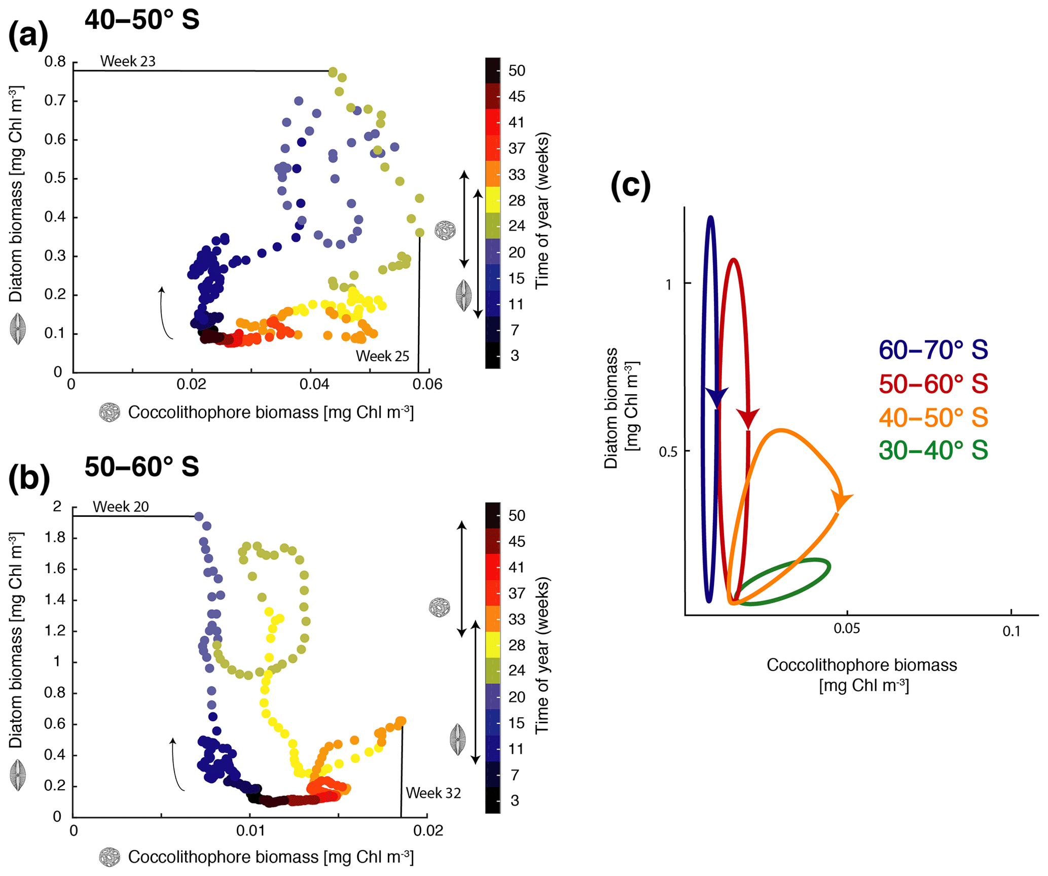
Figure 4Phase diagram of daily surface diatom and coccolithophore chlorophyll biomass (mg Chl m−3) for (a) 40–50∘ S and (b) 50–60∘ S. The colors indicate the time of the year (given in weeks) and the arrow indicates the course of time. Bloom start, bloom end, and bloom duration are marked with arrows on the color bar showing time evolution from July–June for diatoms and coccolithophores, and bloom peak is drawn directly into the phase diagram. (c) Sketch of diatom and coccolithophore chlorophyll biomass evolution (mg Chl m−3) for the different latitudinal bands. Lowest biomass in bottom left; arrows indicate temporal evolution. For details on the definition of the bloom metrics, see the Supplement.
In summary, ROMS–BEC reproduces the spatial patterns of SO phytoplankton biomass and community composition reasonably well. Summer coccolithophore biomass is highest north of 50∘ S, an area coinciding with the observed GCB, where several PFTs coexist in our simulation. In contrast, diatom biomass peaks south of 60∘ S, where they dominate the community (>80 % of total NPP; see Fig. 2a).
4.4 Bloom characteristics and seasonal succession
Generally, with increasing latitude, coccolithophore blooms in ROMS–BEC start and peak later (Fig. 4a and b) and the bloom amplitude decreases (Fig. 4c). Between 40 and 50∘ S, where their maximum in absolute biomass is located (up to 3.9 mmol C m−3; Fig. 1c), coccolithophore blooms in ROMS–BEC start in week 17 (October) and peak in week 25 (December, at about 0.06 mg Chl m−3; Fig. 4a). Peak coccolithophore biomass thereby precedes the maximum contribution of coccolithophores (29 %) to total surface phytoplankton biomass in early February (Fig. 3a). Between 50 and 60∘ S, coccolithophore blooms start in week 29 (January). Coccolithophores contribute up to 10 % to total phytoplankton biomass in late February in our model (Fig. 3b), coinciding with a peak absolute biomass of 0.019 mg Chl m−3 in week 32 (Fig. 4b).
As for coccolithophores, the diatom bloom onset and peak times are later at higher latitudes (Fig. 4a and b). However, in contrast to coccolithophore blooms, the diatom bloom peak increases with latitude (Fig. 4c). Diatom blooms start in week 9 (August) and peak in weeks 23 and 20 (November, at 0.8 and 2.3 mg Chl m−3) between 40–50 and 50–60∘ S, respectively (Fig. 4a and b). Thereby, diatom blooms precede coccolithophore blooms in ROMS–BEC. In our model, diatoms dominate total phytoplankton biomass everywhere south of 40∘ S (Fig. 2a) and diatoms therefore dominate total chlorophyll bloom dynamics. Overall, the timing of the coccolithophore blooms agrees well with observations, but blooms of diatoms tend to start and peak too early and at too-high chlorophyll concentrations in ROMS–BEC when compared to satellite estimates (especially south of 60∘ S; not shown). More specifically, PIC imagery (a proxy for coccolithophore abundance) suggests annual peak concentrations in December and January for 40–50 and 50–60∘ S (NASA-OBPG, 2014c), comparing well with the simulated peaks in December and February. Soppa et al. (2016) find diatom biomass to peak around mid-December (40–60∘ S) and between mid-January and mid-February south of 60∘ S, about 1–2 months later than in our simulation. Additionally, while the simulated peak diatom chlorophyll biomass is close to the value suggested by Soppa et al. (2016) for 40–60∘ S (0.4 vs. 0.25 mg Chl m−3), the simulated peak diatom chlorophyll biomass is 6-fold higher south of 60∘ S (not shown).
Despite these discrepancies, the simulated succession pattern of diatoms and coccolithophores agrees with that suggested for the GCB. In situ studies for the GCB area have inferred the succession of diatoms by coccolithophores from depleted silicic acid levels coinciding with high coccolithophore abundance between 40 and 65∘ S, especially for the Patagonian Shelf (Balch et al., 2014, 2016; Painter et al., 2010), supporting the seasonal dynamics simulated by ROMS–BEC. In the following sections, we assess the controlling factors of the simulated spatial and temporal variability, with a particular focus on the biogeography of coccolithophores and their interplay with diatoms. For this, we restrict the discussion to the latitudinal bands between 40–50 and 50–60∘ S, where coccolithophore biomass is highest (see Sect. 4.3).
4.5 Bottom-up controls on coccolithophore biogeography
Phytoplankton growth rates in BEC are determined as a function of the maximum growth rate and surrounding environmental conditions with respect to temperature, nutrient, and light levels (Eq. 3). Here, we use the relative growth ratio of diatoms versus coccolithophores as defined in Eq. (4) (Hashioka et al., 2013) in order to disentangle the effect of individual bottom-up factors on diatom–coccolithophore competition and their relative contribution to total surface phytoplankton biomass.
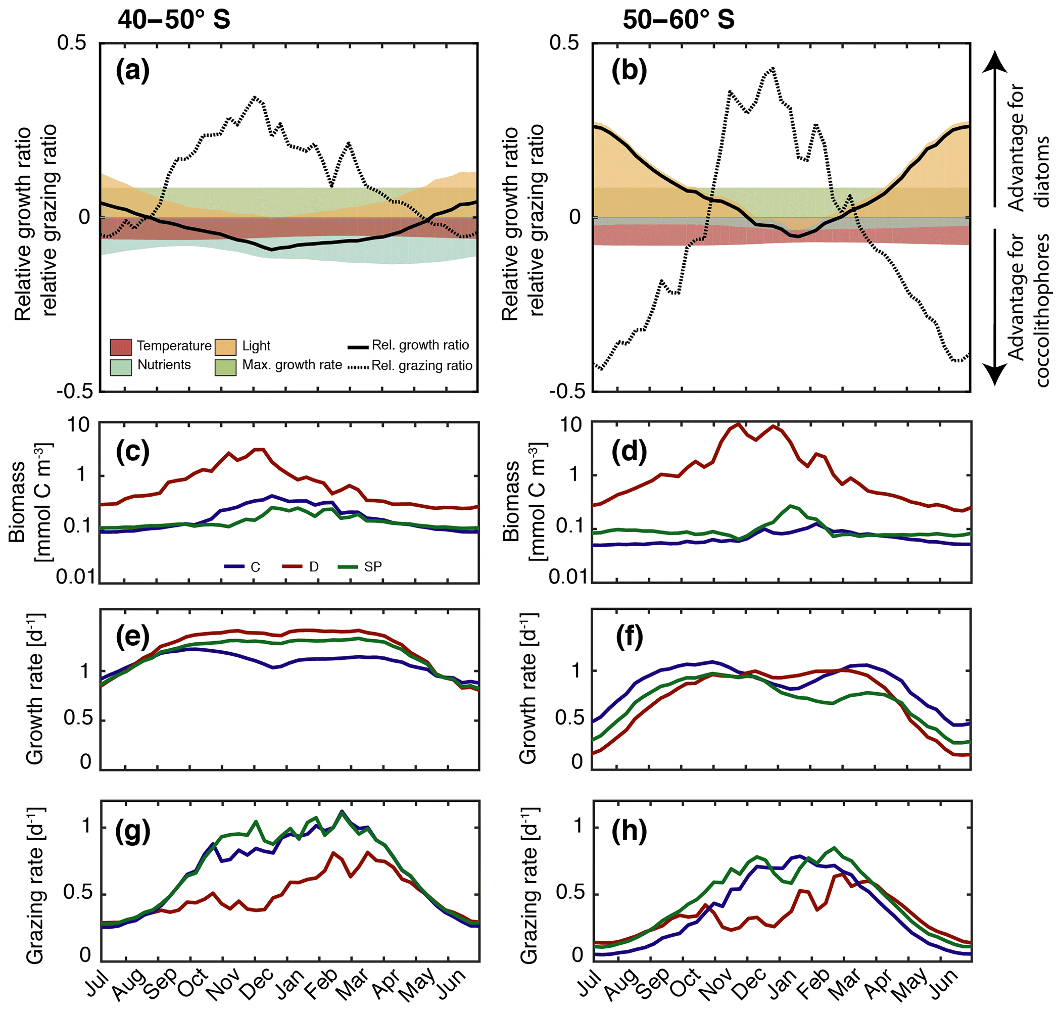
Figure 5(a–b) Relative growth ratio (solid black line) and relative grazing ratio (dashed black line) of diatoms vs. coccolithophores. Colored areas are contributions of the maximum growth rate μmax (green), nutrient limitation (blue), light limitation (yellow), and temperature sensitivity (red) to the relative growth ratio, e.g., the red area represents the term βT of Eq. (4) (see Sect. 3). (c–d) Surface carbon biomass evolution (mmol C m−3), (e–f) specific growth rates (d−1; Eq. 3), and (g–h) biomass-normalized specific grazing rates (d−1, Eq. 6). For (c–h), coccolithophores (C) are shown in blue, diatoms (D) in red, and small phytoplankton (SP) in green. For all metrics, left panels are for 40–50∘ S, and those on the right are for 50–60∘ S.
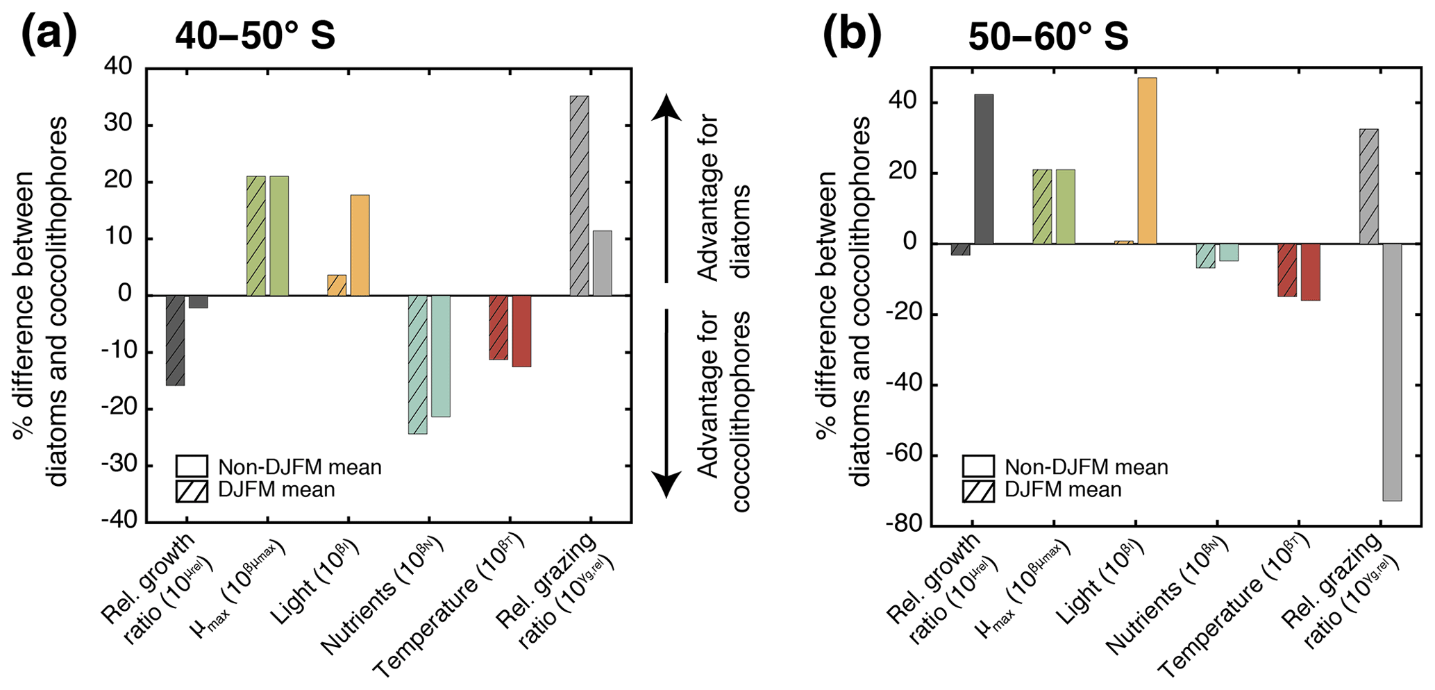
Figure 6Percent difference in growth rate (dark grey), growth-limiting factors (maximum growth rate μmax in green, nutrient limitation in blue, light limitation in yellow, and temperature sensitivity in red), and grazing rate (light grey) of diatoms and coccolithophores for (a) 40–50∘ S and (b) 50–60∘ S. Respective left bar shows the December–March average (DJFM) calculated from the non-log-transformed ratios (e.g., the red bar represents ; see Eq. 4), and the shaded right bars show the average for all other months (non-DJFM). Full seasonal cycle is shown in Fig. 5a and b.
In the latitudinal band between 40 and 50∘ S, the relative growth ratio of diatoms vs. coccolithophores (solid black line in Fig. 5a) is negative from the end of September until the end of April; i.e., the specific growth rate of coccolithophores exceeds that of the diatoms (μCocco>μDiatoms; see Eq. 4). For the four summer months (December–March, DJFM), the specific growth rate of coccolithophores is on average 15 % larger than that of diatoms (Fig. 6a, shaded dark grey bar; calculated from non-log-transformed ratios). This favors the buildup of coccolithophore relative to diatom biomass during this period, partially explaining the comparably high biomass of coccolithophores in this region during summer. This contrasts with the situation in the more southern latitudinal band, i.e., between 50 and 60∘ S, where the relative growth ratio of diatoms vs. coccolithophores (solid black line in Fig. 5b) is negative only for the period between December and mid-February. The growth advantage is also much smaller, amounting to only 3 % during DJFM (Fig. 6b, shaded dark grey bar). This makes it harder for coccolithophores to build up biomass relative to diatoms between 50 and 60∘ S compared to between 40 and 50∘ S.
The relative growth ratio can be separated into the contribution of the maximum growth rate μmax (), temperature (βT), nutrients (βN), and light (βI; see Eq. 4, colored areas in Figs. 5a, b, and 6). The 21 % larger μmax of diatoms compared to that of coccolithophores (Table 1) favors diatom relative to coccolithophore growth all year round in the whole model domain (term in Eq. 4, green area in both Fig. 5a and b is positive). Differences in the temperature limitation of diatoms and coccolithophores arise from differences in Q10 of each PFT (Eq. B5), with coccolithophores being less temperature limited than diatoms (Table 1, term βT in Eq. (4), red area in Fig. 5a is negative). This leads to a DJFM mean growth advantage of 11 % and 15 % of coccolithophores relative to diatoms for 40–50 and 50–60∘ S, respectively (Fig. 6, shaded red bars).
Due to their lower half-saturation constants for nutrient uptake (Table 1), coccolithophores are less nutrient limited than diatoms, resulting in the negative blue areas in Fig. 5a and b (24 % and 7 % less nutrient limited for DJFM between 40–50 and 50–60∘ S, respectively; see Fig. 6, shaded blue bars, and term βN in Eq. 4). For the summer months, amongst all environmental factors, this is the biggest simulated difference between the two latitudinal bands (compare shaded colored bars between Fig. 6a and b). The spatial pattern of the most limiting nutrient for the simulated coccolithophore and diatom growth (Fig. 2b and c, respectively) provides the explanation for this: between 50 and 60∘ S, iron is the most limiting nutrient for both PFTs, but silicic acid is the most limiting nutrient for diatom growth between 40 and 50∘ S. While coccolithophores remain iron limited, silicic acid limitation of diatoms increases the difference in nutrient limitation between coccolithophores and diatoms, thus explaining the greater advantage for coccolithophores between 40 and 50∘ S compared to between 50 and 60∘ S.
In our model, differences in light limitation between coccolithophores and diatoms are controlled by the minor difference in the sensitivity to increases in PAR at low irradiances (αPI) and largely by differences in photoacclimation, i.e., the ability of each PFT to adjust its chlorophyll-to-carbon ratio to surrounding light, nutrient, and temperature conditions (Geider et al., 1998). Coccolithophores have a 9 % lower αPI (Table 1), a generally lower chlorophyll-to-carbon ratio (Fig. S12), and are less nutrient limited than diatoms (blue areas in Fig. 5a and b), resulting in a stronger light limitation of coccolithophores compared to diatoms. While this difference largely disappears in summer (4 % between 40 and 50∘ S and 1 % between 50 and 60∘ S; see Fig. 6, shaded yellow bars, and term βI in Eq. 4), the model simulates pronounced differences between the two latitudinal bands throughout the rest of the year (18 % and 47 %, respectively; see Fig. 6).

Figure 7Relative change in annual mean surface chlorophyll biomass of coccolithophores (C), diatoms (D), and small phytoplankton (SP) for (a) 40–50∘ S and (b) 50–60∘ S for simulations assessing coccolithophore parameter sensitivities (see Table 2). Numbers of relative change are printed if change is larger than ±10 %.
Coccolithophores and diatoms together contribute on average 87 % and 96 % to total DJFM mean surface phytoplankton biomass between 40–50 and 50–60∘ S, respectively (Fig. 3), with diatoms constituting the majority of this biomass. This leaves 13 % and 4 % for small phytoplankton, whose contribution to total biomass levels is thus of the same order of magnitude as that of coccolithophores. SP biomass largely covaries with coccolithophore biomass between 40 and 50∘ S (Fig. 5c), but coccolithophores outcompete SP in summer due to their higher maximum growth rate (Table 1) and growth advantages with respect to temperature, outweighing disadvantages with respect to light and nutrients (Fig. S6a and S7a). Between 50 and 60∘ S, SP biomass is higher than coccolithophore biomass for most of the year (Fig. 5d). Similarly to the diatom–coccolithophore interplay, coccolithophores have a growth advantage relative to SP for a smaller time period (mid-November until April compared to August until mid-May; Fig. S6), while it is slightly bigger in amplitude in summer for this latitudinal band compared to 40–50∘ S (8 % compared to 5 %; Fig. S7b).
In summary, coccolithophores have an advantage in specific growth relative to diatoms in austral summer both between 40 and 50 and between 50 and 60∘ S. Comparing the two latitudinal bands, this advantage is higher for 40–50∘ S, explaining the 10 % greater importance of coccolithophores for total phytoplankton biomass in this band compared to 50–60∘ S (annual mean, Fig. 3). Comparing all environmental factors and the two latitudinal bands, nutrient conditions control the difference in total relative growth ratio between 40–50 and 50–60∘ S in summer, while differences in light limitation drive differences between the summer months and the rest of the year (DJFM vs. non-DJFM; Fig. 6). However, both for 40–50 and 50–60∘ S, despite the higher specific growth rate for part of the year, coccolithophores never outcompete diatoms in terms of absolute biomass (Fig. 5c and d). We calculated whether the length of the growing season is long enough for coccolithophores to outcompete diatoms given their biomass ratio at the end of November, as well as the DJFM growth advantage of 15 % and 3 % (40–50 and 50–60∘ S, respectively; Fig. 6) for coccolithophores, assuming no difference in loss rates between the two PFTs. We found that for 50–60∘ S, the growth advantage of 3 % is not large enough to result in a dominance of coccolithophores over diatoms at the end of the growth season given the 80 times higher diatom biomass at the end of November, in agreement with the simulated biomass evolution (Fig. 5d). For 40–50∘ S, however, our calculations show that despite the 10 times higher biomass of diatoms at the end of November (Fig. 5c), coccolithophores should outcompete diatoms at the end of March given their 15 % higher specific growth rate. But this is valid only if the loss rates are the same for both PFTs. This finding is confirmed by the sensitivity simulation GRAZING, wherein diatoms and coccolithophores experience the same loss rates (see Sect. 4.7), and coccolithophore biomass is indeed larger than that of diatoms between January and March for 40–50∘ S (not shown). Thus, top-down control factors, and zooplankton grazing in particular, are crucial additional factors controlling biomass distribution and its seasonality. In the following, we will assess the importance of grazing by zooplankton in ROMS–BEC for the relative importance of coccolithophores.
4.6 Top-down controls on coccolithophore biogeography
Between 40 and 50∘ S, the simulated relative grazing ratio (Hashioka et al., 2013) of diatoms vs. coccolithophores (dashed black line in Fig. 5a) is positive from mid-September until the end of April; i.e., the coccolithophores experience a stronger grazing pressure (). For the summer months (DJFM), this pressure is, on average, 35 % larger (Fig. 6a, shaded light grey bar), favoring the buildup of diatom relative to coccolithophore biomass. In comparison, between 50 and 60∘ S, the relative grazing ratio of diatoms vs. coccolithophores (dashed black line in Fig. 5b) is positive only from November until the end of March. Further, the grazing disadvantage of coccolithophores is less severe, with coccolithophores experiencing “only” a 23 % larger grazing pressure compared to that of diatoms during DJFM (Fig. 6b, shaded light grey bar).
These differences in the specific grazing rates between coccolithophores and diatoms are of similar magnitude as the differences in the specific growth rates (same scale for solid and dashed lines in Fig. 5a and b). This implies that top-down factors are as important as bottom-up factors in controlling the relative importance of coccolithophores and diatoms. During DJFM, the top-down factors even far outweigh the bottom-up factors in favoring one group over the other; i.e., the differences in the specific grazing rates are 2 (40–50∘ S) and 8 times (50–60∘ S) larger than differences in the specific growth rates (Fig. 6).
The periods when the coccolithophores experience a stronger grazing pressure (positive relative grazing ratios) almost exactly overlap throughout the SO with periods during which they tend to grow faster than the diatoms (negative relative growth ratios; compare solid and dashed black line in Fig. 5a and b). The balance between these two tendencies falls on the grazing side, particularly during summer, resulting in slower biomass accumulation rates for coccolithophores (Fig. 5g and h) and permitting diatoms to take off despite lower growth rates.
In summary, in ROMS–BEC, top-down control by grazing modulates and alters the growth advantages inferred from the bottom-up controls substantially. In fact, top-down controls are even the dominant factor during certain times, making diatoms, because of their lower biomass-normalized grazing rates, overall more successful than coccolithophores in accumulating and sustaining higher biomass concentrations. Thus, at least in our model, the final biomasses and the relative contribution of coccolithophores and diatoms are the product of a complex interplay between the two factors.

Figure 8Sketch summarizing the results from ROMS–BEC: relative importance of coccolithophores (inner circle) and diatoms (outer circle) for total phytoplankton biomass over time in light–silicic acid space for (a) 40∘ S and (b) 60∘ S. Note the different scales for coccolithophores and diatoms. Arrows in the sketch indicate the course of time (white) and the strength of the specific grazing pressure on coccolithophores (blue) and diatoms (green).
4.7 Sensitivity of coccolithophore biogeography to chosen parameter values
We assess the sensitivity of the simulated coccolithophore biogeography by performing a set of sensitivity simulations (runs 1–9 in Table 2). Between 40 and 60∘ S, annual mean surface coccolithophore biomass increases the strongest for GROWTH (2.5-fold and 52 % increase compared to the reference simulation for 40–50 and 50–60∘ S; Fig. 7) and GRAZING (3-fold and 44 % increase). This supports our finding from Sects. 4.5 and 4.6 that top-down and bottom-up controls are equally important in controlling SO coccolithophore biogeography. Coccolithophore biomass decreases by 34 % and 14 % for 40–50∘ S and 50–60∘ S, respectively (with changes <10 % in diatom and >30 % in SP biomass), when making coccolithophore growth more temperature limited (Q10, Fig. 7). With respect to nutrient sensitivities, only the simulation SILICATE leads to significant changes in annual mean coccolithophore biomass for 40–50∘ S (decrease of 55 %, which is compensated for by a doubling in SP biomass). Between 50 and 60∘ S, none of the simulations assessing nutrient sensitivities (runs 5–9) results in significant biomass changes (Fig. 7). This confirms the minor importance of the half-saturation constants for driving the relative importance of diatoms and coccolithophores in this area (blue bars in Fig. 6b). Lastly, coccolithophore biogeography shows little sensitivity to the chosen value of the initial slope of photosynthesis, i.e., αPI. This confirms the result from Sect. 4.5, namely that differences between coccolithophores and diatoms in light limitation are not driven by differences in this parameter (Fig. S5). In summary, we conclude that the simulated coccolithophore biogeography is especially sensitive to the chosen maximum growth and grazing rate (μmax and γmax; Table 1), while it appears insensitive to αPI and all nutrient half-saturation constants, except for the silicic acid limitation of diatoms.
5.1 Biogeochemical implications of SO coccolithophore biogeography
In ROMS–BEC, coccolithophores are a minor but important part of the SO phytoplankton community, contributing 17 % to total annual NPP south of 30∘ S. The model-simulated NPP by SO coccolithophores constitutes about 4.3 %–5.5 % of global NPP (Buitenhuis et al., 2013a). This SO contribution alone is larger than the previously estimated contribution of the global coccolithophore community (<2 %, Jin et al., 2006; 0.4 %, O'Brien, 2015). But this has to be viewed cautiously, since the modeled coccolithophore biomass between 30 and 40∘ S, an area contributing >50 % to coccolithophore production and biomass south of 30∘ S (Table 3), is likely an overestimate (Fig. 1d). At the same time, coccolithophore biomass is underestimated in the model compared to in situ observations south of 40∘ S (Fig. 1d), at least partly balancing the overestimation in the north of the domain. Overall, the scarcity of the in situ data, as well as their high uncertainty of up to 400 % (resulting from the biomass conversion from cell counts; O'Brien et al., 2013), has to be acknowledged, making it difficult to evaluate our model estimate. In addition, simulated coccolithophore biomass and production are prone to uncertainty arising from the chosen parameters, and integrated coccolithophore production south of 30∘ S varies from 2–4.9 Pg C yr−1 (3.1 %–9.6 % of global NPP) in our parameter sensitivity simulations (runs 1–8, except run 6; Table 2). Even while the exact numbers from our modeling studies are uncertain, they are in agreement with previous observational studies from the SO (Charalampopoulou et al., 2016; Hinz et al., 2012; Poulton et al., 2013; Smith et al., 2017), suggesting that the contribution of SO coccolithophores to global NPP is minor.
In contrast, the impact of coccolithophores on global inorganic carbon production (calcification) is much more substantial. Our results suggest that SO coccolithophore calcification contributes ≈24 % to global coccolithophore calcification derived from remote sensing imagery (9.8 %–43.1 % if accounting for uncertainty in the CaCO3 : Corg production ratio of SO Emiliania huxleyi; Krumhardt et al., 2017). Between 40 and 60∘ S (GCB area, area of highest coccolithophore biomass concentrations in both model and observations), the model simulates 8.8 % (3.7 %–16.2 %) of global calcification. This is somewhat lower than the satellite-derived estimate of 18.8 % (15.2 %–22.3 %). But in BEC, we model the rather lightly calcified SO Emiliania huxleyi B ∕ C morphotype (Krumhardt et al., 2017). While Emiliania huxleyi in general, and this morphotype in particular, have been shown to dominate the coccolithophore community in the SO (Balch et al., 2016; Saavedra-Pellitero et al., 2014; Smith et al., 2017), other species such as the more heavily calcified Emiliania huxleyi morphotype A or C. leptoporus might locally contribute overproportionally to total calcification, potentially contributing to the underestimation of modeled calcification. C. leptoporus has been found to locally dominate the coccolithophore community (Saavedra-Pellitero et al., 2014) and has a generally higher CaCO3 : Corg production ratio than Emiliania huxleyi B ∕ C (Krumhardt et al., 2017). Keeping this uncertainty in mind, we can conclude from our simulation that coccolithophores in the GCB are likely at least as important as the surface area they cover (10.9 % of global ocean area, 40–60∘ S), making them an important contributor to the global carbon cycle despite their relatively small contribution to global NPP.
In the context of carbon sequestration, the PIC : POC export ratio is crucial. Our modeled PIC : POC export ratio is higher where and when coccolithophores are important (30–60∘ S, Table 3, especially on the Patagonian Shelf; not shown), in agreement with in situ observations by Balch et al. (2016). A higher PIC : POC export ratio possibly enables more CO2 uptake from the atmosphere due to the ballasting effect of calcite for the downward transport of organic carbon. At the same time, calcification directly increases seawater pCO2, counteracting the ballasting effect. Balch et al. (2016) found that the abundance of coccolithophores in the GCB is high enough to temporarily and locally reverse the sign of the air–sea CO2 flux from a sink to neutral or even a source, inhibiting further CO2 uptake from the atmosphere. The net sign of the combined effect of ballasting and the direct calcification effect on air–sea CO2 exchange remains to be quantified for the GCB as a whole in future research. Nevertheless, the relative importance of coccolithophores in ROMS–BEC implies that it is crucial to estimate potential future change in the relative importance of coccolithophores and/or the CaCO3 : Corg production ratio of coccolithophores for estimating future oceanic carbon cycling in this area in general and oceanic CO2 uptake in particular.
5.2 Succession vs. coexistence: decoupling of maximum specific growth rate and maximum biomass levels by zooplankton grazing in ROMS–BEC
The ROMS–BEC-simulated coccolithophore blooms start and peak later than those of diatoms (Fig. 4), in agreement with the updated version of Margalef's mandala by Balch (2004), predicting the succession of these phytoplankton functional types as a result of changing environmental conditions over time (Margalef, 1978). At the same time, we have seen above that the specific growth rate of coccolithophores in ROMS–BEC is higher than that of diatoms for much of the year (40–50∘ S) and most of austral summer (50–60∘ S; Fig. 5e and f). This implies that not only the spatial coexistence of coccolithophores and diatoms, but also the timing of their peak biomass are the result of interactions between the bottom-up and top-down factors. In fact, phytoplankton specific growth rates are not largest when the respective biomass level is at its maximum in our model (compare Fig. 5c and d with e and f), implying a decoupling in our model between environmental conditions and biomass peaks.
Several metrics have been applied in the past to assess the question of coexistence vs. succession of two phytoplankton PFTs in general or of diatoms and coccolithophores in particular. Traditionally, studies have looked at absolute biomass concentrations only and defined coexistence and succession based on a temporal separation in biomass peaks. For example, Hopkins et al. (2015) defined the succession of diatoms and coccolithophores whenever peaks of total chlorophyll and PIC were more than 16 days apart and identified most of 40–60∘ S as a coexistence area. Instead, Barber and Hiscock (2006) analyzed specific growth rates rather than absolute biomass concentrations. Based on JGOFS data from the equatorial Pacific, their study suggests that all phytoplankton profit equally from improved environmental conditions and that differences the in timing of the biomass peaks can also result simply from differences in the relative abundance at the beginning of the growth season and varying grazing pressures. In agreement with this, Daniels et al. (2015) found coccolithophores to grow simultaneously with an observed diatom bloom in the North Atlantic instead of simply succeeding it.
In agreement with Barber and Hiscock (2006) and Daniels et al. (2015), all phytoplankton respond with an increase in their specific growth rate to improving environmental conditions in spring in ROMS–BEC (Fig. 5e and f), while biomass peaks of, e.g., diatoms and coccolithophores are clearly separated in time because grazing by zooplankton is crucial in controlling biomass evolution in our simulation (see Sect. 4.6). Since maximum specific growth rates, i.e., ideal environmental conditions, do not imply concurrent maximum biomass concentrations in our simulation, the timing of maximum biomass concentrations similarly does not imply ideal growth conditions at that time. This has implications for both in situ and remote-sensing-based studies: typically, in situ studies relate high phytoplankton abundance to local environmental conditions to infer ideal growth conditions. Our results suggest that environmental conditions at the time of maximum abundance do not necessarily represent ideal growth conditions and that a decoupling of specific growth rate and biomass levels as a result of, e.g., top-down controls result in an identification of the succession of phytoplankton types in terms of biomass peaks that is not purely bottom-up driven. Simply comparing peak biomass levels of two PFTs, as is typically done in remote sensing studies assessing phytoplankton seasonality (Hopkins et al., 2015), might similarly result in a misleading picture of ecosystem dynamics and patterns of succession and coexistence. Therefore, assessing remote sensing data with a metric focusing on the relative increase in biomass during the “pre-peak” period rather than just the biomass peak itself might reveal different patterns of coexistence and succession between 40 and 60∘ S, possibly revealing areas of a decoupling between maximum biomass and maximum growth rate. This might reconcile the different metrics and methods used to assess phytoplankton seasonality and give a more comprehensive picture of the interplay of bottom-up and top-down controls.
5.3 Drivers of coccolithophore biogeography
Our model analyses revealed that the absolute biomass concentrations over the course of the year as well as the relative importance of coccolithophores and diatoms are controlled by the spatial and temporal variability in silicic acid and light availability, as well as the higher per biomass grazing pressure on coccolithophores than on diatoms (Fig. 8). A number of in situ studies found an anticorrelation between Emiliania huxleyi abundance in the SO and local silicic acid concentrations (Balch et al., 2014; Hinz et al., 2012; Mohan et al., 2008; Smith et al., 2017). In addition, Balch et al. (2016) found Emiliania huxleyi to be positively correlated with in situ iron levels, concluding that this species occupies the high Fe, low Si niche. This is in agreement with our model results, in which coccolithophores are most important where (40–50∘ S) and when (late austral summer) diatoms become silicic acid limited, but iron levels are still high enough to sustain coccolithophore growth. Temperature has been suggested to be a major driver of latitudinal gradients in SO coccolithophore abundance (Hinz et al., 2012; Saavedra-Pellitero et al., 2014). In our study, differences in temperature sensitivity between diatoms and coccolithophores play a minor role in controlling the relative importance of these two phytoplankton groups (see Figs. 5 and 6). However, globally, the difference in temperature sensitivity (Q10) of diatom and coccolithophore growth appears to be larger (Le Quéré et al., 2016) than what is currently used in ROMS–BEC (1.55 and 1.45, respectively; see Table 1), indicating that we likely underestimate the importance of temperature in controlling the relative importance of diatoms and coccolithophores in our model. In contrast to most other phytoplankton, laboratory experiments have shown coccolithophore growth not to be inhibited at high light levels (Zondervan, 2007), and high light levels have therefore often been considered a prerequisite for elevated coccolithophore abundance (Balch, 2004; Balch et al., 2014; Charalampopoulou et al., 2016; Poulton et al., 2013). In our model, we do not consider the effects of photoinhibition for any of the phytoplankton PFTs. In BEC, differences in summer light levels between 40–50 and 50–60∘ S cannot explain why coccolithophores are relatively more important between 40 and 50 than between 50 and 60∘ S (3 % difference of shaded yellow bar in Fig. 6a and b) and differences in the seasonal amplitude of light levels between the two latitudinal bands appear more important than latitudinal differences in summer alone. If photoinhibitory effects were included in our model, we expect coccolithophores to increase in relative importance in the whole model domain, especially towards the end of the growth season when light levels are highest.
Besides bottom-up factors, we find grazing by zooplankton to be key in explaining the seasonal evolution of the modeled phytoplankton community structure. BEC includes a single zooplankton PFT comprising characteristics of both microzooplankton and macrozooplankton (by assuming microzooplankton feeding on SP and coccolithophores to grow faster than macrozooplankton feeding on diatoms; compare γmax in Table 1; Moore et al., 2002; Sailley et al., 2013), thereby emulating two trophic levels within the zooplankton compartment without explicitly modeling them. However, Sailley et al. (2013) found the coupling between each phytoplankton PFT and the single zooplankton PFT to be strong in BEC, meaning that any increase in phytoplankton biomass leads to a concurrent and immediate increase in zooplankton biomass until saturation is reached. This tight coupling prevents any phytoplankton PFT from escaping grazing pressure and making use of favorable growth conditions, as seen for coccolithophores throughout our analysis domain. Additional explicit zooplankton PFTs and an explicit representation of trophic cascades in the zooplankton compartment might decouple phytoplankton and grazer biomass in both space and time, fostering the importance of coccolithophores relative to diatoms between 40 and 60∘ S and possibly altering total phytoplankton biomass (Le Quéré et al., 2016). The tight coupling between phytoplankton and the single zooplankton in BEC suggests a possible overestimation of the importance of top-down control in controlling the relative importance of coccolithophores in the SO compared to models with more zooplankton complexity.
Besides missing complexity by only including a single zooplankton PFT, the simulated biogeography and controls of the diatom–coccolithophore competition are also sensitive to the chosen zooplankton ingestion function. In ROMS–BEC, we found the effect of both a Holling type III and constraining zooplankton grazing by the total phytoplankton biomass on our results to be similar (runs 12–14 in Table 2): the use of a Holling type III (HOLLING_III) or an active prey-switching (ACTIVE_SWITCHING) grazing formulation, as well as a Holling type II formulation constrained by total phytoplankton biomass (HOLLINGII_SUM_P), instead of our standard Holling type II grazing formulation with fixed prey preferences leads to increased coexistence in the phytoplankton community. This is because either of these changes reduces the grazing pressure on the less abundant PFTs. As a result, coccolithophores and SP increase in relative biomass importance compared to diatoms in all three sensitivity simulations (Fig. S9). At the same time, coccolithophore biomass is pushed outside of the observed range for both sensitivity cases (Fig. S9), indicating a parameter retuning to be necessary for a true comparison of the drivers of coccolithophore biogeography across simulations. Regardless, this again highlights the strong impact of top-down controls on phytoplankton biogeography in ROMS–BEC.
The key role of zooplankton grazing for determining SO phytoplankton biomass (Garcia et al., 2008; Le Quéré et al., 2016; Painter et al., 2010) and community composition (De Baar, 2005; Granéli et al., 1993; Smetacek et al., 2004) has been demonstrated before, but its possible role for SO coccolithophore biogeography has not yet been addressed. Selective grazing by microzooplankton has been found to be important for the development of coccolithophore blooms in other parts of the ocean in observational (North Sea: Holligan et al., 1993, Devon coast: Fileman et al., 2002, northern North Sea: Archer et al., 2001) and modeling studies (Bering Sea Shelf: Merico et al., 2004). However, recent in situ studies addressing controls on coccolithophore biogeography in the SO (Balch et al., 2016; Charalampopoulou et al., 2016; Hinz et al., 2012; Saavedra-Pellitero et al., 2014) have exclusively focused on bottom-up controls by correlating high coccolithophore abundance with concurrent environmental conditions. Based on our findings, future SO in situ studies should consider both bottom-up and top-down factors when assessing coccolithophore biogeography in space and time.
5.4 Limitations and caveats
Our findings may be impacted by several limitations regarding ecosystem complexity, chosen parameterizations and parameters in BEC, model setup and performance, and the analysis framework. Ecosystem models not only vary in the number of zooplankton PFTs, but also in the chosen grazing formulation (Sailley et al., 2013), e.g., in their functional response regarding the ingestion of prey (Holling, 1959) or in the prey preferences of each predator (variable or fixed). It has been shown previously in global models that the choice of the grazing formulation impacts phytoplankton biogeography and diversity (Prowe et al., 2012; Vallina et al., 2014). For ROMS–BEC, the chosen grazing formulation quantitatively impacts our results, but does not qualitatively change the importance of top-down factors. This finding agrees with previous modeling studies, which despite using different ecosystem complexity and grazing formulations came to the conclusion that top-down control is of vital importance for phytoplankton biogeography and diversity (Prowe et al., 2012; Sailley et al., 2013; Vallina et al., 2014). However, we acknowledge the simplicity of the current grazing formulation in BEC, and future research should assess the impact of increased zooplankton complexity on the simulated controls of SO phytoplankton biogeography.
Phytoplankton biogeography is not only affected by choices regarding ecosystem complexity and parameters, but also by biases in the underlying physical and biogeochemical fields. In summary, both the temperature and ML bias have little effect on phytoplankton biogeography, and both phytoplankton community composition and the relative importance of the controls for coccolithophore biogeography change only slightly compared to the reference simulation (runs 10 and 11 in Table 2, Figs. S8 and S9; contribution to total NPP south of 30∘ S: 20 % and 18.7 % SP, 16.7 % and 14.8 % coccolithophores, and 62.3 % and 65.4 % diatoms for TEMP and MLD, respectively, compared to 20.3 %, 16.5 %, and 62.2 % in the reference run). In addition, neither the bias in temperature nor in MLD can explain the overestimation of NPP and total surface chlorophyll at latitudes >60∘ S (not shown). We conclude that biases in the physical fields do not significantly impact our results. However, the positive bias of NPP to total surface chlorophyll remains unexplained in ROMS–BEC at this point. A previous modeling study by Le Quéré et al. (2016) has shown missing complexity in the zooplankton compartment to be a possible explanation for simulated positive phytoplankton biomass biases in the high-latitude SO, and the role of multiple trophic levels needs to be explored in ROMS–BEC.
In this study, we only present results for latitudinal averages even though coccolithophore biomass and its relative importance for total phytoplankton biomass varies across basins (see Fig. 1 and Balch et al., 2016). Additionally, we only address differences in grazing pressure between two phytoplankton PFTs in this study. Aggregation losses and non-grazing mortality (see Eq. 2) contribute <10 % to total phytoplankton loss between 40 and 60∘ S on average (not shown), suggesting them to be of minor importance in controlling the relative importance of coccolithophores and diatoms in this area. While the importance of viral lysis has been shown for the termination of coccolithophore blooms in the North Atlantic (Brussaard, 2004; Evans et al., 2007; Lehahn et al., 2014), to the best of our knowledge, there are only two studies from the SO assessing the relative importance of viral lysis and grazing by zooplankton as sinks for phytoplankton biomass, and both point to a minor importance of viral lysis in this ocean region (Brussaard et al., 2008; Evans and Brussaard, 2012). However, none of these studies explicitly assessed the importance for coccolithophore biomass dynamics, which should be investigated in future observational studies. Ultimately, coccolithophore growth and calcification in BEC are currently not dependent on ambient CO2 concentrations. However, both the study by Trull et al. (2018) and the review by Krumhardt et al. (2017) suggest carbonate chemistry to be of minor importance in controlling the relative importance of coccolithophores in the SO at present, as both specific growth rates and CaCO3 : Corg production ratios of SO coccolithophores appear rather insensitive to variations in ambient CO2 (Krumhardt et al., 2017). Concurrently, the CaCO3 : Corg production ratio has been shown to depend on surrounding temperature, light, and nutrient levels. However, for SO coccolithophores, data are scarce and the resulting functional dependencies remain unclear (Krumhardt et al., 2017). We thus cannot estimate the effect of a varying CaCO3 : Corg production ratio on our results.
This modeling study is the first to comprehensively assess the importance of both bottom-up and top-down factors in controlling the relative importance of coccolithophores and diatoms in the SO over a complete annual cycle. We find that coccolithophores contribute 16.5 % to total annual NPP south of 30∘ S in ROMS–BEC, making them an important member of the SO phytoplankton community. Based on our results, SO coccolithophores alone contribute 5 % to global NPP. We therefore recommend the inclusion of an explicit coccolithophore PFT in global ecosystem models and the development of existing implementations (Gregg and Casey, 2007a; Kvale et al., 2015; Le Quéré et al., 2016) to more adequately simulate both tropical and subpolar coccolithophore populations and to better constrain their contribution to global NPP.
In our model, coccolithophore biomass is higher when diatoms are most limited by silicic acid and when light levels are highest, i.e., north of 50∘ S and towards the end of the growing season. Yet the coccolithophore biomass never gets close to that of the diatoms. This is a consequence of top-down control, i.e., the fact that the coccolithophores are subject to a much larger biomass specific grazing pressure than the diatoms. Consequently, both abiotic and biotic interactions have to be considered over the course of the growing season to assess controls on coccolithophore biogeography, both experimentally and in modeling studies. Top-down factors are important regulators of phytoplankton biomass dynamics not only in the SO, but also globally (Behrenfeld, 2014). Without being restricted to the SO by the regional model setup used here, future work with global models should better quantify regional variability in the relative importance of bottom-up and top-down factors in controlling phytoplankton biogeography.
Coccolithophores impact biogeochemical cycles, especially organic matter cycling, carbon sequestration, and oceanic carbon uptake both via photosynthesis and calcification, leading to cascading effects on the global carbon cycle and hence climate. Thus, it is crucial to more quantitatively assess the contribution of this crucial phytoplankton group to changes in these processes in the past, present, and future ocean.
Model data are available upon email request to the first author (cara.nissen@usys.ethz.ch) or in the ETH library archive (available at https://www.research-collection.ethz.ch/handle/20.500.11850/304530, last access: 19 November 2018; Nissen et al., 2018).
Table A1Data sets used for model evaluation. Please see Sect. S1 for a more detailed description of the data used to evaluate simulated phytoplankton biogeography, community structure, and phenology.
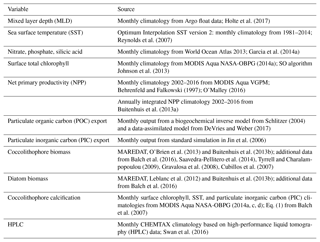
Changes over time in phytoplankton biomass P (mmol C m−3) of phytoplankton i () are controlled by growth and loss terms:
with γg denoting loss by zooplankton grazing, γm loss by non-grazing mortality, and γa loss by aggregation.
B1 Phytoplankton growth
The specific growth rate μi (d−1) of phytoplankton i is determined by the maximum growth rate (see Table 1), which is modified by environmental conditions with respect to temperature (T), nutrients (N), and irradiance (I), following
The temperature function f(T) is an exponential function (see Fig. S10a) of <1 for temperatures below Tref=30 ∘C, modified by the constant Q10 specific to every phytoplankton i (see Table 1) describing the growth rate increase for every temperature increase of 10 ∘C.
Generally, the smaller the Q10, the weaker the temperature limitation of the respective phytoplankton.
The limitation by surrounding nutrients Li(N) is first calculated separately for each nutrient (nitrogen, phosphorus, iron for all phytoplankton, silicic acid for diatoms only) following a Michaelis–Menten function (see Table 1 for half-saturation constants for the respective nutrient and phytoplankton i). For iron (Fe) and silicic acid (SiO3), the limitation factor is calculated following (see Fig. S10c)
For nitrogen and phosphorus, the limitation factor is calculated as the combined limitation by nutrient N and M (nitrate (NO3) and ammonium (NH4) for nitrogen, phosphate (PO4), and dissolved organic phosphorus (DOP) for phosphorus) following
Then, only the most limiting nutrient is used to limit the phytoplankton growth rate:
The light limitation function hi(I) accounts for photoacclimation effects by including the chlorophyll-to-carbon ratio θi, as well as the nutrient and temperature limitation of the respective phytoplankton i (see Fig. S10b).
Generally, the higher the αPI, temperature, and nutrient stress, and the higher the chlorophyll-to-carbon ratio of the respective phytoplankton, the weaker the light limitation.
In ROMS–BEC as used in this study, coccolithophore growth is linearly reduced at temperatures <6 ∘C following
Additionally, coccolithophore growth is set to zero at PAR levels <1 W m−2 (Zondervan, 2007).
Calcification by coccolithophores is proportional to the photosynthetic growth of coccolithophores with a constant CaCO3 : Corg production ratio of 0.2.
Diazotroph growth is zero at temperatures <14 ∘C in BEC, consistent with studies showing diazotroph growth and N2 fixation to be of very minor importance in polar waters (Luo et al., 2012). For consistency within the user community of BEC, we decided to keep diazotrophs as a phytoplankton PFT, even though the imposed temperature threshold makes them a very minor player in the SO phytoplankton community. A sensitivity study in which showed that the results presented in this study are unaffected by the presence of diazotrophs in BEC (not shown).
B2 Phytoplankton loss
In ROMS–BEC, the loss rates of phytoplankton biomass are computed using a corrected phytoplankton biomass to limit phytoplankton loss rates at low biomass.
In this equation, is the threshold of phytoplankton biomass Pi below which no losses occur ( mmol C m−3 and mmol C m−3).
The grazing rate (mmol C m−3 d−1) of the generic zooplankton Z (mmol C m−3) on the respective phytoplankton i (mmol C m−3) is described by (see Fig. S10d)
with
The non-grazing mortality rate (mmol C m−3 d−1) of phytoplankton i (mmol C m−3) is the product of a maximum mortality rate (d−1) scaled by the temperature function fi(T) with the modified phytoplankton biomass :
with being 0.15 d−1 for diazotrophs and 0.12 d−1 for all other phytoplankton.
Aggregation losses are assumed only to occur for diatoms, small phytoplankton, and coccolithophores. The aggregation rate (mmol C m−3 d−1) of phytoplankton i (mmol C m−3) is described by
with being 0.01 d−1 for small phytoplankton and coccolithophores and 0.02 d−1 for diatoms and with being 0.9 d−1 for all three phytoplankton.
The supplement related to this article is available online at: https://doi.org/10.5194/bg-15-6997-2018-supplement.
NG, MV, and CN conceived the study. CN, FAH, and MM set up the model simulations. CN performed the analysis. CN and MV wrote the paper. All authors contributed to the interpretation of the results and to the paper. NG, MV, and MM supervised this study.
The authors declare that they have no conflict of interest.
We would like thank all the scientists who contributed phytoplankton and
zooplankton cell count data to the MAREDAT initiative, as well as
William Balch, Helen Smith, Mariem Saavedra-Pellitero, Gustaaf Hallegraeff,
José-Abel Flores, and Alex Poulton for making additional coccolithophore
or diatom cell count data available for this study. Furthermore, we would
like to thank Martin Frischknecht, Elisa Lovecchio, and Domitille Louchard
for valuable feedback and Damian Loher for technical support. Lastly, we
thank referee no. 1 and Sergio Vallina for their valuable reviews and
comments, which have improved the quality of the paper. This research
was financially supported by the Swiss Federal Institute of Technology
Zürich (ETH Zürich) and the Swiss National Science Foundation
(project SOGate, grant no. 200021_153452). The simulations were performed at
the HPC cluster of ETH Zürich, Euler, which is located in the Swiss
Supercomputing Center (CSCS) in Lugano and operated by ETH ITS Scientific IT
Services in Zürich. Model output is available upon request to the
corresponding author, Cara Nissen (cara.nissen@usys.ethz.ch).
Edited by: Julia Uitz
Reviewed by: Sergio M. Vallina and one anonymous referee
Anderson, L. A. and Sarmiento, J. L.: Redfield ratios of remineralization determined by nutrient data analysis, Global Biogeochem. Cy., 8, 65–80, https://doi.org/10.1029/93GB03318, 1994. a
Archer, S., Widdicombe, C., Tarran, G., Rees, A., and Burkill, P.: Production and turnover of particulate dimethylsulphoniopropionate during a coccolithophore bloom in the northern North Sea, Aquat. Microb. Ecol., 24, 225–241, https://doi.org/10.3354/ame024225, 2001. a
Armstrong, R. A., Lee, C., Hedges, J. I., Honjo, S., and Wakeham, S. G.: A new, mechanistic model for organic carbon fluxes in the ocean based on the quantitative association of POC with ballast minerals, Deep-Sea Res. Pt. II, 49, 219–236, https://doi.org/10.1016/s0967-0645(01)00101-1, 2002. a
Balch, W. M.: Re-evaluation of the physiological ecology of coccolithophores, in: Coccolithophores – From Molecular Processes to Global Impact, edited by: Thierstein, H. R. and Young, J. R., Springer, Berlin, 165–190, 2004. a, b
Balch, W. M., Drapeau, D., Bowler, B., and Booth, E.: Prediction of pelagic calcification rates using satellite measurements, Deep-Sea Res. Pt. II, 54, 478–495, https://doi.org/10.1016/j.dsr2.2006.12.006, 2007. a, b
Balch, W. M., Drapeau, D. T., Bowler, B. C., Lyczskowski, E., Booth, E. S., and Alley, D.: The contribution of coccolithophores to the optical and inorganic carbon budgets during the Southern Ocean Gas Exchange Experiment: New evidence in support of the “Great Calcite Belt” hypothesis, J. Geophys. Res., 116, C00F06, https://doi.org/10.1029/2011JC006941, 2011. a, b
Balch, W. M., Drapeau, D. T., Bowler, B. C., Lyczskowski, E. R., Lubelczyk, L. C., Painter, S. C., and Poulton, A. J.: Surface biological, chemical, and optical properties of the Patagonian Shelf coccolithophore bloom, the brightest waters of the Great Calcite Belt, Limnol. Oceanogr., 59, 1715–1732, https://doi.org/10.4319/lo.2014.59.5.1715, 2014. a, b, c, d, e, f
Balch, W. M., Bates, N. R., Lam, P. J., Twining, B. S., Rosengard, S. Z., Bowler, B. C., Drapeau, D. T., Garley, R., Lubelczyk, L. C., Mitchell, C., and Rauschenberg, S.: Factors regulating the Great Calcite Belt in the Southern Ocean and its biogeochemical significance, Global Biogeochem. Cy., 30, 1199–1214, https://doi.org/10.1002/2016GB005414, 2016. a, b, c, d, e, f, g, h, i, j, k, l, m, n, o, p, q, r
Barber, R. T. and Hiscock, M. R.: A rising tide lifts all phytoplankton: Growth response of other phytoplankton taxa in diatom-dominated blooms, Global Biogeochem. Cy., 20, GB4S03, https://doi.org/10.1029/2006GB002726, 2006. a, b
Beaufort, L., Probert, I., de Garidel-Thoron, T., Bendif, E. M., Ruiz-Pino, D., Metzl, N., Goyet, C., Buchet, N., Coupel, P., Grelaud, M., Rost, B., Rickaby, R., and de Vargas, C.: Sensitivity of coccolithophores to carbonate chemistry and ocean acidification, Nature, 476, 80–83, https://doi.org/10.1038/nature10295, 2011. a
Beaugrand, G., McQuatters-Gollop, A., Edwards, M., and Goberville, E.: Long-term responses of North Atlantic calcifying plankton to climate change, Nat. Clim. Change, 3, 263–267, https://doi.org/10.1038/nclimate1753, 2012. a, b
Behrenfeld, M. J.: Climate-mediated dance of the plankton, Nat. Clim. Change, 4, 880–887, https://doi.org/10.1038/nclimate2349, 2014. a, b
Behrenfeld, M. J. and Falkowski, P. G.: Photosynthetic rates derived from satellite-based chlorophyll concentration, Limnol. Oceanogr., 42, 1–20, https://doi.org/10.4319/lo.1997.42.1.0001, 1997. a
Brussaard, C. P. D.: Viral control of phytoplankton populations - a review, J. Eukaryot. Microbiol., 52, 549–551, https://doi.org/10.1111/j.1550-7408.2005.000vol-cont.x, 2004. a
Brussaard, C. P. D., Timmermans, K. R., Uitz, J., and Veldhuis, M. J. W.: Virioplankton dynamics and virally induced phytoplankton lysis versus microzooplankton grazing southeast of the Kerguelen (Southern Ocean), Deep-Sea Res. Pt. II, 55, 752–765, https://doi.org/10.1016/j.dsr2.2007.12.034, 2008. a
Buitenhuis, E. T., Pangerc, T., Franklin, D. J., Le Quéré, C., and Malin, G.: Growth rates of six coccolithophorid strains as a function of temperature, Limnol. Oceanogr., 53, 1181–1185, https://doi.org/10.4319/lo.2008.53.3.1181, 2008. a, b, c
Buitenhuis, E. T., Hashioka, T., and Le Quéré, C.: Combined constraints on global ocean primary production using observations and models, Global Biogeochem. Cy., 27, 847–858, https://doi.org/10.1002/gbc.20074, 2013a. a, b
Buitenhuis, E. T., Vogt, M., Moriarty, R., Bednaršek, N., Doney, S. C., Leblanc, K., Le Quéré, C., Luo, Y.-W., O'Brien, C., O'Brien, T., Peloquin, J., Schiebel, R., and Swan, C.: MAREDAT: towards a world atlas of MARine Ecosystem DATa, Earth Syst. Sci. Data, 5, 227–239, https://doi.org/10.5194/essd-5-227-2013, 2013b. a, b, c, d, e
Carton, J. A. and Giese, B. S.: A Reanalysis of Ocean Climate Using Simple Ocean Data Assimilation (SODA), Mon. Weather Rev., 136, 2999–3017, https://doi.org/10.1175/2007MWR1978.1, 2008. a
Cermeño, P., Dutkiewicz, S., Harris, R. P., Follows, M., Schofield, O., and Falkowski, P. G.: The role of nutricline depth in regulating the ocean carbon cycle., P. Natl. Acad. Sci. USA, 105, 20344–20349, https://doi.org/10.1073/pnas.0811302106, 2008. a
Charalampopoulou, A., Poulton, A. J., Bakker, D. C. E., Lucas, M. I., Stinchcombe, M. C., and Tyrrell, T.: Environmental drivers of coccolithophore abundance and calcification across Drake Passage (Southern Ocean), Biogeosciences, 13, 5917–5935, https://doi.org/10.5194/bg-13-5917-2016, 2016. a, b, c, d
Cubillos, J. C., Wright, S. W., Nash, G., de Salas, M. F., Griffiths, B., Tilbrook, B., Poisson, A., and Hallegraeff, G. M.: Calcification morphotypes of the coccolithophorid Emiliania huxleyi in the Southern Ocean: changes in 2001 to 2006 compared to historical data, Mar. Ecol. Prog. Ser., 348, 47–54, https://doi.org/10.3354/meps07058, 2007. a, b
Dale, A. W., Nickelsen, L., Scholz, F., Hensen, C., Oschlies, A., and Wallmann, K.: A revised global estimate of dissolved iron fluxes from marine sediments, Global Biogeochem. Cy., 29, 691–707, https://doi.org/10.1002/2014GB005017, 2015. a
Daniels, C. J., Sheward, R. M., and Poulton, A. J.: Biogeochemical implications of comparative growth rates of Emiliania huxleyi and Coccolithus species, Biogeosciences, 11, 6915–6925, https://doi.org/10.5194/bg-11-6915-2014, 2014. a
Daniels, C. J., Poulton, A. J., Esposito, M., Paulsen, M. L., Bellerby, R., St John, M., and Martin, A. P.: Phytoplankton dynamics in contrasting early stage North Atlantic spring blooms: composition, succession, and potential drivers, Biogeosciences, 12, 2395–2409, https://doi.org/10.5194/bg-12-2395-2015, 2015. a, b, c
De Baar, H. J. W.: Synthesis of iron fertilization experiments: From the Iron Age in the Age of Enlightenment, J. Geophys. Res., 110, C09S16, https://doi.org/10.1029/2004JC002601, 2005. a, b
Dee, D. P., Uppala, S. M., Simmons, A. J., Berrisford, P., Poli, P., Kobayashi, S., Andrae, U., Balmaseda, M. A., Balsamo, G., Bauer, P., Bechtold, P., Beljaars, A. C. M., van de Berg, L., Bidlot, J., Bormann, N., Delsol, C., Dragani, R., Fuentes, M., Geer, A. J., Haimberger, L., Healy, S. B., Hersbach, H., Hólm, E. V., Isaksen, L., Kållberg, P., Köhler, M., Matricardi, M., McNally, A. P., Monge-Sanz, B. M., Morcrette, J.-J., Park, B.-K., Peubey, C., de Rosnay, P., Tavolato, C., Thépaut, J.-N., and Vitart, F.: The ERA-Interim reanalysis: configuration and performance of the data assimilation system, Q. J. Roy. Meteor. Soc., 137, 553–597, https://doi.org/10.1002/qj.828, 2011. a
DeVries, T. and Weber, T.: The export and fate of organic matter in the ocean: New constraints from combining satellite and oceanographic tracer observations, Global Biogeochem. Cy., 31, 535–555, https://doi.org/10.1002/2016GB005551, 2017. a
Dutkiewicz, S., Morris, J. J., Follows, M. J., Scott, J., Levitan, O., Dyhrman, S. T., and Berman-Frank, I.: Impact of ocean acidification on the structure of future phytoplankton communities, Nat. Clim. Change, 5, 1002–1006, https://doi.org/10.1038/nclimate2722, 2015. a
Eppley, R. W., Rogers, J. N., and McCarthy, J. J.: Half-saturation constants for uptake of nitrate and ammonium by marine phytoplankton, Limnol. Oceanogr., 14, 912–920, https://doi.org/10.4319/lo.1969.14.6.0912, 1969. a
Evans, C. and Brussaard, C. P. D.: Viral lysis and microzooplankton grazing of phytoplankton throughout the Southern Ocean, Limnol. Oceanogr., 57, 1826–1837, https://doi.org/10.4319/lo.2012.57.6.1826, 2012. a
Evans, C., Kadner, S. V., Darroch, L. J., Wilson, W. H., Liss, P. S., and Malin, G.: The relative significance of viral lysis and microzooplankton grazing as pathways of dimethylsulfoniopropionate (DMSP) cleavage: An Emiliania huxleyi culture study, Limnol. Oceanogr., 52, 1036–1045, https://doi.org/10.4319/lo.2007.52.3.1036, 2007. a
Fileman, E. S., Cummings, D. G., and Llewellyn, C. A.: Microplankton community structure and the impact of microzooplankton grazing during an Emiliania huxleyi bloom, off the Devon coast, J. Mar. Biol. Assoc. UK, 82, 359–368, https://doi.org/10.1017/S0025315402005593, 2002. a
Freeman, N. M. and Lovenduski, N. S.: Decreased calcification in the Southern Ocean over the satellite record, Geophys. Res. Lett., 42, 1834–1840, https://doi.org/10.1002/2014GL062769, 2015. a
Frölicher, T. L., Sarmiento, J. L., Paynter, D. J., Dunne, J. P., Krasting, J. P., and Winton, M.: Dominance of the Southern Ocean in Anthropogenic Carbon and Heat Uptake in CMIP5 Models, J. Climate, 28, 862–886, https://doi.org/10.1175/JCLI-D-14-00117.1, 2015. a
Garcia, H. E., Locarnini, R. A., Boyer, T. P., Antonov, J. I., Baranova, O. K., Zweng, M. M., Reagan, J. R., and Johnson, D. R.: World Ocean Atlas 2013, Volume 4: Dissolved Inorganic Nutrients (phosphate, nitrate, silicate), edited by: Levitus, S., A. Mishonov Technical Ed., NOAA Atlas NESDIS 76, 25 pp., 2014a. a, b
Garcia, H. E., Locarnini, R. A., Boyer, T. P., Antonov, J. I., Baranova, O. K., Zweng, M. M., Reagan, J. R., and Johnson, D. R.: World Ocean Atlas 2013, Volume 3: Dissolved Oxygen, Apparent Oxygen Utilization, and Oxygen Saturation, edited by: Levitus, S., A. Mishonov Technical Ed., NOAA Atlas NESDIS 75, 27 pp., 2014b. a
Garcia, V. M. T., Garcia, C. A. E., Mata, M. M., Pollery, R. C., Piola, A. R., Signorini, S. R., McClain, C. R., and Iglesias-Rodriguez, M. D.: Environmental factors controlling the phytoplankton blooms at the Patagonia shelf-break in spring, Deep-Sea Res. Pt. I, 55, 1150–1166, https://doi.org/10.1016/j.dsr.2008.04.011, 2008. a
Geider, R. J., MacIntyre, H. L., and Kana, T. M.: A dynamic regulatory model of phytoplanktonic acclimation to light, nutrients, and temperature, Limnol. Oceanogr., 43, 679–694, https://doi.org/10.4319/lo.1998.43.4.0679, 1998. a, b
Good, S. A., Martin, M. J., and Rayner, N. A.: EN4: Quality controlled ocean temperature and salinity profiles and monthly objective analyses with uncertainty estimates, J. Geophys. Res.-Oceans, 118, 6704–6716, https://doi.org/10.1002/2013JC009067, 2013. a
Granéli, E., Granéli, W., Rabbani, M. M., Daugbjerg, N., Fransz, G., Roudy, J. C., and Alder, V. A.: The influence of copepod and krill grazing on the species composition of phytoplankton communities from the Scotia Weddell sea, Polar Biol., 13, 201–213, https://doi.org/10.1007/BF00238930, 1993. a, b
Gravalosa, J. M., Flores, J.-A., Sierro, F. J., and Gersonde, R.: Sea surface distribution of coccolithophores in the eastern Pacific sector of the Southern Ocean (Bellingshausen and Amundsen Seas) during the late austral summer of 2001, Mar. Micropaleontol., 69, 16–25, https://doi.org/10.1016/j.marmicro.2007.11.006, 2008. a
Gregg, W. W. and Casey, N. W.: Modeling coccolithophores in the global oceans, Deep-Sea Res. Pt. II, 54, 447–477, https://doi.org/10.1016/j.dsr2.2006.12.007, 2007a. a, b
Gregg, W. W. and Casey, N. W.: Sampling biases in MODIS and SeaWiFS ocean chlorophyll data, Remote Sens. Environ., 111, 25–35, https://doi.org/10.1016/j.rse.2007.03.008, 2007b. a
Hashioka, T., Vogt, M., Yamanaka, Y., Le Quéré, C., Buitenhuis, E. T., Aita, M. N., Alvain, S., Bopp, L., Hirata, T., Lima, I., Sailley, S., and Doney, S. C.: Phytoplankton competition during the spring bloom in four plankton functional type models, Biogeosciences, 10, 6833–6850, https://doi.org/10.5194/bg-10-6833-2013, 2013. a, b, c, d, e, f, g
Haumann, F. A.: Southern Ocean response to recent changes in surface freshwater fluxes, PhD Thesis, ETH Zürich, 2016. a, b, c
Heinle, M.: The effects of light, temperature and nutrients on coccolithophores and implications for biogeochemical models, PhD thesis, University of East Anglia, 2013. a
Hinz, D. J., Poulton, A. J., Nielsdóttir, M. C., Steigenberger, S., Korb, R. E., Achterberg, E. P., and Bibby, T. S.: Comparative seasonal biogeography of mineralising nannoplankton in the Scotia Sea: Emiliania huxleyi, Fragilariopsis spp. and Tetraparma pelagica, Deep-Sea Res. Pt. II, 59–60, 57–66, https://doi.org/10.1016/j.dsr2.2011.09.002, 2012. a, b, c, d, e, f
Holligan, P. M., Fernández, E., Aiken, J., Balch, W. M., Boyd, P., Burkill, P. H., Finch, M., Groom, S. B., Malin, G., Muller, K., Purdie, D. A., Robinson, C., Trees, C. C., Turner, S. M., and van der Wal, P.: A biogeochemical study of the coccolithophore, Emiliania huxleyi, in the North Atlantic, Global Biogeochem. Cy., 7, 879–900, https://doi.org/10.1029/93GB01731, 1993. a
Holling, C. S.: The Components of Predation as Revealed by a Study of Small-Mammal Predation of the European Pine Sawfly, Can. Entomol., 91, 293–320, https://doi.org/10.4039/Ent91293-5, 1959. a, b, c
Holte, J., Talley, L. D., Gilson, J., and Roemmich, D.: An Argo mixed layer climatology and database, Geophys. Res. Lett., 44, 5618–5626, https://doi.org/10.1002/2017GL073426, 2017. a, b
Hopkins, J., Henson, S. A., Painter, S. C., Tyrrell, T., and Poulton, A. J.: Phenological characteristics of global coccolithophore blooms, Global Biogeochem. Cy., 29, 239–253, https://doi.org/10.1002/2014GB004919, 2015. a, b, c, d
Iglesias-Rodríguez, M. D., Armstrong, R., Feely, R., Hood, R., Kleypas, J., Milliman, J. D., Sabine, C., and Sarmiento, J. L.: Progress made in study of ocean's calcium carbonate budget, EOS T. Am. Geophys. Un., 83, 365–375, https://doi.org/10.1029/2002EO000267, 2002. a
Iglesias-Rodríguez, M. D., Halloran, P. R., Rickaby, R. E. M., Hall, I. R., Colmenero-Hidalgo, E., Gittins, J. R., Green, D. R. H., Tyrrell, T., Gibbs, S. J., von Dassow, P., Rehm, E., Armbrust, E. V., and Boessenkool, K. P.: Phytoplankton calcification in a high-CO2 world., Science (New York, N.Y.), 320, 336–340, https://doi.org/10.1126/science.1154122, 2008. a
Jin, X., Gruber, N., Dunne, J. P., Sarmiento, J. L., and Armstrong, R. A.: Diagnosing the contribution of phytoplankton functional groups to the production and export of particulate organic carbon, CaCO3, and opal from global nutrient and alkalinity distributions, Global Biogeochem. Cy., 20, GB2015, https://doi.org/10.1029/2005GB002532, 2006. a, b
Johnson, R., Strutton, P. G., Wright, S. W., McMinn, A., and Meiners, K. M.: Three improved satellite chlorophyll algorithms for the Southern Ocean, J. Geophys. Res.-Oceans, 118, 3694–3703, https://doi.org/10.1002/jgrc.20270, 2013. a, b, c
Krumhardt, K. M., Lovenduski, N. S., Iglesias-Rodriguez, M. D., and Kleypas, J. A.: Coccolithophore growth and calcification in a changing ocean, Prog. Oceanogr., 159, 276–295, https://doi.org/10.1016/j.pocean.2017.10.007, 2017. a, b, c, d, e, f, g, h, i, j
Kvale, K. F., Meissner, K. J., Keller, D. P., Eby, M., and Schmittner, A.: Explicit Planktic Calcifiers in the University of Victoria Earth System Climate Model, Version 2.9, Atmos.-Ocean, 53, 332–350, https://doi.org/10.1080/07055900.2015.1049112, 2015. a
Laufkötter, C., Vogt, M., Gruber, N., Aumont, O., Bopp, L., Doney, S. C., Dunne, J. P., Hauck, J., John, J. G., Lima, I. D., Seferian, R., and Völker, C.: Projected decreases in future marine export production: the role of the carbon flux through the upper ocean ecosystem, Biogeosciences, 13, 4023–4047, https://doi.org/10.5194/bg-13-4023-2016, 2016. a
Lauvset, S. K., Key, R. M., Olsen, A., van Heuven, S., Velo, A., Lin, X., Schirnick, C., Kozyr, A., Tanhua, T., Hoppema, M., Jutterström, S., Steinfeldt, R., Jeansson, E., Ishii, M., Perez, F. F., Suzuki, T., and Watelet, S.: A new global interior ocean mapped climatology: the GLODAP version 2, Earth Syst. Sci. Data, 8, 325–340, https://doi.org/10.5194/essd-8-325-2016, 2016. a
Le Quéré, C., Buitenhuis, E. T., Moriarty, R., Alvain, S., Aumont, O., Bopp, L., Chollet, S., Enright, C., Franklin, D. J., Geider, R. J., Harrison, S. P., Hirst, A. G., Larsen, S., Legendre, L., Platt, T., Prentice, I. C., Rivkin, R. B., Sailley, S., Sathyendranath, S., Stephens, N., Vogt, M., and Vallina, S. M.: Role of zooplankton dynamics for Southern Ocean phytoplankton biomass and global biogeochemical cycles, Biogeosciences, 13, 4111–4133, https://doi.org/10.5194/bg-13-4111-2016, 2016. a, b, c, d, e, f, g, h, i
Leblanc, K., Arístegui, J., Armand, L., Assmy, P., Beker, B., Bode, A., Breton, E., Cornet, V., Gibson, J., Gosselin, M.-P., Kopczynska, E., Marshall, H., Peloquin, J., Piontkovski, S., Poulton, A. J., Quéguiner, B., Schiebel, R., Shipe, R., Stefels, J., van Leeuwe, M. A., Varela, M., Widdicombe, C., and Yallop, M.: A global diatom database – abundance, biovolume and biomass in the world ocean, Earth Syst. Sci. Data, 4, 149–165, https://doi.org/10.5194/essd-4-149-2012, 2012. a, b
Lehahn, Y., Koren, I., Schatz, D., Frada, M., Sheyn, U., Boss, E., Efrati, S., Rudich, Y., Trainic, M., Sharoni, S., Laber, C., DiTullio, G. R., Coolen, M. J. L., Martins, A. M., Van Mooy, B. A. S., Bidle, K. D., and Vardi, A.: Decoupling Physical from Biological Processes to Assess the Impact of Viruses on a Mesoscale Algal Bloom, Curr. Biol., 24, 2041–2046, https://doi.org/10.1016/j.cub.2014.07.046, 2014. a
Letelier, R. M. and Karl, D. M.: Trichodesmium spp. physiology and nutrient fluxes in the North Pacific subtropical gyre, Aquat. Microb. Ecol., 15, 265–276, https://doi.org/10.3354/ame015265, 1998. a
Locarnini, R. A., Mishonov, A. V., Antonov, J. I., Boyer, T. P., Garcia, H. E., Baranova, O. K., Zweng, M. M., Paver, C. R., Reagan, J. R., Johnson, D. R., Hamilton, M., and Seidov, D.: World Ocean Atlas 2013, Volume 1: Temperature, edited by: Levitus, S., Ed., A. Mishonov Technical Ed.; NOAA Atlas NESDIS 73, 40 pp., 2013. a
Luo, Y.-W., Doney, S. C., Anderson, L. A., Benavides, M., Berman-Frank, I., Bode, A., Bonnet, S., Boström, K. H., Böttjer, D., Capone, D. G., Carpenter, E. J., Chen, Y. L., Church, M. J., Dore, J. E., Falcón, L. I., Fernández, A., Foster, R. A., Furuya, K., Gómez, F., Gundersen, K., Hynes, A. M., Karl, D. M., Kitajima, S., Langlois, R. J., LaRoche, J., Letelier, R. M., Marañón, E., McGillicuddy Jr., D. J., Moisander, P. H., Moore, C. M., Mouriño-Carballido, B., Mulholland, M. R., Needoba, J. A., Orcutt, K. M., Poulton, A. J., Rahav, E., Raimbault, P., Rees, A. P., Riemann, L., Shiozaki, T., Subramaniam, A., Tyrrell, T., Turk-Kubo, K. A., Varela, M., Villareal, T. A., Webb, E. A., White, A. E., Wu, J., and Zehr, J. P.: Database of diazotrophs in global ocean: abundance, biomass and nitrogen fixation rates, Earth Syst. Sci. Data, 4, 47–73, https://doi.org/10.5194/essd-4-47-2012, 2012. a
Mahowald, N. M., Engelstaedter, S., Luo, C., Sealy, A., Artaxo, P., Benitez-Nelson, C., Bonnet, S., Chen, Y., Chuang, P. Y., Cohen, D. D., Dulac, F., Herut, B., Johansen, A. M., Kubilay, N., Losno, R., Maenhaut, W., Paytan, A., Prospero, J. M., Shank, L. M., and Siefert, R. L.: Atmospheric Iron Deposition: Global Distribution, Variability, and Human Perturbations, Annu. Rev. Mar. Sci., 1, 245–278, https://doi.org/10.1146/annurev.marine.010908.163727, 2009. a
Margalef, R.: Life-forms of phytoplankton as survival alternatives in an unstable environment, Oceanol. Acta, 1, 493–509, 1978. a, b, c
Merico, A., Tyrrell, T., Lessard, E. J., Oguz, T., Stabeno, P. J., Zeeman, S. I., and Whitledge, T. E.: Modelling phytoplankton succession on the Bering Sea shelf: role of climate influences and trophic interactions in generating Emiliania huxleyi blooms 1997–2000, Deep-Sea Res. Pt. I, 51, 1803–1826, https://doi.org/10.1016/j.dsr.2004.07.003, 2004. a
Mohan, R., Mergulhao, L. P., Guptha, M. V. S., Rajakumar, A., Thamban, M., Anil Kumar, N., Sudhakar, M., and Ravindra, R.: Ecology of coccolithophores in the Indian sector of the Southern Ocean, Mar. Micropaleontol., 67, 30–45, https://doi.org/10.1016/j.marmicro.2007.08.005, 2008. a
Monteiro, F. M., Bach, L. T., Brownlee, C., Bown, P., Rickaby, R. E. M., Poulton, A. J., Tyrrell, T., Beaufort, L., Dutkiewicz, S., Gibbs, S., Gutowska, M. A., Lee, R., Riebesell, U., Young, J., and Ridgwell, A.: Why marine phytoplankton calcify, Science Advances, 2, e1501822, https://doi.org/10.1126/sciadv.1501822, 2016. a
Moore, J. K., Doney, S. C., Kleypas, J. A., Glover, D. M., and Fung, I. Y.: An intermediate complexity marine ecosystem model for the global domain, Deep-Sea Res. Pt. II, 49, 403–462, https://doi.org/10.1016/S0967-0645(01)00108-4, 2002. a, b, c
Moore, J. K., Doney, S. C., and Lindsay, K.: Upper ocean ecosystem dynamics and iron cycling in a global three-dimensional model, Global Biogeochem. Cy., 18, GB4028, https://doi.org/10.1029/2004GB002220, 2004. a
Moore, J. K., Lindsay, K., Doney, S. C., Long, M. C., and Misumi, K.: Marine Ecosystem Dynamics and Biogeochemical Cycling in the Community Earth System Model [CESM1(BGC)]: Comparison of the 1990s with the 2090s under the RCP4.5 and RCP8.5 Scenarios, J. Climate, 26, 9291–9312, https://doi.org/10.1175/JCLI-D-12-00566.1, 2013. a, b
Morel, A. and Berthon, J.-F.: Surface pigments, algal biomass profiles, and potential production of the euphotic layer: Relationships reinvestigated in view of remote-sensing applications, Limnol. Oceanogr., 34, 1545–1562, https://doi.org/10.4319/lo.1989.34.8.1545, 1989. a
Müller, M. N., Trull, T. W., and Hallegraeff, G. M.: Differing responses of three Southern Ocean Emiliania huxleyi ecotypes to changing seawater carbonate chemistry, Mar. Ecol. Prog. Ser., 531, 81–90, https://doi.org/10.3354/meps11309, 2015. a
NASA-OBPG: NASA Goddard Space Flight Center, Ocean Ecology Laboratory, Ocean Biology Processing Group, Moderate-resolution Imaging Spectroradiometer (MODIS) Aqua Chlorophyll Data, https://doi.org/10.5067/AQUA/MODIS/L3M/CHL/2014, 2014a. a, b, c
NASA-OBPG: NASA Goddard Space Flight Center, Ocean Ecology Laboratory, Ocean Biology Processing Group, Sea-viewing Wide Field-of-view Sensor (SeaWiFS) Chlorophyll Data, https://doi.org/10.5067/ORBVIEW-2/SEAWIFS/L3M/CHL/2014, 2014b. a
NASA-OBPG: NASA Goddard Space Flight Center, Ocean Ecology Laboratory, Ocean Biology Processing Group, Moderate-resolution Imaging Spectroradiometer (MODIS) Aqua Particulate Inorganic Carbon Data, https://doi.org/10.5067/AQUA/MODIS/L3M/PIC/2014, 2014c. a, b
NASA-OBPG: NASA Goddard Space Flight Center, Ocean Ecology Laboratory, Ocean Biology Processing Group, Moderate-resolution Imaging Spectroradiometer (MODIS) Aqua Sea Surface Temperature Data, https://doi.org/10.5067/AQUA/MODIS/L3B/SST/2014/, 2014d. a
Nielsen, M. V.: Growth, dark respiration and photosynthetic parameters of the coccolithophorid Emiliania Huxleyi (Prymnesiophyceae) acclimated to different day length-irradiance combinations, J. Phycol., 33, 818–822, https://doi.org/10.1111/j.0022-3646.1997.00818.x, 1997. a
Nissen, C., Vogt, M., Gruber, N., Münnich, M., and Haumann, F. A.: ROMS-BEC model data: Factors controlling coccolithophore biogeography in the Southern Ocean, https://doi.org/10.3929/ethz-b-000304530, 2018. a, b
O'Brien, C. J.: Global-scale distributions of marine haptophyte phytoplankton, PhD Thesis, ETH Zürich, 2015. a
O'Brien, C. J., Peloquin, J. A., Vogt, M., Heinle, M., Gruber, N., Ajani, P., Andruleit, H., Arístegui, J., Beaufort, L., Estrada, M., Karentz, D., Kopczynska, E., Lee, R., Poulton, A. J., Pritchard, T., and Widdicombe, C.: Global marine plankton functional type biomass distributions: coccolithophores, Earth Syst. Sci. Data, 5, 259–276, https://doi.org/10.5194/essd-5-259-2013, 2013. a, b, c, d, e
O'Malley, R.: Ocean Productivity website, available at: http://www.science.oregonstate.edu/ocean.productivity/index.php, last access: 16 May 2016. a
Painter, S. C., Poulton, A. J., Allen, J. T., Pidcock, R., and Balch, W. M.: The COPAS'08 expedition to the Patagonian Shelf: Physical and environmental conditions during the 2008 coccolithophore bloom, Cont. Shelf. Res., 30, 1907–1923, https://doi.org/10.1016/j.csr.2010.08.013, 2010. a, b, c, d
Poulton, A. J., Painter, S. C., Young, J. R., Bates, N. R., Bowler, B., Drapeau, D., Lyczsckowski, E., and Balch, W. M.: The 2008 Emiliania huxleyi bloom along the Patagonian Shelf: Ecology, biogeochemistry, and cellular calcification, Global Biogeochem. Cy., 27, 1023–1033, https://doi.org/10.1002/2013GB004641, 2013. a, b, c
Prowe, A. E. F., Pahlow, M., Dutkiewicz, S., Follows, M., and Oschlies, A.: Top-down control of marine phytoplankton diversity in a global ecosystem model, Prog. Oceanogr., 101, 1–13, https://doi.org/10.1016/j.pocean.2011.11.016, 2012. a, b, c
Reynolds, R. W., Smith, T. M., Liu, C., Chelton, D. B., Casey, K. S., and Schlax, M. G.: Daily High-Resolution-Blended Analyses for Sea Surface Temperature, J. Climate, 20, 5473–5496, https://doi.org/10.1175/2007JCLI1824.1, 2007. a, b
Riebesell, U., Zondervan, I., Rost, B., Tortell, P. D., Zeebe, R. E., and Morel, F. M.: Reduced calcification of marine plankton in response to increased atmospheric CO2, Nature, 407, 364–367, https://doi.org/10.1038/35030078, 2000. a
Rivero-Calle, S., Gnanadesikan, A., Del Castillo, C. E., Balch, W. M., and Guikema, S. D.: Multidecadal increase in North Atlantic coccolithophores and the potential role of rising CO2, Science, 350, 1533–1537, https://doi.org/10.1126/science.aaa8026, 2015. a
Saavedra-Pellitero, M., Baumann, K.-H., Flores, J.-A., and Gersonde, R.: Biogeographic distribution of living coccolithophores in the Pacific sector of the Southern Ocean, Mar. Micropaleontol., 109, 1–20, https://doi.org/10.1016/j.marmicro.2014.03.003, 2014. a, b, c, d, e, f, g, h, i
Sailley, S. F., Vogt, M., Doney, S. C., Aita, M. N., Bopp, L., Buitenhuis, E. T., Hashioka, T., Lima, I., Le Quéré, C., and Yamanaka, Y.: Comparing food web structures and dynamics across a suite of global marine ecosystem models, Ecol. Model., 261–262, 43–57, https://doi.org/10.1016/j.ecolmodel.2013.04.006, 2013. a, b, c, d, e, f
Sarmiento, J. L., Dunne, J., Gnanadesikan, A., Key, R. M., Matsumoto, K., and Slater, R.: A new estimate of the CaCO3 to organic carbon export ratio, Global Biogeochem. Cy., 16, 54-1–54-12, https://doi.org/10.1029/2002GB001919, 2002. a
Sarmiento, J. L., Gruber, N., Brzezinski, M. A., and Dunne, J. P.: High-latitude controls of thermocline nutrients and low latitude biological productivity, Nature, 427, 56–60, https://doi.org/10.1038/nature02127, 2004. a
Sarthou, G., Timmermans, K. R., Blain, S., and Tréguer, P.: Growth physiology and fate of diatoms in the ocean: a review, J. Sea Res., 53, 25–42, https://doi.org/10.1016/j.seares.2004.01.007, 2005. a
Sathyendranath, S., Stuart, V., Nair, A., Oka, K., Nakane, T., Bouman, H., Forget, M. H., Maass, H., and Platt, T.: Carbon-to-chlorophyll ratio and growth rate of phytoplankton in the sea, Mar. Ecol. Prog. Ser., 383, 73–84, https://doi.org/10.3354/meps07998, 2009. a
Schlitzer, R.: Export Production in the Equatorial and North Pacific Derived from Dissolved Oxygen, Nutrient and Carbon Data, J. Oceanogr., 60, 53–62, https://doi.org/10.1023/B:JOCE.0000038318.38916.e6, 2004. a
Schlüter, L., Lohbeck, K. T., Gutowska, M. A., Gröger, J. P., Riebesell, U., and Reusch, T. B. H.: Adaptation of a globally important coccolithophore to ocean warming and acidification, Nat. Clim. Change, 4, 1024–1030, https://doi.org/10.1038/nclimate2379, 2014. a
Shchepetkin, A. F. and McWilliams, J. C.: The regional oceanic modeling system (ROMS): a split-explicit, free-surface, topography-following-coordinate oceanic model, Ocean Model., 9, 347–404, https://doi.org/10.1016/j.ocemod.2004.08.002, 2005. a
Smetacek, V., Assmy, P., and Henjes, J.: The role of grazing in structuring Southern Ocean pelagic ecosystems and biogeochemical cycles, Antarct. Sci., 16, 541–558, https://doi.org/10.1017/S0954102004002317, 2004. a, b
Smith, H. E. K., Poulton, A. J., Garley, R., Hopkins, J., Lubelczyk, L. C., Drapeau, D. T., Rauschenberg, S., Twining, B. S., Bates, N. R., and Balch, W. M.: The influence of environmental variability on the biogeography of coccolithophores and diatoms in the Great Calcite Belt, Biogeosciences, 14, 4905–4925, https://doi.org/10.5194/bg-14-4905-2017, 2017. a, b, c
Soppa, M., Hirata, T., Silva, B., Dinter, T., Peeken, I., Wiegmann, S., and Bracher, A.: Global Retrieval of Diatom Abundance Based on Phytoplankton Pigments and Satellite Data, Remote Sensing, 6, 10089–10106, https://doi.org/10.3390/rs61010089, 2014. a, b, c
Soppa, M., Völker, C., and Bracher, A.: Diatom Phenology in the Southern Ocean: Mean Patterns, Trends and the Role of Climate Oscillations, Remote Sensing, 8, 420, https://doi.org/10.3390/rs8050420, 2016. a, b, c, d
Swan, C. M., Vogt, M., Gruber, N., and Laufkötter, C.: A global seasonal surface ocean climatology of phytoplankton types based on CHEMTAX analysis of HPLC pigments, Deep-Sea Res. Pt. I, 109, 137–156, https://doi.org/10.1016/j.dsr.2015.12.002, 2016. a, b, c, d
Takao, S., Hirawake, T., Hashida, G., Sasaki, H., Hattori, H., and Suzuki, K.: Phytoplankton community composition and photosynthetic physiology in the Australian sector of the Southern Ocean during the austral summer of 2010/2011, Polar Biol., 37, 1563–1578, https://doi.org/10.1007/s00300-014-1542-6, 2014. a, b
Trull, T. W., Passmore, A., Davies, D. M., Smit, T., Berry, K., and Tilbrook, B.: Distribution of planktonic biogenic carbonate organisms in the Southern Ocean south of Australia: a baseline for ocean acidification impact assessment, Biogeosciences, 15, 31–49, https://doi.org/10.5194/bg-15-31-2018, 2018. a, b, c, d
Tyrrell, T. and Charalampopoulou, A.: Coccolithophore size, abundance and calcification across Drake Passage (Southern Ocean), 2009, https://doi.org/10.1594/PANGAEA.771715, 2009. a
Vallina, S., Ward, B., Dutkiewicz, S., and Follows, M.: Maximal feeding with active prey-switching: A kill-the-winner functional response and its effect on global diversity and biogeography, Prog. Oceanogr., 120, 93–109, https://doi.org/10.1016/j.pocean.2013.08.001, 2014. a, b, c, d
Winter, A., Henderiks, J., Beaufort, L., Rickaby, R. E. M., and Brown, C. W.: Poleward expansion of the coccolithophore Emiliania huxleyi, J. Plankton Res., 36, 316–325, https://doi.org/10.1093/plankt/fbt110, 2013. a, b
Wright, S. W., van den Enden, R. L., Pearce, I., Davidson, A. T., Scott, F. J., and Westwood, K. J.: Phytoplankton community structure and stocks in the Southern Ocean (30–80∘ E) determined by CHEMTAX analysis of HPLC pigment signatures, Deep-Sea Res. Pt. II, 57, 758–778, https://doi.org/10.1016/j.dsr2.2009.06.015, 2010. a
Yang, S., Gruber, N., Long, M. C., and Vogt, M.: ENSO-Driven Variability of Denitrification and Suboxia in the Eastern Tropical Pacific Ocean, Global Biogeochem. Cy., 31, 1470–1487, https://doi.org/10.1002/2016GB005596, 2017. a
Zondervan, I.: The effects of light, macronutrients, trace metals and CO2 on the production of calcium carbonate and organic carbon in coccolithophores – A review, Deep-Sea Res. Pt. II, 54, 521–537, https://doi.org/10.1016/j.dsr2.2006.12.004, 2007. a, b, c, d
Zweng, M. M., Reagan, J. R., Antonov, J. I., Mishonov, A. V., Boyer, T. P., Garcia, H. E., Baranova, O. K., Johnson, D. R., Seidov, D., and Bidlle, M. M.: World Ocean Atlas 2013, Volume 2: Salinity, Tech. Rep. 1, 2013. a
- Abstract
- Introduction
- Methods
- Analysis framework: factors controlling phytoplankton growth and loss
- Results
- Discussion
- Conclusions
- Data availability
- Appendix A: Data for model evaluation
- Appendix B: BEC equations: phytoplankton growth and loss
- Author contributions
- Competing interests
- Acknowledgements
- References
- Supplement