the Creative Commons Attribution 4.0 License.
the Creative Commons Attribution 4.0 License.
 | 18 Jun 2018
Reviews and syntheses: Carbonyl sulfide as a multi-scale tracer for carbon and water cycles
Sinikka T. Lennartz
Teresa E. Gimeno
Richard Wehr
Georg Wohlfahrt
Yuting Wang
Linda M. J. Kooijmans
Timothy W. Hilton
Sauveur Belviso
Philippe Peylin
Róisín Commane
Huilin Chen
Ivan Mammarella
Kadmiel Maseyk
Max Berkelhammer
King-Fai Li
Dan Yakir
Andrew Zumkehr
Yoko Katayama
Jérôme Ogée
Felix M. Spielmann
Florian Kitz
Bharat Rastogi
Jürgen Kesselmeier
Julia Marshall
Kukka-Maaria Erkkilä
Lisa Wingate
Laura K. Meredith
Rüdiger Bunk
Thomas Launois
Timo Vesala
Johan A. Schmidt
Cédric G. Fichot
Ulli Seibt
Scott Saleska
Eric S. Saltzman
Stephen A. Montzka
Joseph A. Berry
J. Elliott Campbell
For the past decade, observations of carbonyl sulfide (OCS or COS) have been investigated as a proxy for carbon uptake by plants. OCS is destroyed by enzymes that interact with CO2 during photosynthesis, namely carbonic anhydrase (CA) and RuBisCO, where CA is the more important one. The majority of sources of OCS to the atmosphere are geographically separated from this large plant sink, whereas the sources and sinks of CO2 are co-located in ecosystems. The drawdown of OCS can therefore be related to the uptake of CO2 without the added complication of co-located emissions comparable in magnitude. Here we review the state of our understanding of the global OCS cycle and its applications to ecosystem carbon cycle science. OCS uptake is correlated well to plant carbon uptake, especially at the regional scale. OCS can be used in conjunction with other independent measures of ecosystem function, like solar-induced fluorescence and carbon and water isotope studies. More work needs to be done to generate global coverage for OCS observations and to link this powerful atmospheric tracer to systems where fundamental questions concerning the carbon and water cycle remain.


Carbonyl sulfide (OCS or COS, hereafter OCS) observations have emerged as a tool for understanding terrestrial carbon uptake and plant physiology. Some of the enzymes involved in photosynthesis by leaves also efficiently destroy OCS, so that leaves consume OCS whenever they are assimilating CO2 (Protoschill-Krebs and Kesselmeier, 1992; Schenk et al., 2004; Notni et al., 2007). The two molecules diffuse from the atmosphere to the enzymes along a shared pathway, and the rates of OCS and CO2 uptake tend to be closely related (Seibt et al., 2010). Plants do not produce OCS, and consumption in plant leaves is straightforward to observe. In contrast, CO2 uptake is difficult to measure by itself. At ecosystem, regional, and global scales, large respiratory CO2 fluxes from other plant tissues and other organisms obscure the photosynthetic CO2 signal, i.e., gross primary productivity (GPP). OCS is not a perfect tracer for GPP due to the presence of additional sources/sinks of OCS in ecosystems that complicate this relationship. However, these sources/sinks are generally small, so measurements of OCS concentrations and fluxes can still generate useful estimates of photosynthesis, stomatal conductance, or other leaf parameters at temporal and spatial scales that are difficult to observe.
Several independent groups have examined OCS and CO2 observations and come to similar conclusions about links between the plant uptake processes for the two gases. Goldan et al. (1987) linked OCS plant uptake, FOCS, to uptake of CO2, , specifically referring to GPP. Advancing the global perspective, Chin and Davis (1993) thought FOCS was connected to net primary productivity, which includes respiration terms, and this scaling was used in earlier versions of the OCS budget, e.g., Kettle et al. (2002). Sandoval-Soto et al. (2005) re-introduced GPP as the link to FOCS, using available GPP estimates to improve OCS and sulfur budgets, which were their prime interest. Montzka et al. (2007) first proposed to reverse the perspective in the literature and suggested that OCS might be able to supply constraints on gross CO2 fluxes, with Campbell et al. (2008) directly applying it in this way.
Since then, other applications have been developed, including understanding of terrestrial plant productivity since the last ice age (Campbell et al., 2017a), estimating canopy (Yang et al., 2018) and stomatal conductance and enzyme concentrations on the ecosystem scale (Wehr et al., 2017), assessment of the current generation of continental-scale carbon models (e.g., Hilton et al., 2017), and better tracing of large-scale atmospheric processes like convection and tropospheric–stratospheric mass transfers. Many of these applications rely on the fact that the largest fluxes of atmospheric OCS are geographically separated: most atmospheric OCS is generated in surface oceans and is destroyed by terrestrial plants. In practice, these new applications often call for refining the terms of the global budget of OCS.
An abundance of new observations have been made possible by technological innovation. While OCS is the longest-lived and most plentiful sulfur-containing gas in the atmosphere, its low ambient concentration (∼0.5 ppb) makes measurement challenging. Quantification of OCS in air used to require time-consuming pre-concentration before injection into a gas chromatograph (GC) with a mass spectrometer (MS) or other detector. While extended time series remain scarce, 17 years of observations have been generated by the National Oceanic and Atmospheric Administration (NOAA) Global Monitoring Division air monitoring network (Montzka et al., 2007). A system for measuring flask samples for a range of important low-concentration trace gases was modified slightly in early 2000 to enable reliable measurements for OCS. These observations allowed for the first robust evidence of OCS as a tracer for terrestrial CO2 uptake on continental to global scales (Campbell et al., 2008). In 2009, a quantum cascade laser instrument was developed, followed by many improvements in precision and measurement frequency (Stimler et al., 2010a). Current instruments can measure OCS with <0.010 ppb precision and a frequency of 10 Hz (Kooijmans et al., 2016). On larger spatial scales, many Fourier transform infrared spectroscopy (FTIR) stations and three satellites have recently been used to retrieve spectral signals for OCS in the atmosphere.
This review seeks to synthesize our collective understanding of atmospheric OCS, highlight the new questions that these data help answer, and identify the outstanding knowledge gaps to address moving forward. First, we present what information is known from surface-level studies. Then we develop a scaled-up global OCS budget that suggests where there are considerable uncertainties in the flux of OCS to the atmosphere. We examine how the existing data have been applied to estimating GPP and other ecosystem variables. Finally, we describe where data are available and prioritize topics for further research.
The sulfur cycle is arguably the most perturbed element cycle on Earth. Half of sulfur inputs to the atmosphere come from anthropogenic activity (Rice et al., 1981). OCS is the most abundant and longest-lived sulfur-containing gas. Ambient concentrations of OCS are relatively stable over month-long timescales. Observations from flask (Montzka et al., 2007), FTIR (Toon et al., 2018), and Fourier transform spectroscopy (FTS) measurements (Kremser et al., 2015) suggest a small (<5 %) increasing trend in tropospheric OCS for the most recent decade. Over millennia, concentrations may reflect large-scale changes in global plant cover (Aydin et al., 2016; Campbell et al., 2017a).
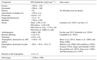
Upscaling ecosystem estimates (Sandoval-Soto et al., 2005) with global transport models are incompatible with atmospheric measurements (Berry et al., 2013; Suntharalingam et al., 2008), suggesting that there may be a large missing source of OCS, sometimes attributed to the tropical oceans; however, individual observations from ocean vessels do not necessarily support this hypothesis (Lennartz et al., 2017). The small increase of OCS in the atmosphere is at least 2 orders of magnitude too small to account for the missing source. Anthropogenic emissions are an important OCS source to the atmosphere, but data for the relevant global industries are incomplete (Zumkehr et al., 2018). Here we analyze our current understanding of global surface–atmosphere OCS exchange and generate new global flux estimates from the bottom up, with no attempt at balancing the atmospheric budget (Fig. 1). We use the convention that positive flux represents emission to the atmosphere and negative flux represents removal.
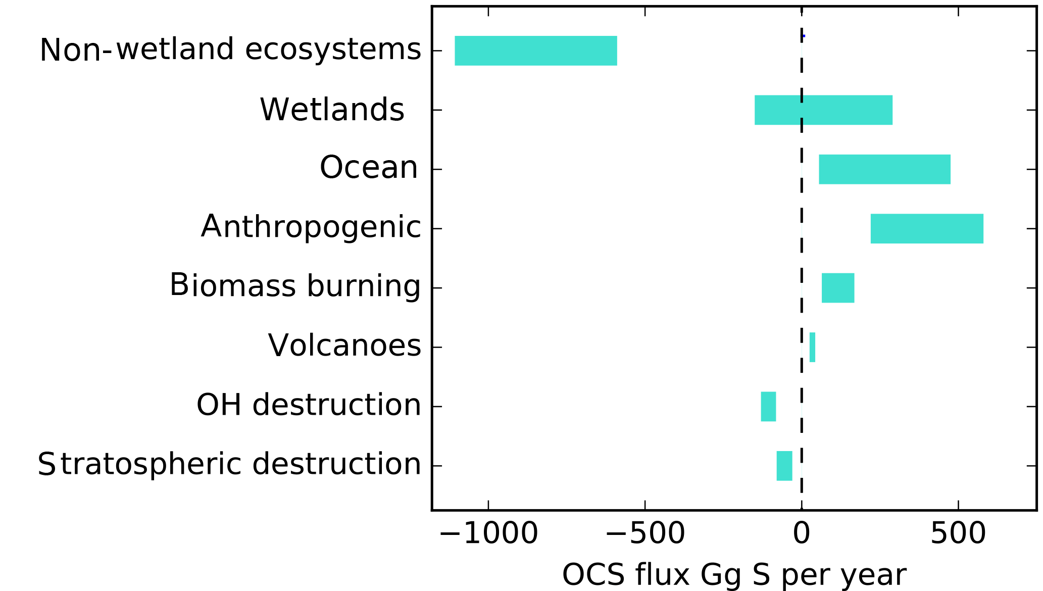
Figure 1A bottom-up budget of atmospheric OCS on the global scale. Positive values indicate a source to the atmosphere. No attempt has been made to preserve mass balance. The contribution of lakes and non-vascular plants is included in the non-wetland ecosystem estimate. The small increase of OCS in the atmosphere is not included in this plot.
2.1 Global atmosphere
OCS in the atmosphere is primarily generated from ocean and anthropogenic sources. A portion of these sources are indirect, emitted as CS2 which can be oxidized to OCS (Zeng et al., 2016). Within the atmosphere, major sinks of OCS are OH oxidation in the troposphere and photolysis in the stratosphere. Besides large volcanic eruptions, OCS is a significant source of sulfur to the stratosphere and was briefly entertained as a geoengineering approach to promote global dimming (Crutzen, 2006). However, the global warming potential of OCS roughly balances whatever global cooling effect it might have (Brühl et al., 2012). Abiotic hydrolysis in the atmosphere plays a small role: while snow and rain were observed to be supersaturated with OCS (Belviso et al., 1989; Mu et al., 2004), even in the densest supersaturated clouds the OCS in the air would represent 99.99 % of the OCS present (Campbell et al., 2017b). Multiple lines of evidence support uptake by plants as the dominant removal mechanism of atmospheric OCS (e.g., Asaf et al., 2013; Berry et al., 2013; Billesbach et al., 2014; Campbell et al., 2008; Glatthor et al., 2017; Hilton et al., 2017; Launois et al., 2015b; Mihalopoulos et al., 1989; Montkza et al., 2007; Protoschill-Krebs and Kesselemeier, 1992; Sandoval-Soto et al., 2005; Stimler, 2010b; Suntharalingham et al., 2008).
The observed atmospheric OCS distribution suggests that seasonality is driven by terrestrial uptake in the Northern Hemisphere and oceanic fluxes in the Southern Hemisphere (Montzka et al., 2007). Improvements in the OCS budget were derived through inverse modeling of NOAA tower and airborne observations on a global scale (Berry et al., 2013; Launois et al., 2015b; Suntharalingam et al., 2008). Lower concentrations were generally found in the terrestrial atmospheric boundary layer compared to the free troposphere during the growing season, and amplitudes of seasonal variability were enhanced at low-altitude stations, particularly those situated mid-continent.
Total column measurements of OCS from ground-based FTS show trends in OCS concentrations coincident with the rise and fall of global rayon production, which creates OCS indirectly (Campbell et al., 2015). Kremser et al. (2015) found an overall positive tropospheric rise of 0.43–0.73 % yr−1 at three sites in the Southern Hemisphere from 2001 to 2014. The trend was interrupted by a sharply decreasing interval from 2008 to 2010, also observed in the global surface flask measurements (Fig. S2; Campbell et al., 2017a). A similar but smaller dip was observed in the stratosphere, indicating that the trends are driven by processes within the troposphere. Over Jungfraujoch, Switzerland, Lejeune et al. (2017) observed a decrease in tropospheric OCS from 1995 to 2002 and an increase from 2002 to 2008; after 2008 no significant trend was observed. An increase in OCS concentrations from the mid-20th-century with a decline around the 1980s was also recorded in firn air (Montzka et al., 2004), following historic rayon production trends.
Changes in terrestrial OCS uptake and possibly the ocean OCS source can be observed from the 54 000-year record from ice cores. Global OCS concentrations dropped 45 to 50 % between the Last Glacial Maximum and the start of the Holocene (Aydin et al., 2016). By the late Holocene, concentrations had risen, and the highest levels were recorded in the 1980s (Campbell et al., 2017a).
Recommendations. Modern seasonal and annual variability of OCS can be validated with smaller vertical profile datasets, e.g., Kato et al. (2011), and data from flights, e.g., Wofsy et al. (2011). Interhemispheric variability on millennia timescales requires ice core data from the Northern Hemisphere: all current ice core data are from the Antarctic (Aydin et al., 2016).
2.2 Terrestrial ecosystems
OCS uptake by terrestrial vegetation is governed mechanistically by the series of diffusive conductances of OCS into the leaf and the reaction rate coefficient for OCS destruction by carbonic anhydrase (CA) (Wohlfahrt et al., 2012), though it can also be destroyed by other photosynthetic enzymes, e.g., RuBisCo (Lorimer and Pierce, 1989). CA is present both in plant leaves and soils, although soil uptake tends to be proportionally much lower than plant uptake. In soil systems, OCS uptake provides information about CA activities within diverse microbial communities. OCS uptake over plants integrates information about the sequential components of the diffusive conductance (the leaf boundary layer, stomatal, and mesophyll conductances) and about CA activity, all important aspects of plant and ecosystem function. Stomatal conductance in particular is a prominent research focus in its own right, as it couples the carbon and water cycles via transpiration and photosynthesis.
Terrestrial plant OCS uptake has typically been derived by scaling estimates of the plant CO2 uptake with proportionality coefficients, such as the empirically derived leaf relative uptake rate ratio (LRU; Sandoval-Soto et al., 2005):
where FOCS is the uptake of OCS into plant leaves; is CO2 uptake; [OCS] and [CO2] are the ambient concentrations of OCS and CO2; and LRU is the ratio of the OCS to CO2 uptake, which is a function of plant type and water and light conditions. The concept of the LRU is a simplification of the leaf CO2 and OCS uptake process. The -to-FOCS relationship depends on the leaf conductance to each gas as it changes with the difference between concentrations inside and outside of the leaf. This requires further modeling to anticipate within-leaf concentrations of OCS and CO2, which cannot be observed directly. To keep the simplicity of the approach, especially when using OCS to evaluate models with many other built-in assumptions, the data-based LRU approximation is sufficient in many cases. We have compiled LRU data (n=53) from an earlier review and merged them with more recent published studies (Berkelhammer et al., 2014; Stimler et al., 2010b, 2011, 2012). The LRUs compiled in Sandoval-Soto et al. (2005) were partly re-calculated in Seibt et al. (2010) to account for the lower gas concentrations in the sample cuvettes. For C3 plants, OCS uptake behavior is attributed to CA activity (Yonemura et al., 2005). As shown in Fig. 2, LRU estimates for C3 species under well-illuminated conditions are positively skewed, with 95 % of the data between 0.7 to 6.2, which coincides with the theoretically expected range of 0.6 to 4.3 (Wohlfahrt et al., 2012). The median, 1.68, is quite close to values reported and used in earlier studies and provides a solid “anchor ratio” for linking C3 plant OCS uptake and photosynthesis in high light. LRU data are fewer for C4 species (n=4), converging to a median of 1.21, reflecting more efficient CO2 uptake rates compared to C3 species (Stimler et al., 2011).
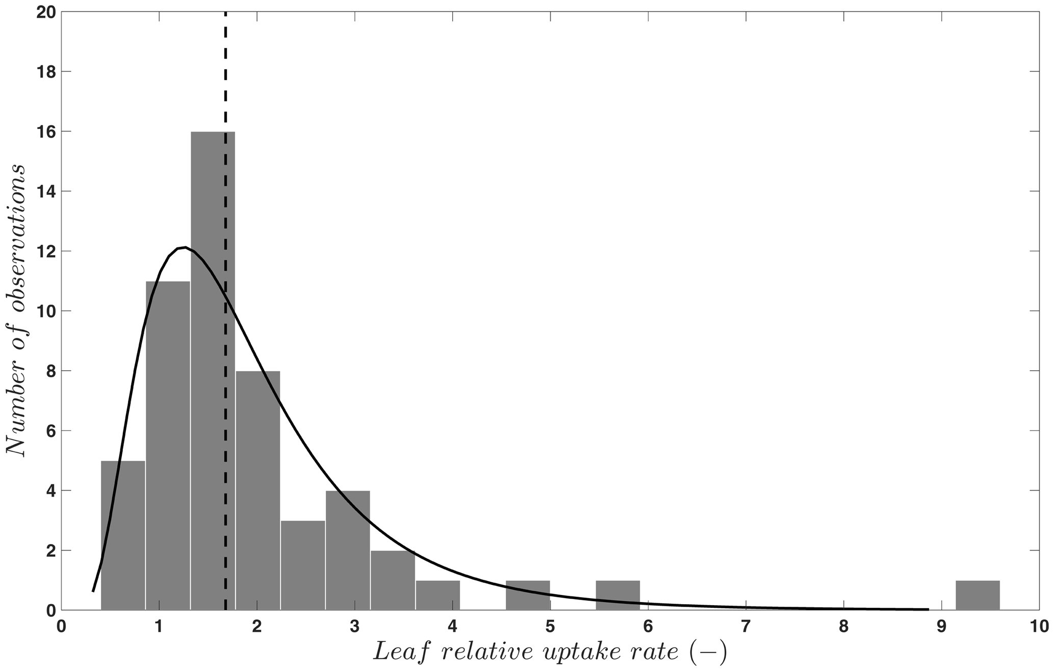
Figure 2Frequency distribution (bars) and a lognormal fit (solid line) to published values (n=53) of the leaf relative uptake rate of C3 species. The vertical line indicates the median (1.68). Published data are from Berkelhammer et al. (2014), Sandoval-Soto et al. (2005), Seibt et al. (2010), and Stimler et al. (2010b, 2011, 2012).
LRU remains fairly constant with changes in boundary layer and stomatal conductance but is expected to deviate due to changes in internal OCS conductance and CA activity (Seibt et al., 2010; Wohlfahrt et al., 2012). The primary environmental driver of LRU is light, and an increase in LRU with decreasing photosynthetically active radiation has been observed at both the leaf (Stimler et al., 2010b, 2011) and ecosystem scale (Maseyk et al., 2014; Commane et al., 2015; Wehr et al., 2017; Yang et al., 2018). This behavior arises because photosynthetic CO2 assimilation is reduced in low light, whereas OCS uptake continues since the reaction with CA is not light dependent (Stimler et al., 2011). Note that since low light reduces CO2 uptake, the flux-weighted effect of the variations in LRU on estimating (or GPP) is also reduced on daily or longer timescales (Yang et al., 2018).
An additional complication is introduced by soil and non-vascular plant processes that both emit and consume OCS, with a few studies reporting net OCS emission under certain conditions comparable in magnitude to net uptake rates during peak growth. Generally, soil OCS fluxes are low compared to plant uptake with a few exceptions (Fig. 3). In non-vascular plants, OCS uptake continues in the dark even when photosynthesis ceases (Gries et al., 1994; Kuhn et al., 1999; Kuhn and Kesselmeier, 2000; Gimeno et al., 2017; Rastogi et al., 2018). Unlike other plants, bryophytes and lichens lack responsive stomata and protective cuticles to control water losses. OCS emissions from these organisms seem to be primarily driven by temperature (Gimeno et al., 2017).
The yearly average land OCS flux rate in recent modeling studies of global budgets (i.e., plant and soil uptake minus soil emissions) ranges from −2.5 to −12.9 (Fig. 3). The only study reporting year-round OCS flux measurements is from a mixed temperate forest, which was a sink for OCS with a net flux of −4.7 during the observation period (Commane et al., 2015). Daily average OCS fluxes during the peak growing season are available from a larger selection of studies and cover the range from −8 to −23 , excluding that of Xu et al. (2002), which found a surprisingly high uptake (–97±11.7 ) from the relaxed eddy accumulation method (Fig. 3). Despite the limited temporal and spatial coverage, these data suggest that some of the larger global land net sink estimates may be too high (Launois et al., 2015b).
The following subsections explore a few aspects of ecosystem OCS exchange in greater detail. Observations and conclusions about forests, grasslands, wetlands, and freshwater ecosystems are explored. Then we examine OCS interactions reported for components of ecosystems: soils, microbial communities, and abiotic hydrolysis and sorption.
Recommendations. Available observations are limited in time and do not cover tropical ecosystems, which contribute almost 60 % of global GPP (Beer et al., 2010). More year-round measurements from a larger number of biomes, in particular those presently underrepresented, are required to provide reliable bottom-up estimates of the total net land OCS flux. The causes for the observed variability in Fig. 2 require more investigation because they hamper the specification of defensible plant-functional-type-specific LRUs (Sandoval-Soto et al., 2005) and the development of models with non-constant LRU (Wohlfahrt et al., 2012). Relatively little is known regarding using OCS to estimate CA activity (Wehr et al., 2017), which is a promising new avenue of OCS research. Within this context, plant physiological and enzymatic adaptations to increasing CO2 and their effects on the exchange of OCS are of special interest.
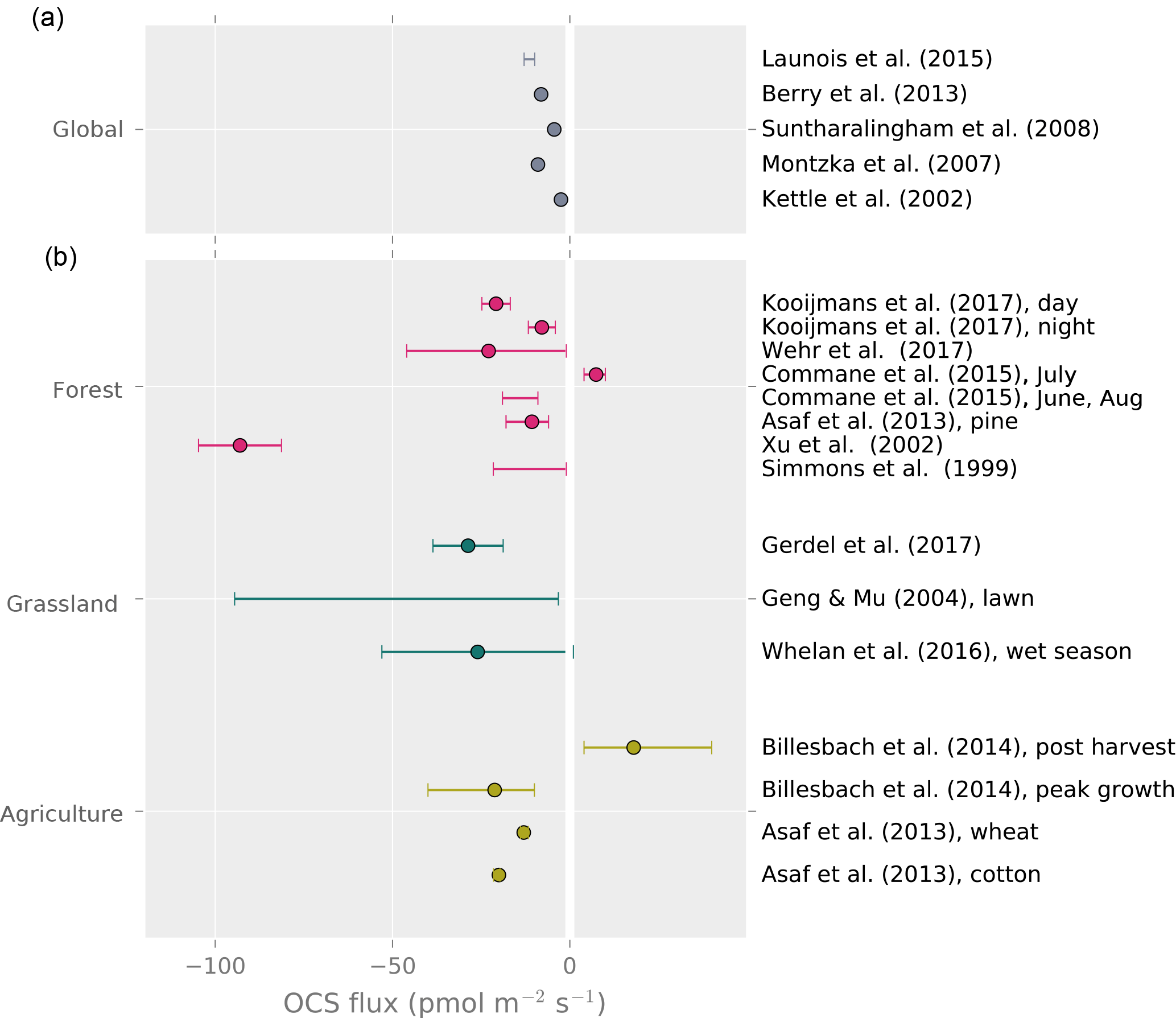
Figure 3Top panel: global average land OCS uptake from modeling studies. Bottom panel: reported averages and ranges of whole-ecosystem, site-level OCS observations. Points represent reported averages; error bars show the uncertainty around the average or the range of observed fluxes where no meaningful average was reported.
2.2.1 Forests
OCS has the potential to overcome many difficulties in studying the carbon balance of forest ecosystems. To partition carbon fluxes, respiration is often quantified at night, when photosynthesis has ceased and turbulent airflow is reduced (Reichstein et al., 2005). This method has systematic uncertainties; e.g., less respiration happens during the day than at night (Wehr et al., 2016). Partitioning with OCS is based on daytime data and does not rely on modeling respiration with limited nighttime flux measurements.
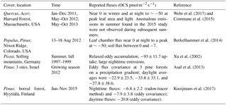
Forests are daytime net sinks for atmospheric OCS, when photosynthesis is occurring in the canopy (Table 1). While the relative uptake of OCS to CO2 by leaves appears stable in high-light conditions, the ratio changes in low light when the net CO2 uptake is reduced (Stimler et al., 2011; Wehr et al., 2017; Rastogi et al., 2018). Forest soil interaction with OCS has been found to be small with respect to leaf uptake (Fig. 3) and straightforward to correct (Belviso et al., 2016; Wehr et al., 2017). Sun et al. (2016) noted that litter was the most important component of soil OCS fluxes in an oak woodland. Otherwise, forest ecosystem OCS uptake appears to be dominated by tree leaves, both during the day and at night (Kooijmans et al., 2017).
Table 1In situ fluxes of forest ecosystems. Some of these data are plotted in Fig. 2.
Recommendations. Tropical forest OCS fluxes would be informative for global OCS modeling efforts and are currently absent from the literature. The OCS tracer approach is particularly useful in high-humidity or foggy environments like the tropics, where traditional estimates of carbon uptake variables via water vapor exchange are ineffective. Additionally, OCS observing towers upstream and downstream of large forested areas could resolve the synoptic-scale variability in forest carbon uptake (Campbell et al., 2017b).
2.2.2 Grasslands
OCS observations can address the need for additional studies on primary productivity in grassland ecosystems. Grasslands generally are considered to behave as carbon sinks or be carbon-neutral but appear highly sensitive to drought and heat waves and can rapidly shift from neutrality to a carbon source (Hoover and Rogers, 2016). Currently OCS grassland studies are scarce (Fig. 3) but indicate a significant role for soils. Theoretical deposition velocities for grasses of 0.75 mm s−1 were reported by Kuhn et al. (1999), and LRU values of 2.0 were reported by Seibt et al. (2010). Whelan and Rhew (2016) made chamber-based estimates of ecosystem fluxes from a California grassland with a distinct growing and non-growing season. Total ecosystem fluxes averaged −26 during the wet season and −6.1 during the dry season. During the wet season, simulated rainfall increased the sink strength. Light and dark flux estimates yielded similar sinks, suggesting either a large role for soils in the ecosystem flux or the presence of open stomata under dark conditions. Yi and Wang (2011) undertook chamber measurements over a grass lawn in subtropical China. Ecosystem fluxes of −19.2 were observed. They noted average soil fluxes of −9.9 that were occasionally greater than 50 % of the total ecosystem flux. The large contribution of soils to the grassland OCS flux was attributed to atmospheric water stress on the plants that led to significant stomatal closure and reduced midday uptake by vegetation. More recently, Gerdel et al. (2017) reported daily average ecosystem-scale OCS fluxes of for a productive managed temperate grassland.
Solar radiation has been identified recently as a controlling factor of grassland soil OCS emissions. Kitz et al. (2017) highlighted that, in grasslands, primary production is devoted to belowground biomass early in the growing season, leading to a situation where exposed soils may be emitting photo-produced OCS simultaneously with high GPP. If unaccounted for, this would lead to an underestimation of the plant component of the total ecosystem OCS flux (Kitz et al., 2017; Whelan and Rhew, 2016).
Recommendations. Grassland plants tend to include mixtures of C3 and C4 species with a relative abundance and importance to GPP evolving over the season. These different photosynthetic pathways are known to exhibit different LRU values. On the one hand, this poses a challenge to direct estimations of GPP from OCS; on the other hand, observations may provide a unique opportunity to study C3 and C4 contributions to GPP. Another pressing research question is the effect of the changing leaf area index of grasses on radiation and related soil emissions.
2.2.3 Wetlands and peatlands
Much of the early work on OCS terrestrial–atmospheric fluxes was conducted in wetlands, perhaps because of the large emissions observed there. Unfortunately, many of these first surveys were conducted with sulfur-free sweep air, significantly biasing the observed net OCS flux compared with that under ambient conditions (Castro and Galloway, 1991).
OCS fluxes have been measured in a variety of wetland ecosystems, including peat bogs, coastal salt marshes, tidal flats, mangrove swamps, and freshwater marshes. Observed ecosystem emission rates vary by 2 orders of magnitude and generally increase with salinity (Fig. 4). OCS emissions in salt marshes usually range from 10 to 300 (Aneja et al., 1981; DeLaune et al., 2002; Li et al., 2016; Steudler and Peterson, 1984, 1985; Whelan et al., 2013), whereas freshwater marshes and bogs have mean emission rates below 10 (DeLaune et al., 2002; Fried et al., 1993) or act as net sinks due to plant uptake (Fried et al., 1993; Liu and Li, 2008; de Mello and Hines, 1994).

Figure 4A summary figure for wetland OCS emissions. Lines indicate minimum to maximum ranges. Studies denoted “S” indicated a soil-only observation, and “S + V” denotes a soil and vegetation observation. Points show reported averages, and error bars show either reported uncertainty or the full range of observations. Note that some earlier observations using sulfur-free air as chamber sweep air have been excluded due to overestimation (Castro and Galloway, 1991).
Although plants are generally OCS sinks, wetland plants may appear as OCS sources. Emergent stems can act as conduits transmitting OCS produced in the soil to the atmosphere, or OCS may be a by-product of processes related to osmotic management by plants in saline environments. For example, in a Batis maritima coastal marsh, vegetated plots were found to have up to 4 times more OCS emission than soil-only plots (Whelan et al., 2013). Growing season OCS emissions may greatly exceed those in the non-growing season (Li et al., 2016), but whether this is caused by environmental factors like temperature and soil saturation or by the developmental stage of plants is unclear.
Recommendations. Assessing the role of plants in the wetland OCS budget would require careful investigation of OCS transport via plant stems and OCS producing capacity of aboveground plant materials and the rhizosphere. More work needs to be done on the evolution of OCS in soils with low redox potential. Additional experiments should aim to help scale up wetland OCS fluxes.
2.2.4 Lakes and rivers
The role of lakes and rivers in the global OCS budget is not well known. OCS production and consumption have been studied in ocean waters, and these processes most likely occur similarly in freshwater. In the ocean, OCS is produced photochemically from chromophoric dissolved organic matter (CDOM) (Ferek and Andreae, 1984) and by a light-independent production that has been linked to sulfur radical formation (Flöck et al., 1997; Zhang et al., 1998). A mechanism for OCS photoproduction was recently described for lake water (Du et al., 2017). Dissolved OCS (Fig. 5) is consumed by abiotic hydrolysis at a rate determined by pH, salinity, and temperature (Fig. 6; Elliott et al., 1989).
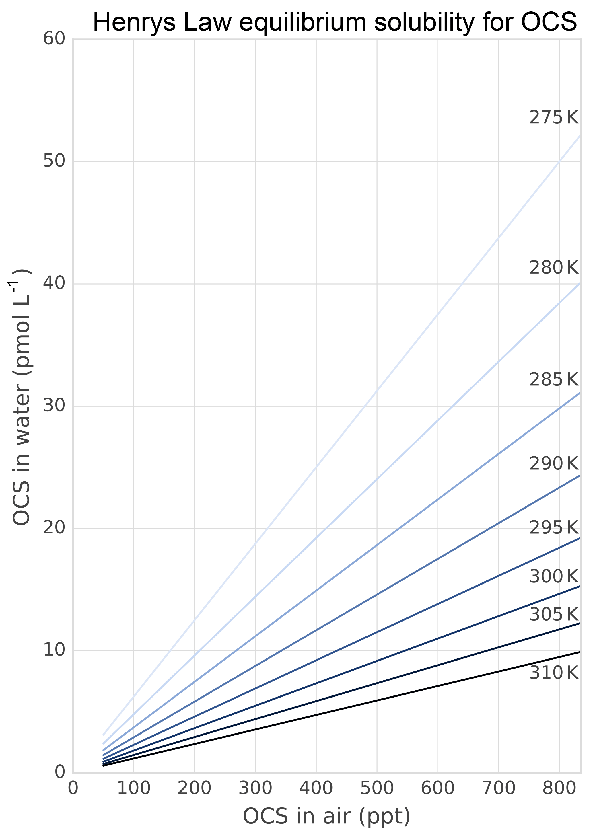
Figure 5Solubility of OCS in water dependent on ambient OCS concentration and temperature as calculated in Sun et al. (2015).
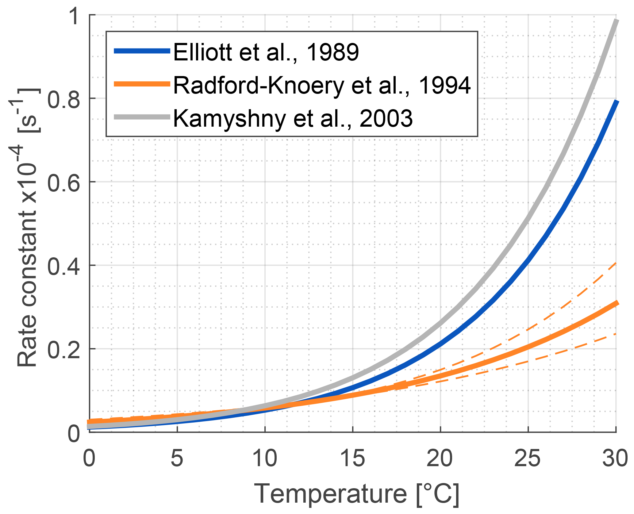
Figure 6Comparison of published hydrolysis rates for OCS based on laboratory experiments with artificial water (Elliott et al., 1989; Kamyshny et al., 2003), and under oceanographic conditions using filtered seawater (Radford-Knȩry et al., 1994). The graph is replotted using equations from original papers at a pH of 8.2.
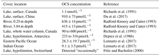
OCS is present in freshwaters at much higher concentrations than those found in the ocean (Table 2). This might be due to more efficient mixing in the ocean surface waters compared to lakes. However, Richards et al. (1991) found that the concentration remained the same throughout the water column and observed a midsummer OCS concentration minimum in 8 of the 11 studied lakes. This latter point was surprising because photochemical production should be highest during the summer months. It has been demonstrated that ocean algae take up OCS, which might explain the low concentrations when light levels are high; however, Blezinger et al. (2000) concluded that the consumption term should be small compared to abiotic hydrolysis and photoproduction.
Table 2OCS concentrations observed in rivers and lakes compared to ocean observations in Lennartz et al. (2017).
To our knowledge, there have not yet been any studies on OCS fluxes using direct flux measurement methods over freshwaters. Richards et al. (1991) calculated OCS fluxes from different lakes in Ontario, Canada, based on concentration measurements and wind-speed-dependent gas transfer coefficients, resulting in fluxes of 2–5 pmol OCS . In another study, Richards et al. (1994) found fluxes of 2–34 pmol OCS in salty lakes. These fluxes are 5 to 75 times higher than those measured in the oceans (Lennartz et al., 2017). There is also an indirect atmospheric OCS source from carbon disulfide (CS2) production (Richards et al., 1991, 1994; Wang et al., 2001), for which little data exist.
Recommendations. Measurements in lakes are easier than in the open ocean while generating more information on the processes that may drive OCS production in both regions. Flux data by eddy covariance (EC) and floating chamber methods from lakes and rivers are suggested. Concurrent measurements should target understanding of the biotic and abiotic factors driving water–air exchange of OCS to provide the basis for upscaling aquatic OCS fluxes, including CS2 concentrations.
2.3 Other terrestrial OCS flux components
2.3.1 Soils
Measurements show that non-wetland soils are predominantly a sink for OCS, and wetland (anoxic) soils are typically a source of OCS. OCS production has also been observed in most non-desert oxic soils when dry, with particularly large emissions from agricultural soil (Fig. 7).

Figure 7Field observations of soil OCS fluxes. Points are reported averages. Error bars are the reported range or the uncertainty of the average. Kuhn et al. (1999) represents an upper range due to under-pressurized soil chambers.
In the field, reported oxic soil OCS fluxes range from near zero up to −10 , with average uptake rates typically between 0 and −5 . Higher uptake fluxes of −10 to −20 have been observed in a grassland soil (Whelan and Rhew, 2016), wheat field soils (Kanda et al., 1995; Maseyk et al., 2014), unplanted rice paddies (Yi et al., 2008), and bare lawn soil (Yi and Wang, 2011). However, under warm and dry conditions, fluxes approached zero in grasslands (Berkelhammer et al., 2014; Whelan and Rhew, 2016) and an oak woodland (Sun et al., 2016). The highest reported uptake rates are nearly −40 , following simulated rainfall in a grassland (Whelan and Rhew, 2016). Sun et al. (2016) also reported a rapid response to re-wetting following a rainstorm in a dry Mediterranean woodland.
Variations in soil OCS fluxes measured in the field have been linked to temperature, soil water content, nutrient status, and CO2 fluxes. Uptake rates have been found to increase with temperature (White et al., 2010; Yi et al., 2008) but also decrease with temperature such that OCS fluxes approached zero or shifted to emissions at temperatures around 15–20 ∘C (Maseyk et al., 2014; Steinbacher et al., 2004; Whelan and Rhew, 2016; Yang et al., 2018). It can be difficult to separate the effects of temperature and soil water content in the field, and seasonal decreases in OCS fluxes may also be associated with lower soil water content (Steinbacher et al., 2004; Sun et al., 2016). Uptake rates have also been found to be stimulated by nutrient addition in the form of fertilizer or lime (Melillo and Steudler, 1989; Simmons, 1999).
Several field studies have found that OCS uptake is positively correlated with rates of soil respiration, or CO2 production (Yi et al., 2007), but these relationships also vary with temperature (Sun et al., 2016, 2017), soil water content (Maseyk et al., 2014), or high-CO2 conditions (Bunk et al., 2017). The relationship with respiration is attributed to the role of microbial activity in OCS consumption, and similar covariance has been seen between OCS and H2 uptake (Belviso et al., 2013), a microbially driven process. Berkelhammer et al. (2014) and Sun et al. (2017) have found that the OCS / CO2 flux ratio has a nonlinear relationship with temperature, such that the ratio decreases (becomes more negative) at lower temperatures but is constant at higher temperatures. Kesselmeier and Hubert (2002) observed both OCS uptake and emission by beech leaf litter that was related to microbial respiration rates. Sun et al. (2016) determined that most of the soil OCS uptake in an oak woodland occurred in the litter layer, composing up to 90 % of the small surface sink.
Extensive laboratory studies demonstrate that OCS uptake is mainly governed by biological activity and physical constraints. Kesselmeier et al. (1999), van Diest and Kesselmeier (2008), and Whelan et al. (2016) characterized the response of several controlling variables such as atmospheric OCS mixing ratios, temperature, and soil water content or water-filled pore space. Clear temperature and soil water content optima are observed for OCS consumption. These optima vary with soil type but indicate water limitation at low soil water content and diffusion resistance at high soil water content. Additionally, other organism-mediated or abiotic processes in the soil, such as photo- or thermal degradation of soil organic matter (Whelan and Rhew, 2015), can play an important role.
The strong activity of sulfate reduction metabolism in anoxic environments is thought to drive OCS production in anoxic wetland soils (see Fig. 4) (Aneja et al., 1981; Kanda et al., 1992; Whelan et al., 2013; Yi et al., 2008). Temperature probably drives the observed seasonal variation of OCS production, with higher fluxes in the summer than winter (Whelan et al., 2013). How much OCS escapes to the atmosphere depends on transport in the soil column. Tidal flooding may inhibit OCS emission from wetland soils due to decreasing gas diffusivity with increasing soil saturation rather than changes in OCS production rates (Whelan et al., 2013).
With high light or temperatures, OCS production in oxic soils can exceed rates found in wetlands. Substantial OCS production has been observed in agricultural fields under both wet and dry conditions (Kitz et al., 2017; Maseyk et al., 2014). OCS fluxes of up to +30 and +60 were related strongly to temperature (Maseyk et al., 2014) and radiation (Kitz et al., 2017), respectively. While most ecosystems do not experience these conditions, almost all soils produce OCS abiotically when air-dried and incubated in the laboratory (Whelan et al., 2016; Liu et al., 2010; Kaisermann et al., 2018; Meredith et al., 2018a). Whelan and Rhew (2015) compared sterilized and living soil samples from the agricultural study site originally investigated in Maseyk et al. (2014), finding that all samples emitted considerable amounts of OCS under high ambient temperature and radiation, with even higher emissions after sterilization. Net OCS emissions can occur from agricultural soils at all water contents (Bunk et al., 2017) develop in summer (Yang et al., 2018), and OCS production rates do not differ significantly in moist and dry soils (Kaisermann et al., 2018). Meredith et al. (2018a) found that OCS soil production rates are higher in low-pH, high-N soils that have relatively greater levels of microbial biosynthesis of S-containing amino acids and concentrations of related S compounds.
Two mechanistic models for soil OCS exchange have been developed and can simulate observed features of soil OCS exchange, such as the responses of OCS uptake to soil water content, temperature, and the transition from OCS sink to source at high soil temperature (Ogée et al., 2016; Sun et al., 2015).
Both models resolve the vertical transport and the source and sink terms of OCS in soil layers. OCS uptake is represented with the Michaelis–Menten enzyme kinetics, dependent on the OCS concentration in each soil layer, whereas OCS production is assumed to follow an exponential relationship with soil temperature, consistent with field observations (Maseyk et al., 2014). Although diffusion across soil layers neither produces nor consumes OCS, altering the OCS concentration profile affects the concentration-dependent uptake of OCS.
Recommendations. Additional experiments are required to understand OCS production in oxic soils. The mechanism of soil production and why some soils are more prone to high production rates is unknown. In wetlands, the interaction between OCS production and transport processes remains poorly understood. If OCS produced by microbes accumulates in isolated soil pore spaces during inundation, subsequent ventilation can lead to an abrupt release, which may appear as high variability in surface emissions. Field experiments using simple transport manipulation (e.g., straight tubes inserted into sediment) interpreted with soil modeling would clarify matters.
2.3.2 Microbial communities
The mechanism of OCS consumption in ecosystems is thought to be mediated by CA, a fairly ubiquitous enzyme present within cyanobacteria, micro-algae, bacteria, and fungi. Purified from soil environments or from culture collections, bacteria and fungi show degradation of OCS at atmospheric concentrations. Mycobacterium spp. purified from soil and Dietzia maris NBRC15801T and Streptomyces ambofaciens NBRC12836T showed significant OCS degradation (Kato et al., 2008; Ogawa et al., 2016). Purified saprotrophic fungi Fusarium solani and Trichoderma spp. were found to decrease atmospheric OCS (Li et al., 2010; Masaki et al., 2016). Some free-living saprophyte Sordariomycetes fungi and Actinomycetales bacteria, dominant in many soils, are also capable of degrading OCS (Harman et al., 2004; Nacke et al., 2011). Sterilized soil inoculated with Mycobacterium spp. showed the ability to take up OCS (Kato et al., 2008). In addition, cell-free extract of Acidianus spp. showed significant catalyzed destruction of OCS (Smeulders et al., 2011). During OCS degradation, soil bacteria introduce isotopic fractionation (Kamezaki et al., 2016; Ogawa et al., 2017). Using different approaches, Bunk et al. (2017), Sauze et al. (2017), and Meredith et al. (2018b) showed that fungi might be the dominant player in soil OCS uptake.
In addition, there exist hyperdiverse microbial communities that colonize the surface of plant leaves or the “phyllosphere” (Vacher et al., 2016). The phyllosphere is an extremely large habitat (estimated in 1 billion km2) hosting microbial population densities ranging from 105 to 107 cells cm−2 of leaf surface (Vorholt, 2012). With respect to OCS, it has already been shown that plant–fungal interactions can cause OCS emissions (Bloem et al., 2012). It is undetermined if these epiphytic microbes are capable of consuming and emitting OCS.
Biotic OCS production is a possibility: in bacteria, novel enzymatic pathways have been described that degrade thiocyanate and isothiocyanate and render OCS as a byproduct (Bezsudnova et al., 2007; Hussain et al., 2013; Katayama et al., 1992; Welte et al., 2016). Evidence for OCS emissions following SCN− degradation has been observed from a range of environmental samples from aquatic and terrestrial origins, indicating a wide distribution of OCS-emitting microorganisms in nature (Yamasaki et al., 2002). Hydrolysis of isothiocyanate, another breakdown product of glucosinolates (Hanschen et al., 2014), by the SaxA protein also yields OCS, as shown in phytopathogenic Pectobacterium sp. (Welte et al., 2016). Some Actinomycetales bacteria and Mucoromycotina fungi, both commonly found in soils, are also known to emit OCS, but the origin and pathway remains unspecified (Masaki et al., 2016; Ogawa et al., 2016).
Recommendations. Further studies should test the connection between the microorganisms that degrade OCS and the candidate enzymes that we assume are performing the degradation. In addition, the magnitude of biotic OCS production in soils is unknown. While sterilized soils exhibit higher OCS production than live soils (Whelan and Rhew, 2015), we have not determined if biotic production is universally insignificant in bulk soils.
2.3.3 Surface sorption and abiotic hydrolysis
Several abiotic processes can affect surface fluxes of OCS. OCS can be hydrolyzed in water and adsorb and desorb on solid surfaces. Abiotic hydrolysis of OCS in water occurs slowly relative to the timescales of typical flux observations (Fig. 6). This is in contrast to the reaction in plant leaves, which is also technically a hydrolysis reaction but is catalyzed by CA. The temperature dependence of OCS solubility was modeled and described by Eq. (20) in Sun et al. (2015): for a OCS concentration in air of 500 ppt, in equilibrium at ambient temperatures, the OCS dissolved in water will be less than 0.5 pmol OCS / mol−1 H2O (Fig. 5). Some portion of the dissolved OCS is destroyed by hydrolysis, following data generated by Elliott et al. (1989). For the rate-limiting step of hydrolysis in near-room-temperature water, the pseudo-first-order rate constant is around s−1. The hydrolysis of OCS gains significance over hours, especially in ice cores (Aydin et al., 2014, 2016).
Under typical environmental conditions, OCS adsorption and desorption is near steady state. OCS adsorbs onto various mineral surfaces at ambient temperatures and can be desorbed at higher temperatures (Devai and DeLaune, 1997). In some ecosystems with large temperature swings, temperature-regulated sorption cannot be ruled out as playing a small role in the variability of observed fluxes.
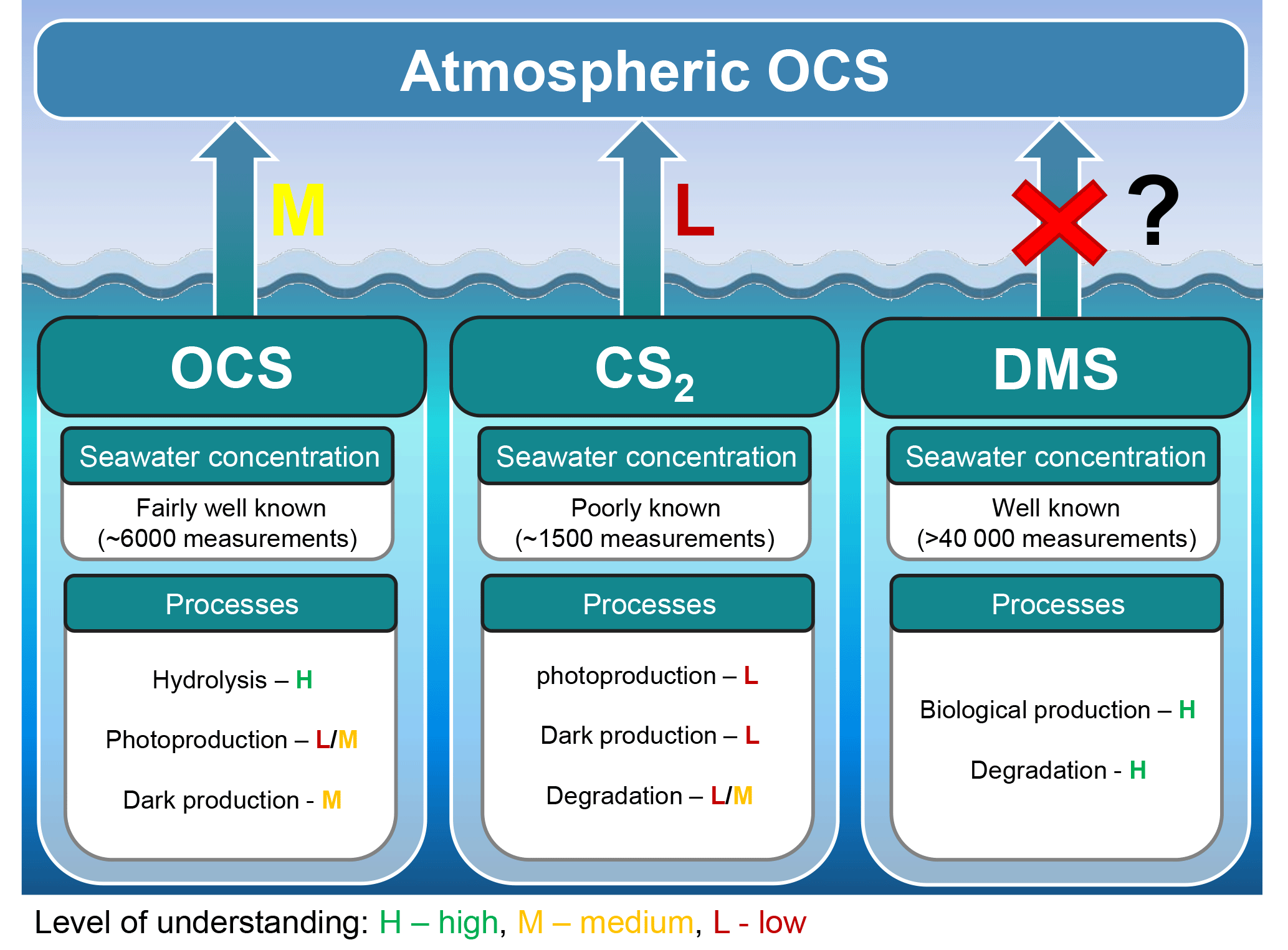
Figure 8Marine contribution to the atmospheric OCS loading from direct and indirect (CS2) emissions. The sea surface concentration determines the magnitude of the oceanic emissions, and the uncertainty in global emissions decreases with increasing numbers of measurements. The understanding of processes is important to extrapolate from small-scale observations to a regional or global scale and varies between a low level of understanding for CS2 (i.e., few process studies available) to a medium level of understanding for OCS (i.e., several process studies available, but considerable spread in quantifications across different locations). We recommend reconsidering the contribution of oceanic DMS emissions.
Recommendations. Abiotic sorption has been overlooked in studies of OCS exchange. Observing fluxes while abruptly changing OCS concentrations over a sterile soil or litter substrate could reveal sorption's role. This information could be used to inform our mechanistic soil models and explain some of the variability in OCS soil fluxes we see in the field.
2.4 Ocean
The oceans are known to contribute to the atmospheric budget of OCS directly via OCS and indirectly via CS2 (Fig. 8) (Chin and Davis, 1993; Watts, 2000; Kettle et al., 2002). Large uncertainties are still associated with current estimates of marine fluxes (Launois et al., 2015a; Lennartz et al., 2017, and references therein) and have led to diverging conclusions regarding the magnitude of their global role.
The range of observed OCS concentrations in surface waters informs how the magnitude of direct oceanic emissions is calculated. Observations of OCS in the surface water of the Atlantic, Pacific, Indian, and Southern oceans revealed a consistent daily concentration range of ∼10–100 pmol L−1 in the surface mixed layer on average, across different methods. Largest differences are found between coastal and estuaries (range: nanomoles per liter) and open oceans (range: picomoles per liter) (Table 3).
Table 3Measurements of OCS water concentration at the ocean surface (0–5 m) in the open ocean as well as coastal, shelf, and estuary waters.
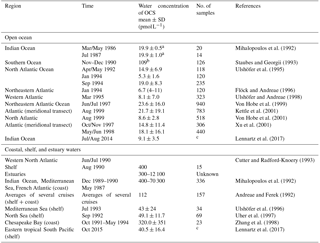
a Converted from ng L−1 with a molar mass of OCS of 60.07 g.
b Converted from ng S L−1 with a molar mass of S of 32.1 g.
c Continuous measurements.
2.4.1 Marine production and removal processes
The primary sources of OCS in the ocean are divided into photochemical and light-independent (dark) processes (Von Hobe et al., 2001; Uher and Andreae, 1997). The primary sink is uncatalyzed hydrolysis (Fig. 6; Elliott et al., 1989). Evidence indicates that these processes can regulate OCS concentrations in the ocean surface mixed layer, with diverging conclusions on the magnitude and global significance of marine OCS emissions (Launois et al., 2015a). We use the Lennartz et al. (2017) budget here because the emission estimate is based on a model consistent with the majority of sea surface concentration measurements.
Global estimates of photoproduction for the surface mixed layer can range by up to a factor of 40 depending on the methodology used (Fig. 9). The heart of the problem is a limited knowledge of the magnitude, spectral characteristics, and spatial and temporal variability of the apparent quantum yield (AQY).
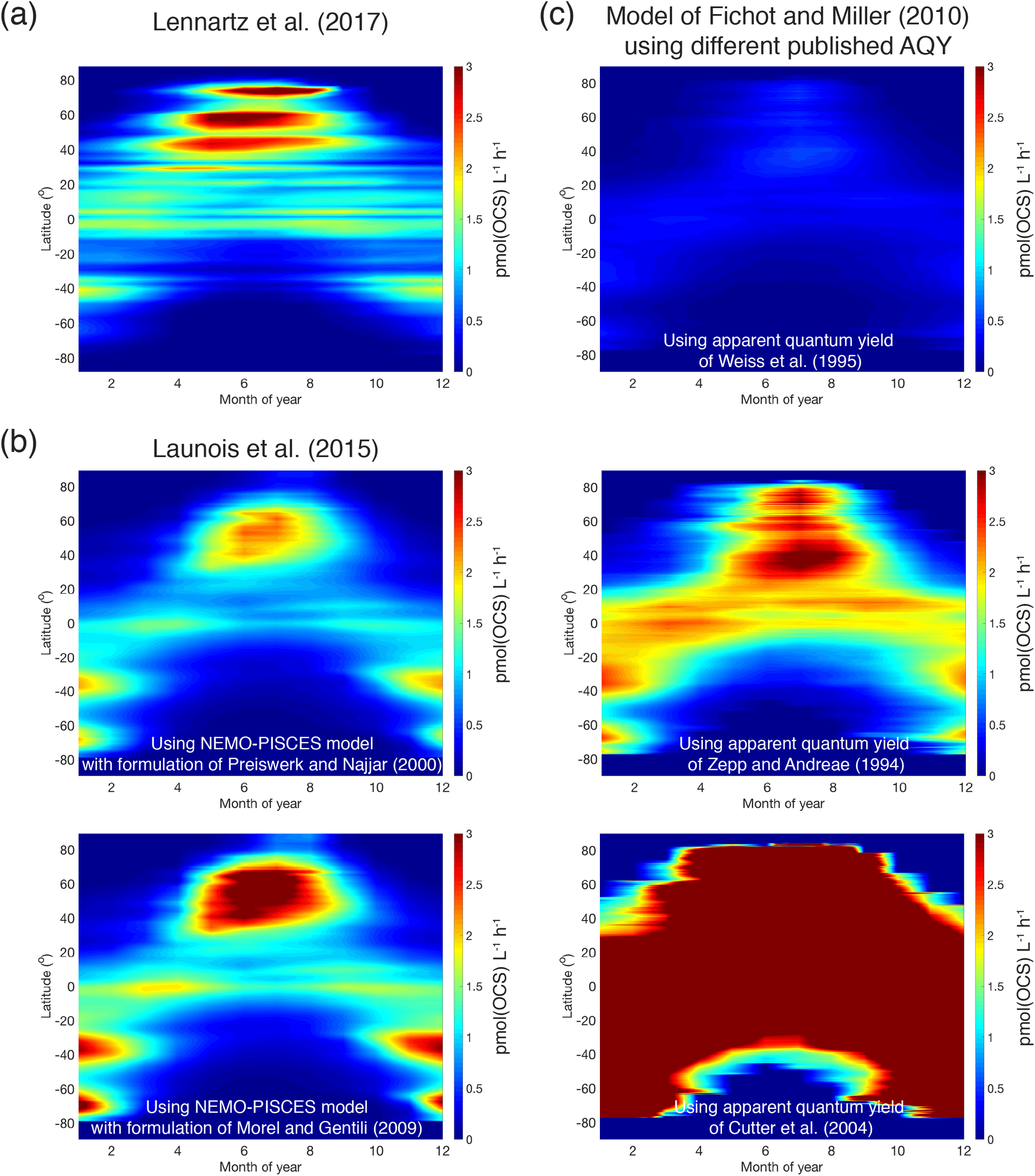
Figure 9Comparison of OCS photoproduction rates (averages for surface mixed layer, pmol(OCS) ) modeled using different approaches and demonstrating discrepancies between methods: (a) Hovmöller (latitude–time) plot of rates calculated using the approach described in Lennartz et al. (2017); (b) the same Hovmöller plot generated with the approach described in Launois et al. (2015a) and two different formulations for CDOM absorption coefficients from Preiswerk and Najjar (2000) and Morel and Gentili (2004); and (c) the same Hovmöller plots generated with the photochemical model of Fichot and Miller (2010) and the published spectral apparent quantum yields of Weiss et al. (1995), Zepp and Andreae (1994), and Cutter et al. (2004).
There is evidence for the role of biological processes (Flöck and Andreae, 1996) and for the involvement of radicals (Pos et al., 1998) in OCS production. Independent of a mechanism, only one parameterization for dark production is currently used in models (Von Hobe et al., 2001). Neither the direct precursor nor the global applicability of this parameterization is known. Despite these unknowns, the current gap in the top-down OCS budget (Sect. 3.1) is larger than the estimated ocean emissions, including uncertainties from process parameterization and in situ observations. This suggests that our estimates of OCS production in oceans will not close the gap in top-down OCS budgets.
Recommendations. Further studies should focus on generating a biochemical model for estimating oceanic OCS fluxes. Refining uncertainty bounds for OCS photoproduction could be facilitated by a comprehensive study of the variability of AQYs across contrasting marine environments, the use of a photochemical model that utilizes AQYs and facilitates calculations on a global scale, and the cross-validation of the depth-resolved modeled rates with direct in situ measurements. During nighttime, continuous concentration measurements from research vessels can be used to calculate dark production rates assuming an equilibrium between hydrolysis and dark production.
2.4.2 Indirect marine emissions
Indirect marine emissions from oxidation of the precursor gases CS2 and possibly dimethyl sulfide (DMS) were hypothesized to be on the same order of magnitude as or larger than direct ocean emissions of OCS (Chin and Davis, 1993; Watts, 2000; Kettle et al., 2002). Production and loss processes of CS2 in seawater are less well constrained than OCS production, and they include photoproduction, evidence for biological production (Xie et al., 1998, 1999), and a slow chemical sink (Elliott, 1990).
Measurements of CS2 in the surface ocean comprise several transects in the Atlantic and Pacific oceans with concentrations in the lower picomoles-per-liter range. Significantly larger concentrations have been found in coastal waters (Uher, 2006, and references therein). In laboratory experiments, Hynes et al. (1988) found that the OCS yield from CS2 increases with decreasing temperatures, suggesting larger OCS production from CS2 at high latitudes.
It is unclear if the ambient yield of OCS from DMS oxidation is globally important. The production of OCS from the oxidation of DMS by OH has been observed in several chamber experiments, all of which used the same technique and experimental chamber (Barnes et al., 1994, 1996; Patroescu et al., 1998; Arsene et al., 1999, 2001) with a molar yield of 0.7±0.2 %. These studies were carried out at precursor levels far exceeding those in the atmosphere (ppm), so the potential exists for radical–radical reactions that do not occur in nature. In addition, experiments took place in a quartz chamber on timescales that have potential for wall-mediated surface or heterogeneous reactions and using only a single total pressure and temperature (1000 mbar, 298 K). The mechanism and atmospheric relevance of OCS production from DMS remain highly uncertain.
Recommendations: To better constrain oceanic CS2 emissions, we suggest expanding surface concentration observations across various biogeochemical regimes and seasons. Using field observations, laboratory studies, and process models, we could characterize production processes and identify drivers and rates when calculating OCS emission estimates. Elucidating the production pathway and validating the atmospheric applicability of the reported OCS yields from DMS would require experiments at lower concentrations in a system that eliminates (or permits quantification of) wall-induced reactions.
2.5 Anthropogenic sources
Anthropogenic OCS sources include direct emissions of OCS and indirect sources from emissions of CS2. The dominant source is from rayon production (Campbell et al., 2015), while other large sources include coal combustion, aluminum smelting, pigment production, shipping, tire wear, vehicle emissions, and coke production (Blake et al., 2008; Chin and Davis, 1993; Du et al., 2016; Lee and Brimblecombe, 2016; Watts, 2000; Zumkehr et al., 2017).
All recent global atmospheric modeling studies have used the low estimate of 180 Gg S yr−1 from Kettle et al. (2002), which did not capture significant emissions from China. Updated globally gridded inventories are considerably higher: a bottom-up estimate of 223–586 Gg S yr−1 for 2012 (Zumkehr et al., 2018) and a top-down assessment of 230 to 350 Gg S yr−1 for 2011 to 2013 (Campbell et al., 2015). One reason for the gap between the two recent inventories is that the top-down study used an optimization approach in which the result was limited to the a priori range, 150 to 364 Gg S yr−1. Both datasets indicate that most anthropogenic sources are in Asia.
Biomass burning is generally accounted for as a category separate from anthropogenic emissions. Several airborne campaigns have observed increases in OCS concentrations in air masses from nearby burning events (Blake et al., 2008). The most recent estimate suggests that biofuels, open burning, and agriculture residue are 63, 26, and 11 % of the total OCS biomass burning emissions, respectively (Campbell et al., 2015).
Recommendations. Anthropogenic OCS emissions experience large year-to-year variation (Campbell et al., 2017a). Ambient OCS monitoring and on-site industry observations in Asia could observe the anthropogenic contribution over time. In particular, modern viscose-rayon factory emissions are necessary to capture the variability of emissions factors used to scale rayon production to OCS emissions using economic data.
2.6 Volcanic sources
OCS is emitted into the atmosphere by degassing magma, volcanic fumaroles, and geothermal fluids. OCS can be released at room temperature by volcanic ash (Rasmussen et al., 1982) and has been observed to be conservative in the atmospheric plume emitted by the Mount Erebus volcano up to tens of kilometers downwind of the volcanic source (Oppenheimer et al., 2010).
Using the linear relationship between the logarithm of the OCS / CO2 ratio in volcanic gases and temperature, the volcanic OCS contribution was determined from estimated CO2 emissions (Belviso et al., 1986). Here we calculate a revised temperature dependence of log[OCS / CO2] with additional data (Chiodini et al., 1991; Notsu and Toshiya, 2010; Sawyer et al., 2008; Symonds et al., 1992), as shown in Fig. 10. The compilation of measurements from 14 volcanoes shows that the former relationship from Belviso et al. (1986) overestimated the OCS / CO2 ratio of volcanic gases with emission temperatures from 110 to 400 ∘C, typical of extra-eruptive volcanoes. Even with this improved estimate, OCS emissions of extra-eruptive volcanoes are negligibly small and can definitely be discarded from the inventory of volcanic OCS emissions. Eruptive and post-eruptive volcanoes contribute almost all OCS emissions from volcanism.
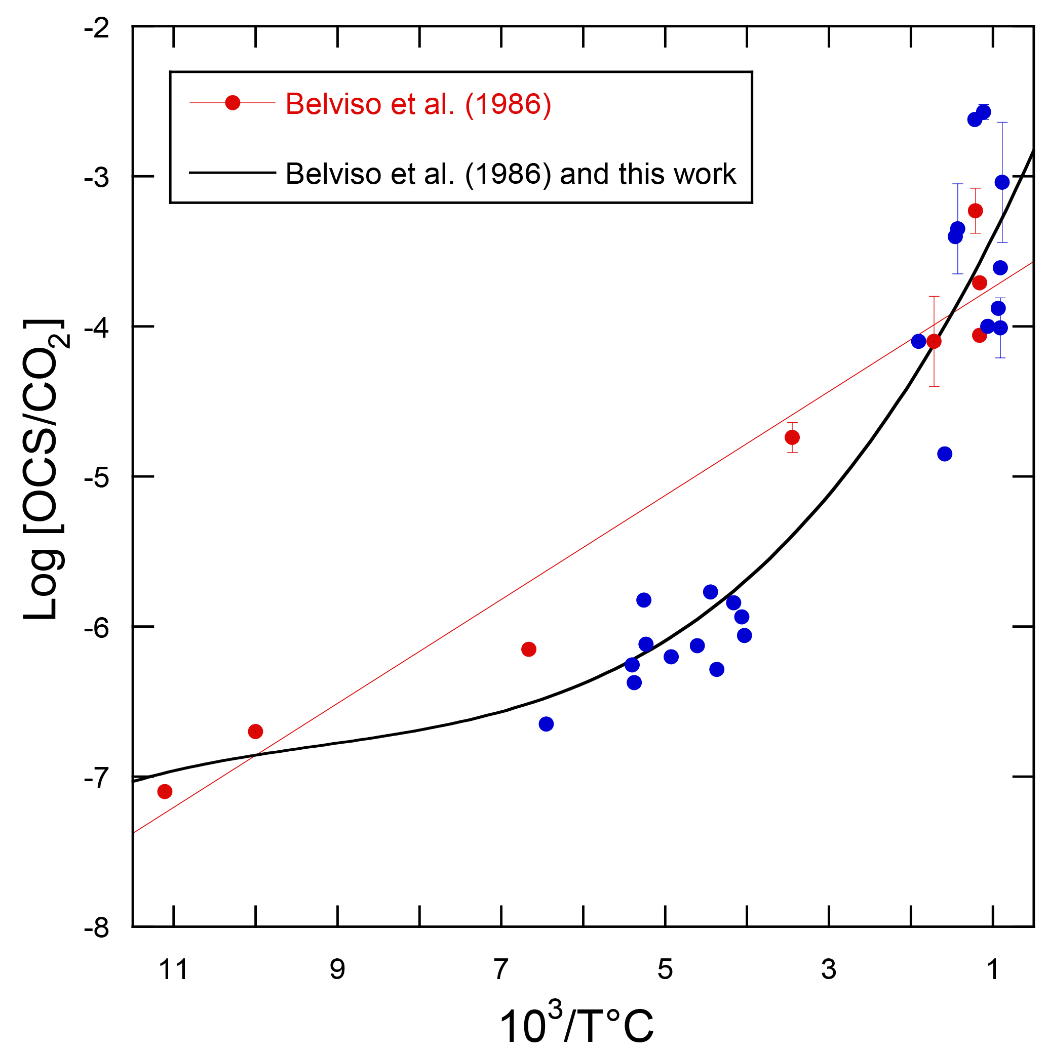
Figure 10Decimal logarithm of the OCS / CO2 ratios plotted against the reciprocal of the emission temperature of the gases for volcanoes. The red dots refer to the analytical data published by Belviso et al. (1986) and the red line corresponds to the linear model used in that study to evaluate the volcanic contribution to the atmospheric OCS budget. The blue dots refer to measurements published by others since 1986 (Chiodini et al., 1991; Notsu and Toshiya, 2010; Sawyer et al., 2008; Symonds et al., 1992). The better fit through all measurements is obtained using a polynomial of the third order (R2=0.89, n=31).
Recommendations. An updated inventory of eruptive volcanoes and a better assessment of their CO2 emissions will refine our understanding at a regional scale of the contribution of OCS from volcanoes. Special attention should be paid to the Ring of Fire off the Asian continent where satellites have observed significant atmospheric OCS enhancements.
2.7 Bottom-up OCS budget
We calculate a “bottom-up” global balance of OCS with several approaches, as presented in Table 4. Within the atmosphere, the tropospheric sink owing to oxidation by OH is estimated to be in the range 82–130 Gg S yr−1 (Berry et al., 2013; Kettle et al., 2002; Watts, 2000), and the stratospheric sink is in the range 30–80 Gg S yr−1, or 50±15 Gg S yr−1 (Barkley et al., 2008; Chin and Davis, 1995; Crutzen, 1976; Engel and Schmidt, 1994; Krysztofiak et al., 2015; Turco et al., 1980; Weisenstein et al., 1997). OCS concentrations are increasing roughly 0.5–1 ppt year−1 averaged over the last 10 years (Campbell et al., 2017a), suggesting approximately 2 to 5 Gg S yr−1 remains in the troposphere.
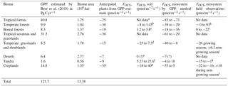
We build a budget for terrestrial biomes that relies on observations where available, and on estimates of carbon uptake where no data exists, as has been done previously (Campbell et al., 2008; Kettle et al., 2002; Suntharalingam et al., 2008). In Table 5, the estimated OCS uptake is first calculated from a GPP estimate and Eq. (1); then the net OCS flux is appraised by taking into account observed or estimated soil fluxes for each biome. The [CO2] and [OCS] are assumed to be 400 ppm and 500 ppt, respectively, and LRU is 1.16±0.2 for C4 plants (Stimler et al., 2010b) and 1.99±1.44 for C3 plants (Fig. 2). We further assume a 150-day growing season with 12 h of light per day for the purposes of converting between annual estimates of GPP and field measurements calculated in per-second units, though this obviously does not represent the diversity of biomes' carbon assimilation patterns. Additionally, we assume that plants in desert biomes photosynthesize using the C4 pathway. Converting annual estimated FCOS from an annual estimate to a per-second estimate is sensitive to our growing season assumption. The lack of soil OCS flux time series datasets makes a more sophisticated upscaling approach ineffective. Anticipated fluxes from soils and plants are therefore combined in this purposely simple method, scaled to the area of the biome extent, and presented in Table 4 as annual contributions to the atmospheric OCS budget.
Table 5GPP and OCS exchange estimates by biome.
a For the purpose of this estimate, we use the soil
fluxes from temperate forests.
b Range of values from Castro and Galloway (1991),
Steinbacher et al. (2004), White et al. (2010), and Yi et al. (2007).
c The average reported here is the average and 1 SD
from non-vegetated plots in a boreal forest, defined as plots having
less than 10 % vegetation cover (Simmons, 1999).
d Range from Whelan and Rhew (2016). The error estimate
here is different from the one reported because a different LRU was
used. Kitz et al. (2017) found soil-only OCS production of
+60 in an alpine grassland.
e In a laboratory incubation study, Whelan et al. (2016)
found that desert soils exhibit a very small uptake. No field
measurements have been published to our knowledge.
f The smaller production is from de Mello and Hines
(1994). The larger production is an average estimate from Fried et al. (1993).
g Post-harvest soil exchange estimate from the wheat
field (Billesbach et al., 2014) investigated further in Whelan and
Rhew (2015).
h See Table 1.
i From Simmons et al. (1999).
j Range from Whelan and Rhew (2016), encompassing observations of
a grass field by Yi and Wang (2011).
k Range reported in de Mello and Hines (1994), encompassing values
observed by a bog microcosm by Fried et al. (1993). No valid Arctic studies exist.
l High value for cotton, low value for wheat in Asaf
et al. (2013). Daily fluxes for a wheat field investigated by Billesbach
et al. (2014) were −21 during the growing season and +18 after harvest.
Agricultural soils have been shown to emit a large portion of OCS compared to
plant uptake under hot and dry conditions (Whelan et al., 2016; Whelan and
Rhew, 2015).
We use a range of OCS flux observations in picomoles of OCS per square meter per second for fresh and saline wetlands: −15 (de Mello and Hines, 1994) to +27 (Liu and Li, 2008) for freshwater wetlands and −9.5 (Li et al., 2016) to +60 (Whelan et al., 2013) for saltwater wetlands (Fig. 4). Marine and inland wetlands cover 660 and 9200×103 km2, respectively (Lehner and Döll, 2004). Performing a simple scaling exercise results in contributions of −140 to 250 and −6 to 40 Gg S yr−1 for fresh and saltwater wetlands, respectively, yielding a total range of −150 to 290 Gg S yr−1 (Table 4).
To determine the role of non-vascular plant communities to the atmospheric OCS loading, we leverage Eq. (1) and work that has already been done on their carbon balance. According to Elbert et al. (2012), the annual contribution is 3.9 Pg C yr−1. A [OCS] of 500 ppt, a [CO2] of 400 ppm, and a LRU of 1.1±0.5 (Gimeno et al., 2017) yield −8 to −21 Gg S yr−1.
To estimate the maximum possible source of lakes to the atmospheric OCS burden, we perform a simple estimation of the global OCS flux following the approach in MacIntyre et al. (1995) as
where gas transfer coefficient, k, is assumed to be constant at 0.54 m d−1 (Read et al., 2012); OCS concentration in the water, caq, is 90 pmol L−1 to 1.1 nmol L−1 (Richards et al., 1991); and OCS concentration in the surface water if it was in equilibrium with the above air, ceq, is calculated using Henry's law at global average temperature of 15 ∘C and global atmospheric OCS mixing ratio of 500 ppt. Accounting for the number of ice-free days in a year and total lake surface area per latitude (Downing et al., 2006), the range of possible COS burden from lakes to the atmosphere is reported here as 0.8 to 12 Gg S yr−1.
Lennartz et al. (2017) generated a direct estimate of direct OCS emissions from oceans as 130±80 Gg S yr−1. A molar yield of CS2 to OCS of 0.81–0.93 was established by Stickel et al. (1993) and Chin and Davis (1993), resulting in ocean OCS emissions from CS2 with an uncertainty of 20–80 Gg S yr−1. This uncertainty is from the emissions of CS2, not the molar yield, for which a globally constant factor is used. The global DMS oxidation source of OCS was estimated by Barnes et al. (1994) as 50.1–140.3 Gg S yr−1, and subsequent budgets contain only revisions according to updated DMS emissions (Kettle et al., 2002; Watts, 2000). We suggest that the uncertainty in the production of OCS from DMS is underestimated. Until these issues are resolved, we recommend that this term be removed as a source from future budgets, but retained as an uncertainty.
Bottom-up analysis of the global anthropogenic inventory indicates a source of 500±220 Gg S yr−1 for the year 2012 (Zumkehr et al., 2018). The large uncertainty is primarily due to limited observations of emission factors, particularly for the rayon, pulp, and paper industries. The most recent estimate of the biomass burning sources is 116±52 Gg S yr−1 (Campbell et al., 2015).
To calculate global volcanic OCS emissions, we first consider the range of global volcanic CO2 emission estimates of the five studies reviewed by Gerlach (2011) of 0.15–0.26 Pg yr−1, or 0.205±0.055 Pg yr−1. Assuming that the mean OCS / CO2 molar ratio of gases emitted by eruptive and post-eruptive volcanoes is (for emission temperatures in the range 525–1130 ∘C, see Fig. 10), the revised annual volcanic input of OCS into the troposphere is estimated to be in the range 25–43 Gg S yr−1.
Examining Table 4, we find large uncertainties in many global estimates, and some biome observations are completely absent. It has been suggested that ocean OCS production has been underestimated (Berry et al., 2013), and some research points to unaccounted-for anthropogenic sources (Zumkehr et al., 2018). The uncertainty in our ocean OCS production and/or the industry inventories does not necessarily capture the true range of OCS fluxes. Despite the large uncertainties of the global OCS budget, many applications of the OCS tracer have been attempted with success.
Recommendations. More observations in the ocean OCS source region and from industrial processes, particularly in Asia, are needed to further assess their actual magnitude and variation (Suntharalingam et al., 2008). Current leaf-based investigations need to be expanded to include water- or nutrient-stressed plants. Measurements from biomes with a complete lack of data, such as deserts and the entirety of the tropics, are desperately needed.
3.1 Top-down global OCS budgets
Top-down estimates use observed spatial and temporal gradients of OCS in the atmosphere to adjust independent surface fluxes, called the prior estimate. Constraints can be introduced to the results; e.g., Launois et al. (2015b) used flask measurement observations to optimize surface OCS flux components to obtain a closed global OCS budget. Other top-down estimates without this restriction found a missing source of about 600–800 Gg S yr−1 in the atmospheric budget of OCS (Berry et al., 2013; Glatthor et al., 2015; Kuai et al., 2015; Suntharalingam et al., 2008; Wang et al., 2016). This could be the result of missing oceanic sources, missing anthropogenic OCS sources from Asia, overestimated plant uptake, or a combination of factors.
Kuai et al. (2015) implied a large ocean OCS source over the Indo-Pacific region with the total ocean source budget consistent with the global budget proposed by Berry et al. (2013). The observations in Kuai et al. (2015) were estimated OCS surface fluxes from NASA's Tropospheric Emission Spectrometer (TES) ocean-only observations. A similar conclusion was obtained by Glatthor et al. (2015), who showed that the OCS global seasonal cycle observed by the Michelson Interferometer for Passive Atmospheric Sounding (MIPAS) was more consistent with the seasonal cycles modeled using the Berry et al. (2013) global budget than using the global budget proposed earlier by Kettle et al. (2002).
Most of the anthropogenic source is located in China, while most of the atmospheric OCS monitoring is located in North America (Campbell et al., 2015). The spatial separation allows regional applications of OCS to North America to control for most of the anthropogenic influence through observed boundary conditions (Campbell et al., 2008; Hilton et al., 2015, 2017). The anthropogenic source has large interannual variations (Campbell et al., 2015), which suggest that applications of the OCS tracer to inter-annual carbon cycle analysis will require careful consideration of anthropogenic variability.
Recommendations. The accuracy of OCS surface flux inversions can be improved by using simultaneous OCS observations from multiple satellites, e.g., TES and MIPAS, to provide more constraints on the OCS distribution in different parts of the atmosphere. Satellite products need to be compared to observations to determine how well the upper troposphere can reflect surface fluxes, e.g., long-term tower measurements, airborne eddy flux covariance, and atmospheric profiles. This effort is furthered by better estimates of surface fluxes, in particular observations of OCS emissions from the oceans where we assume a large source region might exist (Kuai et al., 2015) and where poorly described anthropogenic sources are located in Asia (Zumkehr et al., 2018).
3.2 Global and regional terrestrial GPP estimates
Here we describe work using OCS observations to assemble more information about ecosystem functioning on different scales. Estimates disagree in their diagnoses of global (Piao et al., 2013) and regional (Parazoo et al., 2015) GPP magnitude and spatial distribution in North America (Huntzinger et al., 2012), the Amazon (Restrepo-Coupe et al., 2017), and Southeast Asia (Ichii et al., 2013). Feeding observations of OCS uptake over land into transport models informs the spatial distribution and magnitude of GPP. With the suite of OCS flask and satellite data available, we describe studies that examine OCS fluxes with the top-down approach. Finally, we examine GPP estimates on very long temporal scales using the OCS ice core record.
3.2.1 Evaluating biosphere models
There are many uncertainties in evaluating biosphere models using OCS observations. Hilton et al. (2017) showed that the spatial placement of GPP dominates other uncertainty sources in the GPP tracer approach on a regional scale. Land surface models that placed the largest GPP in the Upper Midwest of the United States produced OCS plant fluxes that matched aircraft observations well for all estimates of OCS soil flux, OCS anthropogenic flux, and transport model boundary conditions. OCS plant fluxes derived from GPP models that place the largest GPP in the southeastern United States were not able to match aircraft-observed OCS for any combination of secondary OCS fluxes. Placement of the strongest North American GPP in the Upper Midwest is consistent with new ecosystem models from the Coupled Model Intercomparison Project Phase 6 (CMIP6) (Eyring et al., 2016) with space-based estimates from solar-induced fluorescence (SIF; Guanter et al., 2014; Parazoo et al., 2014). This result is encouraging for the potential of OCS to provide a directly observable tracer for GPP at regional scales.
Launois et al. (2015b) analyzed the potential of existing atmospheric OCS and CO2 mixing ratio measurements to evaluate model GPP biases. They used the simulated GPP from three global land surface model simulations from the TRENDY intercomparison (Sitch et al., 2015) and an atmospheric transport model. The amplitude and phase of the seasonal variations of atmospheric OCS appear mainly controlled by the vegetation OCS sink. This allows for bias recognition in the spatial and temporal patterns of the GPP. For instance, the ORCHIDEE GPP at high northern latitudes is overestimated, as revealed by a too-large OCS seasonal cycle at the Alert station (ALT, Canada) (Fig. 11). These results highlight the potential of current in situ OCS measurement to reveal model GPP and respiration biases.
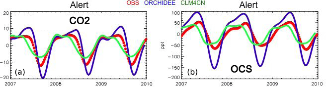
Figure 11Smoothed seasonal cycles of OCS (right) and CO2 (left) monthly mean mixing ratios, simulated at Alert station, Canada, obtained after removing the annual trends. Simulations are obtained with the LMDz transport model, using two flux scenarios for the vegetation uptake of OCS, calculated with the GPP of ORCHIDEE and CLM4CN models; the other OCS flux components are identical (see Launois et al. 2015). Observations (red) are from the NOAA/ESRL global monitoring network (Montzka et al., 2007) averaged from 2007 to 2010.
Recommendations. While current datasets can support or refute current land surface model GPP data products over North America, evaluating modeled surface GPP fluxes with OCS observations would benefit from a broader network of continuous OCS observations. Unfortunately, satellite data are not currently sensitive to concentrations at the surface. Maintaining a network of tall towers with continuous OCS measurements over more than one continent could, in conjunction with upper-troposphere measurements from satellites, provide the data needed to refine next-generation land surface models.
3.2.2 Long-term changes in carbon uptake
Ice core samples from the West Antarctic Ice Sheet Divide were used to produce a 54 300-year OCS record and an order-of-magnitude estimate of the change in GPP during the last glacial–interglacial transition (Aydin et al., 2016). Atmospheric OCS declined by 80 to 100 ppt during the last glacial–interglacial transition. Interpretation of these measurements with a simple box model suggests that GPP roughly doubled during the transition. This order-of-magnitude estimate is consistent with an ecosystem model that simulates 44 % growth in GPP over the same period (Prentice et al., 2011).
The ice core OCS record has also been used to explore variation in GPP over the past 2000 years. Observations show relative maxima at the peak of the Little Ice Age (Aydin et al., 2008). These data were used to estimate growth in GPP and were combined with other information to estimate the temperature sensitivity of pre-industrial CO2 fluxes for the terrestrial biosphere (Rubino et al., 2016).
Given that Earth system model projections have highly uncertain carbon–climate feedbacks (Friedlingstein et al., 2013), understanding of GPP in the current industrial era is needed to provide a benchmark for future model development. Firn air measurements and one-dimensional firn models have been used to show an increase in atmospheric OCS during most of the industrial era, with a decadal period of decline beginning in the 1990s (Montzka et al., 2004, 2007). The trend in the firn record has been interpreted to largely reflect the increase in industrial emissions, but it also suggests an increase in GPP during the 20th century of 31±5 %, which is consistent with some models (Campbell et al., 2017a).
Recommendations. Examining the polar differences in OCS over glacial–interglacial periods would provide additional evidence for interpreting changes in GPP. For such an analysis, ice core OCS observations from the Northern Hemisphere are needed.
3.3 OCS to probe variables other than GPP
OCS and CO2 uptake within plant leaves is partly regulated by the opening of stomata on leaf surfaces. Stomatal conductance is typically determined from combined estimates of transpiration, water vapor concentration, and leaf temperature. That approach can be particularly challenging at the canopy scale, where transpiration is difficult to distinguish from non-stomatal water fluxes (i.e., evaporation from soil and canopy surfaces) and to upscale from sap flux measurements (Wilson et al., 2001). Use of OCS uptake involves the similar but more tractable challenge of distinguishing the canopy OCS uptake from soil OCS uptake or emission, as in Wehr et al. (2017). OCS data can also look at changes in uptake activity when plants are grown in elevated CO2 environments (White et al., 2010; Sandoval-Soto et al., 2012). Use of OCS uptake may also be less sensitive to errors in leaf temperature, which is difficult to define and quantify at the canopy scale but may be improved by OCS measurements (Yang et al., 2018). However, leaf temperature may still enter the problem via estimation of mesophyll conductance and CA activity.
The use of OCS to study canopy and stomatal conductance is therefore promising, but it is so far represented mostly by very few studies (Wehr et al., 2017; Yang et al., 2018). Wehr et al. (2017) used OCS uptake to derive canopy stomatal conductance and hence transpiration in a temperate forest. Stomatal conductance was the rate-limiting diffusive step, and so its diel and seasonal patterns were retrievable from the canopy OCS uptake to within 6 % of independent estimates based on sensible and latent heat flux measurements (Fig. 12). OCS would be especially useful in humid environments or at night, when transpiration is too small to use other methods that rely on sap flow or heat flux (Campbell et al., 2017b). However, an independent estimate of CA activity and mesophyll conductance would be required.
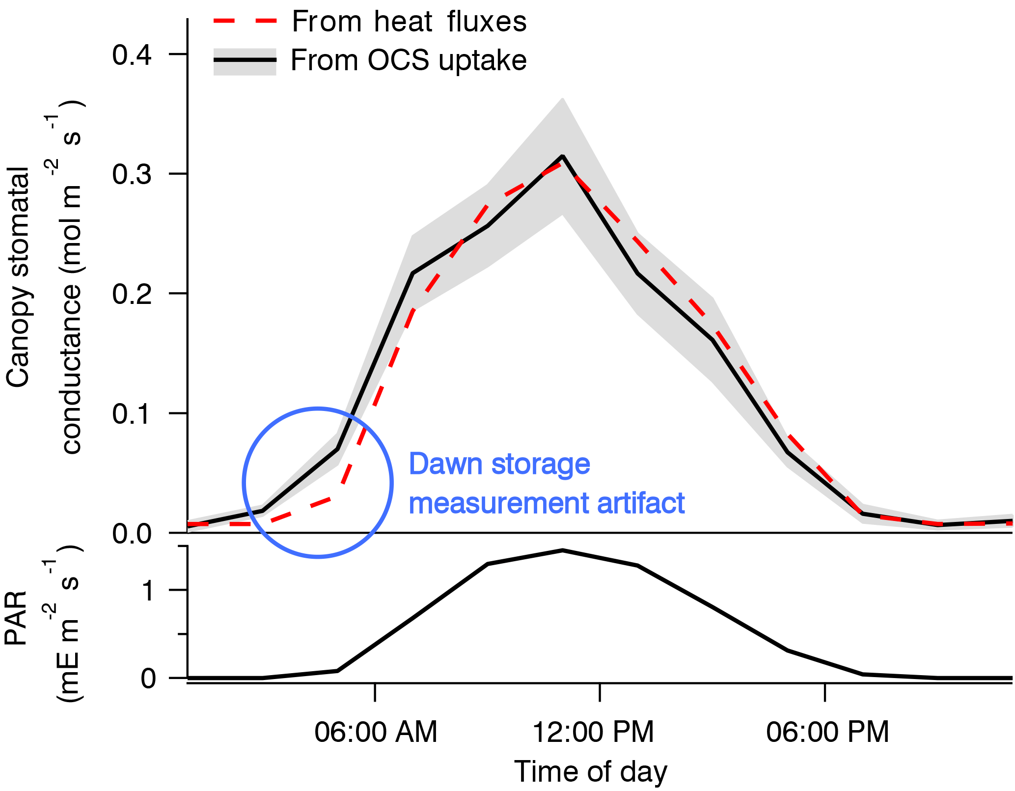
Figure 12Composite diel cycles of stomatal conductance derived from the OCS uptake (solid black line with gray bands) and from the sensible and latent heat fluxes (red dashed line), along with photosynthetically active radiation (PAR, bottom panel) for context, including May through October of 2012 and 2013. Lines connect the mean values of each 2 h bin. The gray bands depict standard errors in the means as estimated from the variability within each bin. Adapted from Wehr et al. (2017), which discusses the dawn storage measurement artifact indicated here by the blue circle.
Recommendations. OCS observations should be used to link plant physiological variables to one another. OCS fluxes are related to GPP via all three diffusive conductances, CA activity, transpiration, and the 18O isotope compositions of CO2 and H2O. The 18O connection results from the fact that CA promotes the exchange of oxygen isotopes between CO2 and liquid water in the leaves. Solar-induced fluorescence measurements could also be synergistic, as they relate to the photochemical aspect of photosynthesis, while OCS uptake relates to the gas transport aspect. So far, few research schemes have taken advantage of these relationships.
4.1 OCS satellite data products
Global OCS concentrations have been retrieved from several satellite instruments, including NASA's TES (Kuai et al., 2014), the Canadian Space Agency's Atmospheric Chemistry Experiment–Fourier Transform Spectrometer (ACE-FTS) (Boone et al., 2005), and the European Space Agency's MIPAS (von Clarmann et al., 2003; Glatthor et al., 2017) and Infrared Atmospheric Sounding Interferometer (IASI) (Camy-Peyret et al., 2017; Vincent and Dudhia, 2017). Among these instruments, TES and IASI are nadir-viewing instruments (i.e., looking downwards from space towards the surface), while ACE-FTS and MIPAS are limb scanners (i.e., looking through the atmosphere tangentially). Nadir measurements are less prone to cloud interference and provide good horizontal spatial resolution but coarse vertical resolution. Limb measurements provide better vertical resolution and higher sensitivity to tracer concentrations, but they are subject to a higher probability of cloud interference and poorer line-of-sight spatial resolution. Currently there are no satellite measurements that are strongly sensitive to OCS concentrations near the surface, where they are most needed to evaluate surface fluxes.
The standard TES OCS product is an average between 200 and 900 hPa, with maximum sensitivity to the mid-tropospheric value (Kuai et al., 2014; Fig. 13a). Currently, the TES OCS retrievals are available over ocean only for latitudes below 40∘, where the signal-to-noise ratio is higher (due to larger thermal contrasts) and the surface spectral emissivity can be easily specified. Comparisons with collocated airborne and ground measurements show that the current TES OCS data have an accuracy of 50–80 ppt, and the accuracy is improved to ∼7 ppt when averaged over 1 month (Kuai et al., 2014).

Figure 13Comparisons of the seasonal horizontal distribution of OCS retrievals. (a) TES averaged between 200 and 900 hPa, obtained using TES Level 2 swath OCS retrievals in 2006, averaged over four seasons (March to May, June to August, September to November, and December to February). (b) MIPAS (250 hPa), using MIPAS Level 2 swath retrievals from 2002 to 2011. The data in (a) and (b) have been averaged to the same 5∘ longitude × 4∘ latitude grid boxes and have been smoothed to a spatial resolution. (c) Two-month averages of IASI daytime OCS total column retrievals from 2014 with resolution , extracted from Vincent and Dudhia (2017). Missing data are represented by white areas in panels (a) and (b) and by gray areas in panel (c).
MIPAS retrievals from 7 to 25 km characterize the average OCS concentration in a thin layer (a few kilometers thick) around the corresponding tangent height. Currently, the MIPAS OCS product (Fig. 13b) provides pole-to-pole OCS concentrations at multiple levels in the upper troposphere and the stratosphere, which show an accuracy of ∼50 ppt against balloon-borne measurements. Figure 14 shows the summertime (June–August) latitudinal distribution of OCS observed by MIPAS (Glatthor et al., 2017).
IASI retrieves a single value for the total column OCS (Fig. 13c). Recently, Vincent and Dudhia (2017) reported the pole-to-pole global OCS retrieved from the IASI measurements. Their preliminary test showed that the seasonally averaged IASI OCS data vary consistently with ground measurements. The IASI OCS observations over land generally agree with the MIPAS observations, showing large sinks over South America and Africa. The high spatial resolution also reveals more clearly the land OCS sources over Asia, which are not seen in TES or MIPAS observations. Furthermore, the relatively low OCS abundance over the Intertropical Convergence Zone is only apparent in IASI data.
The ACE-FTS-reported OCS concentrations in the lower stratosphere are known to be 15 % lower than the balloon-borne measurements (Velazco et al., 2011) and ∼100 ppt lower than MIPAS OCS (Glatthor et al., 2017).

Figure 14Latitudinal distribution of OCS, observed by MIPAS. Extracted from Glatthor et al. (2017).
4.2 FTIR data
Ground-based FTIR retrievals of OCS are sensitive to the altitudes between the surface and 30 km, and can therefore more directly capture the variations near the surface compared to satellite data. There are two networks of FTIR spectrometers: the Network for the Detection of Atmospheric Composition Change (NDACC), recording the mid-infrared spectra including the OCS bands, and the Total Carbon Column Observing Network (TCCON), mainly focusing on the near infrared with only some sites including the OCS bands. The FTIR remote-sensing measurement is an indirect measurement and therefore needs to be calibrated to in situ observations to have the same scale when combining the datasets. For example, Wang et al. (2016) added an offset when comparing FTIR retrievals and HIAPER Pole-to-Pole Observations (HIPPO) to the same model. Published datasets exist for the periods 1993–1997 (Griffith et al., 1998), 1978–2002 (Rinsland et al., 2002), 2001–2014 (Kremser et al., 2015), 2005–2012 (Wang et al., 2016), and 1995–2015 (Lejeune et al., 2017) and by an airborne Fourier spectrometer for the period 1978–2005 (Coffey and Hannigan, 2010). Balloon-borne FTIR data are available starting in 1985 (Toon et al., 2018).
4.3 Tower and airborne data
Data are available from two kinds of airborne sampling: survey flights and atmospheric chemistry projects. OCS measurements from aircraft began in the late 1980s, using both in situ and flask collection with subsequent analysis by GC-MS (e.g., Bandy et al., 1992, 1993; Hoell et al., 1993; Thornton et al., 1996; Blake et al., 2008, etc). The airborne survey flight data are designed to sample background air at set locations on a regular basis over long time periods and are part of the NOAA/ESRL/GMD Global Greenhouse Gas Reference Network's aircraft program (http://www.esrl.noaa.gov/gmd/ccgg/aircraft/index.html, last access: 6 June 2018; an update of results published in Montzka et al., 2007). This data collection started in 1999 at a range of locations and has been used extensively in analysis of the continental US carbon budget (e.g., Campbell et al., 2008; Hilton et al., 2017). OCS has been measured at 10 globally distributed sites in the AGAGE network using the MEDUSA GC-MS. The data for the Jungfraujoch site are presented in Lejeune et al. (2017). Larger-spatial-scale, shorter-time-interval survey flights include the HIPPO (2009–2011) and ATom (2016–2018) airborne programs, which predominantly sample OCS over remote marine locations. Atmospheric chemistry flights are designed to understand chemical processing and pollution transport and include sampling as part of pollution transport across the Pacific (e.g., Pacific Exploratory Mission–West A (PEM-A); Thornton et al., 1996) or Transport and Chemical Evolution over the Pacific experiment (TRACE-P), which sampled Asian outflow dominated by anthropogenic OCS emissions in 2001 (Blake et al., 2004). Other projects included sampling of OCS over continents (e.g., over the US in 2004; Blake et al., 2008).
OCS measurements have been made from tall towers using flasks and subsequent analysis by GC-MS. Most long-term tall-tower observations have been conducted as part of the NOAA/ESRL/GMD tower network (Montzka et al., 2007). These data from 11–12 sites include continuous sampling from 2000 onward at a daily or twice-daily time basis for most of the record.
4.4 Ecosystem-level data
Three approaches have been used to quantify ecosystem fluxes of OCS: chamber measurements, gradient measurements, and eddy flux covariance measurements. While researchers have been quantifying OCS measurements with chambers for decades, most field outings prior to 1990 used dynamic chambers with sulfur-free sweep air, artificially inducing high emissions (Castro and Galloway, 1991).
Measurements from towers have been made in a variety of ecosystems. An OCS analyzer capable of determining ambient OCS and CO2 concentrations at 10 Hz is commercially available (Kooijmans et al., 2016; Commane et al., 2013; Stimler et al., 2010a), allowing for eddy flux covariance measurements (Asaf et al., 2013; Billesbach et al., 2014; Commane et al., 2015; Wehr et al., 2017). With this powerful new tool, traditional methods of partitioning carbon fluxes over ecosystems can be directly compared to using OCS data as a proxy for GPP in situ. A few studies have made use of the gradient method (Berresheim and Vulcan, 1992; Blonquist et al., 2011; Rastogi et al., 2018).
4.5 Oceanic measurements
OCS measurements in the surface ocean comprise about 6000 ship-based measurements. These samples are usually taken at a depth of 0–5 m below the ocean surface and analyzed by gas chromatography with various detectors or off-axis integrated cavity output spectrometry. Table 3 gives an overview on available measurements. A central database for ship-based OCS measurements is desired to derive global patterns and facilitate model comparison. Measurements of the precursor gas CS2 are scarcer than OCS measurements. Samples for CS2 are taken usually in a similar way to OCS samples from the same depth range and analyzed using gas chromatography and mass spectrometry detection.
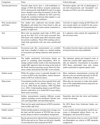
4.6 Firn and ice core records
Different hydrolysis rates apply for OCS trapped in bubbly ice vs. clathrate (bubble-free) ice. Some ice core material is not suitable for OCS analysis because the environment was too warm for long periods and OCS was hydrolyzed at high rates for thousands of years. Aydin et al. (2014, 2016) developed the necessary corrections to take into account OCS hydrolysis within the ice core bubbles. Corrected data are published for Taylor Dome, the West Antarctic Ice Sheet Divide, and Siple Dome (Aydin et al., 2016). Firn data are available for more recent time periods (Montzka et al., 2004; Sturges et al., 2001).
On the global scale, top-down estimates suggest a large missing source or overestimated sink of OCS. The available ocean water OCS measurements have not revealed a large enough OCS source to close the budget gap. This review concludes that the DMS source contribution for ocean OCS estimations should be considered only as a source of uncertainty until further experiments can be performed under conditions more similar to ambient air. Anthropogenic OCS estimates would benefit greatly from CS2 and OCS observations from rayon factories, particularly in Asia. Unaccounted-for domestic coal combustion in Asia may also play a significant role. To improve the robustness of the large-plant-sink estimate, observing OCS uptake in plants that are water or nutrient stressed may effect OCS exchange closer to the natural environment.
For regional-scale studies, aircraft profiles or flux measurements could help substantially with the OCS budget. We will need to quantify soil OCS fluxes in periodically hot and dry regions. Boreal and Arctic regions must take into account OCS fluxes from freshwater as well as bryophytes. Studies in tall forests require a more in-depth treatment of canopy-dwelling organisms, such as mosses and lichen.
Our overall understanding of the elements of the budget are summarized in Table 6. Several types of observations are needed to link the observed ground fluxes and the atmospheric satellite data, for example, FTIR measurements and AirCore campaigns. Ground OCS observations can also be applied in regions where current satellite coverage is poor, such as the tropics. Creating a global OCS data product and a coordinated tall-tower network generating continuous, calibrated concentration data will provide the information we need to close the global OCS budget and create an OCS-based estimate of global GPP.
All underlying data sets can be found in Sect. 4.
The authors declare that they have no conflict of interest.
This review was initiated at a workshop, “The biosphere–atmosphere
exchange and global budget of carbonyl sulfide”, held in
Hyytiälä, Finland, on 5–9 September 2016. The authors would
like to thank Colm Sweeney, Joost de Gouw, Mark Zahniser, Grayson Badgley, Leander Anderegg, Ian Baker, Ben Miller, Murat Aydin, and James Chalfant for helpful
discussion and data sharing. We acknowledge the integrative
activities through an OCS/CO2/SIF workshop funded by the
Keck Institute of Space Studies. Funding to support this work
included the following: Mary E. Whelan was supported by a National
Science Foundation (NSF) postdoctoral fellowship #1433257;
Mary E. Whelan and J. Elliott Campbell were supported by NSF grant
#1600109; Eric S. Saltzman was supported by NSF OPP-1142517;
Georg Wohlfahrt, Felix M. Spielmann, and Florian Kitz acknowledge
support by the Austrian Science Fund, FWF project
#P27176-B16, and the Tyrolean Science fund project
#UNI-0404/1801; Huilin Chen was supported by NOAA contract
NA13OAR4310082; Timo Vesala, Ivan Mammarella, and Kukka-Maaria Erkkilä were supported by the Academy of Finland Centre of
Excellence grant #307331, Academy Professor projects #284701
and #282842, ICOS-Finland #281255, and CARB-ARC #286190;
Ulli Seibt and Wu Sun were supported by NSF grant #1455381; Julia
Marshall was supported by the DFG, Project MA 6668/1-1.;
Teresa E. Gimeno and Lisa Wingate received funding from the
IdEx postdoctoral program of the Université de Bordeaux and
by a Marie Skłodowska-Curie Intra-European Fellowship, grant
agreement #653223; Lisa Wingate and Thomas Launois received
funding from the European Research Council under the European
Union's Seventh Framework Programme, FP7/2007-2013, grant agreement
#338264; Jérôme Ogée received funding from the
Agence National de la Recherche, ANR award #ANR-13-BS06- 0005-01;
Yoko Katayama received a Grant-in Aid for Scientific Research
(#18310020, #23310051, #16H05884, #17H06105,
#17J08979) from the Ministry of Education, Culture, Sport,
Science and Technology, Japan; Dan Yakir was supported by the
MINERVA foundation and the Israel Science Foundation (ISF); and the
European Geosciences Union and Aerodyne Research, Inc., provided
financial support to enable young researchers to attend the workshop
from which this article emerged.
Edited by: Sönke Zaehle
Reviewed by: Maarten Krol and Dennis Baldocchi
Andreae, M. O. and Ferek, R. J.: Photochemical production of carbonyl sulfide in seawater and its emission to the atmosphere, Global Biogeochem. Cy., 6, 175–183, 1992.
Aneja, V. P., Overton, J. H., and Aneja, A. P.: Emission Survey of Biogenic Sulfur Flux from Terrestrial Surfaces, JAPCA J. Air Waste Ma., 31, 256–258, 1981.
Arsene, C., Barnes, I., and Becker, K. H.: FT-IR product study of the photo-oxidation of dimethyl sulfide: Temperature and O2 partial pressure dependence, Phys. Chem. Chem. Phys., 1, 5463–5470, 1999.
Arsene, C., Barnes, I., Becker, K. H., and Mocanu, R.: FT-IR product study on the photo-oxidation of dimethyl sulphide in the presence of NOx – temperature dependence, Atmos. Environ., 35, 3769–3780, 2001.
Asaf, D., Rotenberg, E., Tatarinov, F., Dicken, U., Montzka, S. A., and Yakir, D.: Ecosystem photosynthesis inferred from measurements of carbonyl sulphide flux, Nat. Geosci., 6, 186–190, 2013.
Aydin, M., Williams, M. B., Tatum, C., and Saltzman, E. S.: Carbonyl sulfide in air extracted from a South Pole ice core: a 2000 year record, Atmos. Chem. Phys., 8, 7533–7542, https://doi.org/10.5194/acp-8-7533-2008, 2008.
Aydin, M., Fudge, T. J., Verhulst, K. R., Nicewonger, M. R., Waddington, E. D., and Saltzman, E. S.: Carbonyl sulfide hydrolysis in Antarctic ice cores and an atmospheric history for the last 8000 years, J. Geophys. Res.-Atmos., 119, 8500–8514, https://doi.org/10.1002/2014JD021618, 2014.
Aydin, M., Campbell, J. E., Fudge, T. J., Cuffey, K. M., Nicewonger, M. R., Verhulst, K. R., and Saltzman, E. S.: Changes in atmospheric carbonyl sulfide over the last 54 000 years inferred from measurements in Antarctic ice cores, J. Geophys. Res.-Atmos., 121, 1943–1954, https://doi.org/10.1002/2015JD024235, 2016.
Bandy, A. R., Thornton, D. C., Scott, D. L., Lalevic, M., Lewin, E. E., and Driedger, A. R.: A time series for carbonyl sulfide in the Northern Hemisphere, J. Atmos. Chem., 14, 527–534, 1992.
Bandy, A. R., Thornton, D. C., and Driedger, A. R.: Airborne measurements of sulfur dioxide, dimethyl sulfide, carbon disulfide, and carbonyl sulfide by isotope dilution gas chromatography/mass spectrometry, J. Geophys. Res., 98, 23423–23433, 1993.
Barkley, M. P., Palmer, P. I., Boone, C. D., Bernath, P. F., and Suntharalingam, P.: Global distributions of carbonyl sulfide in the upper troposphere and stratosphere, Geophys. Res. Lett., 35, L14810, https://doi.org/10.1029/2008GL034270, 2008.
Barnes, I., Becker, K. H., and Patroescu, I.: The tropospheric oxidation of dimethyl sulfide: A new source of carbonyl sulfide, Geophys. Res. Lett., 21, 2389–2392, 1994.
Barnes, I., Becker, K. H., and Patroescu, I.: FTIR product study of the OH initiated oxidation of dimethyl sulphide: Observation of carbonyl sulphide and dimethyl sulphoxide, Atmos. Environ., 30, 1805–1814, 1996.
Beer, C., Reichstein, M., Tomelleri, E., Ciais, P., Jung, M., Carvalhais, N., Rödenbeck, C., Arain, M. A., Baldocchi, D., and Bonan, G. B.: Terrestrial gross carbon dioxide uptake: global distribution and covariation with climate, Science, 329, 834–838, 2010.
Belviso, S., Nguyen, B. C., and Allard, P.: Estimate of carbonyl sulfide (OCS) volcanic source strength deduced from OCS/CO2 ratios in volcanic gases, Geophys. Res. Lett., 13, 133–136, 1986.
Belviso, S., Mihalopoulos, N., and Nguyen, B. C.: The supersaturation of carbonyl sulfide (OCS) in rain waters, Atmos. Environ., 21, 1363–1367, 1989.
Belviso, S., Schmidt, M., Yver, C., Ramonet, M., Gros, V., and Launois, T.: Strong similarities between night-time deposition velocities of carbonyl sulphide and molecular hydrogen inferred from semi-continuous atmospheric observations in Gif-sur-Yvette, Paris region, Tellus B, 65, 20719, https://doi.org/10.3402/tellusb.v65i0.20719, 2013.
Belviso, S., Reiter, I. M., Loubet, B., Gros, V., Lathière, J., Montagne, D., Delmotte, M., Ramonet, M., Kalogridis, C., Lebegue, B., Bonnaire, N., Kazan, V., Gauquelin, T., Fernandez, C., and Genty, B.: A top-down approach of surface carbonyl sulfide exchange by a Mediterranean oak forest ecosystem in southern France, Atmos. Chem. Phys., 16, 14909–14923, https://doi.org/10.5194/acp-16-14909-2016, 2016.
Berkelhammer, M., Asaf, D., Still, C., Montzka, S., Noone, D., Gupta, M., Provencal, R., Chen, H., and Yakir, D.: Constraining surface carbon fluxes using in situ measurements of carbonyl sulfide and carbon dioxide, Global Biogeochem. Cy., 28, 161–179, 2014.
Berresheim, H. and Vulcan, V. D.: Vertical distributions of COS, CS2, DMS and other sulfur compounds in a loblolly pine forest, Atmos. Environ. A-Gen., 26, 2031–2036, 1992.
Berry, J., Wolf, A., Campbell, J. E., Baker, I., Blake, N., Blake, D., Denning, A. S., Kawa, S. R., Montzka, S. A., Seibt, U., Stimler, K., Yakir, D., and Zhu, Z.: A coupled model of the global cycles of carbonyl sulfide and CO2: A possible new window on the carbon cycle, J. Geophys. Res.-Biogeo., 118, 842–852, 2013.
Bezsudnova, E. Y., Sorokin, D. Y., Tikhonova, T. V., and Popov, V. O.: Thiocyanate hydrolase, the primary enzyme initiating thiocyanate degradation in the novel obligately chemolithoautotrophic halophilic sulfur-oxidizing bacterium Thiohalophilus thiocyanoxidans, BBA-Proteins Proteom., 1774, 1563–1570, 2007.
Billesbach, D. P., Berry, J. A., Seibt, U., Maseyk, K., Torn, M. S., Fischer, M. L., Abu-Naser, M., and Campbell, J. E.: Growing season eddy covariance measurements of carbonyl sulfide and CO2 fluxes: COS and CO2 relationships in Southern Great Plains winter wheat, Agr. Forest Meteorol., 184, 48–55, 2014.
Blake, N. J., Streets, D. G., Woo, J.-H., Simpson, I. J., Green, J., Meinardi, S., Kita, K., Atlas, E., Fuelberg, H. E., Sachse, G., Avery, M. A., Vay, S. A., Talbot, R. W., Dibb, J. E., Bandy, A. R., Thornton, D. C., Rowland, F. S., and Blake, D. R.: Carbonyl sulfide and carbon disulfide: Large-scale distributions over the western Pacific and emissions from Asia during TRACE-P, J. Geophys. Res., 109, D15S05, https://doi.org/10.1029/2003JD004259, 2004.
Blake, N. J., Campbell, J. E., Vay, S. A., Fuelberg, H. E., Huey, L. G., Sachse, G., Meinardi, S., Beyersdorf, A., Baker, A., Barletta, B., Midyett, J., Doezema, L., Kamboures, M., McAdams, J., Novak, B., Rowland, F. S., and Blake, D. R.: Carbonyl sulfide (OCS): Large-scale distributions over North America during INTEX-NA and relationship to CO2, J. Geophys. Res.-Atmos., 113, D15S05, https://doi.org/10.1029/2007JD009163, 2008.
Blezinger, S., Wilhelm, C., and Kesselmeier, J.: Enzymatic consumption of carbonyl sulfide (COS) by marine algae, Biogeochemistry, 48, 185–197, 2000.
Bloem, E., Haneklaus, S., Kesselmeier, J., and Schnug, E.: Sulfur fertilization and fungal infections affect the exchange of H2S and COS from agricultural crops, J. Agr. Food Chem., 60, 7588–7596, 2012.
Blonquist, J. M., Montzka, S. A., Munger, J. W., Yakir, D., Desai, A. R., Dragoni, D., Griffis, T. J., Monson, R. K., Scott, R. L., and Bowling, D. R.: The potential of carbonyl sulfide as a proxy for gross primary production at flux tower sites, J. Geophys. Res.-Biogeo., 116, 1–18, 2011.
Boone, C. D., Nassar, R., Walker, K. A., Rochon, Y., McLeod, S. D., Rinsland, C. P., and Bernath, P. F.: Retrievals for the atmospheric chemistry experiment Fourier-transform spectrometer, Appl. Optics, 44, 7218–7231, 2005.
Brühl, C., Lelieveld, J., Crutzen, P. J., and Tost, H.: The role of carbonyl sulphide as a source of stratospheric sulphate aerosol and its impact on climate, Atmos. Chem. Phys., 12, 1239–1253, https://doi.org/10.5194/acp-12-1239-2012, 2012.
Bunk, R., Behrendt, T., Yi, Z., Andreae, M. O., and Kesselmeier, J.: Exchange of carbonyl sulfide (OCS) between soils and atmosphere under various CO2 concentrations, J. Geophys. Res.-Biogeo., 109, D15S05, https://doi.org/10.1002/2016JG003678, 2017.
Campbell, J. E., Carmichael, G. R., Chai, T., Mena-Carrasco, M., Tang, Y., Blake, D. R., Blake, N. J., Vay, S. A., Collatz, G. J., Baker, I., Berry, J. A., Montzka, S. A., Sweeney, C., Schnoor, J. L., and Stanier, C. O.: Photosynthetic control of atmospheric carbonyl sulfide during the growing season, Science, 322, 1085–1088, 2008.
Campbell, J. E., Whelan, M. E., Seibt, U., Smith, S. J., Berry, J. A., and Hilton, T. W.: Atmospheric carbonyl sulfide sources from anthropogenic activity: Implications for carbon cycle constraints, Geophys. Res. Lett., https://doi.org/10.1002/2015GL063445, 2015.
Campbell, J. E., Berry, J. A., Seibt, U., Smith, S. J., Montzka, S. A., Launois, T., Belviso, S., Bopp, L., and Laine, M.: Large historical growth in global terrestrial gross primary production, Nature, 544, 84–87, 2017a.
Campbell, J. E., Whelan, M. E., Berry, J. A., Hilton, T. W., Zumkehr, A., Stinecipher, J., Lu, Y., Kornfeld, A., Seibt, U., Dawson, T. E., Montzka, S. A., Baker, I. T., Kulkarni, S., Wang, Y., Herndon, S. C., Zahniser, M. S., Commane, R., and Loik, M. E.: Plant Uptake of Atmospheric Carbonyl Sulfide in Coast Redwood Forests, J. Geophys. Res.-Biogeo., 122, 3391–3404, https://doi.org/10.1002/2016JG003703, 2017b.
Camy-Peyret, C., Liuzzi, G., Masiello, G., Serio, C., Venafra, S., and Montzka, S. A.: Assessment of IASI capability for retrieving carbonyl sulphide (OCS), J. Quant. Spectrosc. Ra., 201, 197–208, 2017.
Castro, M. S. and Galloway, J. N.: A comparison of sulfur-free and ambient air enclosure techniques for measuring the exchange of reduced sulfur gases between soils and the atmosphere, J. Geophys. Res., 96, 15427–15437, 1991.
Chin, M. and Davis, D. D.: Global sources and sinks of OCS and CS2 and their distributions, Global Biogeochem. Cy., 7, 321–337, 1993.
Chin, M. and Davis, D. D.: A reanalysis of carbonyl sulfide as a source of stratospheric background sulfur aerosol, J. Geophys. Res., 100, 8993–9005, 1995.
Chiodini, G., Cioni, R., Raco, B., and Scandiffio, G.: Carbonyl sulphide (OCS) in geothermal fluids: An example from the Larderello field (Italy), Geothermics, 20, 319–327, 1991.
Coffey, M. T. and Hannigan, J. W.: The temporal trend of stratospheric carbonyl sulfide, J. Atmos. Chem., 67, 61–70, https://doi.org/10.1007/s10874-011-9203-4, 2010.
Commane, R., Herndon, S. C., Zahniser, M. S., Lerner, B. M., McManus, J. B., Munger, J. W., Nelson, D. D., and Wofsy, S. C.: Carbonyl sulfide in the planetary boundary layer: Coastal and continental influences, J. Geophys. Res.-Atmos., 118, 8001–8009, 2013.
Commane, R., Meredith, L. K., Baker, I. T., Berry, J. A., Munger, J. W., Montzka, S. A., Templer, P. H., Juice, S. M., Zahniser, M. S., and Wofsy, S. C.: Seasonal fluxes of carbonyl sulfide in a midlatitude forest, P. Natl. Acad. Sci. USA, 112, 14162–14167, 2015.
Crutzen, P. J.: The possible importance of CSO for the sulfate layer of the stratosphere, Geophys. Res. Lett., 3, 73–76, 1976.
Crutzen, P. J.: Albedo Enhancement by Stratospheric Sulfur Injections: A Contribution to Resolve a Policy Dilemma?, Climatic Change, 77, 211–219, 2006.
Cutter, G. A. and Radford-Knoery, J.: Carbonyl sulfide in two estuaries and shelf waters of the western North Atlantic Ocean, Mar. Chem., 43, 225–233, 1993.
Cutter, G. A., Cutter, L. S., and Filippino, K. C.: Sources and cycling of carbonyl sulfide in the Sargasso Sea, Limnol. Oceanogr., 49, 555–565, 2004.
DeLaune, R. D., Devai, I., and Lindau, C. W.: Flux of reduced sulfur gases along a salinity gradient in Louisiana coastal marshes, Estuar. Coast. Shelf S., 54, 1003–1011, 2002.
de Mello, W. Z. and Hines, M. E.: Application of static and dynamic enclosures for determining dimethyl sulfide and carbonyl sulfide exchange in Sphagnum peatlands: Implications for the magnitude and direction of flux, J. Geophys. Res., 99, 14601–14607, 1994.
Deprez, P. P., Franzmann, P. D., and Burton, H. R.: Determination of reduced sulfur gases in antarctic lakes and seawater by gas chromatography after solid adsorbent preconcentration, J. Chromatogr. A, 362, 9–21, 1986.
Devai, I. and DeLaune, R. D.: Trapping Efficiency of Various Solid Adsorbents for Sampling and Quantitative Gas Chromatographic Analysis of Carbonyl Sulfide, Anal. Lett., 30, 187–198, 1997.
Downing, J. A., Prairie, Y. T., Cole, J. J., Duarte, C. M., Tranvik, L. J., Striegl, R. G., McDowell, W. H., Kortelainen, P., Caraco, N. F., Melack, J. M., and Middleburg, J. J.: The global abundance and size distribution of lakes, ponds, and impoundments, Limnol. Oceanogr., 51, 2388–2397, 2006.
Du, Q., Zhang, C., Mu, Y., Cheng, Y., Zhang, Y., Liu, C., Song, M., Tian, D., Liu, P., Liu, J., Xue, C., and Ye, C.: An important missing source of atmospheric carbonyl sulfide: Domestic coal combustion, Geophys. Res. Lett., 43, 8720–8727, 2016.
Du, Q., Mu, Y., Zhang, C., Liu, J., Zhang, Y., and Liu, C.: Photochemical production of carbonyl sulfide, carbon disulfide and dimethyl sulfide in a lake water, J. Environ. Sci., 51, 146–156, 2017.
Elbert, W., Weber, B., Burrows, S., Steinkamp, J., Büdel, B., Andreae, M. O., and Pöschl, U.: Contribution of cryptogamic covers to the global cycles of carbon and nitrogen, Nat. Geosci., 5, 459–462, 2012.
Elliott, S.: Effect of hydrogen peroxide on the alkaline hydrolysis of carbon disulfide, Environ. Sci. Technol., 24, 264–267, 1990.
Elliott, S., Lu, E., and Rowland, F. S.: Rates and mechanisms for the hydrolysis of carbonyl sulfide in natural waters, Environ. Sci. Technol., 23, 458–461, 1989.
Engel, A. and Schmidt, U.: Vertical profile measurements of carbonylsulfide in the stratosphere, Geophys. Res. Lett., 21, 2219–2222, 1994.
Eyring, V., Bony, S., Meehl, G. A., Senior, C. A., Stevens, B., Stouffer, R. J., and Taylor, K. E.: Overview of the Coupled Model Intercomparison Project Phase 6 (CMIP6) experimental design and organization, Geosci. Model Dev., 9, 1937–1958, https://doi.org/10.5194/gmd-9-1937-2016, 2016.
Ferek, R. J. and Andreae, M. O.: Photochemical production of carbonyl sulphide in marine surface waters, Nature, 307, 148–150, 1984.
Fichot, C. G. and Miller, W. L.: An approach to quantify depth-resolved marine photochemical fluxes using remote sensing: Application to carbon monoxide (CO) photoproduction, Remote Sens. Environ., 114, 1363–1377, 2010.
Flöck, O. R. and Andreae, M. O.: Photochemical and non-photochemical formation and destruction of carbonyl sulfide and methyl mercaptan in ocean waters, Mar. Chem., 54, 11–26, 1996.
Flöck, O. R., Andreae, M. O., and Dräger, M.: Environmentally relevant precursors of carbonyl sulfide in aquatic systems, Mar. Chem., 59, 71–85, 1997.
Fried, A., Klinger, L. F., and Iii, D. J. E.: Atmospheric carbonyl sulfide exchange in bog microcosms, Geophys. Res. Lett., 20, 129–132, 1993.
Friedlingstein, P., Meinshausen, M., Arora, V. K., Jones, C. D., Anav, A., Liddicoat, S. K., and Knutti, R.: Uncertainties in CMIP5 climate projections due to carbon cycle feedbacks, J. Climate, 27, 511–526, 2013.
Fritz, M. and Bachofen, R.: Volatile organic sulfur compounds in a meromictic alpine lake, Acta Hydroch. Hydrob., 28, 185–192, 2000.
Geng, C. and Mu, Y.: Carbonyl sulfide and dimethyl sulfide exchange between lawn and the atmosphere, J. Geophys. Res.-Atmos., 109, D12302, https://doi.org/10.1029/2003JD004492, 2004.
Gerdel, K., Spielmann, F. M., Hammerle, A., and Wohlfahrt, G.: Eddy covariance carbonyl sulfide flux measurements with a quantum cascade laser absorption spectrometer, Atmos. Meas. Tech., 10, 3525–3537, https://doi.org/10.5194/amt-10-3525-2017, 2017.
Gerlach, T.: Volcanic vs. anthropogenic carbon dioxide, Eos T. Am. Geophys. Un., 92, 201–202, 2011.
Gimeno, T. E., Ogée, J., Royles, J., Gibon, Y., West, J. B., Burlett, R., Jones, S. P., Sauze, J., Wohl, S., Benard, C., Genty, B., and Wingate, L.: Bryophyte gas-exchange dynamics along varying hydration status reveal a significant carbonyl sulphide (COS) sink in the dark and COS source in the light, New Phytol., 215, 965–976, 2017.
Glatthor, N., Höpfner, M., Baker, I. T., Berry, J., Campbell, J. E., Kawa, S. R., Krysztofiak, G., Leyser, A., Sinnhuber, B.-M., Stiller, G. P., Stinecipher, J., and von Clarmann, T.: Tropical sources and sinks of carbonyl sulfide observed from space, Geophys. Res. Lett., 42, 10082–10090, https://doi.org/10.1002/2015GL066293, 2015.
Glatthor, N., Höpfner, M., Leyser, A., Stiller, G. P., von Clarmann, T., Grabowski, U., Kellmann, S., Linden, A., Sinnhuber, B.-M., Krysztofiak, G., and Walker, K. A.: Global carbonyl sulfide (OCS) measured by MIPAS/Envisat during 2002–2012, Atmos. Chem. Phys., 17, 2631–2652, https://doi.org/10.5194/acp-17-2631-2017, 2017.
Goldan, P. D., Kuster, W. C., Albritton, D. L., and Fehsenfeld, F. C.: The measurement of natural sulfur emissions from soils and vegetation: Three sites in the Eastern United States revisited, J. Atmos. Chem., 5, 439–467, 1987.
Gries, C., Iii, T. H. N., and Kesselmeier, J.: Exchange of reduced sulfur gases between lichens and the atmosphere, Biogeochemistry, 26, 25–39, 1994.
Griffith, D. W. T., Jones, N. B., and Matthews, W. A.: Interhemispheric ratio and annual cycle of carbonyl sulfide (OCS) total column from ground-based solar FTIR spectra, J. Geophys. Res.-Atmos., 103, 8447–8454, 1998.
Guanter, L., Zhang, Y., Jung, M., Joiner, J., Voigt, M., Berry, J. A., Frankenberg, C., Huete, A. R., Zarco-Tejada, P., Lee, J.-E., Moran, M. S., Ponce-Campos, G., Beer, C., Camps-Valls, G., Buchmann, N., Gianelle, D., Klumpp, K., Cescatti, A., Baker, J. M., and Griffis, T. J.: Global and time-resolved monitoring of crop photosynthesis with chlorophyll fluorescence, P. Natl. Acad. Sci. USA, 111, E1327–1333, 2014.
Hanschen, F. S., Lamy, E., Schreiner, M., and Rohn, S.: Reactivity and stability of glucosinolates and their breakdown products in foods, Angew. Chem. Int. Edit., 53, 11430–11450, 2014.
Harman, G. E., Howell, C. R., Viterbo, A., Chet, I., and Lorito, M.: Trichoderma species – opportunistic, avirulent plant symbionts, Nat. Rev. Microbiol., 2, 43–56, 2004.
Hilton, T. W., Zumkehr, A., Kulkarni, S., Berry, J., Whelan, M. E., and Campbell, J. E.: Large variability in ecosystem models explains uncertainty in a critical parameter for quantifying GPP with carbonyl sulphide, Tellus B, 67, 26329, https://doi.org/10.3402/tellusb.v67.26329, 2015.
Hilton, T. W., Whelan, M. E., Zumkehr, A., Kulkarni, S., Berry, J. A., Baker, I. T., Montzka, S. A., Sweeney, C., Miller, B. R., and Campbell, J. E.: Peak growing season gross uptake of carbon in North America is largest in the Midwest USA, Nat. Clim. Change, 7, 450–454, https://doi.org/10.1038/nclimate3272, 2017.
Hoell, J. M., Davis, D. D., Gregory, G. L., McNeal, R. J., Bendura, R. J., Drewry, J. W., Barrick, J. D., Kirchhoff, V. W. J. H., Motta, A. G., Navarro, R. L., Dorko, W. D., and Owen, D. W.: Operational overview of the NASA GTE/CITE 3 airborne instrument intercomparisons for sulfur dioxide, hydrogen sulfide, carbonyl sulfide, dimethyl sulfide, and carbon disulfide, J. Geophys. Res., 98, 23291–23304, 1993.
Hoover, D. L. and Rogers, B. M.: Not all droughts are created equal: The impacts of interannual drought pattern and magnitude on grassland carbon cycling, Glob. Change Biol., 22, 1809–1820, 2016.
Huntzinger, D. N., Post, W. M., Wei, Y., Michalak, A. M., West, T. O., Jacobson, A. R., Baker, I. T., Chen, J. M., Davis, K. J., Hayes, D. J., Hoffman, F. M., Jain, A. K., Liu, S., McGuire, A. D., Neilson, R. P., Potter, C., Poulter, B., Price, D., Raczka, B. M., Tian, H. Q., Thornton, P., Tomelleri, E., Viovy, N., Xiao, J., Yuan, W., Zeng, N., Zhao, M., and Cook, R.: North American Carbon Program (NACP) regional interim synthesis: Terrestrial biospheric model intercomparison, Ecol. Model., 232, 144–157, 2012.
Hussain, A., Ogawa, T., Saito, M., Sekine, T., Nameki, M., Matsushita, Y., Hayashi, T., and Katayama, Y.: Cloning and expression of a gene encoding a novel thermostable thiocyanate-degrading enzyme from a mesophilic alphaproteobacteria strain THI201, Microbiology, 159, 2294–2302, 2013.
Hynes, A. J., Wine, P. H., and Nicovich, J. M.: Kinetics and mechanism of the reaction of hydroxyl with carbon disulfide under atmospheric conditions, J. Phys. Chem.-US, 92, 3846–3852, 1988.
Ichii, K., Kondo, M., Lee, Y.-H., Wang, S.-Q., Kim, J., Ueyama, M., Lim, H.-J., Shi, H., Suzuki, T., Ito, A., Kwon, H., Ju, W., Huang, M., Sasai, T., Asanuma, J., Han, S., Hirano, T., Hirata, R., Kato, T., Li, S.-G., Li, Y.-N., Maeda, T., Miyata, A., Matsuura, Y., Murayama, S., Nakai, Y., Ohta, T., Saitoh, T. M., Saigusa, N., Takagi, K., Tang, Y.-H., Wang, H.-M., Yu, G.-R., Zhang, Y.-P., and Zhao, F.-H.: Site-level model–data synthesis of terrestrial carbon fluxes in the CarboEastAsia eddy-covariance observation network: toward future modeling efforts, J. Forestry Res., 18, 13–20, 2013.
Kaisermann, A., Ogée, J., Sauze, J., Wohl, S., Jones, S. P., Gutierrez, A., and Wingate, L.: Disentangling the rates of carbonyl sulphide (COS) production and consumption and their dependency with soil properties across biomes and land use types, Atmos. Chem. Phys. Discuss., https://doi.org/10.5194/acp-2017-1229, in review, 2018.
Kamezaki, K., Hattori, S., Ogawa, T., Toyoda, S., Kato, H., Katayama, Y., and Yoshida, N.: Sulfur isotopic fractionation of carbonyl sulfide during degradation by soil bacteria, Environ. Sci. Technol., 50, 3537–3544, 2016.
Kamyshny, A., Goifman, A., Rizkov, D., and Lev, O.: Formation of carbonyl sulfide by the reaction of carbon monoxide and inorganic polysulfides, Environ. Sci. Technol., 37, 1865–1872, 2003.
Kanda, K. I., Tsuruta, H., and Minami, K.: Emission of dimethyl sulfide, carbonyl sulfide, and carbon bisulfide from paddy fields, Soil Sci. Plant Nutr., 38, 709–716, 1992.
Kanda, K.-I., Tsuruta, H., and Minami, K.: Emissions of biogenic sulfur gases from maize and wheat fields, Soil Sci. Plant Nutr., 41, 1–8, 1995.
Katayama, Y., Narahara, Y., Inoue, Y., Amano, F., Kanagawa, T., and Kuraishi, H.: A thiocyanate hydrolase of Thiobacillus thioparus. A novel enzyme catalyzing the formation of carbonyl sulfide from thiocyanate, J. Biol. Chem., 267, 9170–9175, 1992.
Kato, H., Saito, M., Nagahata, Y., and Katayama, Y.: Degradation of ambient carbonyl sulfide by Mycobacterium spp. in soil, Microbiology, 154, 249–255, 2008.
Kato, H., Igarashi, Y., Dokiya, Y., and Katayama, Y.: Vertical distribution of carbonyl sulfide at Mt. Fuji, Japan, Water Air Soil Poll., 223, 159–167, https://doi.org/10.1007/s11270-011-0847-0, 2011.
Kesselmeier, J. and Hubert, A.: Exchange of reduced volatile sulfur compounds between leaf litter and the atmosphere, Atmos. Environ., 36, 4679–4686, 2002.
Kesselmeier, J., Teusch, N., and Kuhn, U.: Controlling variables for the uptake of atmospheric carbonyl sulfide by soil, J. Geophys. Res., 104, 11577–11584, 1999.
Kettle, A. J., Rhee, T. S., von Hobe, M., Poulton, A., Aiken, J., and Andreae, M. O.: Assessing the flux of different volatile sulfur gases from the ocean to the atmosphere, J. Geophys. Res.-Atmos., 106, 12193–12209, 2001.
Kettle, A. J., Kuhn, U., von Hobe, M., Kesselmeier, J., and Andreae, M. O.: Global budget of atmospheric carbonyl sulfide: Temporal and spatial variations of the dominant sources and sinks, J. Geophys. Res.-Atmos., 107, 1–16, 2002.
Kitz, F., Gerdel, K., Hammerle, A., Laterza, T., Spielmann, F. M., and Wohlfahrt, G.: In situ soil COS exchange of a temperate mountain grassland under simulated drought, Oecologia, 183, 851–860, 2017.
Kooijmans, L. M. J., Uitslag, N. A. M., Zahniser, M. S., Nelson, D. D., Montzka, S. A., and Chen, H.: Continuous and high-precision atmospheric concentration measurements of COS, CO2, CO and H2O using a quantum cascade laser spectrometer (QCLS), Atmos. Meas. Tech., 9, 5293–5314, https://doi.org/10.5194/amt-9-5293-2016, 2016.
Kooijmans, L. M. J., Maseyk, K., Seibt, U., Sun, W., Vesala, T., Mammarella, I., Kolari, P., Aalto, J., Franchin, A., Vecchi, R., Valli, G., and Chen, H.: Canopy uptake dominates nighttime carbonyl sulfide fluxes in a boreal forest, Atmos. Chem. Phys., 17, 11453–11465, https://doi.org/10.5194/acp-17-11453-2017, 2017.
Kremser, S., Jones, N. B., Palm, M., Lejeune, B., Wang, Y., Smale, D., and Deutscher, N. M.: Positive trends in Southern Hemisphere carbonyl sulfide, Geophys. Res. Lett., 42, 9473–9480, https://doi.org/10.1002/2015GL065879, 2015.
Krysztofiak, G., Té, Y. V., Catoire, V., Berthet, G., Toon, G. C., Jégou, F., Jeseck, P., and Robert, C.: Carbonyl sulphide (OCS) variability with latitude in the atmosphere, Atmos. Ocean, 53, 89–101, 2015.
Kuai, L., Worden, J., Kulawik, S. S., Montzka, S. A., and Liu, J.: Characterization of Aura TES carbonyl sulfide retrievals over ocean, Atmos. Meas. Tech., 7, 163–172, https://doi.org/10.5194/amt-7-163-2014, 2014.
Kuai, L., Worden, J. R., Campbell, J. E., Kulawik, S. S., Li, K.-F., Lee, M., Weidner, R. J., Montzka, S. A., Moore, F. L., Berry, J. A., Baker, I., Denning, A. S., Bian, H., Bowman, K. W., Liu, J., and Yung, Y. L.: Estimate of carbonyl sulfide tropical oceanic surface fluxes using Aura Tropospheric Emission Spectrometer observations, J. Geophys. Res.-Atmos., 120, 11012–11023, https://doi.org/10.1002/2015JD023493, 2015.
Kuhn, U. and Kesselmeier, J.: Environmental variables controlling the uptake of carbonyl sulfide by lichens, J. Geophys. Res.-Atmos., 105, 26783–26792, 2000.
Kuhn, U., Ammann, C., Wolf, A., Meixner, F. X., Andreae, M. O., and Kesselmeier, J.: Carbonyl sulfide exchange on an ecosystem scale: soil represents a dominant sink for atmospheric COS, Atmos. Environ., 33, 995–1008, 1999.
Launois, T., Belviso, S., Bopp, L., Fichot, C. G., and Peylin, P.: A new model for the global biogeochemical cycle of carbonyl sulfide – Part 1: Assessment of direct marine emissions with an oceanic general circulation and biogeochemistry model, Atmos. Chem. Phys., 15, 2295–2312, https://doi.org/10.5194/acp-15-2295-2015, 2015a.
Launois, T., Peylin, P., Belviso, S., and Poulter, B.: A new model of the global biogeochemical cycle of carbonyl sulfide – Part 2: Use of carbonyl sulfide to constrain gross primary productivity in current vegetation models, Atmos. Chem. Phys., 15, 9285–9312, https://doi.org/10.5194/acp-15-9285-2015, 2015b.
Lee, C.-L. and Brimblecombe, P.: Anthropogenic contributions to global carbonyl sulfide, carbon disulfide and organosulfides fluxes, Earth-Sci. Rev., 160, 1–18, 2016.
Lehner, B. and Döll, P.: Development and validation of a global database of lakes, reservoirs and wetlands, J. Hydrol., 296, 1–22, 2004.
Lejeune, B., Mahieu, E., Vollmer, M. K., Reimann, S., Bernath, P. F., Boone, C. D., Walker, K. A., and Servais, C.: Optimized approach to retrieve information on atmospheric carbonyl sulfide (OCS) above the Jungfraujoch station and change in its abundance since 1995, J. Quant. Spectrosc. Ra., 186, 81–95, 2017.
Lennartz, S. T., Marandino, C. A., von Hobe, M., Cortes, P., Quack, B., Simo, R., Booge, D., Pozzer, A., Steinhoff, T., Arevalo-Martinez, D. L., Kloss, C., Bracher, A., Röttgers, R., Atlas, E., and Krüger, K.: Direct oceanic emissions unlikely to account for the missing source of atmospheric carbonyl sulfide, Atmos. Chem. Phys., 17, 385–402, https://doi.org/10.5194/acp-17-385-2017, 2017.
Li, X. S., Sato, T., Ooiwa, Y., Kusumi, A., Gu, J.-D., and Katayama, Y.: Oxidation of elemental sulfur by Fusarium solani strain THIF01 harboring endobacterium Bradyrhizobium sp., Microb. Ecol., 60, 96–104, 2010.
Li, X., Zhu, Z., Yang, L., and Sun, Z.: Emissions of biogenic sulfur gases (H2S, COS) from Phragmites australis coastal marsh in the Yellow River estuary of China, Chinese Geogr. Sci., 26, 770–778, 2016.
Liu, J. and Li, X.: Sulfur cycle in the typical meadow Calamagrostis angustifolia wetland ecosystem in the Sanjiang Plain, Northeast China, J. Environ. Sci., 20, 470–475, 2008.
Liu, J., Geng, C., Mu, Y., Zhang, Y., Xu, Z., and Wu, H.: Exchange of carbonyl sulfide (COS) between the atmosphere and various soils in China, Biogeosciences, 7, 753–762, https://doi.org/10.5194/bg-7-753-2010, 2010.
Lorimer, G. H. and Pierce, J.: Carbonyl sulfide: an alternate substrate for but not an activator of ribulose-1, 5-bisphosphate carboxylase, J. Biol. Chem., 264, 2764–2772, 1989.
MacIntyre, S., Wanninkhof, R., and Chanton, J. P.: Trace gas exchange across the air–water interface in freshwaters and coastal marine environments, in: Biogenic trace gases: Measuring emissions from soil and water, edited by: Matson, P. A., and Harriss, R. C., Blackwell, Oxford, UK, 52–97, 1995.
Masaki, Y., Ozawa, R., Kageyama, K., and Katayama, Y.: Degradation and emission of carbonyl sulfide, an atmospheric trace gas, by fungi isolated from forest soil, FEMS Microbiol. Lett., 363, fnw197, https://doi.org/10.1093/femsle/fnw197, 2016.
Maseyk, K., Berry, J. A., Billesbach, D., Campbell, J. E., Torn, M. S., Zahniser, M., and Seibt, U.: Sources and sinks of carbonyl sulfide in an agricultural field in the Southern Great Plains, P. Natl. Acad. Sci. USA, 111, 9064–9069, 2014.
Melillo, J. M. and Steudler, P. A.: The effect of nitrogen fertilization on the COS and CS2 emissions from temperature forest soils, J. Atmos. Chem., 9, 411–417, 1989.
Meredith, L. K., Ogée, J., Boye, K., Singer, E., Wingate, L., von Sperber, C., Sengupta, A., Whelan, M., Pang, E., Keiluweit, M., Brüggemann, N., Berry, J. A., and Welander, P. V. Soil exchange rates of COS and CO18O differ with the diversity of microbial communities and their carbonic anhydrase enzymes, ISME J., in review, 2018a.
Meredith, L. K., Boye, K., Youngerman, C., Whelan, M., Ogée, J., Sauze, J., and Wingate, L., Coupled biological and abiotic mechanisms driving carbonyl sulfide production in soils, Soil Systems, in review, 2018b.
Mihalopoulos, N., Bonsang, B., Nguyen, B. C., Kanakidou, M., and Belviso, S.: Field observations of carbonyl sulfide deficit near the ground: Possible implication of vegetation, Atmos. Environ., 23, 2159–2166, 1989.
Mihalopoulos, N., Nguyen, B. C., Putaud, J. P., and Belviso, S.: The oceanic source of carbonyl sulfide (COS), Atmos. Environ., 26, 1383–1394, 1992.
Montzka, S. A., Aydin, M., Battle, M., Butler, J. H., Saltzman, E. S., Hall, B. D., Clarke, A. D., Mondeel, D., and Elkins, J. W.: A 350 year atmospheric history for carbonyl sulfide inferred from Antarctic firn air and air trapped in ice, J. Geophys. Res., 109, D22302, https://doi.org/10.1029/2004JD004686, 2004.
Montzka, S. A., Calvert, P., Hall, B. D., Elkins, J. W., Conway, T. J., Tans, P. P., and Sweeney, C.: On the global distribution, seasonality, and budget of atmospheric carbonyl sulfide (COS) and some similarities to CO2, J. Geophys. Res.-Atmos., 112, D09302, https://doi.org/10.1029/2006JD007665, 2007.
Morel, A. and Gentili, B.: Radiation transport within oceanic (case 1) water, J. Geophys. Res.-Oceans, 109, C06008, https://doi.org/10.1029/2003JC002259, 2004.
Mu, Y., Geng, C., Wang, M., Wu, H., Zhang, X., and Jiang, G.: Photochemical production of carbonyl sulfide in precipitation, J. Geophys. Res.-Atmos., 109, D13301, https://doi.org/10.1029/2003JD004206, 2004.
Nacke, H., Thürmer, A., Wollherr, A., Will, C., Hodac, L., Herold, N., Schöning, I., Schrumpf, M., and Daniel, R.: Pyrosequencing-based assessment of bacterial community structure along different management types in German forest and grassland soils, PLoS One, 6, e17000, https://doi.org/10.1371/journal.pone.0017000, 2011.
Notni, J., Schenk, S., Protoschill-Krebs, G., Kesselmeier, J., and Anders, E.: The missing link in COS metabolism: A model study on the reactivation of carbonic anhydrase from its hydrosulfide analogue, Chembiochem, 8, 530–536, 2007.
Notsu, K. and Toshiya, M.: Chemical monitoring of volcanic gas using remote FT-IR spectroscopy at several active volcanoes in Japan, Appl. Geochem., 25, 505–512, 2010.
Ogawa, T., Kato, H., Higashide, M., Nishimiya, M., and Katayama, Y.: Degradation of carbonyl sulfide by Actinomycetes and detection of clade D of β-class carbonic anhydrase, FEMS Microbiol. Lett., 363, fnw223, https://doi.org/10.1093/femsle/fnw223, 2016.
Ogawa, T., Hattori, S., Kamezaki, K., Kato, H., Yoshida, N., and Katayama, Y.: Isotopic fractionation of sulfur in carbonyl sulfide by carbonyl sulfide hydrolase of Thiobacillus thioparus THI115, Microbes. Environ., 32, 367–375, 2017.
Ogée, J., Sauze, J., Kesselmeier, J., Genty, B., Van Diest, H., Launois, T., and Wingate, L.: A new mechanistic framework to predict OCS fluxes from soils, Biogeosciences, 13, 2221–2240, https://doi.org/10.5194/bg-13-2221-2016, 2016.
Oppenheimer, C., Kyle, P., Eisele, F., Crawford, J., Huey, G., Tanner, D., Kim, S., Mauldin, L., Blake, D., Beyersdorf, A., Buhr, M., and Davis, D.: Atmospheric chemistry of an Antarctic volcanic plume, J. Geophys. Res., 115, D04303, https://doi.org/10.1029/2009JD011910, 2010.
Parazoo, N. C., Bowman, K., Fisher, J. B., Frankenberg, C., Jones, D. B. A., Cescatti, A., Pérez-Priego, Ó., Wohlfahrt, G., and Montagnani, L.: Terrestrial gross primary production inferred from satellite fluorescence and vegetation models, Glob. Change Biol., 20, 3103–3121, 2014.
Parazoo, N. C., Barnes, E., Worden, J., Harper, A. B., Bowman, K. B., Frankenberg, C., Wolf, S., Litvak, M., and Keenan, T. F.: Influence of ENSO and the NAO on terrestrial carbon uptake in the Texas-northern Mexico region, Global Biogeochem. Cy., 29, 1247–1265, 2015.
Patroescu, I. V., Barnes, I., Becker, K. H., and Mihalopoulos, N.: FT-IR product study of the OH-initiated oxidation of DMS in the presence of NOx, Atmos. Environ., 33, 25–35, 1998.
Piao, S., Sitch, S., Ciais, P., Friedlingstein, P., Peylin, P., Wang, X., Ahlström, A., Anav, A., Canadell, J. G., Cong, N., Huntingford, C., Jung, M., Levis, S., Levy, P. E., Li, J., Lin, X., Lomas, M. R., Lu, M., Luo, Y., Ma, Y., Myneni, R. B., Poulter, B., Sun, Z., Wang, T., Viovy, N., Zaehle, S., and Zeng, N.: Evaluation of terrestrial carbon cycle models for their response to climate variability and to CO2 trends, Glob. Change Biol., 19, 2117–2132, 2013.
Pos, W. H., Riemer, D. D., and Zika, R. G.: Carbonyl sulfide (OCS) and carbon monoxide (CO) in natural waters: evidence of a coupled production pathway, Mar. Chem., 62, 89–101, 1998.
Preiswerk, D. and Najjar, R. G.: A global, open-ocean model of carbonyl sulfide and its air–sea flux, Global Biogeochem. Cy., 14, 585–598, 2000.
Prentice, I. C., Harrison, S. P., and Bartlein, P. J.: Global vegetation and terrestrial carbon cycle changes after the last ice age, New Phytol., 189, 988–998, 2011.
Protoschill-Krebs, G. and Kesselmeier, J.: Enzymatic pathways for the consumption of carbonyl sulphide (COS) by higher plants, Bot. Acta, 105, 206–212, 1992.
Radford-Knoery, J. and Cutter, G. A.: Determination of carbonyl sulfide and hydrogen sulfide species in natural waters using specialized collection procedures and gas chromatography with flame photometric detection, Anal. Chem., 65, 976–976, 1993.
Radford-Knȩry, J. and Cutter, G. A.: Biogeochemistry of dissolved hydrogen sulfide species and carbonyl sulfide in the western North Atlantic Ocean, Geochim. Cosmochim. Ac., 58, 5421–5431, 1994.
Rasmussen, R. A., Khalil, M. A., Dalluge, R. W., Penkett, S. A., and Jones, B.: Carbonyl sulfide and carbon disulfide from the eruptions of Mount St. Helens, Science, 215, 665–667, 1982.
Rastogi, B., Berkelhammer, M., Wharton, S., Whelan, M. E., Meinzer, F. C., Noone, D., and Still, C. J.: Ecosystem fluxes of carbonyl sulfide in an old-growth forest: temporal dynamics and responses to diffuse radiation and heat waves, Biogeosciences Discuss., https://doi.org/10.5194/bg-2018-85, in review, 2018.
Read, J. S., Hamilton, D. P., Desai, A. R., Rose, K. C., MacIntyre, S., Lenters, J. D, Smyth,R.L, Hanson, P. C., Cole, J. J., Staehr, P. A., Rusak, J., A., Pierson, D. C., Brookes, J. D., Laas, A., and Wu, C. H.: Lake-size dependency of wind shear and convection as controls on gas exchange, Geophys. Res. Lett., 39, L09405, https://doi.org/10.1029/2012GL051886, 2012.
Reichstein, M., Falge, E., Baldocchi, D., Papale, D., Aubinet, M., Berbigier, P., Bernhofer, C., Buchmann, N., Gilmanov, T., Granier, A., Grünwald, T., Havránková, K., Ilvesniemi, H., Janous, D., Knohl, A., Laurila, T., Lohila, A., Loustau, D., Matteucci, G., Meyers, T., Miglietta, F., Ourcival, J.-M., Pumpanen, J., Rambal, S., Rotenberg, E., Sanz, M., Tenhunen, J., Seufert, G., Vaccari, F., Vesala, T., Yakir, D., and Valentini, R.: On the separation of net ecosystem exchange into assimilation and ecosystem respiration: review and improved algorithm, Glob. Change Biol., 11, 1424–1439, 2005.
Restrepo-Coupe, N., Levine, N. M., Christoffersen, B. O., Albert, L. P., Wu, J., Costa, M. H., Galbraith, D., Imbuzeiro, H., Martins, G., da Araujo, A. C., Malhi, Y. S., Zeng, X., Moorcroft, P., and Saleska, S. R.: Do dynamic global vegetation models capture the seasonality of carbon fluxes in the Amazon basin? A data-model intercomparison, Glob. Change Biol., 23, 191–208, 2017.
Rice, H., Nochumson, D. H., and Hidy, G. M.: Contribution of anthropogenic and natural sources to atmospheric sulfur in parts of the United States, Atmos. Environ., 15, 1–9, 1981.
Richards, S. R., Kelly, C. A., and Rudd, J. W. M.: Organic volatile sulfur in lakes of the Canadian Shield and its loss to the atmosphere, Limnol. Oceanogr., 36, 468–482, 1991.
Richards, S. R., Rudd, J. W. M., and Kelly, C. A.: Organic volatile sulfur in lakes ranging in sulfate and dissolved salt concentration over five orders of magnitude, Limnol. Oceanogr., 39, 562–572, 1994.
Rinsland, C. P., Goldman, A., Mahieu, E., Zander, R., Notholt, J., Jones, N. B., Griffith, D., Stephen, T. M., and Chiou, L. S.: Ground-based infrared spectroscopic measurements of carbonyl sulfide: Free tropospheric trends from a 24 year time series of solar absorption measurements, J. Geophys. Res.-Atmos., 107, ACH 24-1–ACH 24-9, https://doi.org/10.1029/2002JD002522, 2002.
Rubino, M., Etheridge, D. M., Trudinger, C. M., Allison, C. E., Rayner, P. J., Enting, I., Mulvaney, R., Steele, L. P., Langenfelds, R. L., Sturges, W. T., Curran, M. A. J., and Smith, A. M.: Low atmospheric CO2 levels during the Little Ice Age due to cooling-induced terrestrial uptake, Nat. Geosci., 9, 691–694, 2016.
Sandoval-Soto, L., Stanimirov, M., von Hobe, M., Schmitt, V., Valdes, J., Wild, A., and Kesselmeier, J.: Global uptake of carbonyl sulfide (COS) by terrestrial vegetation: Estimates corrected by deposition velocities normalized to the uptake of carbon dioxide (CO2), Biogeosciences, 2, 125–132, https://doi.org/10.5194/bg-2-125-2005, 2005.
Sandoval-Soto, L., Kesselmeier, M., Schmitt, V., Wild, A., and Kesselmeier, J.: Observations of the uptake of carbonyl sulfide (COS) by trees under elevated atmospheric carbon dioxide concentrations, Biogeosciences, 9, 2935–2945, https://doi.org/10.5194/bg-9-2935-2012, 2012.
Sauze, J., Ogée, J., Maron, P.-A., Crouzet, O., Nowak, V., Wohl, S., Kaisermann, A., Jones, S. P., and Wingate, L.: The interaction of soil phototrophs and fungi with pH and their impact on soil CO2, CO 18O and OCS exchange, Soil Biol. Biochem., 115, 371–382, 2017.
Sawyer, G. M., Carn, S. A., Tsanev, V. I., Oppenheimer, C., and Burton, M.: Investigation into magma degassing at Nyiragongo volcano, Democratic Republic of the Congo, Geochem. Geophy. Geosy., 9, Q02017, https://doi.org/10.1029/2007GC001829, 2008.
Schenk, S., Kesselmeier, J., and Anders, E.: How does the exchange of one oxygen atom with sulfur affect the catalytic cycle of carbonic anhydrase?, Chem.-Eur. J., 10, 3091–3105, 2004.
Seibt, U., Kesselmeier, J., Sandoval-Soto, L., Kuhn, U., and Berry, J. A.: A kinetic analysis of leaf uptake of COS and its relation to transpiration, photosynthesis and carbon isotope fractionation, Biogeosciences, 7, 333–341, https://doi.org/10.5194/bg-7-333-2010, 2010.
Simmons, J. S.: Consumption of atmospheric carbonyl sulfide by coniferous boreal forest soils, J. Geophys. Res., 104, 11569–11576, 1999.
Sitch, S., Friedlingstein, P., Gruber, N., Jones, S. D., Murray-Tortarolo, G., Ahlström, A., Doney, S. C., Graven, H., Heinze, C., Huntingford, C., Levis, S., Levy, P. E., Lomas, M., Poulter, B., Viovy, N., Zaehle, S., Zeng, N., Arneth, A., Bonan, G., Bopp, L., Canadell, J. G., Chevallier, F., Ciais, P., Ellis, R., Gloor, M., Peylin, P., Piao, S. L., Le Quéré, C., Smith, B., Zhu, Z., and Myneni, R.: Recent trends and drivers of regional sources and sinks of carbon dioxide, Biogeosciences, 12, 653–679, https://doi.org/10.5194/bg-12-653-2015, 2015.
Smeulders, M. J., Barends, T. R. M., Pol, A., Scherer, A., Zandvoort, M. H., Udvarhelyi, A., Khadem, A. F., Menzel, A., Hermans, J., Shoeman, R. L., Wessels, H. J. C. T., van den Heuvel, L. P., Russ, L., Schlichting, I., Jetten, M. S. M., and Op den Camp, H. J. M.: Evolution of a new enzyme for carbon disulphide conversion by an acidothermophilic archaeon, Nature, 478, 412–416, 2011.
Staubes, R. and Georgii, H.-W.: Biogenic sulfur compounds in seawater and the atmosphere of the Antarctic region, Tellus B, 45, 127–137, 1993.
Steinbacher, M., Bingemer, H. G., and Schmidt, U.: Measurements of the exchange of carbonyl sulfide (OCS) and carbon disulfide (CS2) between soil and atmosphere in a spruce forest in central Germany, Atmos. Environ., 38, 6043–6052, 2004.
Steudler, P. A. and Peterson, B. J.: Contribution of gaseous sulphur from salt marshes to the global sulphur cycle, Nature, 311, 455–457, 1984.
Steudler, P. A. and Peterson, B. J.: Annual cycle of gaseous sulfur emissions from a New England Spartina alterniflora marsh, Atmos. Environ., 19, 1411–1416, 1985.
Stickel, R. E., Chin, M., Daykin, E. P., Hynes, A. J., Wine, P. H., and Wallington, T. J.: Mechanistic studies of the hydroxyl-initiated oxidation of carbon disulfide in the presence of oxygen, J. Phys. Chem.-US, 97, 13653–13661, 1993.
Stimler, K., Nelson, D., and Yakir, D.: High precision measurements of atmospheric concentrations and plant exchange rates of carbonyl sulfide using mid-IR quantum cascade laser, Glob. Change Biol., 16, 2496–2503, 2010a.
Stimler, K., Montzka, S. A., Berry, J. A., Rudich, Y., and Yakir, D.: Relationships between carbonyl sulfide (COS) and CO2 during leaf gas exchange, New Phytol., 186, 869–878, 2010b.
Stimler, K., Berry, J. A., Montzka, S. A., and Yakir, D.: Association between carbonyl sulfide uptake and 18Δ during gas exchange in C3 and C4 leaves, Plant Physiol., 157, 509–517, 2011.
Stimler, K., Berry, J. A., and Yakir, D.: Effects of carbonyl sulfide and carbonic anhydrase on stomatal conductance1[OA], Plant Physiol., 158, 524–530, 2012.
Sturges, W. T., Penkett, S. A., Barnola, J.-M., Chappellaz, J., Atlas, E., and Stroud, V.: A long-term record of carbonyl sulfide (COS) in two hemispheres from firn air measurements, Geophys. Res. Lett., 28, 4095–4098, 2001.
Suntharalingam, P., Kettle, A. J., Montzka, S. M., and Jacob, D. J.: Global 3-D model analysis of the seasonal cycle of atmospheric carbonyl sulfide: Implications for terrestrial vegetation uptake, Geophys. Res. Lett., 35, L19801, https://doi.org/10.1029/2008GL034332, 2008.
Sun, W., Maseyk, K., Lett, C., and Seibt, U.: A soil diffusion–reaction model for surface COS flux: COSSM v1, Geosci. Model Dev., 8, 3055–3070, https://doi.org/10.5194/gmd-8-3055-2015, 2015.
Sun, W., Maseyk, K., Lett, C., and Seibt, U.: Litter dominates surface fluxes of carbonyl sulfide in a Californian oak woodland, J. Geophys. Res.-Biogeo., 121, 438–450, https://doi.org/10.1002/2015JG003149, 2016.
Sun, W., Kooijmans, L. M. J., Maseyk, K., Chen, H., Mammarella, I., Vesala, T., Levula, J., Keskinen, H., and Seibt, U.: Soil fluxes of carbonyl sulfide (COS), carbon monoxide, and carbon dioxide in a boreal forest in southern Finland, Atmos. Chem. Phys., 18, 1363–1378, https://doi.org/10.5194/acp-18-1363-2018, 2018.
Symonds, R. B., Reed, M. H., and Rose, W. I.: Origin, speciation, and fluxes of trace-element gases at Augustine volcano, Alaska: insights into magma degassing and fumarolic processes, Geochim. Cosmochim. Ac., 56, 633–657, 1992.
Thornton, D. C., Bandy, A. R., Blomquist, B. W., and Anderson, B. E.: Impact of anthropogenic and biogenic sources and sinks on carbonyl sulfide in the North Pacific troposphere, J. Geophys. Res., 101, 1873–1881, 1996.
Toon, G. C., Blavier, J.-F. L., and Sung, K.: Atmospheric carbonyl sulfide (OCS) measured remotely by FTIR solar absorption spectrometry, Atmos. Chem. Phys., 18, 1923–1944, https://doi.org/10.5194/acp-18-1923-2018, 2018.
Turco, R. P., Whitten, R. C., Toon, O. B., Pollack, J. B., and Hamill, P.: OCS, stratospheric aerosols and climate, Nature, 283, 283–285, 1980.
Uher, G.: Distribution and air–sea exchange of reduced sulphur gases in European coastal waters, Estuar. Coast. Shelf S., 70, 338–360, 2006.
Uher, G. and Andreae, M. O.: Photochemical production of carbonyl sulfide in North Sea water: A process study, Limnol. Oceanogr., 42, 432–442, 1997.
Ulshöfer, V. S. and Andreae, M. O.: Carbonyl Sulfide (COS) in the Surface Ocean and the Atmospheric COS Budget, Aquat. Geochem., 3, 283–303, 1998.
Ulshöfer, V. S., Uher, G., and Andreae, M. O.: Evidence for a winter sink of atmospheric carbonyl sulfide in the northeast Atlantic Ocean, Geophys. Res. Lett., 22, 2601–2604, 1995.
Ulshöfer, V. S., Flock, O. R., Uher, G., and Andreae, M. O.: Photochemical production and air–sea exchange of carbonyl sulfide in the eastern Mediterranean Sea, Mar. Chem., 53, 25–39, 1996.
Vacher, C., Hampe, A., Porté, A. J., Sauer, U., Compant, S., and Morris, C. E.: The Phyllosphere: Microbial Jungle at the Plant–Climate Interface, Annu. Rev. Ecol. Evol. S., 47, 1–24, https://doi.org/10.1146/annurev-ecolsys-121415-032238, 2016.
Van Diest, H. and Kesselmeier, J.: Soil atmosphere exchange of carbonyl sulfide (COS) regulated by diffusivity depending on water-filled pore space, Biogeosciences, 5, 475–483, https://doi.org/10.5194/bg-5-475-2008, 2008.
Velazco, V. A., Toon, G. C., Blavier, J.-F. L., Kleinböhl, A., Manney, G. L., Daffer, W. H., Bernath, P. F., Walker, K. A., and Boone, C.: Validation of the Atmospheric Chemistry Experiment by noncoincident MkIV balloon profiles, J. Geophys. Res., 116, D06306, https://doi.org/10.1029/2010JD014928, 2011.
Vincent, R. A. and Dudhia, A.: Fast retrievals of tropospheric carbonyl sulfide with IASI, Atmos. Chem. Phys., 17, 2981–3000, https://doi.org/10.5194/acp-17-2981-2017, 2017.
Von Clarmann, T., Glatthor, N., Grabowski, U., Höpfner, M., Kellmann, S., Kiefer, M., Linden, A., Tsidu, G. M., Milz, M., Steck, T., Stiller, G. P., Wang, D. Y., Fischer, H., Funke, B., Gil-López, S., and López-Puertas, M.: Retrieval of temperature and tangent altitude pointing from limb emission spectra recorded from space by the Michelson Interferometer for Passive Atmospheric Sounding (MIPAS), J. Geophys. Res.-Atmos., 108, 4736, https://doi.org/10.1029/2003JD003602, 2003.
Von Hobe, M., Kettle, A. J., and Andreae, M. O.: Carbonyl sulphide in and over seawater: summer data from the northeast Atlantic Ocean, Atmos. Environ., 33, 3503–3514, 1999.
Von Hobe, M., Cutter, G. A., Kettle, A. J., and Andreae, M. O.: Dark production: A significant source of oceanic COS, J. Geophys. Res., 106, 31217–31226, 2001.
Vorholt, J. A.: Microbial life in the phyllosphere, Nat. Rev. Microbiol., 10, 828–840, 2012.
Wang, L., Zhang, F., and Chen, J.: Carbonyl sulfide derived from catalytic oxidation of Carbon disulfide over atmospheric particles, Environ. Sci. Technol., 35, 2543–2547, 2001.
Wang, Y., Deutscher, N. M., Palm, M., Warneke, T., Notholt, J., Baker, I., Berry, J., Suntharalingam, P., Jones, N., Mahieu, E., Lejeune, B., Hannigan, J., Conway, S., Mendonca, J., Strong, K., Campbell, J. E., Wolf, A., and Kremser, S.: Towards understanding the variability in biospheric CO2 fluxes: using FTIR spectrometry and a chemical transport model to investigate the sources and sinks of carbonyl sulfide and its link to CO2, Atmos. Chem. Phys., 16, 2123–2138, https://doi.org/10.5194/acp-16-2123-2016, 2016.
Watts, S. F.: The mass budgets of carbonyl sulfide, dimethyl sulfide, carbon disulfide and hydrogen sulfide, Atmos. Environ., 34, 761–779, 2000.
Wehr, R., Munger, J. W., McManus, J. B., Nelson, D. D., Zahniser, M. S., Davidson, E. A., Wofsy, S. C., and Saleska, S. R.: Seasonality of temperate forest photosynthesis and daytime respiration, Nature, 534, 680–683, 2016.
Wehr, R., Commane, R., Munger, J. W., McManus, J. B., Nelson, D. D., Zahniser, M. S., Saleska, S. R., and Wofsy, S. C.: Dynamics of canopy stomatal conductance, transpiration, and evaporation in a temperate deciduous forest, validated by carbonyl sulfide uptake, Biogeosciences, 14, 389–401, https://doi.org/10.5194/bg-14-389-2017, 2017.
Weisenstein, D. K., Yue, G. K., Ko, M. K. W., Sze, N.-D., Rodriguez, J. M., and Scott, C. J.: A two-dimensional model of sulfur species and aerosols, J. Geophys. Res.-Atmos., 102, 13019–13035, 1997.
Weiss, P. S., Andrews, S. S., Johnson, J. E., and Zafiriou, O. C.: Photoproduction of carbonyl sulfide in South Pacific Ocean waters as a function of irradiation wavelength, Geophys. Res. Lett., 22, 215–218, 1995.
Welte, C. U., Rosengarten, J. F., de Graaf, R. M., and Jetten, M. S. M.: SaxA-mediated isothiocyanate metabolism in phytopathogenic pectobacteria, Appl. Environ. Microb., 82, 2372–2379, 2016.
Whelan, M. E. and Rhew, R. C.: Carbonyl sulfide produced by abiotic thermal and photo-degradation of soil organic matter from wheat field substrate, J. Geophys. Res.-Biogeo., 120, 54–62, https://doi.org/10.1002/2014JG002661, 2015.
Whelan, M. E. and Rhew, R. C.: Reduced sulfur trace gas exchange between a seasonally dry grassland and the atmosphere, Biogeochemistry, 128, 267–280, 2016.
Whelan, M. E., Min, D.-H., and Rhew, R. C.: Salt marshes as a source of atmospheric carbonyl sulfide, Atmos. Environ., 73, 131–137, 2013.
Whelan, M. E., Hilton, T. W., Berry, J. A., Berkelhammer, M., Desai, A. R., and Campbell, J. E.: Carbonyl sulfide exchange in soils for better estimates of ecosystem carbon uptake, Atmos. Chem. Phys., 16, 3711–3726, https://doi.org/10.5194/acp-16-3711-2016, 2016.
White, M. L., Zhou, Y., Russo, R. S., Mao, H., Talbot, R., Varner, R. K., and Sive, B. C.: Carbonyl sulfide exchange in a temperate loblolly pine forest grown under ambient and elevated CO2, Atmos. Chem. Phys., 10, 547–561, https://doi.org/10.5194/acp-10-547-2010, 2010.
Wilson, K. B., Hanson, P. J., Mulholland, P. J., Baldocchi, D. D., and Wullschleger, S. D.: A comparison of methods for determining forest evapotranspiration and its components: sap-flow, soil water budget, eddy covariance and catchment water balance, Agr. Forest Meteorol., 106, 153–168, 2001.
Wofsy, S. C., HIPPO Science Team, and Cooperating Modellers and Satellite Teams: HIAPER Pole-to-Pole Observations (HIPPO): fine-grained, global-scale measurements of climatically important atmospheric gases and aerosols, Philos. T. Roy. Soc. A, 369, 2073–2086, 2011.
Wohlfahrt, G., Brilli, F., Hörtnagl, L., Xu, X., Bingemer, H., Hansel, A., and Loreto, F.: Carbonyl sulfide (COS) as a tracer for canopy photosynthesis, transpiration and stomatal conductance: potential and limitations, Plant Cell Environ., 35, 657–667, 2012.
Xie, H., Moore, R. M., and Miller, W. L.: Photochemical production of carbon disulphide in seawater, J. Geophys. Res., 103, 5635–5644, 1998.
Xie, H., Scarratt, M. G., and Moore, R. M.: Carbon disulphide production in laboratory cultures of marine phytoplankton, Atmos. Environ., 33, 3445–3453, 1999.
Xu, X., Bingemer, H. G., Georgii, H.-W., Schmidt, U., and Bartell, U.: Measurements of carbonyl sulfide (COS) in surface seawater and marine air, and estimates of the air–sea flux from observations during two Atlantic cruises, J. Geophys. Res.-Atmos., 106, 3491–3502, 2001.
Xu, X., Bingemer, H. G., and Schmidt, U.: The flux of carbonyl sulfide and carbon disulfide between the atmosphere and a spruce forest, Atmos. Chem. Phys., 2, 171–181, https://doi.org/10.5194/acp-2-171-2002, 2002.
Yang, F., Qubaja, R., Tatarinov, F., Rotenberg, E., and Yakir, D.: Assessing canopy performance using carbonyl sulfide measurements, Glob. Change Biol., https://doi.org/10.1111/gcb.14145, online first, 2018.
Yamasaki, M., Matsushita, Y., Namura, M., Nyunoya, H., and Katayama, Y.: Genetic and immunochemical characterization of thiocyanate-degrading bacteria in lake water, Appl. Environ. Microb., 68, 942–946, 2002.
Yi, Z. and Wang, X.: Carbonyl sulfide and dimethyl sulfide fluxes in an urban lawn and adjacent bare soil in Guangzhou, China, J. Environ. Sci., 23, 784–789, 2011.
Yi, Z., Wang, X., Sheng, G., Zhang, D., Zhou, G., and Fu, J.: Soil uptake of carbonyl sulfide in subtropical forests with different successional stages in south China, J. Geophys. Res., 112, D08302, https://doi.org/10.1029/2006JD008048, 2007.
Yi, Z., Wang, X., Sheng, G., and Fu, J.: Exchange of carbonyl sulfide (OCS) and dimethyl sulfide (DMS) between rice paddy fields and the atmosphere in subtropical China, Agr. Ecosyst. Environ., 123, 116–124, 2008.
Yonemura, S., Sandoval-Soto, L., Kesselmeier, J., Kuhn, U., Von Hobe, M., Yakir, D., and Kawashima, S.: Uptake of carbonyl sulfide (COS) and emission of dimethyl sulfide (DMS) by plants, Phyton, 45, 17–24, 2005.
Zeng, Z., Altarawneh, M., and Dlugogorski, B. Z.: Atmospheric oxidation of carbon disulfide (CS2), Chem. Phys. Lett., 669, 43–38, 2016.
Zepp, R. G. and Andreae, M. O.: Factors affecting the photochemical production of carbonyl sulfide in seawater, Geophys. Res. Lett., 21, 2813–2816, 1994.
Zhang, L., Walsh, R. S., and Cutter, G. A.: Estuarine cycling of carbonyl sulfide: production and sea–air flux, Mar. Chem., 61, 127–142, 1998.
Zumkehr, A., Hilton, T. W., Whelan, M. E., Smith, S., and Campbell, J. E.: Gridded anthropogenic emissions inventory and atmospheric transport of carbonyl sulfide in the US, J. Geophys. Res.-Atmos., 122, 2169–2178, https://doi.org/10.1002/2016JD025550, 2017.
Zumkehr, A., Hilton, T. W., Whelan, M. E., Smith, S., Kuai, L., Worden, J., and Campbell, J. E.: Global Gridded Anthropogenic Emissions Inventory of Carbonyl Sulfide, Atmos. Environ., 183, 11–19, 2018.