the Creative Commons Attribution 4.0 License.
the Creative Commons Attribution 4.0 License.
 | 07 Feb 2020
Dimensions of marine phytoplankton diversity
Pedro Cermeno
Oliver Jahn
Michael J. Follows
Anna E. Hickman
Darcy A. A. Taniguchi
Ben A. Ward
Biodiversity of phytoplankton is important for ecosystem stability and marine biogeochemistry. However, the large-scale patterns of diversity are not well understood and are often poorly characterized in terms of statistical relationships with factors such as latitude, temperature and productivity. Here we use ecological theory and a global trait-based ecosystem model to provide mechanistic understanding of patterns of phytoplankton diversity. Our study suggests that phytoplankton diversity across three dimensions of trait space (size, biogeochemical function and thermal tolerance) is controlled by disparate combinations of drivers: the supply rate of the limiting resource, the imbalance in different resource supplies relative to competing phytoplankton demands, size-selective grazing and transport by the moving ocean. Using sensitivity studies we show that each dimension of diversity is controlled by different drivers. Models including only one (or two) of the trait dimensions will have different patterns of diversity than one which incorporates another trait dimension. We use the results of our model exploration to infer the controls on the diversity patterns derived from field observations along meridional transects in the Atlantic and to explain why different taxa and size classes have differing patterns.
- Article
(10201 KB) -
Supplement
(3626 KB) - BibTeX
- EndNote


Phytoplankton are an extremely diverse set of microorganisms spanning more than 7 orders of magnitude in cell volume (Beardall et al., 2008) and an enormous range of cell morphologies, bio(geo)chemical functions, elemental requirements and trophic strategies. This range of traits play a key role in regulating the biogeochemistry of the ocean (e.g. Cermeño et al., 2008; Fuhrman, 2009), including the export of organic matter to the deep ocean (Falkowski et al., 1998; Guidi et al., 2009), which is critical in oceanic carbon sequestration and contributes to modulation of atmospheric CO2 levels and climate. Biodiversity is also important for the stability of the ecosystem structure and function (e.g. McCann, 2000; Ptacnik et al., 2008; Cermeño et al., 2016), though the exact nature of this relationship is still debated. Studies suggest that diversity loss appears to coincide with a reduction in primary production rates and nutrient utilization efficiency (Cardinale et al., 2011; Reich et al., 2012), thereby altering the functioning of ecosystems and the services they provide. Diversity is important, but what factors control diversity still remains an elusive problem.
Numerous studies have attempted to understand or predict observed patterns of biodiversity or species richness of marine phytoplankton by correlating with factors such as temperature and latitude (see e.g. Hillebrand and Azovsky, 2001; Hillebrand, 2004; Irigoien et al., 2004; Smith, 2007; Rodriguez-Ramos et al., 2015; Powell and Glazier, 2017; Righetti et al., 2019). The metabolic theory of ecology posits that temperature could control the probability of mutation and speciation leading to more diversity at higher temperatures (see e.g. Allen et al., 2007). However, a recent study suggests a unimodal statistical relationship between diversity and temperature (Righetti et al., 2019). Studies have also proposed a latitudinal dependence of diversity (e.g. Chust et al., 2013), though the shape of that dependence is unclear. Chaudhary et al. (2016) for instance suggest a bimodal distribution, and a study of the Cenozoic fossil records suggests that the diversity of diatoms may actually have increased towards the poles (Powell and Glazier, 2017). However, Rodriguez-Ramos et al. (2015) found little evidence of a relationship between nano- and micro-phytoplankton species richness and either temperature or latitude after enforcing consistency of datasets. Additionally, there is evidence suggesting that increased dispersal (up to a point) could increase diversity (Matthiessen and Hillebrand, 2006), and diversity was related to mesoscale features in a study in the North Atlantic (Mousing et al., 2016).
There has been a debate as to how productivity links to diversity (see e.g. review by Smith, 2007). Again, by standardizing datasets to correct for differences in sampling efforts, only a weak (or no) correlation between phytoplankton diversity and productivity emerges from basin-scale datasets (Cermeño et al., 2013; Rodriguez-Ramos et al., 2015), suggesting that previously reported connections might be skewed by sampling biases (Cermeño et al., 2013). However, it also appears that biotic factors can potentially impact diversity: the importance of top-down control has been suggested by the experiments of Worm et al. (2002). Multiple factors appear to be likely important, but correlations with multiple co-occurring environmental factors do not satisfactorily explain diversity patterns (e.g. Rodriquez-Ramos et al., 2015). There remains no holistic understanding of phytoplankton diversity and its drivers.
Recent theoretical work (e.g. Vallina et al., 2014b, 2017; Terseleer et al., 2014) suggests that breaking diversity down into traits can be useful. Vallina et al. (2017) also suggested that a variety of traits respond differently to environmental factors. The importance of multiple phytoplankton traits in setting community structure has previously been expounded (e.g. Litchman et al., 2010; Acevedo-Trejos et al., 2015). Theory and models have considered several different phytoplankton traits and environmental drivers to explain diversity. In one study, different temperature dependencies and nutrient affinity trade-offs allowed phytoplankton to have similar lowest-subsistence nutrient requirements (as described in Tilman, 1977, 1982) that allowed sustained coexistence (Barton et al., 2010). Other studies explored the importance of top-down control (Prowe et al., 2012; Vallina et al., 2014a; Ward et al., 2014). A positive relationship between diversity and productivity was found when a model captured only different size classes but no temperature differences (Ward et al., 2012, 2014). A series of studies also showed that mesoscale features and dispersal enhanced diversity (Lévy et al., 2014, 2015; Clayton et al., 2013), also revealing that hot spots of diversity occurred in regions of high mixing (Clayton et al., 2013).
In this study we will almost exclusively consider diversity in terms of “richness”, the number of locally coexisting species. This definition is often referred to as alpha diversity. We focus on richness here as the ecological theories we will use explain coexistence rather than other common metrics of diversity such as Shannon index or evenness. We also do not consider species present at extremely low population densities, the so-called rare biosphere.
In this study we seek to disentangle the multiple, sometimes conflicting, results from models and observational studies and seek to explain at least some of the controls on diversity. We employ ecological theories and a trait-based global model. We use observed patterns of diversity along meridional transects in the Atlantic as motivation and as illustration of the utility of this study. By using a model and theory, we explore the mechanistic drivers of the modelled diversity. We conduct sensitivity experiments to test the intuition that the theoretical framework provides. However, on a cautionary side, this study tells us about the diversity in the model world. Though our model is complex, it still missed many of the traits of the real ocean microbial communities.
This study synthesizes much of the understanding that we have gained through previous modelling and theoretical studies (e.g. Dutkiewicz et al., 2009, 2012, 2014; Ward et al., 2013, 2014; Lévy et al., 2014). What is unique here is bringing these all together, addressing disparities in previous works and providing insight into the multiple interacting mechanisms that drive diversity. We find that this can only be done by acknowledging that diversity along different axes of traits (e.g. size, biogeochemical function, thermal norms) each has their own set of drivers. And this is turn suggests that no single or combined set of environmental variables will be able to explain patterns of diversity in the ocean.
2.1 Atlantic Meridional Transect (AMT) observations
As an illustrative example from field observations, we used data of species composition, abundance, and cell size in the range of nano- and micro-phytoplankton from samples collected in marine pelagic ecosystems. The data come from transects sampled during September to October 1995 (AMT-1), April to May 1996 (AMT-2), September to October 1996 (AMT-3) and April–May 1997 (AMT4). These cruises crossed the same regions of the Atlantic Ocean by a similar route. At each station, two replicate seawater samples were preserved, one with 1 % buffered formalin (to preserve calcite structures) and the other with a 1 % final concentration Lugol iodine solution. After sedimentation of a subsample for 24 h (Utermöhl's technique), cells were measured and counted with an inverted microscope at ×187, ×375 and ×750 magnifications to cover the full ensemble of nano- and micro-phytoplankton and identified to the lowest possible taxonomic level (usually species level). The volume of water samples used for sedimentation varied between 10 and 100 mL, according to the overall abundance of phytoplankton as shown by the fluorometer. At least 100 cells of each of the more abundant species were enumerated. Here diversity is determined as richness, which here is defined as the number of species detected in sample volumes in the range 10–100 mL. Results from the coccolithophore and diatom species richness from this dataset have previously been shown in Cermeño et al. (2008). Cell volume was calculated by assigning different geometric shapes that were most similar to the real shape of each phytoplankton species. A mean cell volume was assigned for each phytoplankton species. Cells were separated into diatoms, coccolithophore and dinoflagellate groups. Here these data are used to determine total species richness (number of coexisting species) of all the nano- and micro-eukaryotes (Fig. 1a) but also species richness within diatom, dinoflagellate and coccolithophore groups (Fig. 1b), as well as number of species in three size classes (2–10, 10–20, >20 µm, Fig. 1c). Given how these data are compared to model output (see below) we purposely neglect the rare biosphere, so we do not attempt any techniques such as rarefaction to account for rare species.
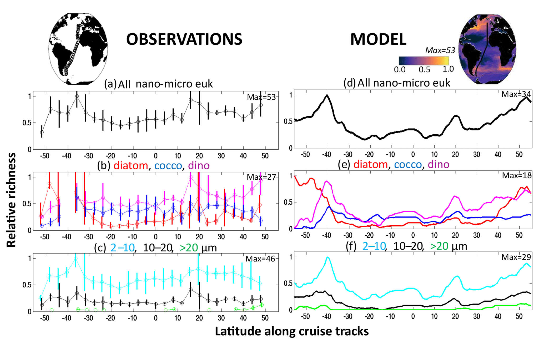
Figure 1Nano- and micro-eukaryote normalized richness in the Atlantic. Left: richness (number of coexisting species) normalized to the maximum along the Atlantic Meridional Transects (AMT) 1, 2, 3, 4 for microscopy counts (see methods). Right: normalized annual mean richness from model. (a, d) All diatoms, coccolithophores and dinoflagellates together; (b, e) each functional groups separately (red: diatoms, dark blue: coccolithophores, purple: dinoflagellates); (c, f) three size classes (light blue: 2–10 µm, black: 10–20 µm, green: <20 µm). In left panels, circles are means of the four transects (two in May, two in September) within 4∘ latitude bins; the vertical lines indicate the range within each bin. The maximum number used to normalize the plots is provided in each panel. Model pico-phytoplankton and diazotrophs are not included in the model analysis as they were not included in the observations. Maps show the cruise track of the AMTs, and the model includes the annual mean normalized richness of the diatoms, coccolithophores and dinoflagellates together.
2.2 Numerical model
The model follows from Dutkiewicz et al. (2015a) in terms of biogeochemistry, plankton interactions, and transmission of light as described by the tables and equations of that paper. However, the types of phytoplankton and zooplankton differ in that they include greater diversity. Here we briefly provide an overview of the model and detailed descriptions of the more complex ecosystem. More details of pertinent parameterizations and parameters can be found in Text S1, Figs. S1 and S2, and Tables S1 and S2 in the Supplement; the full set of equations and remainder of biogeochemical parameters can be found in Dutkiewicz et al. (2015a).
The biogeochemical/ecosystem model resolves the cycling of carbon, phosphorus, nitrogen silica, iron, and oxygen through inorganic, living, dissolved and particulate organic phases. The biogeochemical and biological tracers are transported and mixed by the MIT general circulation model (MITgcm, Marshall et al., 1997) constrained to be consistent with altimetric and hydrographic observations (the ECCO-GODAE state estimates, Wunsch and Heimbach, 2007). This three-dimensional configuration has a coarse resolution (1∘ × 1∘ horizontally) and 23 levels ranging from 10 m in the surface to 500 m at depth. At this horizontal resolution, the model does not capture mesoscale features such as eddies and sharp fronts, a limitation of the model that must be kept in mind when considering the results.
We use a complex marine ecosystem that incorporates 350 phytoplankton types that can be described in three “dimensions” of trait space (schematically shown in Fig. 2): size, biogeochemical function and temperature tolerance. Within the “size” dimension we include 16 size classes spaced uniformly in log space from 0.6 to 228 µm equivalent spherical diameter (ESD). Within the “biogeochemical function” dimension we resolve diatoms (that utilize silicic acid), coccolithophores (that calcify), mixotrophs (that photosynthesize and graze on other plankton), nitrogen-fixing cyanobacteria (diazotrophs) and pico-phytoplankton. We resolve 4 size classes of pico-phytoplankton (from 0.6 to 2 µm ESD), 5 size classes of coccolithophores and diazotrophs (from 3 to 15 µm ESD), 11 size classes of diatoms (3 to 155 µm ESD), and 10 mixotrophic dinoflagellates (from 7 to 228 µm ESD). Additionally, we resolve a “temperature norm” trait axis, where phytoplankton growth rates are defined over a specific range of temperatures (Fig. 3) by an empirically motivated function (e.g. Thomas et al., 2012; Boyd et al., 2013). We include 10 different norms. Thus for any size class within a functional group there are 10 different unique phytoplankton types (as demonstrated schematically in Fig. 2) with a different range of temperatures over which the cells will grow. Warmer-adapted types are assumed to grow faster as suggested empirically (Eppley, 1972; Bissenger et al., 2008) and from enzymatic kinetics (Kooijman, 2000). In total we resolve 350 phytoplankton types within 16 size classes, 5 biogeochemical functional groups, and 10 temperature norms.
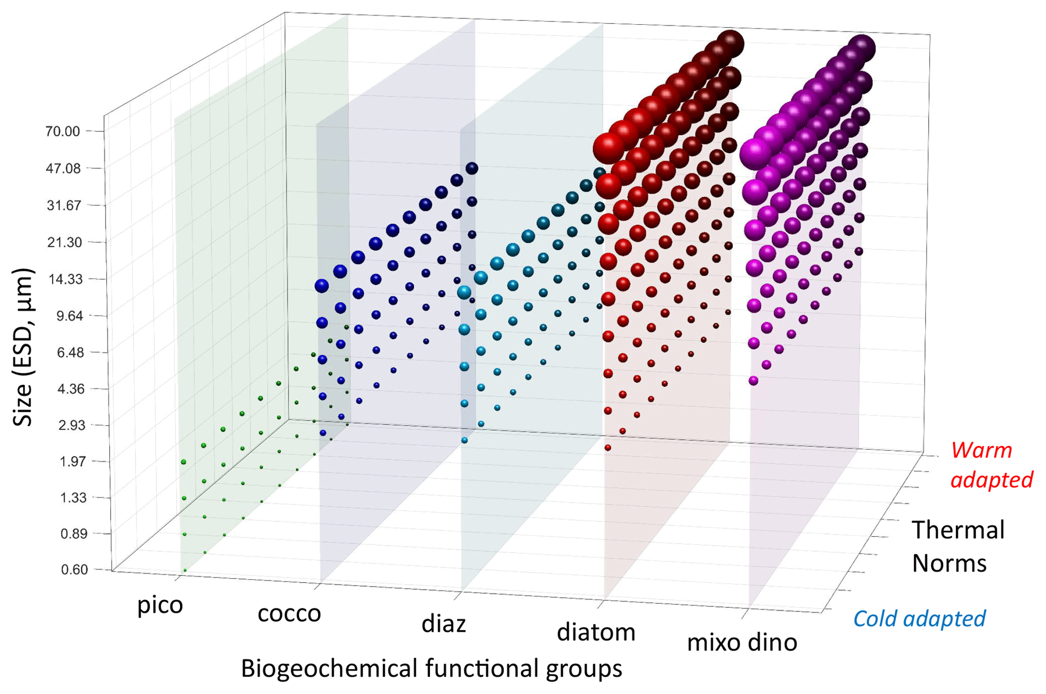
Figure 2Schematic of the three dimensions of trait space: size classes, biogeochemical functional groups and thermal norms. There are 16 size classes, 5 functional groups and 10 thermal norms. In all there are 350 individual phytoplankton types. However, the 3 largest size classes go extinct, and as such here (and in other figures) we show only 13 size classes.
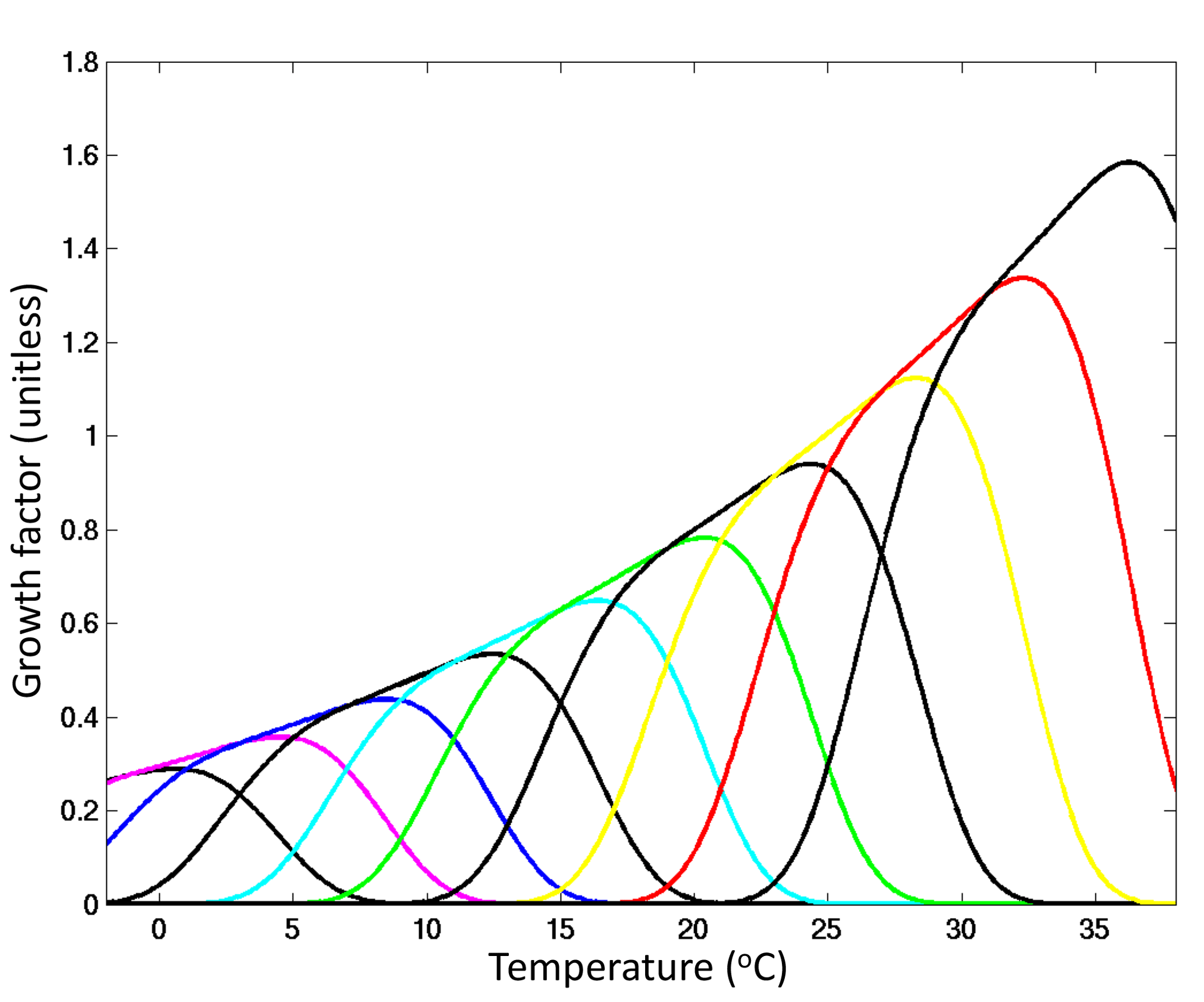
Figure 3Growth as a function of temperature. Shown are the 10 thermal norms (unitless), each with a different colour. The function used here is from Dutkiewicz et al. (2015b) and is discussed further in the Supplement.
Phytoplankton parameters influencing maximum growth rate, nutrient affinity, grazing and sinking are parameterized as a power function of cell volume: aVb (following Ward et al., 2012; see Text S1.2 and Table S2). Thus many size classes can be described by just two coefficients (a, b) per parameter. Maximum growth rate is parameterized (i.e. the a and b in the above equation) as distinct between functional groups (as suggested by observations in Fig. 4a; see also Buitenhuis et al., 2008; Sommer et al., 2017). The smallest diatoms (3 µm) have the highest maximum growth rates. Plankton smaller than 3 µm have an increase in growth rate with size, and those larger than 3 µm have a decrease in growth rate with size. This unimodal distribution has been observed (e.g. Raven, 1994; Bec et al., 2008; Finkel et al., 2010; Marañón et al., 2013; Sommer et al., 2017) and explained as a trade-off between replenishing cell quotas versus synthesizing new biomass (Verdy et al., 2009; Ward et al., 2017). There are also specific differences between functional groups in cell elemental stoichiometry and palatability to grazers (we assume that the hard coverings of diatoms and coccolithophores deter grazers; see e.g. Monteiro et al., 2016; Pančić et al., 2019). The smallest phytoplankton have the highest affinity for nutrients (Edwards et al., 2012) as a result of the lower surface-to-volume ratio found in larger cells (Kiorboe, 1993; Raven, 1994).
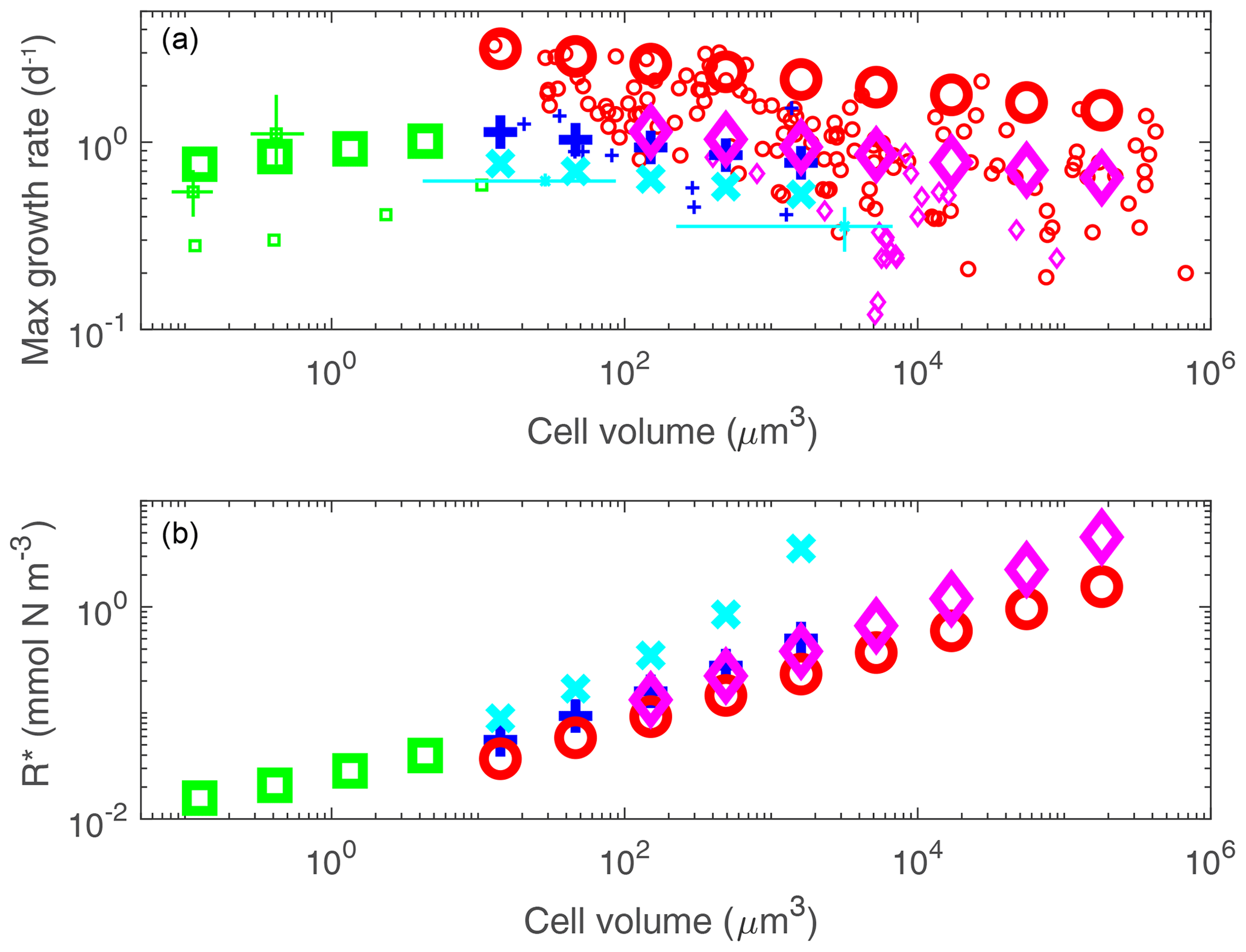
Figure 4Model parameter guide by laboratory studies. Phytoplankton maximum growth rate (a) and R* (b) as a function of cell size. In (a) small symbols indicate laboratory studies normalized to 20 ∘C and large symbols indicate the model size/functional groups. Colour of symbols denotes different functional groups: red circle, diatoms; purple diamond, mixotrophic dinoflagellates; dark blue plus, coccolithophores; light-blue cross, diazotrophs; green square, pico-phytoplankton. In (b), , where M=0.5 1 d−1 (see Appendix A). Data compilations of concurrent size and growth in (a) are from Tang (1995), Marañón et al. (2013), Sarthou et al. (2005) and Buitenhuis et al. (2008). Additional data are derived from separate measurement of size and growth: these are shown as light lines centred at the mean and arms covering range. These are for the pico-prokaryotes (green) Prochlorococcus and Synechococcus (Morel et al., 1993; Johnson et al., 2006; Christaki et al., 1999; Moore et al., 1998; Agawin and Agustí, 1997) and the diazotrophs (light blue) Crocosphaera and Trichodesmium (Garcia and Hutchins, 2014; Webb et al., 2009; Wilson et al., 2017; Bergman et al., 2013; Boatman et al., 2017; Breitbarth et al., 2008; Hutchins et al., 2007; Kranz et al., 2010; Shi et al., 2012).
The model includes spectral irradiances, and each functional group has different spectra for absorption (as a result of group-specific accessory pigments) and scattering of light. The absorption spectra are flatter with larger sizes following Finkel and Irwin (2000) to account for self-shading, and scattering spectra are also influenced by size following Stramski et al. (2001) (see Text S1.3, Fig. S1). The simulation uses Monod kinetics, and C : N : P : Fe stoichiometry is constant over time (though it differs between phytoplankton groups). Chl a for each phytoplankton type varies in time and space depending on light, nutrient and temperature conditions following Geider et al. (1998). Following empirical evidence, mixotrophic dinoflagellates are assumed to have lower maximum photosynthetic growth rates than other phytoplankton of the same size (Tang, 1995; Fig. 4a).
We resolve 16 size classes of zooplankton (from ESD 6.6 to 2425 µm) that graze on plankton (phyto- or zoo-) 5 to 20 times smaller than themselves, but preferentially 10 times smaller (Hansen et al., 1997; Kiorboe, 2008; Schartau et al., 2010). Maximum grazing rate is a function of size (following Hansen et al., 1997), though the four smallest grazers are assumed to have the same maximum grazing rates (Fig. S2). Here the smallest grazers do not have a clear difference in grazing related to size (following the data compilation of Taniguchi et al., 2014). Mixotrophic dinoflagellates also graze on plankton with the same predator–prey ratios as the zooplankton and have size-dependent maximum grazing rates. However, they have lower maximum grazing rates than zooplankton of the same size (Jeong et al., 2010, Fig. S2). We use a Holling III grazing function (Holling, 1959). Sensitivity studies with a Holling II parameterization show that the results here are not sensitive to this choice.
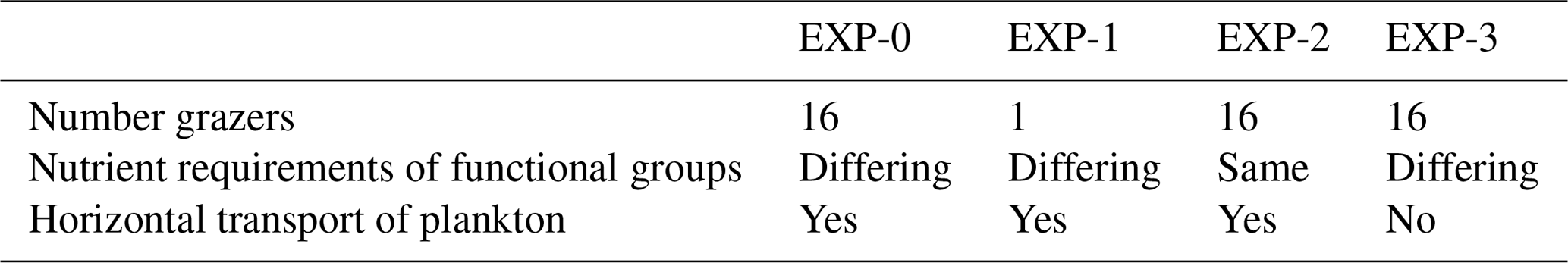
We perform a “default” simulation (EXP-0) for 10 years. The ecosystem quickly (within 2 years) reaches a quasi-steady state. Here we show results from the 5th year of the simulation but note that the patterns of biogeochemical and ecologically relevant output and diversity are not significantly different if we instead used the 10th year. We also conducted a series of sensitivity experiments, where we alter either physical or ecosystem assumptions to provide evidence for the controls of diversity (Table 1).
As mentioned in the introduction, in this study we primarily discuss diversity in term of “richness”, defined here as the number phytoplankton types that coexist at any location above a biomass threshold. We, in particular, look at the annual mean of the instantaneous surface richness (though see Supplement for examples with depth). Technically, we use a threshold value (10−5 mmol C m−3) to determine whether a phytoplankton type is present or absent in a given community. This value would convert to about 10 Prochlorococcus cells mL−1 (typical oligotrophic waters are above 103 cells mL−1), or only a tiny fraction (10−4) of a larger diatom cell per millilitre. Thus, this definition neglects rare species, often at abundances in the order of individuals per litre, that would be difficult to separate from numerical noise. This is why we do not account for the rare species in the AMT observations discussed above. The value of richness can be altered depending on the threshold chosen, but the patterns and results discussed below remain robust. We also emphasize that the level of richness that the model captures, though large for a model, is orders of magnitude lower than the real ocean. Thus, this is not a fully comprehensive study of diversity or species richness but does nevertheless provide a promising avenue for understanding some of the controls on diversity.
3.1 Diversity observations along the AMT
The four Atlantic Meridional Transect (AMT) cruises provide a large-scale consistent dataset of phytoplankton diversity including microscopic counts of diatoms, coccolithophores and dinoflagellates. Such microscopic measurements depict species richness patterns of abundant taxa but miss much of the rare biosphere. This dataset shows distinct large-scale patterns (Fig. 1a), with high richness (as determined by number of coexisting species) on the northern edge of the Southern Ocean and in the Canary upwelling, low richness in the subtropical gyres, and slightly elevated richness in the equatorial region.
However, the patterns of richness are very different if we look only within a single functional group (e.g. diatoms, Fig. 1b) or within a specific size class (Fig. 1c). Diatoms exhibit higher diversity in the Southern Ocean than the other functional groups, while the diversity of coccolithophores and dinoflagellates is much more uniform across the transects. Among size classes, the smallest size category (2–10 µm) has the highest diversity, while there is lower and more regionally varying diversity in the larger size categories, with some regions having none of the largest size class (>20 µm). This suggests that the controlling mechanism(s) on, for instance, diatom diversity is different to those controlling coccolithophore diversity, which also differs to what determines the diversity within different size classes. Indeed, modelling and theoretical work (e.g. Vallina et al., 2014b, 2017; Terseleer et al., 2014) have suggested that breaking diversity down into traits can be insightful. Thus, a starting point of our study is to separate out different dimensions of diversity.
3.2 Numerical model
Model development was guided by evaluating against a range of in situ and satellite-derived observations (see Text S2 and Figs. S3–S8). We refer the reader to the fuller evaluation in the Supplement text but provide a brief version here. The model captures the patterns of low and high Chl a seen in the satellite estimate (Fig. S4), though it underestimates the Chl a in the subtropical gyres and overestimates it in the high latitudes. However, we note that satellite-estimated Chl a has large uncertainties (Moore et al., 2009) especially in the Southern Ocean (e.g. Johnson et al., 2013). The coarse resolution of the model does not capture important physical processes near coastlines, and the lack of sedimentary and terrestrial supplies of nutrients and organic matter leads to Chl a being too low in these regions. The underestimation of Chl a in the gyres is also seen when comparing the model to the observations of surface Chl a along the AMT (Figs. 5b, S6b). The model does capture the drawdown of nutrients in the gyres and the large increase in nutrient concentrations in the Southern Ocean (Figs. 5a, S6a). However, the model overestimates the amount of silicic acid in this ocean (seen also in the global evaluation, Supplement Fig. S3), likely a reflection of Si : C of the model diatoms being too low in the region.
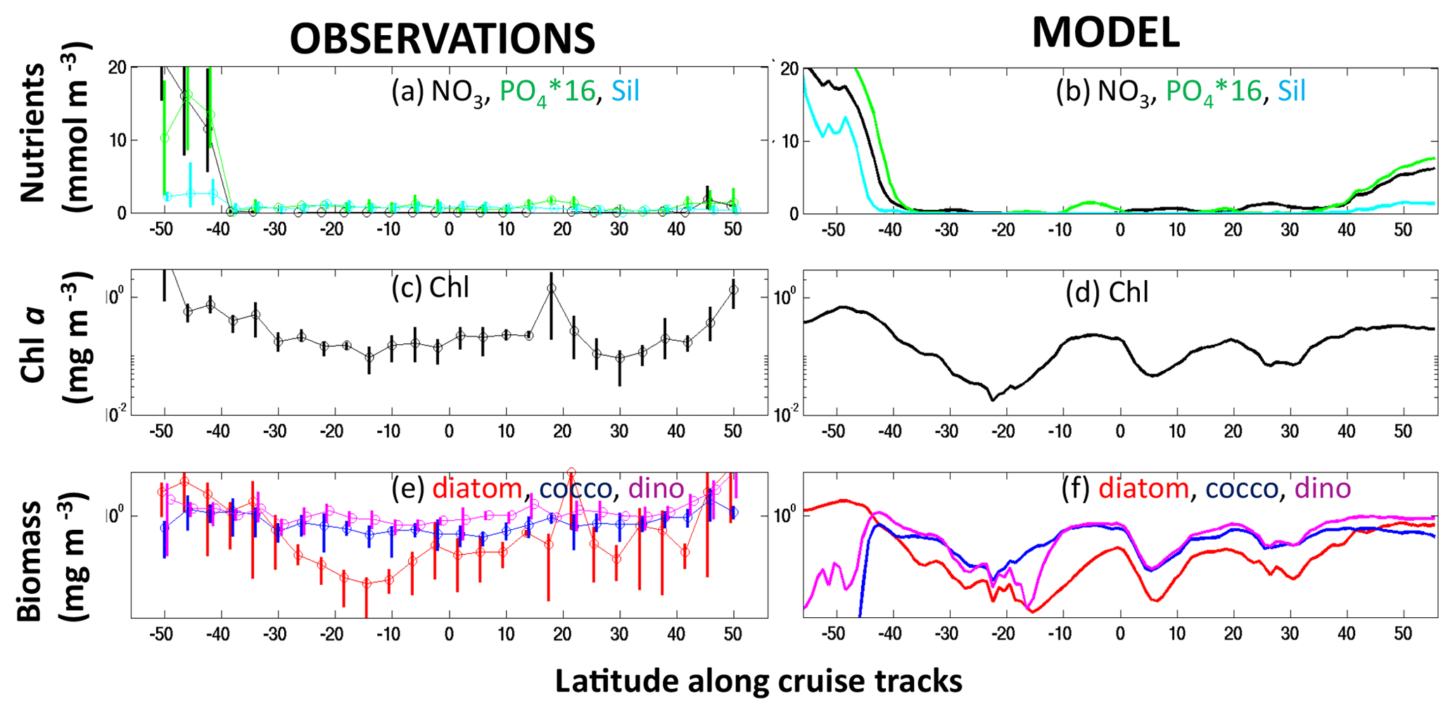
Figure 5Observations and model output along the Atlantic Meridional Transect (AMT). (a, b) Nutrients (black: nitrate, mmol N m−3; green: phosphate, ×16 mmol P m−3; light blue: silicic acid, mmol Si m−3); (c, d) Chl a (mg Chl m−3); (e, f) phytoplankton biomass (mg C m−3; red: diatoms; blue: coccolithophores; purple: dinoflagellates). Observations (left panels) are means (circles) for the four AMT cruises (two in May, two in September; see transects in Fig. 1 maps) in 4∘ bins; the vertical lines show the range within each bin. Model results are annual means along the AMT cruise track.
The model individual types have plausible ranges (four representative species shown in Fig. S9) compared to distributions determined from thermal niches (e.g. Thomas et al., 2012) and statistical techniques from sparse observations (e.g. Barton et al., 2016). The model captures biomass in almost all size classes (Figs. 6, S10a), though the largest size classes are underestimated. Traits not included in the model (e.g. buoyancy regulation, chain formation, symbiosis) are possibly more important for maintaining these large size classes. The model has biomass in all temperature norms (Figs. 6, S10c), though with lower biomass in the coldest- and warmest-adapted ones, suggesting the model parameterization covers an adequate range of norms. There are some interesting eliminations (which match observations) such as coldest-adapted smallest pico-phytoplankton and diazotrophs, as well as large warmest-adapted diatoms. The phytoplankton are complemented by a range of size classes of zooplankton (Fig. S11).
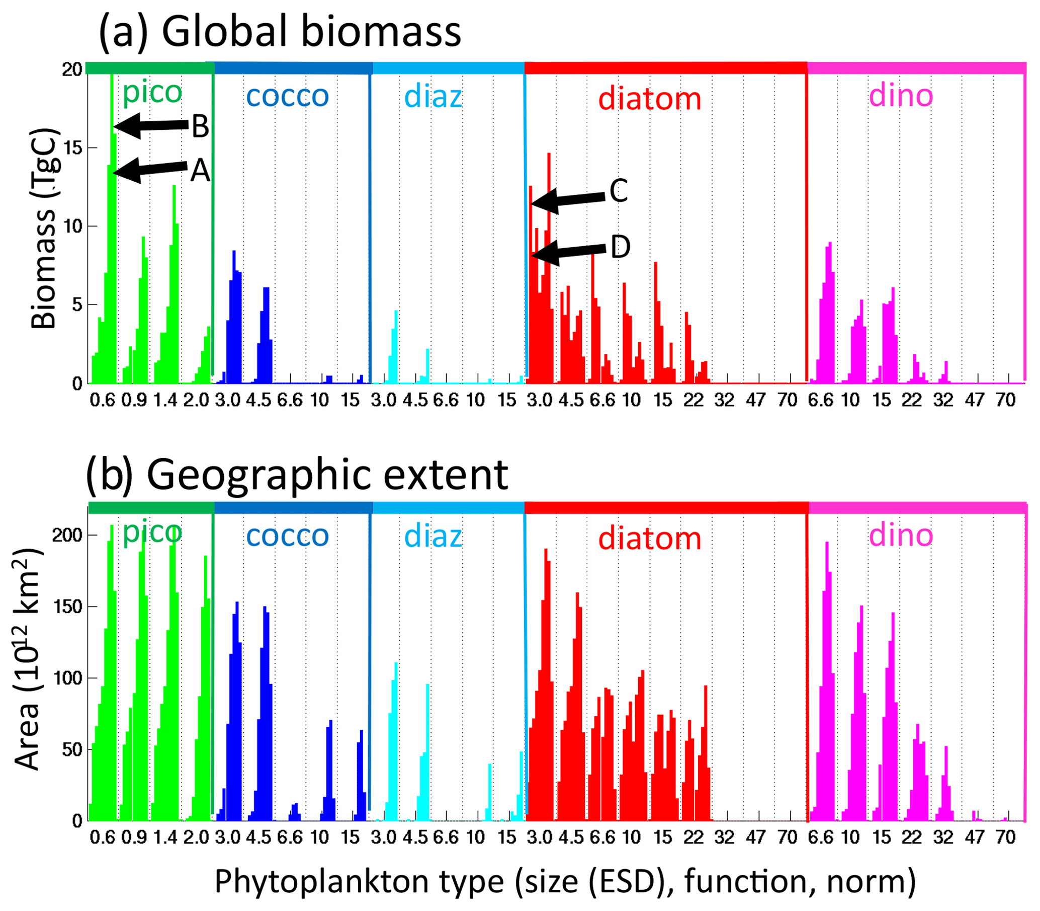
Figure 6Model phytoplankton types biomass and range. (a) Global integrated biomass (TgC); (b) areal extent of the type (1012 km2). Types are arranged by functional group as indicated by colour and labels at the top of the graph, by size classes (equivalent spherical diameter, ESD) as labelled below the graph, and by thermal norms from cold adapted to warm adapted from left to right in between vertical dotted lines. The text (A, B, C, D) in panel (a) refers to representative types whose distributions are shown in Fig. S9.
We evaluate the model's ability to capture the size distribution of phytoplankton as derived from satellite products (Figs. 7a, S4, S5). Here we capture the ubiquitous pico-phytoplankton and the limitation of the larger size classes to the more productive regions. The model pico-phytoplankton size class Chl a is potentially slightly too low and the nano size class too high. Though we note that if we set the pico/nano break at the fifth model size class (just under 3 µm) instead at the fourth (2 µm) size class, the relative values are much more in line with the satellite product. We suggest that the satellite product division might not be that exact. The micro-size class matches in location to the satellite product but is too low as discussed above.
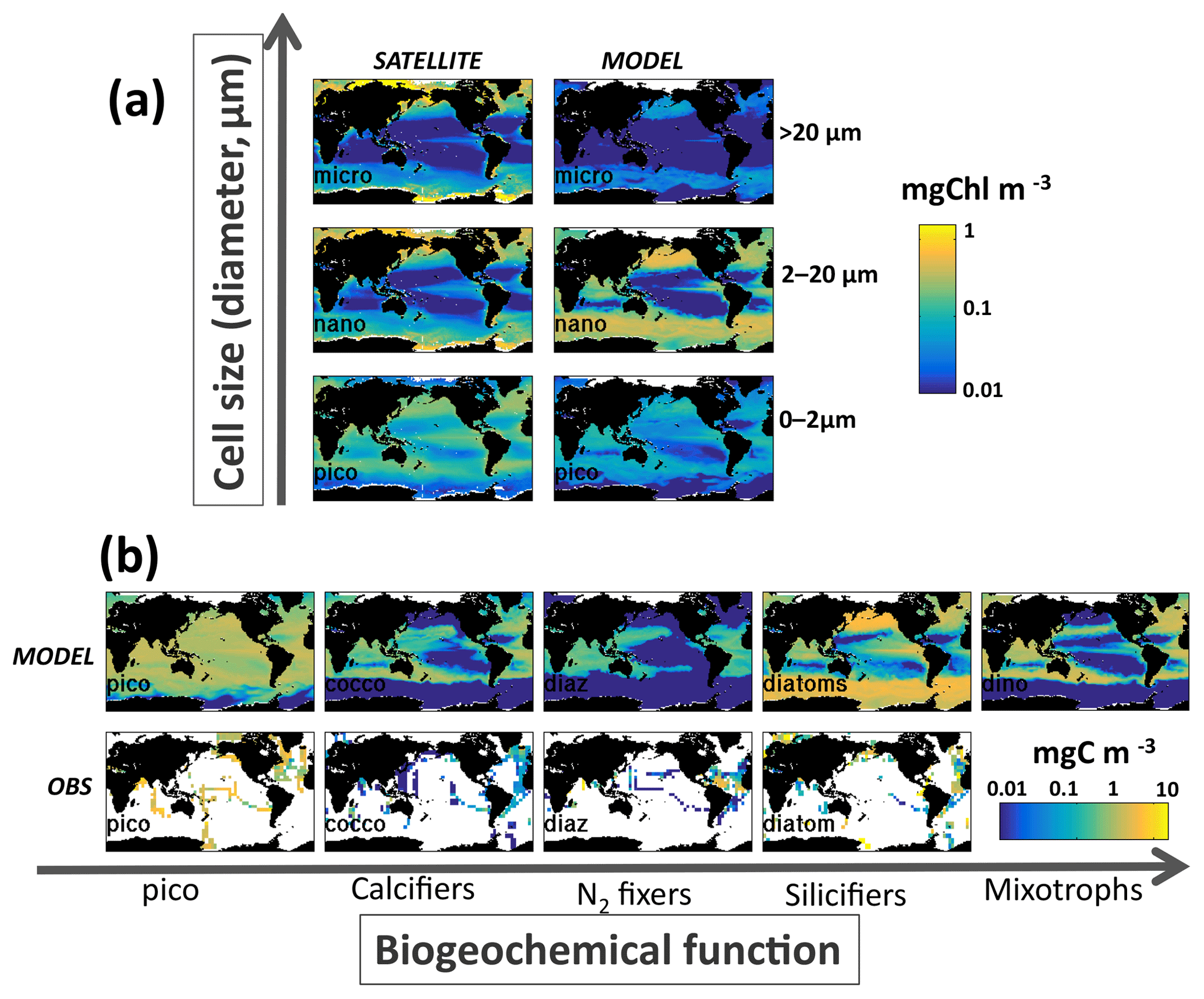
Figure 7Comparison to observations. (a) Sizes classes: Chl-a concentration (mg Chl m−3) in pico-phytoplankton (<2 µm), nano-phytoplankton (2–20 µm) and micro-phytoplankton (>20 µm) from (left) a satellite-derived estimate (Ward, 2015) and (right) default model (0–50 m); and (b) functional group (top) default model (0–50 m) and (bottom) data compilation (MAREDAT, Buitenhuis et al., 2013) in carbon biomass (mg C m−3). Note the difference in units for (a) and (b), chosen to match the appropriate observations. For the MAREDAT databases: pico-phytoplankton (Buitenhuis et al., 2012); coccolithophores (O'Brien et al., 2013); diazotrophs (Luo et al., 2012); diatoms (Leblanc et al., 2012). There was no MAREDAT dataset for dinoflagellates.
We also compare the model functional group distribution to the compilation of observations (Fig. 7b, MAREDAT, Buitenhuis et al., 2013, and references therein). Though the observations are sparse, we do capture the ubiquitous nature of the pico-phytoplankton, the limited domain of the diazotrophs (including the observed lack of diazotrophs in the South Pacific Gyre), and the pattern of enhanced diatom biomass in high latitudes and low in subtropical gyres. We overestimate the coccolithophore biomass relative to MAREDAT in many regions, but we note that the conversion from cells to biomass in that compilation was estimated to have uncertainties as much as several hundred percent (O'Brien et al., 2013). The MAREDAT compilation did not include a category for dinoflagellates. We also compare the model biomass of diatoms, coccolithophores and dinoflagellates along the AMT, though we note that the conversion from cell counts to biomass in the observations has significant uncertainties. The model captures the much lower biomass of diatoms in the subtropical gyres than the other two functional groups and higher biomass in the Southern Ocean. Coccolithophore biomass is too low in the Southern Ocean in the model, likely due to the modelled smallest diatom being parameterized as too competitively advantaged, but it compares better in the rest of the transect than the MAREDAT comparison above suggested.
In this study we mostly consider richness, the number of coexisting types, as a metric of diversity. However, we do discuss the Shannon index (another commonly used metric of diversity) later in the text. We will refer to “total richness”, i.e. the number of coexisting phytoplankton types, out of the 350 initialized in the model, at any location (Fig. 8a). Here we specifically look at the annual mean richness in the surface layer, which is a good indicator of the diversity within the mixed layer (Fig. S12). We find lowest richness in the subtropical gyres and highest associated with the western boundary currents.
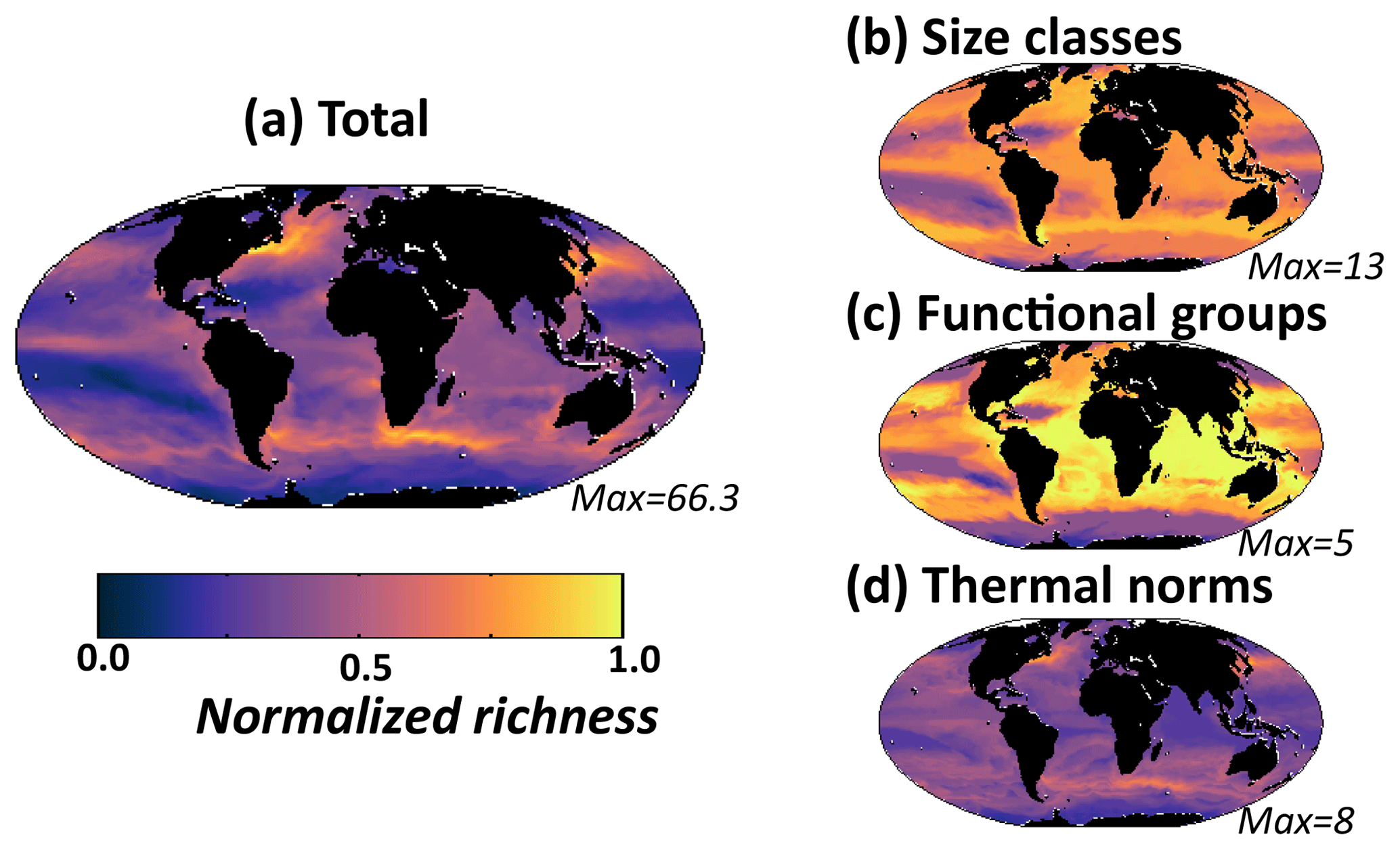
Figure 8Model diversity measured as annual mean normalized richness in the surface layer. Normalization is by the maximum value for that plot (value noted in the bottom right of each panel). (a) Total richness determined by number of individual phytoplankton types that coexist at any location; (b) size class richness determined by number of coexisting size classes; (c) functional richness determined by number of coexisting biogeochemical functional groups; (d) thermal richness determined by number of coexisting temperature norms. Total richness (a) is a (complex) multiplicative function of the three sub-richness categories (b–d). At first glance it may seem that thermal norm diversity (d) is most important, but this is only because our eyes are drawn to the hot spots. In reality, total diversity patterns (a) are strongly impacted by all three dimensions of diversity (see main text and sensitivity studies).
The model is designed to allow for richness within specific functional groups and size classes. A unique feature about this study is a comparison to the richness found in the AMT data (Figs. 1, S7, S8). The model captures the low and high patterns of the AMT observations, though it underestimates the diversity in the subtropical gyres. In these regions it is likely that trait axes (e.g. symbiosis and colony formation) not captured in the model provide additional means for phytoplankton to coexist. Excitingly the model also captures the differences in the diversity within functional groups and in size classes. Diatoms have much larger diversity in the Southern Ocean than the other functional groups, while coccolithophore and mixotrophic-dinoflagellate diversity is much more uniform across the transect. The model captures the much higher diversity within the smallest size category (2–10 µm) and the lower and much more regionally varying diversity in the larger size category, including the lack of diversity in the largest size class (>20 µm) in the subtropical gyres.
It is instructive to also consider richness along each of the dimensions of trait space. The number of size classes (irrespective of functional group or thermal norm) that coexist in any location will be referred to as size class diversity (Fig. 8b). We find that in high latitudes and along the Equator many size classes are present, while in the subtropical gyres only few small-sized classes survive (Figs. 7a, S10a). We find that there are different patterns of richness when looking along the two other axes of traits (Figs. 8c, d; S10b, c). Richness of biogeochemical functional groups is highest in the mid-latitudes, strongly linked to the distributions of diazotrophs (Figs. 7b, S10b). In contrast, the diversity within temperature norms is maximum in the western boundary currents, in particular the Gulf Stream and Kuroshio, and high in coastal upwelling regions (e.g. off Peru and Canary) and along the northern boundary of the Southern Ocean.
The total richness is a complex integral function (i.e. multiplicative) of the three different trait dimensions. At first glance total diversity (Fig. 8a) may look most like the thermal norm diversity (Fig. 8d), but this is mostly because our eyes are drawn to the hot spots. In reality, total diversity patterns are strongly impacted by all three dimensions of diversity as will be shown more clearly by the sensitivity experiments discussed later. We find that some trait dimensions are more (or less) important in different regions. For instance, thermal norm richness leads to the total richness hot spots (Fig. 8a) in the western boundary currents and coastal upwelling regions. While reduction in functional groups and thermal norms counteracts the increase in size classes in the Southern Ocean, all three dimensions together lead to the lowest total richness captured in the middle of the subtropical gyres.
None of these three dimensions can, in isolation, explain the controls on the total richness. Nor can we a priori understand the total richness. By using ecological theories and a series of sensitivity experiment (Table 1), we can begin to understand the mechanisms setting the different dimensions of diversity individually. Here, we step through each of the dimensions.
The theoretical frameworks are presented in Appendix A and are informed from the seminal work of Tilman (1977, 1982) and Armstrong (1994). Resource competition theory (Tilman, 1977, 1982) has been extensively used in theoretical and experimental studies (e.g. Sommer, 1986; Grover, 1991a, b; Huisman and Weissing, 1994; Schade et al., 2005; Miller et al., 2005; Wilson et al., 2007; Agawin et al., 2007; Snow et al., 2015) as well as in linking to numerical models (Dutkiewicz et al., 2009, 2012, 2014; Ward et al., 2013) to explain aspects of community structure. The theoretical underpinnings of size-selected grazing (Armstrong, 1994) have similarly been used in many studies (e.g. Lampert, 1997; Kiorboe, 1993, 2008; Schartau et al., 2010; Ward et al., 2014; Acevedo-Trejos et al., 2015). Appendix A and the insight we develop in the rest of this section are in some sense a synthesis of many prior studies. Here, these theories are specifically directed at understanding diversity patterns, something that to our knowledge has not been done before.
4.1 Size class diversity
We find that the richness of cell sizes increases with the supply rate of the limiting nutrient (Fig. 9). Theoretical predictions and previous model studies suggest that this should be the case when the resource requirements of phytoplankton increase with increasing size (Appendix A, Armstrong, 1994; Ward et al., 2014; Follows et al., 2018). In the nomenclature of resource supply theory (Tilman, 1977), R* of a phytoplankton type is the minimum resource concentration required for it to survive at a steady state. In the absence of grazing, , where KR is the resource half-saturation constant, μmax is the maximum growth rate and M is a loss rate (see Appendix A). The phytoplankton with the lowest R* will draw the nutrients down to this concentration and exclude all others. In our model, the smallest pico-phytoplankton have the lowest R* and larger phytoplankton have subsequent higher R* (Fig. 4b). In this formulation, the smallest phytoplankton should outcompete all others. However, when we take grazing by a zooplankton (Z) into account, , where g is a per biomass grazing rate. Thus, R* increases with increased grazing. When the grazing pressure is sufficiently strong on the smallest type, the R* of the next smallest phytoplankton is reached and the two phytoplankton can coexist. The smallest size class phytoplankton and its grazer have their biomass capped, and any increase in biomass is now due to the next size class (Armstrong, 1994). This process continues to more and more size classes as we go from regions of low to high nutrient supply rates (Fig. 9).
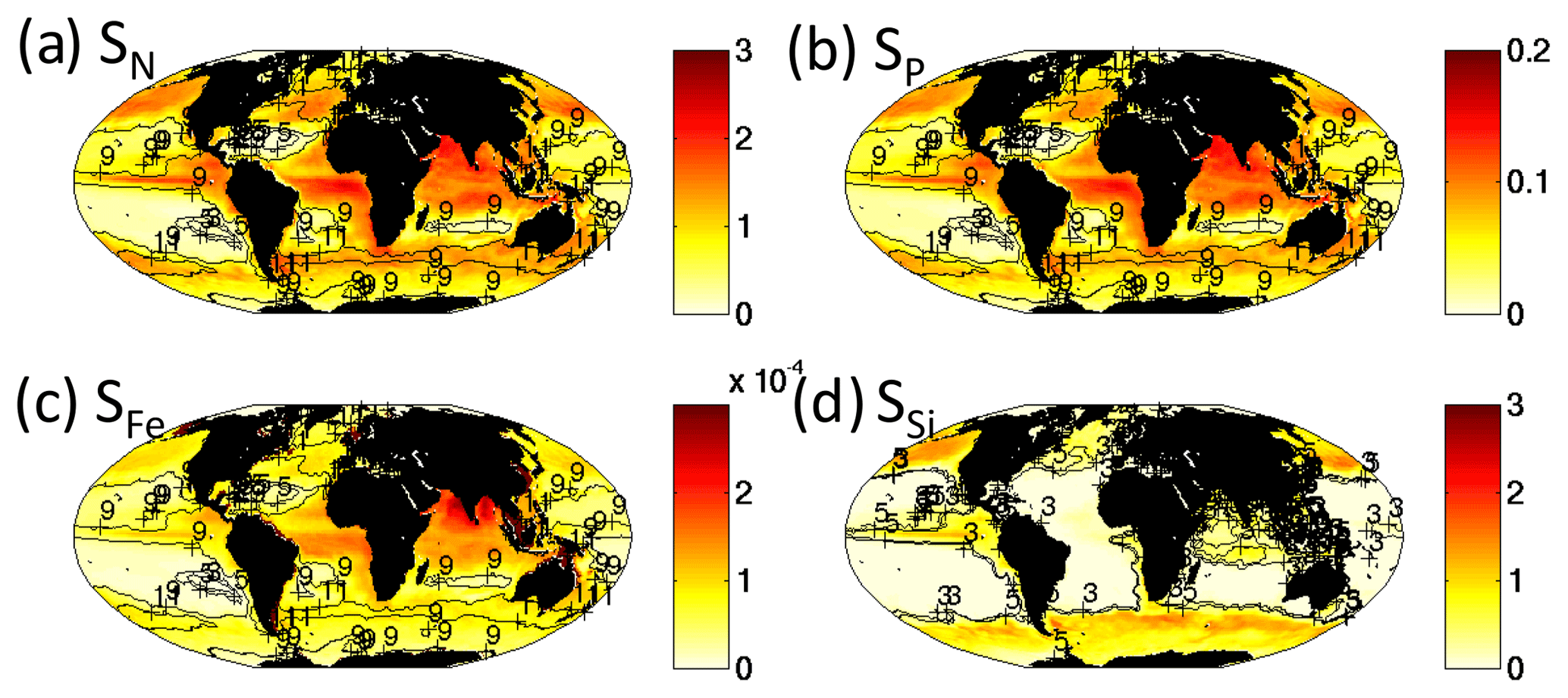
Figure 9Model rate of supply of nutrients into the top 50 m. Supply rate of (a) dissolved inorganic nitrogen (mol N m−2 yr−1), (b) phosphate (mol P m−2 yr−1), (c) iron (mol Fe m−2 yr−1) and (d) silicic acid (mol Si m−2 yr−1). All transport, diffusion and remineralization terms are included, and for iron dust supply is also included. In (a)–(c), contours are the size class richness from the total phytoplankton community (Fig. 4b), and in (d) the contour is for size classes within the diatom functional group alone. Since there are multiple limiting nutrients (especially for the non-diatoms), patterns of size diversity shown in (a)–(c) do not exactly match any single nutrient supply rate. However, the link between size classes of diatoms and silicic acid supply is clear in (d).
We note that the model is significantly more complex than the simple theoretical framework, including multiple limiting nutrients, multiple variants of one of those resources (NH4, NO2 and NO3) with differing affinities, additional loss terms (e.g. sinking), and more complicated grazing and food web (rather than food chain). However, this framework still helps us understand the patterns of size diversity in the model.
In the model, some regions have different limiting nutrients (e.g. iron versus dissolved inorganic nitrogen), so the patterns of size diversity from the total community are more complicated than considering only one nutrient supply rate. However, this process is nicely shown by the number of size classes within the diatom group alone increasing cleanly with the supply of silicic acid (Fig. 9d). The fact that each size class is capped by grazing leads the distributions of size classes to be relatively even, especially in the highest nutrient regimes (shown by the Shannon index, Text S3, Fig. S13).
To explore the importance of size-specific top-down control on diversity suggested by this theoretical construct, we conduct a sensitivity experiment (EXP-1, Table 1), where we allow only one grazer to prey on all phytoplankton. We also do not allow for mixotrophy. We find that only the smallest size class in each functional group survives (Figs. 10b, S14): the 0.6 µm pico-phytoplankton and the 3 µm diazotrophs, coccolithophores and diatoms. The dinoflagellates do not survive without mixotrophy. The size diversity reduces to one in most regions (Fig. 11). This experiment highlights that size diversity (Fig. 8b) is controlled not only by the rate of supply of the limiting nutrients, but also by size-specific grazing (Armstrong, 1994; Poulin and Franks, 2010; Ward et al., 2012).
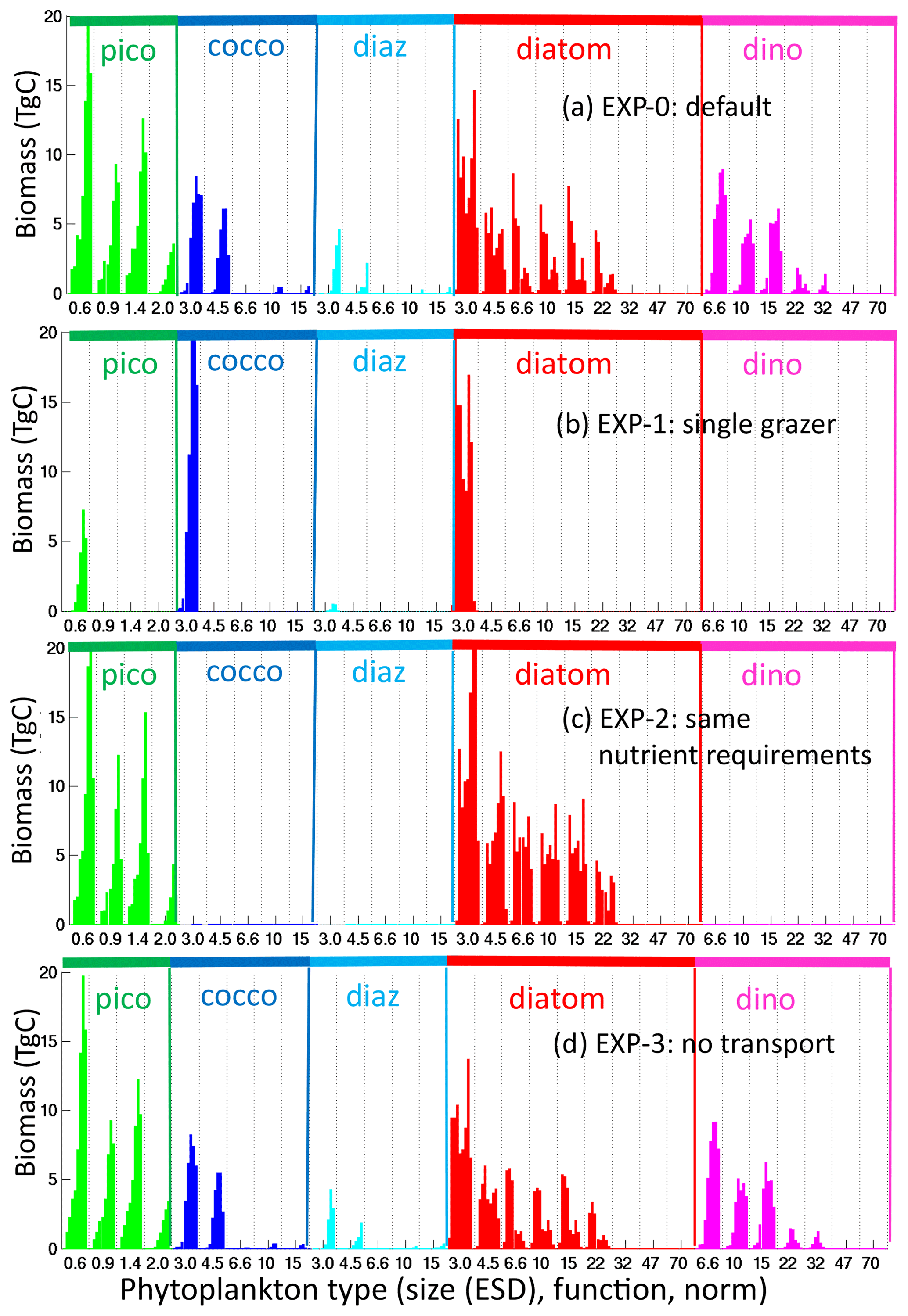
Figure 10Sensitivity experiments: phytoplankton global biomass. Global integrated biomass (TgC) for (a) default experiment (identical to Fig. 6a); (b) EXP-1 (experiment with single generalist grazer); (c) EXP-2 (experiment where all phytoplankton have same nutrient requirements); (d) EXP-3 (experiment where plankton are not transported). Types are arranged by functional group as indicated by the colour and labels at the top of the graph, by size classes (equivalent spherical diameter, ESD) as labelled below the graph, and by thermal norms from cold adapted to warm adapted from left to right in between vertical dotted lines.
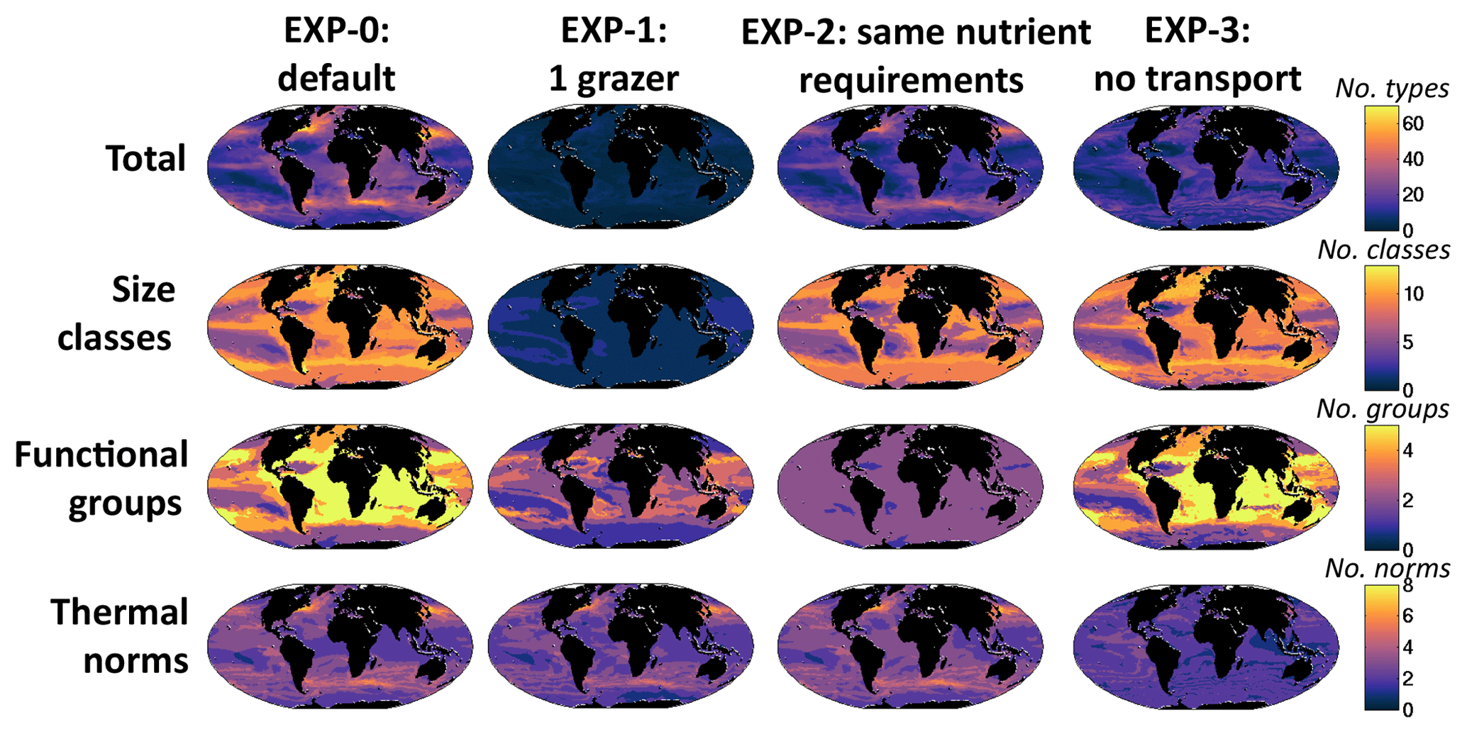
Figure 11Sensitivity simulations: model annual mean richness. EXP-1 has no size-dependent loss rates (i.e. only one grazer); EXP-2 has no nutrient requirement differences between functional groups; EXP-3 has no transport of the plankton (all nutrients and non-living organic pools are transported). Top row: total richness; second row: size class richness determined by number of coexisting size classes; third row: functional richness determined by number of coexisting biogeochemical functional groups; bottom row: thermal richness determined by number of coexisting temperature norms. The leftmost column is the same output as shown in Fig. 8a, b, c, d for the original (“default”) experiment, but with absolute values (i.e. not normalized).
The thermal norm richness of EXP-1 is very similar to the original default experiment (Fig. 8d), and thus richness of this dimension is not (at least greatly) controlled by size-specific grazing. Functional group richness decreases as the dinoflagellates are no longer viable without mixotrophy. All other functional groups survive (Figs. 10b, S14), and there is coexistence at the functional level; however, the patterns are different to the default experiment. In EXP-1 there are significant changes to the biogeochemistry, including the primary production (lower) and subsequent changes to nutrient supplies. It is these biogeochemical changes that alter the functional richness patterns (discussed more below). However, the total diversity reduces dramatically (Fig. 11, top row). Patterns of hot spots are, however, still apparent, but the increases in diversity with higher nutrient supply are no longer apparent.
We have used steady-state theory to explain the coexistence of size classes. We contend that when looking at annual average richness this theory provides insight even in non-steady-state regions such as the highly seasonal latitudes. However, we do acknowledge that the processes are more complex in these regions. For instance, during times of resource-saturated conditions (e.g. beginning of the spring blooms), the smallest diatoms, which are the fastest-growing phytoplankton, will dominate (Dutkiewicz et al., 2009; see Appendix A). However, as the grazer of the smallest diatom increases, the phytoplankton net growth rate (growth minuses losses) decreases until the next fastest-growing phytoplankton (whose net growth rate is higher since it is not yet under grazer control) is able to grow in (Fig. 12). Such a progression of size classes of diatoms has been observed using Continuous Plankton Recorder (CPR) data (Barton et al., 2013) and modelled for a coastal system (Terseleer et al., 2014). This process of succession continues until nutrients are drawn down, allowing the pico-phytoplankton and mixotrophs to dominate in this more-steady-state lower-nutrient environment (as suggested by Margalef's mandala, Margalef, 1978). Given that annually there is an optimum condition for each of those size classes, they do all coexist though at seasonally varying abundances (i.e. they never go extinct locally).
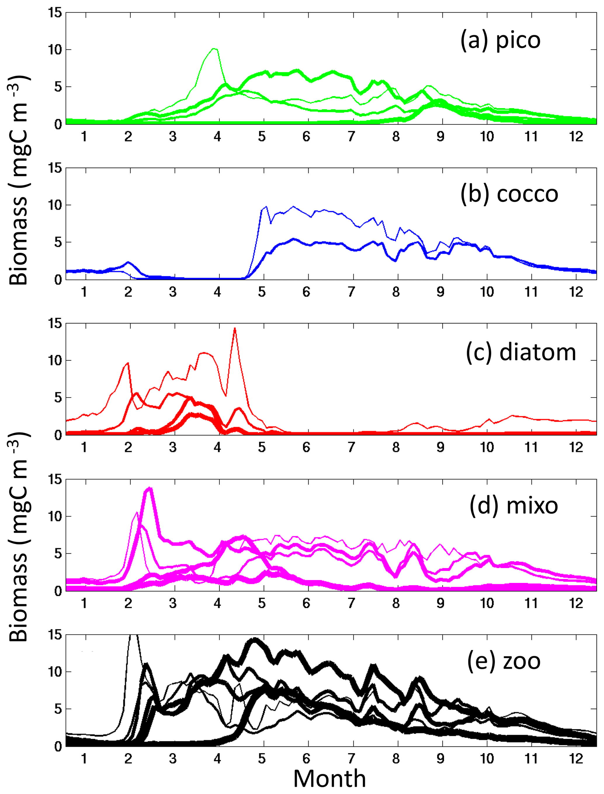
Figure 12Default model time series in the North Atlantic (20∘ W, 45∘ N). Carbon biomass (mg m−3) of (a) pico-phytoplankton functional group binned by size class; (b) coccolithophores binned by size class; (c) diatoms binned by size class; (d) mixotrophic dinoflagellates binned by size class; (e) zooplankton binned by size class. Diazotrophs do not survive at this location. The line width goes from thinnest for the smallest size class of each phytoplankton functional group and gets thicker for each larger size class (i.e. thinnest line is for 0.6 µm picophytoplankton, 3 µm for diatoms, etc.). For the zooplankton, however, the thickness of the line is linked to the preferential diatom prey size (i.e. 30 µm ESD zooplankton for the thinnest line), to show the zooplankton–diatom interactions.
4.2 Functional group diversity
The size class and functional group classifications are not completely orthogonal as the “pico-phytoplankton” group is entirely composed of the four smallest size classes. We therefore use a similar explanation as to why pico-phytoplankton can coexist with the other functional types in low seasonality regions: the low R* of pico-phytoplankton allows them to survive ubiquitously and other functional groups can only coexist where (or when) grazing pressures on the pico-phytoplankton and resource supplies are high enough.
We find that for the rest of the functional groups, coexistence is strongly controlled by the differences in their resource requirements and the imbalances in the supply rates of multiple resources (resource supply ratio theory, Tilman, 1982; see Appendix A). For instance, slow-growing diazotrophs can only coexist with faster-growing phytoplankton groups when there is an excess supply of iron and phosphorus delivered relative to the non-diazotroph N : P and N : Fe demands (Fig. 13a, b, c; Dutkiewicz et al., 2012, 2014; Ward et al., 2013; Follows et al., 2018). In such locations, the non-diazotrophs are nitrogen limited, while the diazotrophs can fix their own nitrogen, and the excess P and Fe not utilized by the non-diazotrophs is available (Appendix A; Fig. 13b, c).
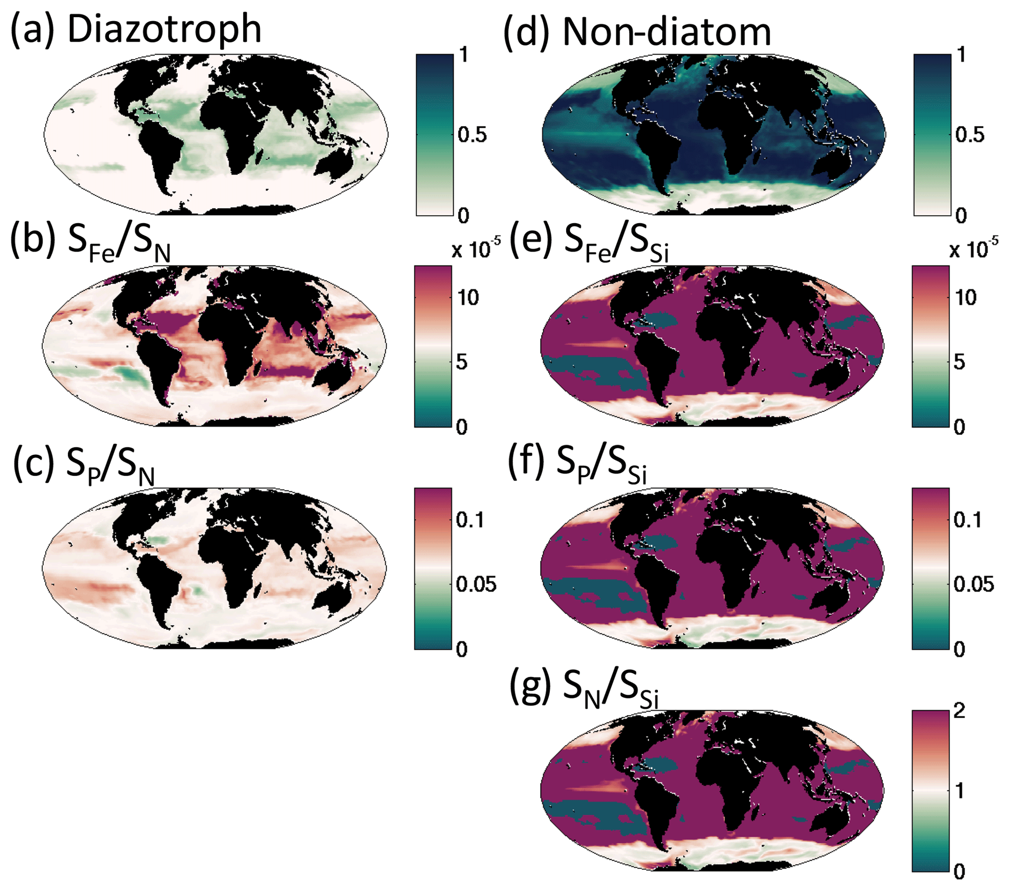
Figure 13Coexistence of functional types defined by imbalance of different nutrient supply rates. Left column depicts controls on diazotroph distribution: (a) fraction of total biomass made up of diazotrophs; (b) ratio of iron to dissolved inorganic nitrogen (DIN) supply rates (see Fig. 9); (c) ratio of phosphate to DIN supply rate. Colour scale is chosen such that purple indicates supply rate ratios in excess of the non-diazotroph Fe : N and P : N requirements. Right column depicts the controls on the coexistence of diatoms and non-diatoms: (d) fraction of biomass made up of non-diatoms; (e) ratio of iron to silicic acid supply rates; (f) ratio of phosphate to silicic acid supply rate; (g) ratio of DIN to silicic acid supply rates. Colour scale is chosen such that purple indicates supply rate ratios in excess of the diatom Fe : Si, P : Si and N : Si requirements.
Similar arguments explain where non-diatoms can coexist with the fast-growing diatoms (Fig. 13d). In regions where there is excess supply of dissolved inorganic nitrogen, phosphate, and iron relative to the diatom Si : N, Si : Fe, and Si : P demands, there can be coexistence (Fig. 13e, f, g). In these locations (or occasions), diatoms are limited by silicic acid, and any excess N, P and Fe can be used by the other phytoplankton. When the excess supply is significantly high, non-diatoms can dominate. The high silicic acid supply in the Southern Ocean leads to lower diversity as the diatoms win out in all but the low-nutrient summer months, when (in this simulation) pico-phytoplankton are the only other functional group to survive. In other seasonal regions, such as the northern North Atlantic (Fig. 12), diatoms dominate at the beginning of spring, but coccolithophores can outcompete later in the summer when the diatoms become limited by availability of silicic acid.
The mixotrophs have two sources of resources: inorganic nutrients and other plankton. They are parameterized to photosynthesize slower than other phytoplankton (of the same size, as suggested by observations, Tang, 1994; Fig. 4a) and graze slower than other grazers (of the same size, Jeong et al., 2010; Fig. S2). They are advantaged over specialist autotrophs and heterotrophs when competition for both inorganic nutrients and prey is strong, and, by using both, their R* for each resource is lowered.
To demonstrate that differential nutrient requirements lead to much of the functional group coexistence, we conduct another sensitivity experiment (EXP-2, Table 1) where we force all functional groups to have the same resource requirements (e.g. diatoms do not require silicic acid, diazotrophs cannot fix nitrogen, dinoflagellates cannot graze on other phytoplankton) and C : N : P : Fe ratios are the same for all types. All other growth and grazing parameterizations remain the same as in the default experiment. In EXP-2, the functional richness reduces dramatically (Fig. 11), and only pico-phytoplankton and diatoms survive (Figs. 10c, S15). The diatoms are the ultimate opportunists (r-strategists) in this model, with the highest growth rate (Fig. 4a), and survive when nutrient supplies are high enough. Without any differentiating nutrient requirements relative to the other functional groups, they outcompete them. Pico-phytoplankton (the gleaners, k-strategists) survive in regions of lowest nutrient supply, where their low R* and low grazing allows them to exclude the diatoms. Size class and thermal norm diversity change very little (Fig. 11). Total diversity is reduced everywhere but mostly in the lower latitudes where the loss of diazotrophs and coccolithophores has a high impact.
4.3 Thermal norm diversity
We find that thermal norm richness is highest in the regions of the western boundary currents and other regions generally anticipated to have high levels of mixing of different water masses. Clayton et al. (2013) identified a link between hot spots of diversity and eddy kinetic energy and the variance in sea surface temperature. Anticipating the role of currents and mixing of water mass (Clayton et al., 2013; Lévy et al., 2014), in a third sensitivity experiment (EXP-3, Table 1) we do not allow transport of plankton between grid cells, though we do allow diffusion vertically in the water column. Thus, this simulation is a collection of one-dimensional models with regard to the plankton. However, nutrients and dissolved and detrital organic matter are allowed to be transported as in the default experiment. Thermal norm diversity decreases (Fig. 11), and there are no longer hot spots. These results echo findings from Lévy et al. (2014) and clearly show the importance of mixing of water masses for maintaining thermal norm diversity. When temperature is fluctuating, all phytoplankton with different temperature norms can survive together provided their respective temperature optimal occurs for long enough (Kremer and Klausmeier, 2017) or there is a constant supply of the types from upstream (Clayton et al., 2013). This is different from resources or grazing control where competition for limited resources is the main process controlling coexistence (or lack thereof), and as such we find the greatest effect in EXP-3 on thermal norm diversity. Total diversity is reduced everywhere but most dramatically in these hot-spot regions. Both Clayton et al. (2013) and Lévy et al. (2014) showed the importance of eddies in enhancing this process of transport-mediated diversity. Thus the hot spots in the default experiment would likely be even higher in a model that did resolve the mesoscale.
We find in EXP-3 that the geographical size of almost all habitats (Figs. 14, S16) is reduced. In the case of thermal norms, the lack of transport allows for very little coexistence. For functional diversity, the pattern changes, but the maximum richness remains the same. This suggests that the boundaries of functional group domains are expanded by transport (see for instance the decrease expanse of diatoms in the gyres, Figs. S16 versus S10), but transport per se is not the ultimate controller. Domains for each size class also decrease (Figs. 14, S16), but most dramatically for the larger size classes, and the two largest go extinct in this experiment. This suggests that transport also plays a role in maintaining the grazer/phytoplankton links and that for classes with smaller domains and/or very low biomass this becomes more crucial. A few types have an increase in range or in fact exist in EXP-3 and not in the original experiment (Figs. 10d, 14, S16). These are almost all the warmest-adapted types that in EXP-3 have very small biomass and ranges. Thus, transport can also reduce domains of types with very small potential niches as the constant influx of less-fit types from cooler regions is sufficient to overcome any competitive advantage of the locally superior warm-adapted types (see Appendix A).
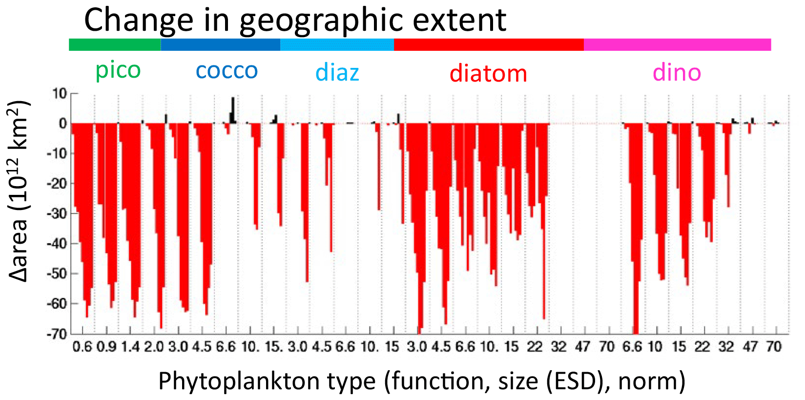
Figure 14EXP-3 difference in phytoplankton range geographic extent. Change in areal extent of all phytoplankton types (1012 km2) between EXP-0 and EXP-3 (no horizontal transport of plankton). Negative (red) indicates a decrease in the geographic domain of the phytoplankton type. Types are arranged by functional group as indicated by the coloured labels at the top of the graph, by size classes (equivalent spherical diameter, ESD) as labelled below the graph and by thermal norms from cold adapted to warm adapted from left to right in between each vertical dotted line. Differences are relative to those shown in Fig. 6b.
Using the results of this study, we can hypothesize as to why richness of coexisting nano- and micro-eukaryotes along the AMT (Figs. 1a, 15a) has the observed patterns. We consider the modelled diversity within the three dimensions along the transect (Fig. 15b, c, d). All three dimensions have high diversity along the northern edge of the Southern Ocean (labelled A in Fig. 15), suggesting that all controls (supply rate of limiting nutrient, imbalance in the supply of different nutrients, top-down control and transport) are at play in setting the maximum richness seen here in both the model and observations (Fig. 1a, d). Thermal and functional richness decrease southward, leading to the drop in total richness observed poleward. Absolute nutrient supplies are still high enough to maintain size diversity, but the N : Si supply ratios are no longer conducive to maintaining coccolithophores (Fig. 13e, f, g), and their diversity decreases as is observed (Fig. 1b, e). In this southernmost region there is also no longer the mixing of different water masses between the subtropical and Southern Ocean to promote large thermal norm diversity. However, diatom diversity (due here to size classes) increases (Fig. 1b, e), driven by the large gradient in silicic acid supply rate (Fig. 9d).
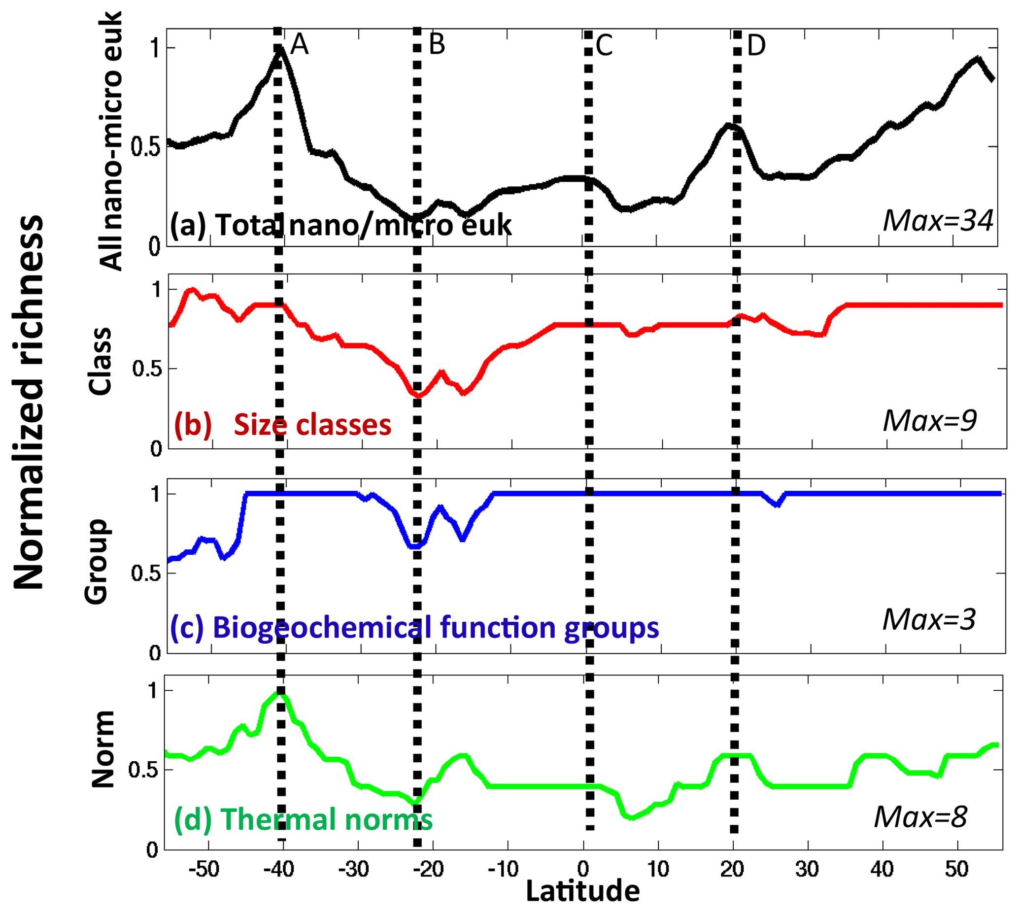
Figure 15Modelled nano- and micro-eukaryote normalized richness along the Atlantic transect. Annual mean richness normalized to the maximum in a transect similar to AMT for (a) all diatoms, coccolithophores and dinoflagellates – this panel is the same as Fig. 1b; (b) size classes; (c) biogeochemical functional groups; and (d) thermal norms. The normalization factor is given on the bottom right of each panel. Note that pico-phytoplankton and diazotrophs are not included in this analysis as they were not part of the observations. Dashed lines and text (A, B, C, D) are used to locate regions discussed in the text.
All three dimensions have an even sharper decrease equatorward of the Southern Ocean boundary, leading to much lower total diversity observed in the South Atlantic subtropical gyre (labelled B in Fig. 15). Here the lower absolute nutrient supply likely leads to a reduction in size classes, silicic acid supply rates drop dramatically (Fig. 9d) and functional diversity decreases. The lack of mixing of water masses reduces the thermal norm diversity. Nearer the Equator (labelled C), both size and functional diversity are high, leading to the observed increase in total diversity. Here an increased supply of nutrients (Fig. 9) from equatorial upwelling, including slightly higher Si supply rates, is probably important for allowing additional size classes and diatoms to exist. In the region of the Canary upwelling region (labelled D), there is an increase in diversity in the model and observations. Here increased size class and thermal norm diversity are possibly responsible, a result of the nutrient-rich upwelled water mixing with surrounding water masses as it is transported offshore (see Clayton et al., 2013). The model underestimates this increase since the model's coarse resolution does not capture the mesoscale filaments associated with these upwelling features found in the real ocean.
This study must be understood within the context of the limitations of the model. Models are by definition simplified constructs that attempt to capture the essence of a real system. The model here has a more complex ecosystem than many other marine models but is still limited in terms of the parameterization choices. For instance, the size-dependent grazing assumes a 10-to-1 preference as suggested by observations and used in many other studies (Fenchel, 1987; Kiorboe, 2008; Ward et al., 2012; Baird et al., 2004). However, there are many examples of grazing that break these preference rules (Jeong et al., 2010; Weisse et al., 2016; Sommer et al., 2018). The model assumes fixed elemental ratios in the plankton. This too is an oversimplification, and variable ability to store nutrients and modify cellular quotas is an important trait that likely allows for levels of coexistence (Edwards et al., 2011). This level of stoichiometric complexity is not incorporated here. However, the model carries almost 750 unique tracers to account for all the phytoplankton, variable Chl a, and the inorganic and organic pools. To include variable stoichiometry would add over 2000 more tracers, which is computationally unfeasible for this study. Each functional group has a different absorption spectrum, though these are modified with size (see Text S1.3 and Fig. S1); we recognize that this has a large implication for the pico-phytoplankton whose accessory pigments are quite different. Using a version of this model, but with differing absorption spectra for the pico-phytoplankton, Hickman et al. (2010) showed that such a difference was responsible for some niche separation, especially vertically. The results of this study should be interpreted in light of these and other simplifications.
The model considers only three axes of phytoplankton traits. We anticipate that additional axes such as morphology (e.g. shape, spines), motility (e.g. flagella), chains and colony formation, nutrient storage abilities, and symbiosis will each have their own controlling mechanisms. Such traits might allow the model to capture more species and, particularly, more large-sized phytoplankton types. Previous studies have suggested other controllers of phytoplankton distributions when considering other traits, for instance the importance of trade-offs between nutrient acquisition and storage (e.g. Edwards et al., 2011) or the effect of symbioses (e.g. Follett et al., 2018; Tréguer et al., 2017). Here, we have specifically designed the model to only consider the three dimensions for simplicity. Including additional trait dimensions will likely lead to alterations to the patterns of diversity and will be important for follow-on studies, especially as our knowledge of the trade-offs of each trait dimension becomes clearer. For instance, the fact that the model underestimates diversity in the subtropical gyres suggests that additional dimensions are likely important in these regions.
Our results are also dependent on the resolution of different axes of trait space. Likely in the real ocean there is a similar (though more complex) coarse resolution of functional groups but much higher (potentially continuous) resolution of size classes and thermal norms. Total diversity may therefore be influenced more by these two axes than established in this study. Our model only captures a tiny (probably orders of magnitude less) amount of the diversity found in the real ocean. Including more resolution along these axes and including additional trait axes would allow for further diversity but is beyond the scope of our study. This study should be viewed as only a step in the understanding of controls of diversity and provides new evidence to explain the “paradox of the plankton” (Hutchinson, 1961). However, that we can capture the major patterns of the AMT (Figs. 1, S7) suggests that we have included some of the most important mechanisms.
Given computational constraints with this complexity of ecosystem model, we have used a coarse-resolution physical model that does not capture explicit meso- or subscale features. Previous studies (e.g. Clayton et al., 2013; Lévy et al., 2014) have shown the importance of such features in modulating diversity. Meso- and sub-mesoscale features give rise to temporal increases in nutrient supplies (see e.g. Clayton et al., 2017), and, according to our results, this suggests temporal increases in size classes during such events. Sub- and mesoscale mixing in frontal regions will also enhance species richness in hot spots (Clayton et al., 2013) but also result in a general increase in species richness (Lévy et al., 2014).
We have used ecological theories and a numerical model to examine the controls on phytoplankton diversity along a number of trait dimensions. We find that each dimension has a different set of controls. Observed total diversity is an integrated function of the richness along each trait dimension and is thus controlled by many different mechanisms. By focusing on the mechanisms, we can understand the patterns of diversity at the fundamental level. Such insight provides us with a perspective to predict changes that might occur in diversity in, for instance, a warming world.
Our results suggest that observed patterns of total diversity (or for any grouping of phytoplankton types, such as for nano- and micro-eukaryotes along the AMT) are a result of multiple controllers: supply rate of limiting resource; imbalance in the supply of different resources relative to competitors' demands; top-down control, particularly in terms of size-dependent grazing; and transport processes. The importance of both resource supply and resource imbalance (or resource supply ratio) has previously been demonstrated by Cardinale et al. (2009) for lake habitats and more recently for other natural phytoplankton assemblages (Lewandowska et al., 2016).
In this study we have synthesized the previously known theory and a numerical model. The results explain why previous model results have had sometimes contradictory results. In ecosystem models that only considered two dimensions of diversity (functional groups and thermal norms, Barton et al., 2010; Clayton et al., 2013), different patterns where obtained relative to a model that only considered size (Ward et al., 2014). For instance, the hot spots of diversity in western boundary currents were not apparent in the study of Ward et al. (2014) since thermal norm diversity was not included in that study. Similarly, the lack of high diversity along the edge of the Southern Ocean in Barton et al. (2010), seen in this study and in the AMT observations (Fig. 1), was due to the lack of a size trait dimension in that study. This stresses that diversity in models needs to be understood in terms of the traits that are included. This obviously bring up the questions raised in Sect. 6: what additional patterns will be apparent in models that include additional, or other, trait dimensions? This is an exciting avenue for future study.
The drivers we found in this study (supply rate of limiting resource, imbalance in the supply of different resources relative to the better competitor's demands, size-dependent grazing and transport processes) have little to do with factors such as temperature or latitude that have been investigated by correlations to diversity patterns (see e.g. Hillebrand and Azovsky, 2001; Hillebrand, 2004; Irigoien et al., 2004; Smith et al., 2007; Rodriguez-Ramos et al., 2015; Powell and Glazier, 2017). However, there may be some occasions when there are correlations between such factors as temperature and, for instance, nutrient supply rates, thereby somewhat confounding correlation and causation. Though observational studies have hypothesized a multi-factorial control on diversity in the ocean (e.g. Rodriguez-Ramos et al., 2015), they were unable to find significant correlations with any combination of factors such as latitude, temperature or biomass, or even nutrient concentrations. Correlating with factors such as temperature, latitude is a logical first step for trying to understand observed patterns of diversity, as these are often the only additional data that are available from a field study, and for instance “latitude” could potentially stand in for a range of biotic and abiotic processes. Our study, however, suggests that, to some degree, these factors are unlikely to help disentangle controllers of diversity. For instance, in our study, it is the mixing of different temperature water masses, potentially hinted at by local temperature variances, rather than temperature itself, that is important at least for one dimension of diversity. A previous study focusing on the interactions between microbes (and hence community structure) showed few statistical links to nutrient concentrations (Lima-Mendez et al., 2015). However, nutrient supply rates (a harder variable to measure) have been shown to strongly influence the taxonomic and size structure of marine phytoplankton communities (see e.g. Mouriño-Carballido et al., 2016). Diversity controls inferred by correlations with environmental factors or from niche modelling (e.g. Righetti et al., 2019, who make use of statistical inferences on species biogeography) likely miss important drivers. For instance, biotic interactions (competition and grazing) and impacts of transport (two mechanisms we have shown to be important) cannot easily be captured using such statistical techniques.
Biomass and productivity are dictated by the supply rate of the limiting nutrient, and therefore our study found an increase in size diversity with increased productivity and biomass. This compares well to the observations of Marañón et al. (2015) and Acevedo-Trejos et al. (2018), who found an increase in size classes with higher productivity. However, we caution that it is nutrient supply rate (not productivity) that is the controlling mechanism. Obviously, nutrient supply rate (a bottom up process) cannot alone lead to high size diversity. Top-down processes are essential for the build-up of size classes with higher nutrient supply (see also Poulin and Franks, 2010). Considering only correlations with productivity would lead one to miss this important biotic interaction as a control on diversity. In our model, the top-down control was size-specific grazing, but similar patterns could be achieved with kill-the-winner type parameterizations (Vallina et al., 2014a) or by imposing species-specific grazers or viruses.
Though transport of phytoplankton most strongly controls the thermal norm diversity, we did find that it modulates the extent of the regions for all traits. For instance, diatoms die out in the central subtropical gyres when transport is turned off in EXP-3, and the largest size classes become less competitive without transport (Figs. 10d, S16). Our explanations of the different controls on the diversity along different trait axes should be understood as focusing on the most important components. The real system has multiple controlling mechanisms working together.
The discussion of marine phytoplankton diversity must also be considered in light of the limited but also different types of observational datasets (see review by Johnson and Martiny, 2015). Different techniques tend to capture just some aspects of diversity; for instance, different axes are distinguished when instruments measure just size (e.g. by flow cytometer, laser diffractometer), pigments (e.g. through high-performance liquid chromatography), or morphologic and taxon differences (e.g. microscopy). Only recently have studies incorporated diversity from a genomic perspective (e.g. de Vargas et al., 2015). Genomic diversity tends to capture a much higher diversity than other methods, with a long tail of rare species not captured by other measurements (Busseni, 2018). Thus, “diversity” depends on the definition and/or on the measurement used. Observational datasets are, however, sparse and only capture a small temporal and spatial pattern of biodiversity. Only recently has it become commonly understood that diversity studies require consistent datasets (e.g. Rodriguez-Ramos et al., 2015; Sal et al., 2013) and that sampling biases can skew results (Cermeño et al., 2013).
In this study we have disentangled some of the multiple controls on marine phytoplankton species richness (or types), a metric of diversity. We have shown through theory and a model that diversity within different dimensions of phytoplankton traits is controlled by disparate drivers. The number of coexisting size classes of phytoplankton is largely controlled by the magnitude of the limiting resource supply rate and the strength of the size-specific top-down processes; functional group coexistence is partly controlled by the imbalance in the supply rate of different resources relative to competing species' demands; the number of phytoplankton types with different thermal optima that can coexist is strongly controlled by the amount of mixing of different water masses. Transport in general expands the range of phytoplankton habitats and leads to higher local diversity. That each controller affects a different dimension of diversity is important to explain why diversity patterns in models that include only one or two of the traits will have different results to one that includes all three. Likely including other traits (e.g. morphology, symbioses) controlled by different (as yet not understood) mechanisms will lead to additional components to the patterns of diversity.
This study offers an explanation to why there have often been conflicting results in observational studies that have attempted to link diversity to factors such as temperature or productivity. Even when they do show correlations with diversity, it can sometimes be only because such factors are also correlated with some of the actual drivers (such as nutrient supply rates), and results will also be specific to the dimensions of diversity measured. Models such as this one, though still only capturing a tiny amount of the full diversity of the ocean, can be a good tool to address both consistency and sampling biases, as well as for providing insight into controlling mechanisms as we have done here. By understanding the mechanistic controls on diversity, we are in a better position to understand how diversity might have been different in the past, how it changes with interannual variability and how it might alter in a future ocean.
In this appendix we detail the theoretical framework we mention in the main text. This framework starts from the simplest system of equations to define the marine ecosystem. We note that the computer model discussed in the main text has much more complex equations, including temperature and light constraints on growth, multiple limiting nutrients, multiple variants of one of those resources (NH4, NO2 and NO3) with differing affinities, additional loss terms (e.g. sinking), and more complicated parameterization of grazing and a food web including carnivorous zooplankton.
Theory. We consider a system of phytoplankton biomass (B) sustained by nutrients (R):
where μmax is maximum growth rate, kR is the half-saturation constant for growth, SR is the supply of resource R and M is the phytoplankton loss term (we will consider different assumptions of M below).
A1 Steady state
Here we synthesize the theoretical underpinning that we have previously presented (Dutkiewicz et al., 2009; Ward et al., 2013, 2014; Lévy et al., 2014; Follows et al., 2018). Those studies have in turn been informed from the seminal work of Tilman (1982) and Armstrong (1994).
We assume a steady state and solve the biomass equation (Eq. A2):
This is the concentration that the phytoplankton will draw the resource down to in a steady state. In a system with J phytoplankton, the one with the lowest will draw the nutrients down to this concentration and all others will be excluded.
A1.1 Grazing allows coexistence
If we now consider a system of J phytoplankton (Bj) and K zooplankton (Zk), where each phytoplankton has a specific grazer, we can write the loss rate now as . Here gkj is the per biomass grazing rate of zooplankton k on phytoplankton j, and m is a linear loss rate (resolving cell death and other losses). In this case
Note that this is not an explicit solution as Zk is itself a complex function of the parameters. However, this equation can provide us with the insight that with higher grazing increases.
For a situation where increases with size (in the absence of grazing), the smallest phytoplankton (j=1) will outcompete others in the absence of grazing. However as grazing pressure increases, of this smallest type will increase. When this becomes large enough it reaches the of the second smallest phytoplankton (assume for now that this plankton is not grazed) and the two phytoplankton will be able to coexist. This situation occurs when there is higher resource supply (SR) allowing for a larger biomass of both phytoplankton and zooplankton. With even higher nutrient supply, similar grazing control of the j=2 phytoplankton () will allow a third phytoplankton–zooplankton pair to coexist with the others in the system. This system however does require a separate grazer per phytoplankton, or a strong kill-the-winner parameterization. This theory explains the coexistence of several size classes in the ecosystem model (Figs. 8b, S10). For more details, see Ward et al. (2014) and Follows et al. (2018).
A1.2 Multiple limiting resources allow coexistence
If we now consider a system of two phytoplankton (Bj, where j is 1 or 2) limited by different resources (Ri where i is A or C), we suggest that this system can allow for coexistence. To explore when the two types can coexist we expand Eqs. (A1) and (A2) (where the biomass is in units of element A) such that
where ΥAC1 represents the stoichiometric ratio requirements of B1 for element A and C. and are the supply rate of nutrient A and C respectively. If one of the phytoplankton (B1) has a much higher growth rate than the other (B2) it will be a better competitor for both resources (A and C). We find, solving the above equations in a steady state, that coexistence is possible if
There must be excess supply of the resource limiting the slower-growing phytoplankton relative the stoichiometric demands of the faster-growing phytoplankton for coexistence to occur.
For the case of an Fe-limited diazotroph (which can fix its own nitrogen) and a faster-growing DIN-limited non-diazotroph, coexistence occurs when , where ΥNFe1 represents the stoichiometric demands of the non-diazotroph. We can write a similar inequality for any other nutrient limiting the diazotrophs (e.g. P) and find that diazotrophs survive where both SFe and SP are supplied in excess of the non-diazotroph requirements (Fig. 13b, c). See Ward et al. (2013) and Follows et al. (2018) for more details.
Similarly, the equations in a steady state suggest that for slower-growing non-diatoms to coexist with the fast-growing diatoms, the diatoms must be silicic acid limited. In a situation where the non-diatoms are DIN limited, then coexistence occurs if , where ΥSiN1 represents the stoichiometric demands of the diatom. Again, similar inequalities are applicable if other nutrients limit the non-diatoms (e.g. P, Fe), and we find that non-diatoms can exist where DIN, Fe and P are supplied in excess of the diatom requirements (Fig. 13e, f, g).
A1.3 Physical transport can allow coexistence
As discussed in Lévy et al. (2014), physical transport can also modify R*. Here were recognize that Eq. (A2) should be expanded for a moving ocean to
where T represents the per unit biomass advection of plankton, , where u is the local three-dimensional velocity vector; V represents per unit biomass vertical mixing, , where K is the vertical mixing coefficient; and z indicates the vertical dimension. With these additions,
Thus T and V provide additional means for phytoplankton to have a similar R*. If a phytoplankton type is less competitive at a location, it can still have a similar R* to a locally better adapted type if there is a steady influx of it from an upstream location. We clearly see this effect in the (generally) expanded biogeography of phytoplankton with advection relative to the experiment without advection (Figs. 14, 16).
A2 Non-steady state
In a previous study (Dutkiewicz et al., 2009) we found that this steady-state theory was applicable in a model in the subtropics and in the summer months in some of the high-latitude regions. We contend that when looking at annual coexistence this theoretical understanding still provides insight even in non-steady-state regions such as the highly seasonal high latitudes (as was done in Ward et al., 2014). However, we do acknowledge that the processes are more complex in these regions. Such regions generally have a succession of dominance of different types. As long as there is a long enough period of favourable conditions for each type, the phytoplankton can coexist, though with seasonally varying biomass. We explain the succession by considering Eq. (2) in a non-steady state:
such that the biomass normalized tendency term is dictated by the net growth rate . At any moment (or with a short lag) the phytoplankton with the largest net growth rate can dominate (temporally).
A3 Spring bloom
As suggested in Dutkiewicz et al. (2009), the fastest-growing phytoplankton will dominate at the beginning of the spring bloom when the nutrients are plentiful and grazing is small, such that Eq. (12) reduces to
That is, the phytoplankton with the largest μmax will dominate. In the model here, this is the smallest diatoms.
A3.1 Grazing allows coexistence
If we now consider two phytoplankton (B1, B2) both limited by the same nutrient, R, and each having its own specific grazer (Z1, Z2), then M becomes . If we assume , then B1 will dominate when there is no grazer control. However, when Z1 is large enough, and Z2 is small or negligible, it is possible for
In this case B2 can grow in and potentially dominate the system temporarily. Similarly, as grazing control limits B2, a third species with slower growth but also lower grazing might be able to follow on the succession. This is shown in the model for a location in the North Atlantic with a succession of diatoms of increasing size in the spring bloom period (see Fig. 12).
A4 Multiple limiting resources allow coexistence
We can also consider Eqs. (A7) and (A8) (two phytoplankton types limited by different nutrient) in a non-steady-state case. If B1 is the faster-growing species, it may still be outcompeted (at least temporarily) by the slower-growing species if
That is, B2 can succeed B1 if the nutrient limitation of B1 becomes severe enough that its net growth drops lower than its competitor, which is limited (less) by a different nutrient. An example is a strongly silicic acid limited diatom later in the seasonal progression succeeded by a nitrate-limited coccolithophore, as in the model example (Fig. 12). Provided each type has sufficiently long favourable conditions each year, it will continue to coexist at any location though at lower abundances for part of the year.
A5 Physical transport allows coexistence
We can use the biomass normalized tendency formulation to consider the circumstances where physical transport has an impact (see Eq. A10):
Temporarily a phytoplankton type might have the fastest tendency if T or V are particularly strong (i.e. there is a strong supply of that type to the location through advection or mixing). Such circumstances may occur in highly energetic regions where there is a constant advected supply of different types (e.g. a fast-moving western boundary current). A highly varying set of environmental conditions will also help in this situation. For instance if μmax is assumed to have a temperature-mediated component (as in the numerical model, Text S1.1, Eq. S1.4), then many different types would temporarily have the best environment. However, these beneficial conditions may not occur often enough or long enough to maintain coexistence without the constant supply of a new population. This is the situation in the hot spots of diversity seen in the default experiment but which disappear in the experiment with no advection (Fig. 11). See more discussion in Clayton et al. (2013). We note that the hot spots do not appear in either the size class or functional group richness, suggesting that the temporal best environment can be provided by varying temperatures, but no such temporary optimal situation occurs in these circumstances for the other dimensional controls
The global physical/circulation model (MITgcm) is available at: http://mitgcm.org (last access: 4 February 2020). The ecosystem component is available as a git repository from: https://gud.mit.edu/git/gud (last access: 4 February 2020). Version and modifications used for this study are available at: https://doi.org/10.7910/DVN/EOTT9H (Dutkiewicz and Jahn, 2019).
Model output used in this study is available at: https://doi.org/10.7910/DVN/JUQCFG (Dutkiewicz, 2019).
The supplement related to this article is available online at: https://doi.org/10.5194/bg-17-609-2020-supplement.
SD conceived the experimental design, conducted the biogeochemical/ecosystem/optical model simulations, and performed most of the analysis. OJ was responsible for the numerical code, with input from AEH on the phytoplankton absorption (Fig. S1). PC provided the Atlantic Meridional Transect observational data (Figs. 1, 5, S6, S7). BAW and MJF provided input on the theoretical interpretations. BAW provided the schematic in Fig. 2. DT provided input on the grazing parameterizations and the data for Fig. S2. SD led the writing with input from all authors.
The authors declare that they have no conflict of interest.
Stephanie Dutkiewicz, Michael J. Follows and Oliver Jahn received funding from NASA (grant no. NNX16AR47G and 80NSSC17K0561). This work was also supported by the Simons Collaboration on Computational Biogeochemical Modeling of Marine Ecosystems (CBIOMES) (grant no. 549931).
This research has been supported by NASA (grant nos. NNX16AR47G and 80NSSC17K0561) and the Simons Foundation (grant no. 549931).
This paper was edited by Jack Middelburg and reviewed by Adam C. Martiny and one anonymous referee.
Acevedo-Trejos, E., Brandt, G., Bruggeman, J., and Merico, A.: Mechanisms shaping size structure and functional diversity og phytoplankton communities in the ocean, Sci. Rep.-UK, 5, 8918, https://doi.org/10.1038/srep08918, 2015.
Acevedo-Trejos, E., Marañón, E., and Merico, A: Phytoplankton size diversity and ecosystem function relationships across oceanic regions, P. R. Soc. B., 285, 20180621, https://doi.org/10.1098/rspb.2018.0621, 2018.
Agawin, N. S. R. and Agustí, S.: Abundance, frequency of dividing cells and growth rates of Synechococcus sp. (cyanobacteria) in the stratified Northwest Mediterranean Sea, J. Plankton Res., 19, 1599–1615, 1997.
Agawin, N. S. R., Rabouille, S., Veldhuis, M. J. W., Servatius, L., Hol, S., van Overzee, H. M. J., and Huisman, J.: Competition and facilitation between unicellular nitrogen-fixing cyanobacteria and non-nitrogen-fixing phytoplankton species, Limnol. Oceanogr., 52, 2233–2248, 2007.
Allen, A. P., Gillooly, J. F., and Brown, J. H.: Recasting the species–energy hypothesis: the different roles of kinetic and potential energy in regulating biodiversity, in: Scaling biodiversity, edited by: Storch, D., Marquet, P. A., and Brown, J. H., 283–299, Cambridge University Press, Cambridge, 2007.
Armstrong, R. A.: Grazing limitation and nutrient limitation in marine ecosystems: steady state solutions of an ecosystem model with multiple food chains, Limnol. Oceanogr., 39, 597–608, 1994.
Baird, M. E., One, R. R., Suthers, I. M., and Middleton, J. H.: A plankton population model with biomechanics descriptions of biological processes in an idealized 2D ocean basin, J. Marine Syst., 50, 199–222, 2004.
Barton, A. D., Dutkiewicz, S., Flierl, G., Bragg, J., and Follows, M. J.: Patterns of Diversity in Marine Phytoplankton, Science, 327, 5972, https://doi.org/10.1126/science.1184961, 2010.
Barton, A. D., Finkel, Z. V., Ward, B. A., Johns, D. G., and Follows, M. J.: On the roles of cell size and trophic strategy in North Atlantic diatom and dinoflagellate communities, Limnol. Oceanogr., 58, 254–266, https://doi.org/10.4319/lo.2013.58.1.0254, 2013.
Barton, A. D., Irwin, A. J., Finkel, Z. V., and Stock, C.: Anthropogenic climate change drives shift and shuffle in North Atlantic phytoplankton communities, P. Natl. Acad. Sci. USA, 113, 2964–2969, 2016.
Beardall, J., Allen, D., Bragg, J., Finkel, Z. V., Flynn, K. J., Quigg, A., Rees, T. A. V., Richardson, A., and Raven, J. A.: Allometry and stoichiometry of unicellular, colonial and multicellular phytoplankton, New Phytol., Tansley Review, 181, 295–309, https://doi.org/10.1111/j.1469-8137.2008.02660.x, 2008.
Bec, B., Collos, Y., Vaquer, A., Mouillot, D., and Sourchu, P.: Growth rate peaks at intermediate cell size in marine photosynthetic picoeukaryotes, Limnol. Oceanogr., 53, 863–867, 2008.
Bergman, B., Sandh, G., Lin, S., Larsson, J., and Carpenter, E. J.: Trichodesmium – a widespread marine cyanobacterium with unusual nitrogen fixation properties, FEMS Microbiol. Rev., 37, 286–302, 2013.
Bissenger, J. E., Montagnes, D. J. S., Harples, J., and Atkinson, D.: Predicting marine phytoplankton maximum growth rates from temperature: Improving on the Eppley curve using quantile regression, Limnol. Oceangr., 53, 487–493, 2008.
Boatman, T. G., Lawson, T., and Geider, R. J.: A key marine diazotroph in a changing ocean: The interacting effects of temperature, CO2 and light on the growth of Trichodesmium erythraeum IMS101, PLOS ONE, 12, e0168796, https://doi.org/10.1371/journal.pone.0168796, 2017.
Boyd, P., Rynearson, T. A., Armstrong, E. A., Fu, F., Hayashi, K., Hu, Z., Hutchins, D. A., Kudela, R. M., Litchman, E., Mulholland, M. R., Passow, U., Strzepek, R. F., Whittaker, K. A., Yu, E., and Thomas M. K.: Marine phytoplankton temperature versus growth response from polar to tropical waters – outcome of a scientific community-wide study, PlosOne, 8, e63091, https://doi.org/10.1371/journal.pone.0063091, 2013.
Breitbarth, E., Wohler, J., Klas, J., LaRoche, J., and Peekan, I.: Nitrogen fixation and growth rates of Trichodesmium IMS101 as a function of light intensity, Mar. Ecol.-Prog. Ser., 359, 25–36, 2008.
Buitenhuis, E. T., Pangerc, T., Franklin, D. J., Le Quere, C., and Malin, G.: Growth rates of six coccolithophorid strains as a function of temperature, Limnol. Oceanogr., 53, 1181–1185, 2008.
Buitenhuis, E. T., Li, W. K. W., Vaulot, D., Lomas, M. W., Landry, M. R., Partensky, F., Karl, D. M., Ulloa, O., Campbell, L., Jacquet, S., Lantoine, F., Chavez, F., Macias, D., Gosselin, M., and McManus, G. B.: Picophytoplankton biomass distribution in the global ocean, Earth Syst. Sci. Data, 4, 37–46, https://doi.org/10.5194/essd-4-37-2012, 2012.
Buitenhuis, E. T., Vogt, M., Moriarty, R., Bednaršek, N., Doney, S. C., Leblanc, K., Le Quéré, C., Luo, Y.-W., O'Brien, C., O'Brien, T., Peloquin, J., Schiebel, R., and Swan, C.: MAREDAT: towards a world atlas of MARine Ecosystem DATa, Earth Syst. Sci. Data, 5, 227–239, https://doi.org/10.5194/essd-5-227-2013, 2013.
Busseni, G.: Exploring diatom functional and taxonomic diversity on a global scale through an integrative approach, Doctoral Dissertation, The Open University and Statione Zoologica Anton Dohrn Napoli, Naples, Italy, 2018.
Cardinale, B. J., Hillebrand, H., Harpole, W. S., Gross, K., and Ptacnik, R.: Separating the influence of resource “availability” from resource “imbalance” on productivity diversity relationships, Ecol. Lett., 12, 475–487, https://doi.org/10.1111/j.1461-0248.2009.01317.x, 2009.
Cardinale, B. J., Matulich, K. L., Hooper, D. U., Byrnes, J. E., Duffy, E., Gamfeldt, L., Balvanera, P., O'Connor, M. I., and Gonzalez, A.: The functional role of producer diversity in ecosystems, Am. J. Bot., 98, 572–592, https://doi.org/10.3732/ajb.1000364, 2011.
Cermeño, P., Dutkiewicz, S., Falkowski, P. G., Follows, M. J., Harris, R. P., and Schofield, O.: The role of oceanic nutricline depth in regulating Earth's carbon cycle, P. Natl. Acad. Sci. USA, 105, 20344–20349, https://doi.org/10.1073/pnas.0811302106, 2008.
Cermeño, P., Rodriguez-Ramos, T., Dornelas, M., Figueiras, F., Marañón, E., Teixeira, I. G., and Vallina, S. M.: Species richness in marine phytoplankton communities is not correlated to ecosystem productivity, Mar. Ecol.-Prog. Ser., 488, 1–9, https://doi.org/10.3354/meps10443, 2013.
Cermeño, P., Chouciño, P., Fernández-Castro, B., Figueiras, F. G., Marañón, E., Marrasé, C., Mouriño-Carballido, B., Pérez-Lorenzo, M., Rodríguez-Ramos, T., Teixeira, I. G., and Vallina, S. M.: Marine Primary Productivity Is Driven by a Selection Effect, Front. Mar. Sci., 3, 173, https://doi.org/10.3389/fmars.2016.00173, 2016.
Chaudhary, C., Saeedi, H., and Costello, M. J.: Bimodality of latitudinal gradients in marine species richness, Trends Ecol. Evol., 31, 670–676, 2016.
Christaki, U., Jacquet, S., Dolan, J. R., Vaulot, D., and Rassoulzadegan, F.: Differential grazing and growth on Prochlorococcus and Synechococcus by two contrasting ciliates, Limnol. Oceanogr., 44, 52–61, 1999.
Chust, G., Irigoien, X., Chave, J., and Harris, R. P.: Latitudinal phytoplankton distribution and the neutral theory of biodiversity, Global Ecol. Biogeogr., 22, 531–543, 2013.
Clayton, S., Dutkiewicz, S., Jahn, O., and Follows, M. J.: Dispersal, eddies, and the diversity of marine phytoplankton, Limnol. Oceanogr.: Fluids and Environments, 3, 182–197, 2013.
Clayton, S., Dutkiewicz, S., Jahn, O., Hill, C., Heimbach, P., and Follows, M. J.: Biogeochemical versus ecological consequences of modeled ocean physics, Biogeosciences, 14, 2877–2889, https://doi.org/10.5194/bg-14-2877-2017, 2017.
de Vargas, C., Audic, S., Henry, N., Decelle, J., Mahé, F., Logares, R., Lara, E., Berney, C., Le Bescot, N., Probert, I., Carmichael, M., Poulain, J., Romac, S., Colin, S., Aury, J.-M., Bittner, L., Chaffron, S., Dunthorn, M., Engelen, S., Flegontova, O., Guidi, L., Horák, A., Jaillon, O., Lima-Mendez, G., Lukeš, J., Malviya, S., Morard, R., Mulot, M., Scalco, E., Siano, R., Vincent, F., Zingone, A., Dimier, C., Picheral, M., Searson, S., Kandels-Lewis, S., Tara Oceans Coordinators, Acinas, S. G. Bork, P., Bowler, C., Gorsky, G., Grimsley, N., Hingamp, P., udicone, D., Not, F., Ogata, H., Pesant, S., Raes, J., Sieracki, M. E., Speich, S., Stemmann,L., Sunagawa, S., Weissenbach, J., Wincker, P., and Karsenti, E.: Eukaryotic plankton diversity in the sunlit ocean, Science, 348, 1261605, https://doi.org/10.1126/Science.1261605, 2015.
Dutkiewicz, S.: Diversity Model Output, Harvard Dataverse, V1, https://doi.org/10.7910/DVN/JUQCFG, 2019.
Dutkiewicz, S. and Jahn, O.: Diversity Model Code, Harvard Dataverse, V1, https://doi.org/10.7910/DVN/EOTT9H, 2019.
Dutkiewicz, S., Follows, M. J., and Bragg, J. G.: Modeling the coupling of ocean ecology and biogeochemistry, Global Biogeochem. Cy., 23, GB4017, https://doi.org/10.1029/2008GB003405, 2009.
Dutkiewicz, S., Ward, B. A., Monteiro, F., and Follows, M. J.: Interconnection between nitrogen fixers and iron in the Pacific Ocean: Theory and numerical model, Global Biogeochem. Cy., 26, GB1012, https://doi.org/10.1029/2011GB004039, 2012.
Dutkiewicz, S., Ward, B. A., Scott, J. R., and Follows, M. J.: Understanding predicted shifts in diazotroph biogeography using resource competition theory, Biogeosciences, 11, 5445–5461, https://doi.org/10.5194/bg-11-5445-2014, 2014.
Dutkiewicz, S., Hickman, A. E., Jahn, O., Gregg, W. W., Mouw, C. B., and Follows, M. J.: Capturing optically important constituents and properties in a marine biogeochemical and ecosystem model, Biogeosciences, 12, 4447–4481, https://doi.org/10.5194/bg-12-4447-2015, 2015a.
Dutkiewicz, S., Morris, J., Follows, M. J., Scott, J., Levitan, O., Dyhrman, S., and Berman-Frank, I.: Impact of ocean acidification on the structure of future phytoplankton communities, Nature Climate Change, 5, 1002–1006, https://doi.org/10.1038/nclimate2722, 2015b.
Edwards, K. F., Klausmeier, C. A., and Litchman, E.: Evidence for a three-way trade-off between nitrogen and phosphorus competitive abilities and cell size in phytoplankton, Ecology, 92, 2085–2095, 2011.
Edwards, K. F., Thomas, M. K., Klausmeier, C. A., and Litchman, E.: Allometric scaling and taxonomic variation in nutrient utilization traits and maximum growth rate of phytoplankton, Limnol. Oceanogr., 57, 554–566, 2012.
Eppley, R. W.: Temperature and phytoplankton growth in the sea, Fish. Bull., 70, 1063–1085, 1972.
Falkowski, P. G., Barber, R. T., and Smetacek, V.: Biogeochemical controls and feedback on ocean primary production, Science, 281, 200–206, https://doi.org/10.1126/science.281.5374.200, 1998.
Fenchel, T. M.: Ecology of Protozoa, Springer, Berlin Heidelberg, p. 187, 1987.
Finkel, Z. and Irwin, A. J.: Modeling size-dependent photosynthesis: light absorption and the allometric rule, J. Theor. Biol., 204, 361–369, https://doi.org/10.1006/jtbi.2000.2020, 2000.
Finkel, Z. V., Beardall, J., Flynn, K. J., Quigg, A., Rees, T. A. V., and Raven, J. A.: Phytoplankton in a changing world: cell size and elemental stoichiometry, J. Plankton Res., 32, 119–137, 2010.
Follows, M. J., Dutkiewicz, S., Ward, B. A., and Follett, C. N.: Theoretical interpretation of subtropical plankton biogeography, in: Microbial Ecology of the Oceans, edited by: Gasol, J. and Kirshman, D., 3rd Edn., John Wiley, Hoboken, NJ, p. 467, 2018.
Follett, C. L., Dutkiewicz, S., Karl, D. M., Inomura, K., and Follows, M. J.: Why is there a summertime bloom of diatom-diazotroph associations in the North Pacific subtropical gyre?, ISME J., 12, 1543–1557, https://doi.org/10.1038/s41396-017-0012-x, 2018.
Fuhrman, J. A.: Microbial community structure and its functional implications, Nature, 459, 193–199, 2009.
Garcia, N. S. and Hutchins, D. A.: Light-limited growth rates modulate nitrate inhibition of dinitrogen fixation in the marine unicellular cyanobacterium Crocosphaera watsonii, PLOS ONE, 9, e114465, https://doi.org/10.1371/journal.pone.0114465, 2014.
Geider, R. J., MacIntyre, H. L., and Kana, T. M.: A dynamic regulatory model of photoacclimation to light, nutrient and temperature, Limnol. Oceanogr., 43, 679–694, 1998.
Grover, J. P.: Dynamics of competition among microalgae in variable environments: experimental test of alternative models, Oikos, 62, 231–243, 1991a.
Grover, J. P.: Resource competition in a variable environment: phytoplankton growing according to the variable-internal-stores model, Am. Nat., 138, 811–835, 1991b.
Guidi, L., Stemmann, L., Jackson, G. A., Ibanez, F., Claustre, H., Legendre, L., Picheral, M., and Gorsky, G.: Effects of phytoplankton community on production, size and export of large aggregates: a world-ocean analysis, Limnol. Oceanogr., 54, 1951–1963, 2009.
Hansen, B. B., Bjornsen, B. W., and Hansen, P. J.: Zooplankton grazing and growth: Scaling within the 2–2000 mm body size range, Limnol. Oceanogr., 42, 687–704, https://doi.org/10.4319/lo.1997.42.4.0687, 1997.
Hickman, A. E., Dutkiewicz, S., Williams, R. G., and Follows, M. J.: Modelling the effects of chromatic adaptation on phytoplankton community structure in the oligotrophic ocean, Mar. Ecol.-Prog. Ser., 406, 1–17, https://doi.org/10.3354/meps08588, 2010.
Hillebrand, H.: On the generality of the latitudinal diversity gradient, Am. Nat., 163, 192–211, 2004.
Hillebrand, H. and Azovsky, A. I.: Body size determines the strength of the latitudinal diversity gradient, Ecography, 24, 251–256, 2001.
Holling, C. S.: Some characteristics of simple types of predation and parasitism, Can. Entomol., 91, 385–398, 1959.
Huisman, J. and Weissing, F. J.: Light-limited growth and competition for light in well mixed aquatic environments: An elementary model, Ecology, 75, 507–520, 1994.
Hutchins, D. A., Fu, F. X., Zhang, Y., Warner, M. E., Feng, Y., Portune, K., Bernhardt, P. W., and Mulholland, M. R.: CO2 control of Trichodesmium N-2 fixation, photosynthesis, growth rates, and elemental ratios: Implications for past, present, and future ocean biogeochemistry, Limnol. Oceanogr., 52, 1293–1304, https://doi.org/10.4319/lo.2007.52.4.1293, 2007.
Hutchinson, G. E.: The paradox of the plankton, Am. Nat., 95, 137–145, 1961.
Irigoien, X., Huisman, J., and Harris, R. P.: Global biodiversity patterns of marine phytoplankton and zooplankton, Nature, 429, 863–867, 2004.
Jeong, H. J., Yoo, Y. D., Kim, J. S., Seon, K. A., Kang, N. S., and Kim, T. H.: Growth, Feeding and Ecological Roles of the Mixotrophic and Heterotrophic Dinoflagellates in Marine Planktonic Food Webs, Ocean Sci. J., 45, 65–91, https://doi.org/10.1007/s12601-010-0007-2, 2010.
Johnson, R., Strutton, P. G., Wright, S. W., McMinn, A., and Meiners, K. M.: Three improved Satellite Chlorophyll algorithms for the Southern Ocean, J. Geophys. Res.-Oceans, 118, 3694–3703, https://doi.org/10.1002/jgrc.20270, 2013.
Johnson, Z. I. and Martiny, A. C.: Techniques for quantifying phytoplankton biodiversity, Annu. Rev. Mar. Sci., 7, 299–324, https://doi.org/10.1146/annurev-marine-010814-015902, 2015.
Johnson, Z. I., Zinser, E. R., Coe, A., McNulty, N. P., Woodward, E. M. S., and Chisholm, S. W.: Niche partitioning among Prochlorococcus ecotypes along ocean-scale environmental gradients, Science, 311, 1937–1740, 2006.
Kiorboe, T.: Turbulence, phytoplankton cell size, and the structure of pelagic food webs, Adv. Mar. Biol., 29, 1–72, https://doi.org/10.1016/S0065-2881(08)60129-7, 1993.
Kiorboe, T.: A mechanistic approach to plankton ecology, Princeton University Press, Princeton, 224 pp., 2008.
Kooijman, S. A. L. M.: Dynamic Energy and Mass Budget in Biological Systems, Cambridge Univ. Press, Cambridge, UK, 2000.
Kranz, S. A., Levitan, O., Richter, K.-U., Prasil, O., Berman-Frank, I., and Rost, B.: Combined effects of CO2 and light on the N2-fixing cyanobacterium Trichodesmium IMS101: Physiological responses, Plant Physiol., 154, 334–345, https://doi.org/10.1104/pp.110.159145, 2010.
Kremer, C. T. and Klausmeier, C. A.: Species packing in eco-evolutionary models of seasonally fluctuating environments, Ecol. Lett., 20, 1158–1168, https://doi.org/10.1111/ele.12813, 2017.
Lampert, W.: Zooplankton research: the contribution of limnology to general ecological paradigms, Aquat. Ecol., 31, 19–27, 1997.
Leblanc, K., Arístegui, J., Armand, L., Assmy, P., Beker, B., Bode, A., Breton, E., Cornet, V., Gibson, J., Gosselin, M.-P., Kopczynska, E., Marshall, H., Peloquin, J., Piontkovski, S., Poulton, A. J., Quéguiner, B., Schiebel, R., Shipe, R., Stefels, J., van Leeuwe, M. A., Varela, M., Widdicombe, C., and Yallop, M.: A global diatom database – abundance, biovolume and biomass in the world ocean, Earth Syst. Sci. Data, 4, 149–165, https://doi.org/10.5194/essd-4-149-2012, 2012.
Lévy, M., Jahn, O., Dutkiewicz, S., and Follows, M. J.: Phytoplankton diversity and community structure affected by oceanic dispersal and mesoscale turbulence, Limnol. Oceanogr.: Fluids and Environments, 4, 67–84, https://doi.org/10.1215/21573689-2768549, 2014.
Lévy, M., Jahn, O., Dutkiewicz, S., Follows, M. J., and d'Ovidio, F.: The dynamical landscape of marine phytoplankton diversity, Journal of Royal Society Interface, 12, 20150481, https://doi.org/10.1098/rsif.2015.0481, 2015.
Lewandowska, A. M. Biermann, A., Borer, E. T., Cebrian-Piqueras, M. A., Declerck, S. A. J., De Meester, L., Van Donk, E., Gamfeldt, L., Gruner, D. S., Hagenah, N., Harpole, W. S., Kirkman, K. P., Klausmeier, C. A., Kleyer, M., Knops, J. M. H., Lemmens, P., Lind, E. M., Litchman, E., Mantilla-Contreras, J., Martens, K., Meier, S., Minden, V., Moore, J. L., Olde Venterink, H., Seabloom, E. W., Sommer, U., Striebel, M., Trenkamp, A., Trinogga, J., Urabe, J., Vyverman, W., Van de Waal, D. B., Widdicombe, C. E., and Hillebrand, H.: The influence of balanced and imbalanced resource supply on biodiversity – functioning relationship across ecosystems, Philos. T. R. Soc. B, 371, 20150283, https://doi.org/10.1098/rstb.2015.0283, 2016.
Lima-Mendez, G., Faust, K., Henry, N. C., Decelle, J., Colin, S., Carcillo, F., Chaffron, S., Ignacio-Espinosa, J. C., Roux, S., Vincent, F. J., Bittner, L., Darzi, Y., Wang, J., Audic, S., Berline, L., Bontempi, G., Cabello, A. M., Coppola, L., Cornejo-Castillo, F. M., d'Ovidio, F. D., Meester, L. D., Ferrera, I., Garet-Delmas, M., Guidi, L., Lara, E., Pesant, S., Royo-Llonch, M., Salazar, G., Sánchez, P., Sebastián, M. G., Souffreau, C., Dimier, C., Picheral, M., Searson, S., Kandels-Lewis, S., Gorsky, G., Not, F., Ogata, H., Speich, S., Stemmann, L., Weissenbach, J., Wincker, P., Acinas, S. G., Sunagawa, S., Bork, P., Sullivan, M. B., Karsenti, E., Bowler, C., Vargas, C. D., and Raes, J.: Determinants of community structure in the global plankton interactome, Science, 22, 1262073, https://doi.org/10.1126/science.1262073, 2015.
Litchman, E., de Tezanos Pinto, P., Klausmeier, C. A., Thomas, M. K., and Yoshiyama, K.: Linking traits to species diversity and comminuty structure in phytoplankton, Hydrobiologia, 653, 15–28, https://doi.org/10.1007/s10750-010-0341-5, 2010.
Luo, Y.-W., Doney, S. C., Anderson, L. A., Benavides, M., Berman-Frank, I., Bode, A., Bonnet, S., Boström, K. H., Böttjer, D., Capone, D. G., Carpenter, E. J., Chen, Y. L., Church, M. J., Dore, J. E., Falcón, L. I., Fernández, A., Foster, R. A., Furuya, K., Gómez, F., Gundersen, K., Hynes, A. M., Karl, D. M., Kitajima, S., Langlois, R. J., LaRoche, J., Letelier, R. M., Marañón, E., McGillicuddy Jr., D. J., Moisander, P. H., Moore, C. M., Mouriño-Carballido, B., Mulholland, M. R., Needoba, J. A., Orcutt, K. M., Poulton, A. J., Rahav, E., Raimbault, P., Rees, A. P., Riemann, L., Shiozaki, T., Subramaniam, A., Tyrrell, T., Turk-Kubo, K. A., Varela, M., Villareal, T. A., Webb, E. A., White, A. E., Wu, J., and Zehr, J. P.: Database of diazotrophs in global ocean: abundance, biomass and nitrogen fixation rates, Earth Syst. Sci. Data, 4, 47–73, https://doi.org/10.5194/essd-4-47-2012, 2012.
Marañón, E., Cermeño, P., López-Sandoval, D. C., Rodríguez-Ramos, T., Sobrino, C., Huete-Ortega, M., Blanco, J. M., and Rodríguez, J.: Unimodal size scaling of phytoplankton growth and the size dependence of nutrient uptake and use, Ecol. Lett., 16, 371–379, 2013.
Marañón, E., Cermeño, P., Latasa, M., and Tadonléké, R. D.: Resource supply alone explains the variability of marine phytoplankton size structure, Limnol. Oceanogr., 60, 1848–1854, https://doi.org/10.1002/lno.10138, 2015.
Margalef, R.: Life-forms of phytoplankton as survival alternatives in an unstable environment, Oceanol. Acta, 1, 493–509, 1978.
Marshall, J., Adcroft, A., Hill, C. N., Perelman, L., and Heisey, C.: A finite-volume, incompressible Navier–Stokes model for studies of the ocean on parallel computers, J. Geophys. Res., 102, 5753–5766, 1997.
Matthiessen B. and Hillebrand, H.: Dispersal frequency affect local biomass production by controlling local diversity, Ecol. Lett., 9, 652–662, https://doi.org/10.1111/j.1461-0248.2006.00916.x, 2006.
McCann, K.: The diversity-stability debate, Nature, 405, 228–233, 2000.
Miller, T. E. H., Burns, J. H., Munguia, P., Walters, E. L., Kneitel, J. M., Richards, P. M., Mouquet, N., and Buckley, H. L.: A critical review of twenty years use of the resource-ratio theory, Am. Nat., 165, 439–448, 2005.
Monteiro, F. M., Bach, L. T., Brownlee, C., Brown, P., Rickaby, R. E. M., Tyrrell, T., Beaufort, L., Dutkiewicz, S., Gibbs, S., Gutowska, M. A., Lee, R., Poulton, A. J., Riebesell, U., Young, J., and Ridgwell, A.: Why marine phytoplankton calcify?, Sci. Adv., 2, e1501822, https://doi.org/10.1126/sciadv.1501822, 2016.
Moore, L. R., Rocap, G., and Chisholm, S.: Physiology and molecular phylogeny of coexisting Prochorococcus ecotypes, Nature, 393, 464–446, 1998.
Moore, T. S., Campell, J. W., and Dowel, M. D.: A class-based approach to characterizing and mapping the uncertainty of the MODIS ocean chlorophyll product, Remote Sens. Environ., 113, 2424–2430, 2009.
Morel, A., Ahn, Y.-H., Partensky, F., Vaulot, D., and Claustre, H.: Prochlorococcus and Synechococcus: A comparative study of their optical properties in relation to their size and pigmentation, J. Mar. Res., 51, 617–649, 1993.
Mouriño-Carballido, B., Hojas, E., Cermeño, P., Chouciño, P., Fernández-Castro, B., Latasa, M., Marañón, E., Morán, X. A. G., and Vida, M.: Nutrient supply controls picoplankton community structure during three contrasting seasons in the northwestern Mediterranean Sea, Mar. Ecol.-Prog. Ser., 543, 1–19, https://doi.org/10.3354/meps11558, 2016.
Mousing, E. A., Richardson, K., Bendtsen, J., Cetinic, I., and Perry, M. J.: Evidence of small-scale spatil structuring of phytoplankton alpha- and beta-diversity in the open ocean, J. Ecol., 104, 1682–1695, https://doi.org/10.1111/1365-2745.12634, 2016.
O'Brien, C. J., Peloquin, J. A., Vogt, M., Heinle, M., Gruber, N., Ajani, P., Andruleit, H., Arístegui, J., Beaufort, L., Estrada, M., Karentz, D., Kopczyńska, E., Lee, R., Poulton, A. J., Pritchard, T., and Widdicombe, C.: Global marine plankton functional type biomass distributions: coccolithophores, Earth Syst. Sci. Data, 5, 259–276, https://doi.org/10.5194/essd-5-259-2013, 2013.
Pančić, M., Rodriguez Torres, R., Almeda, R., and Kiørboe, T.: Silicified cell walls as a defensive trait in diatoms, P. R. Soc. B, 286, 20190184, https://doi.org/10.1098/rspb.2019.0184, 2019.
Poulin, F. J. and Franks, P. J. S.: Size-structured planktonic ecosystems: constraints, controls and assembly instructions, J. Plankton Res., 32, 1121–1130, 2010.
Powell, M. G. and Glazier, D. S.: Asymmetric geographic range expansion explains the latitudinal diversity gradients of four major taxa of marine plankton, Paleobiology, 42, 196–208, https://doi.org/10.1017/pab.2016.38, 2017.
Prowe, A. E. F., Pahlow, M., Dutkiewicz, S., Follows, M. J., and Oschlies, A.: Top-down control of marine phytoplankton diversity in a global ecosystem model, Prog. Oceanogr., 101, 1–13, https://doi.org/10.1016/j.pocean.2011.11.016, 2012.
Ptacnik, R., Solimini, A. G., Andersen, T., Tamminsen, T., Brettum, P., Lepisto, L., Willen, E., and Rekolainen, S.: Diversity predicts stability and resource use efficiency in natural phytoplankton communities, P. Natl. Acad. Sci. USA, 105, 5134–5138, 2008.
Raven, J. A.: Why are there no picoplanktonic O2 evolvers with volumes less than 10−19 m3?, J. Plankton Res., 16, 565–580, 1994.
Reich, P. B., Tilman, D., Isbell, F., Mueller, K., Hobbie, S. E., Flynn, D. F. B., and Eisenhauer, N.: Impacts of biodiversity loss excalates through time as redundancy fades, Science, 336, 589–592, https://doi.org/10.1126/science.1217909, 2012.
Righetti, D., Vogt, M., Gruber, N., Psomas, A., and Zimmermann, N. E.: Global patterns of phytoplankton diversity driven by temperature and environmental variability, Sci. Adv., 5, eaau6253, https://doi.org/10.1126/sciadv.aau6253, 2019.
Rodriguez-Ramos, M., Marañón, E., and Cermeno, P.: Marine nano- and microphytoplankton diversity: redrawing global patterns from sampling-standardized data, Global Ecol. Biogeogr., 24, 527–538, 2015.
Sal, S., López-Urrutia, Á., Irigoien, X., Harbour, D. S., and Harris, R. P.: Marine microplankton diversity database: ecological archives E094-149, Ecology, 94, p. 1658, 2013.
Sarthou, G., Timmermans, K. R., Blain, S., and Treguer, P.: Growth physiology and fate of diatoms in the ocean: A review, J. Sea Res., 53, 25–42, 2005.
Schade, J. D., Espeleta, J. F., Klausmeier, C. A., McGroddy, M. E., Thomas, S. A., and Zhang, L.: A conceptual framework for ecosystem stoichiometry: Balancingresource supply and demand, Oikos, 109, 40–51, https://doi.org/10.1111/j.0030-1299.2005.14050.x, 2005.
Schartau, M., Landry, M. R., and Armstrong, R. A.: Density estimation of plankton size spectra: a reanalysis of IronEx II data, J. Plankton Res., 32, 1167, https://doi.org/10.1093/plankt/fbq072, 2010.
Shi, D., Kranz, S. A., Kim, J.-M., and Morel, F. M. M.: Ocean acidification slows nitrogen fixation and growth in the dominant diazotroph Trichodesmium under low-iron conditions, P. Natl. Acad. Sci. USA, https://doi.org/10.1073/pnas.1216012109, 2012.
Smith, V. H.: Microbial diversity-productivity relationships in aquatic ecosystems, FEMS Microbial Ecol., 62, 181–186, https://doi.org/10.1111/j.1574-6941.2007.00381.x, 2007.
Snow, J. T., Schlosser, C., Woodward, E. M. S., Mills, M. M., Achterberg, E. P., Bibby, T. S., and Moore, C. M.: Environmental controls on the biogeography of diazotrophy and Trichodesmium in the Atlantic Ocean, Global Biogeochem. Cy., 29, 865–884, https://doi.org/10.1002/2015GB005090, 2015.
Sommer, U.: Nitrate and silicate competition among Antarctic phytoplankton, Mar. Biol., 91, 345–351, 1986.
Sommer, U., Charalampous, E., Genitsaris, S., and Moustaka-Gouni, M.: Benefits, costs and taxonomic distribution of marine phytoplankton body size, J. Plankton Res., 39, 494–508, https://doi.org/10.1093/plankt/fbw071, 2017.
Sommer, U., Charalampous, E., Cotti, M., and Moustaka-Gouni, M.: Big fish eat small fish: Implications for food chain length?, Community Ecol., 19, 107–115, https://doi.org/10.1556/168.2018.19.2.2, 2018.
Stramski, D., Bricaud, A., and Morel, A.: Modeling the inherent optical properties of the ocean based on the detailed composition of the planktonic community, Appl. Optics, 40, 2929–2945, 2001.
Tang, E. P. Y.: The allometry of algal growth rates, J. Plankton Res., 17, 1325–1335, 1995.
Taniguchi, D. A. A., Landry, M. R., Franks, P. J. S., and Selph, K. E.: Size-specific growth and grazing rates for picophytoplankton in coastal and oceanic regions of the eastern Pacific, Mar. Ecol.-Prog. Ser., 509, 87–101, 2014.
Terseleer, N., Bruggeman, J., Lancelot, C., and Gypens, N.: Trait-based respresentation of diatom functional diversity in a plankton functional type model of the eutrophied southern North Sea, Limnol. Oceanogr., 59, 1958–1972, https://doi.org/10.4319/lo.2014.59.6.1958, 2014.
Tilman, D.: Resource competition between planktonic algae: An experimental and theoretical approach, Ecology, 58, 338–348, 1977.
Tilman, D.: Resource Competition and Community Structure, Pop. Biol., Vol. 17, 296 pp., Princeton Univ. Press, Princeton, N.J., 1982.
Thomas, M. K., Kremer, C. T., Klausmeier, C. A., and Litchman, E.: A global pattern of thermal adaptation in marine phytoplankton, Science, 338, 1085–1088, https://doi.org/10.1126/science.1224836, 2012.
Tréguer, P., Bowler, C., Moriceau, B., Dutkiewicz, S., Gehlen, M., Leblanc, K., Aumont, O., Bittner, L., Dugdale, R., Finkel, Z., Iudicone, D., Jahn, O., Guidi, L., Lasbleiz, M., Levy, M., and Pondaven, P.: Influence of diatoms on the ocean biological pump, Nat. Geosci., 11, 27–37, https://doi.org/10.1038/s41561-017-0028-x, 2017.
Vallina, S., Cermeno, P., Dutkiewicz, S., Loreau, M., and Montoya, J. M.: Phytoplankton functional diversity increases ecosystem productivity and stability, Ecol. Model., 361, 184–196, 2017.
Vallina, S. M., Ward, B. A., Dutkiewicz, S., and Follows, M. J.: Maximal foraging with active prey-switching: a new “kill the winner” functional response and its effect on global species richness and biogeography, Prog. Oceanogr., 120, 93–109, 2014a.
Vallina, S. M., Follows, M. J., Dutkiewicz, S., Montoya, J., Cermeno, P., and Loreau, M.: Global relationship between phytoplankton diversity and productivity in the ocean, Nat. Commun., 5, 4299, https://doi.org/10.1038/ncomms5299, 2014b.
Verdy, A., Follows, M., and Flierl, G.: Optimal phytoplankton cell size in an allometeric model, Mar. Ecol.-Prog. Ser., 379, 1–12, https://doi.org/10.3354/meps07909, 2009.
Ward, B. A.: Temperature-Correlated Changes in Phytoplankton Community Structure Are Restricted to Polar Waters, PLOS ONE, 10, e0135581, https://doi.org/10.1371/journal.pone.0135581, 2015.
Ward, B. A., Dutkiewicz, S., Jahn, O., and Follows, M. J.: A size structured food-web model for the global ocean, Limnol. Oceanogr., 57, 1877–1891, 2012.
Ward, B. A., Dutkiewicz, S., Moore, C. M., and Follows, M. J.: Iron, phosphorus and nitrogen supply ratios define the biogeography of nitrogen fixation, Limnol. Oceanogr., 58, 2059–2075, 2013.
Ward, B. A., Dutkiewicz, S., and Follows, M. J.: Modelling spatial and temporal patterns in size-structured marine plankton communities: top-down and bottom-up controls, J. Plankton Res., 36, 31–47, https://doi.org/10.1093/plankt/fbt097, 2014.
Ward, B. A., Marañón, E., Sauterey, B., Rault, J., and Claessen, C.: The size-dependence of phytoplankton growth rates: a trade-off between nutrient uptake and metabolism, Am. Nat., 189, 170–177, 2017.
Webb, E. A., Ehrenreich, I. M., Brown, S. L., Valois, F. W., and Waterbury, J. B.: Pheotypic and genotypic characterization of multiple strains of the diazotrophic cyanobacterium, Crocosphaera watsonii, isolated from the open ocean, Environ. Microbiol., 11, 338–348, 2009.
Weisse, T., Anderson, R., Arndt, H., Calbet, A., Hansen, P. J., and Montagnes, D. J. S.: Functional ecology of aquatic phagotrophic protists – Concepts, limitations, and perspectives, Eur. J. Protistol., 55, 50–74, https://doi.org/10.1016/j.ejop.2016.03.003, 2016.
Wilson, J. B., Spijkerman, E., and Huisman, J.: Is there really insufficient support for Tilman's R* concept? A comment on Miller et al., Am. Nat., 169, 700–706, 2007.
Wilson, S. T., Aylward, F. O., Ribalet, F., Benedetto, B., Case, J. R., Connell, P. E., Eppley, J. M., Ferran, S., Fitzsimmons, J. N., Hayes, C. T., Romano, A. E., Turk-Kubo, K. A., Vislova, A., Armbrust, E. V., Carno, D. A., Church, M. J., Zehr, J. P., Karl, D. M., and DeLong, E. F.: Coordinated regulation of growth, activity and transcription in natural populations of the unicellular nitrogen-fixing cyanobacterium Crocosphaera, Nat. Microbiol., 2, 17118, https://doi.org/10.1038/nmicrobiol.2017.118, 2017.
Worm, B., Hillebrand, H., and Sommer, U.: Consumer versus resource control of species diversity and ecosystem functioning, Nature, 417, 848–851, 2002.
Wunsch C. and Heimbach, P.: Practical global ocean state estimation, Physica D, 230, 197–208, 2007.
- Abstract
- Introduction
- Methods
- Results
- Understanding the dimensions of diversity: model and theoretical framework
- Links to diversity along the Atlantic Meridional Transect
- Limitations of this study
- Discussion
- Conclusions
- Appendix A
- Code availability
- Data availability
- Author contributions
- Competing interests
- Acknowledgements
- Financial support
- Review statement
- References
- Supplement