the Creative Commons Attribution 4.0 License.
the Creative Commons Attribution 4.0 License.
 | 06 Jan 2020
Oceanic CO2 outgassing and biological production hotspots induced by pre-industrial river loads of nutrients and carbon in a global modeling approach
Fabrice Lacroix
Tatiana Ilyina
Jens Hartmann
Rivers are a major source of nutrients, carbon and alkalinity to the global ocean. In this study, we firstly estimate pre-industrial riverine loads of nutrients, carbon and alkalinity based on a hierarchy of weathering and terrestrial organic matter export models, while identifying regional hotspots of the riverine exports. Secondly, we implement the riverine loads into a global ocean biogeochemical model to describe their implications for oceanic nutrient concentrations, net primary production (NPP) and air–sea CO2 fluxes globally, as well as in an analysis of coastal regions. Thirdly, we quantitatively assess the terrestrial origins and the long-term fate of riverine carbon in the ocean. We quantify annual bioavailable pre-industrial riverine loads of 3.7 Tg P, 27 Tg N, 158 Tg Si and 603 Tg C delivered to the ocean globally. We thereby identify the tropical Atlantic catchments (20 % of global C), Arctic rivers (9 % of global C) and Southeast Asian rivers (15 % of global C) as dominant suppliers of carbon for the ocean. The riverine exports lead to a simulated net global oceanic CO2 source of 231 Tg C yr−1 to the atmosphere, which is mainly caused by inorganic carbon (source of 183 Tg C yr−1) and by organic carbon (source of 128 Tg C yr−1) riverine loads. Additionally, a sink of 80 Tg C yr−1 is caused by the enhancement of the biological carbon uptake from dissolved inorganic nutrient inputs from rivers and the resulting alkalinity production. While large outgassing fluxes are simulated mostly in proximity to major river mouths, substantial outgassing fluxes can be found further offshore, most prominently in the tropical Atlantic. Furthermore, we find evidence for the interhemispheric transfer of carbon in the model; we detect a larger relative outgassing flux (49 % of global riverine-induced outgassing) in the Southern Hemisphere in comparison to the hemisphere's relative riverine inputs (33 % of global C inputs), as well as an outgassing flux of 17 Tg C yr−1 in the Southern Ocean. The addition of riverine loads in the model leads to a strong NPP increase in the tropical west Atlantic, Bay of Bengal and the East China Sea (+166 %, +377 % and +71 %, respectively). On the light-limited Arctic shelves, the NPP is not strongly sensitive to riverine loads, but the CO2 flux is strongly altered regionally due to substantial dissolved inorganic and organic carbon supplies to the region. While our study confirms that the ocean circulation remains the main driver for biogeochemical distributions in the open ocean, it reveals the necessity to consider riverine inputs for the representation of heterogeneous features in the coastal ocean and to represent riverine-induced pre-industrial carbon outgassing in the ocean. It also underlines the need to consider long-term CO2 sources from volcanic and shale oxidation fluxes in order to close the framework's atmospheric carbon budget.
- Article
(11253 KB) -
Supplement
(2894 KB) - BibTeX
- EndNote


Rivers deliver substantial amounts of carbon (C), phosphorus (P), nitrogen (N), silicon (Si), iron (Fe) and alkalinity (Alk) to the ocean (Seitzinger et al., 2005, 2010; Dürr et al., 2011; Beusen et al., 2009; Tréguer and De La Rocha, 2013; Beusen et al., 2016). In the ocean, these compounds undergo biogeochemical transformations and are ultimately either buried in the sediment or are outgassed to the atmosphere (Froelich, 1988; Sarmiento and Sundquist, 1992; Aumont et al., 2001; Stepanauskas et al., 2002; Dagg et al., 2004; Krumins et al., 2013). In global ocean biogeochemistry models, riverine inputs and their contributions to the oceanic cycling of C have been strongly simplified or even completely omitted. In this study, we attempt to improve the understanding of the long-term effects of riverine loads in the ocean by firstly estimating the magnitudes of biogeochemical riverine loads for the pre-industrial time period and secondly by assessing their long-term implications for marine biogeochemical cycles in a global ocean model.
Natural riverine C and nutrients originate from the weathering of the lithosphere and from organic matter exports of the terrestrial biosphere (Ludwig et al., 1998). Weathering directly releases nutrients (P, Si and Fe) that can be taken up by the terrestrial ecosystems or exported directly to aquatic systems (Hartmann et al., 2014). In these ecosystems, these nutrients are reported to enhance the carbon uptake due to their limitation of the biological primary production (Elser et al., 2007; Fernández-Martínez et al., 2014). During the weathering process, Alk and dissolved inorganic C (DIC) are released, while CO2 is drawn down from the atmosphere (Amiotte Suchet and Probst, 1995; Meybeck and Vörösmarty, 1999; Hartmann et al., 2009). Spatially explicit weathering models could potentially be used to provide the weathering release yields of nutrients, Alk and C (e.g., Hartmann et al., 2014), as well as to quantify the weathering-induced drawdown of atmospheric CO2 in Earth system models (ESMs, Ludwig et al., 1998; Hartmann et al., 2009, 2014; Roelandt et al., 2010). These approaches rely on estimating chemical weathering rates as a 1st-order function of hydrology, lithology, rates of physical erosion, soil properties and temperature (Amiotte Suchet and Probst, 1995; Hartmann et al., 2009, 2014).
The terrestrial biosphere also provides C and nutrients (P, N, Si and Fe) to rivers. This happens dominantly through organic matter exports (Meybeck and Vörösmarty, 1999; Seitzinger et al., 2010; Regnier et al., 2013). The formation of organic matter through biological primary production on land consumes atmospheric CO2 (Ludwig et al., 1998). Then, dissolved and particulate organic matter can be mobilized in soils and peatlands through leaching and physical erosion, and exported to freshwaters. While the natural P and Fe within the terrestrial organic matter originate from weathering, C and N mostly originate from atmospheric fixation (Meybeck and Vörösmarty, 1999; Green et al., 2004).
Dissolved inorganic nutrients enhance the biological primary production in the ocean, which results in a net uptake of atmospheric CO2 (Tyrrell, 1999). In turn, riverine inputs of DIC result in C outgassing in the ocean (e.g., Hartmann et al., 2009). The remineralization of terrestrial organic matter provided by rivers releases DIC and nutrients to the ocean. The composition of this organic matter and the timescales of its degradation in the ocean have however been open questions for over 2 decades (Ittekkot, 1988; Hedges et al., 1997; Cai, 2011; Lalonde et al., 2014). In the case of terrestrial dissolved organic matter (tDOM), its reported degradation during its transit in rivers induces high C to nutrients ratios of its loadings to the ocean (i.e., C:P weight ratios of over 500, Meybeck, 1982; Seitzinger et al., 2010), which is likely due to the preference of organic matter rich in nutrients for bacterial metabolic activities (Hedges et al., 1997). The degradation of tDOM is suggested to cause C outgassing in the coastal ocean due to its large release of DIC and low release of nutrients to the water column (Cai, 2011; Müller et al., 2016; Aarnos et al., 2018). Although the previous degradation of tDOM in rivers implies low biological reactivity of tDOM in the ocean, tDOM is not a major constituent of organic mixtures in open ocean seawater or in sediment pore water (Ittekkot, 1988; Hedges et al., 1997; Benner et al., 2005). It is thus reactive to a certain degree in the ocean, with recent studies suggesting the abiotic breakdown of tDOM as a possible explanatory mechanism (Fichot and Benner, 2014; Aarnos et al., 2018). In the case of riverine particulate organic matter (POM), stronger gaps of knowledge exist (Cai, 2011). Riverine POM has however been reported to affect the coastal ocean biogeochemistry regionally by controlling the availability of nutrients through its remineralization (Froelich, 1988; Dagg et al., 2004; Stramski et al., 2004). Furthermore, a substantial proportion of weathered P is exported to the ocean bound to iron-manganese oxide and hydroxide particle surfaces (Fe-P, Compton et al., 2000). Within the ocean, a fraction of P in Fe-P is thought to be desorbed and thus converted to bioavailable dissolved inorganic phosphorus (DIP).
Pre-industrial P and N riverine loads likely strongly differed to their present-day loads due to dramatic anthropogenic perturbations of inputs to freshwaters during the 20th century (Seitzinger et al., 2010; Beusen et al., 2016). Riverine exports of P and N are also suggested to have already been perturbed prior to 1850 due to increased soil erosion from land-use changes, due to fertilizer use in agriculture and due to sewage sources (Mackenzie et al., 2002; Filippelli, 2008; Beusen et al., 2016). Since global modeling studies of the climate are usually initialized for 1850 (Giorgetta et al., 2013) or 1900 (Bourgeois et al., 2016), these exports from non-natural sources should also be taken into account in initial pre-industrial model simulations. While anthropogenic perturbations of C and Si have also been reported in published literature, they are less substantial at the global scale than for P and N (Seitzinger et al., 2010; Regnier et al., 2013; Maavara et al., 2014, 2017).
Until now, riverine point sources of biogeochemical compounds have been omitted or poorly represented in global ocean biogeochemical models, despite being suggested to strongly impact the biogeochemistry of coastal regions (Froelich, 1988; Stepanauskas et al., 2002; Dagg et al., 2004) and being suggested to cause a pre-industrial source of atmospheric CO2 in the ocean (Sarmiento and Sundquist, 1992; Aumont et al., 2001; Gruber et al., 2009; Resplandy et al., 2018). This background CO2 outgassing flux of 0.2 to 0.8 Gt C yr−1 is significant in the context of the present-day oceanic C uptake of around 2.3 Gt C yr−1 (IPCC, 2013). In a modeling study, Aumont et al. (2001) derived terrestrial C loads from an erosion model and analyzed the oceanic outgassing caused by these C inputs. The impacts of riverine nutrients and Alk were however not considered, and C was only added to the ocean as DIC thus omitting terrestrial organic matter dynamics in the ocean. Da Cunha et al. (2007) analyzed the impacts of present-day riverine loads on the oceanic NPP in an ocean biogeochemical model covering the Atlantic Ocean for an analysis period of 10 years, a time period that likely does not suffice to assess their long-term implications on the biogeochemistry of basin areas remote to land. Bernard et al. (2011) added present-day biogeochemical riverine loads to an global ocean model to focus on their implications for global opal export distributions, ignoring other impacts of the riverine inputs in the model. Also in a global ocean model, Bourgeois et al. (2016) quantified the coastal anthropogenic CO2 uptake, but the impacts caused by biogeochemical riverine loads were not represented. To our knowledge, a study has yet to give a comprehensive overview of the magnitudes of pre-industrial riverine exports and their long-term implications for the global oceanic biogeochemical cycling in a 3-D model. An initial ocean state that considers pre-industrial riverine supplies has not been achieved in a global ocean model, which would be needed to investigate the temporal impacts associated with their perturbations. Past ocean model studies have also not represented the composition and oceanic dynamics of terrestrial organic matter, which differs from oceanic organic matter. Furthermore, it is often unclear under which criteria the Alk supplies to the ocean were constrained in many global ocean models. Regional coastal responses to the addition biogeochemical riverine loads have not been assessed at the global scale until now, largely due to the incapability of the global ocean models to represent plausible continental shelf areas in the past (Bernard et al., 2011).
To address the knowledge gaps listed above we did the following.
-
We implement a representation of pre-industrial riverine loads into a global ocean biogeochemical model, considering both weathering and non-weathering sources of nutrients, C and Alk. We compare our estimates with a wide range of published literature values, while also determining regions of disproportionate contributions to global terrestrial exports.
-
We assess the implications of riverine inputs for oceanic net primary production (NPP) and air–sea CO2 fluxes globally, as well as regionally in an analysis of shallow shelf regions.
-
We evaluate the origins and fate of riverine C quantitatively, while assessing the balance between the land C uptake and the oceanic C outgassing in the individual models. This balance of the land C uptake and its oceanic outgassing is then used to assess the potential implementation of riverine fluxes in a fully coupled land–atmosphere–ocean setting.
To address the objectives of this study, we derived the most relevant pre-industrial (1850) riverine loads of biogeochemical compounds to the ocean in dependence of pre-industrial ESM variables. The derived riverine loads were then incorporated into a global ocean biogeochemical model in order to assess their global and regional impacts in the ocean. In order to quantify the response of coastal regions to the riverine supplies, we also defined 10 regions with ocean depths of less than 250 m for analysis.
2.1 Deriving pre-industrial riverine loads
We focused on the riverine exports of P, N, Si, Fe, C and Alk at the global scale. The river catchments were defined by using the largest 2000 catchments of the Hydrological Discharge (HD) model (Hagemann and Dümenil, 1997; Hagemann and Gates, 2003), a component of the Max Planck Institute Earth System Model (MPI-ESM). They were derived from the runoff flow directions of the model at a horizontal resolution of 0.5∘. The exorheic river catchments (catchments which discharge into the ocean) were considered to be catchments which had river mouths at a distance of less than 500 km to the coastline in the HD model. Catchments with larger distances were considered to be endorheic catchments (catchments which do not discharge into the ocean). The biogeochemical compound yields in these catchments were assumed to be retained permanently, whereas the riverine exports of exorheic catchments were added to the ocean.
We considered both weathering as well as non-weathering sources of P, N, Si, Fe, C and Alk to river catchments (Fig. 1). These were derived, if possible, from spatially explicit models. Within the catchments, we accounted for transformations of P, N and Fe to organic matter through biological productivity on land and in rivers. These transformations were derived from globally fixed ratios with respect to organic C. The organic C in tDOM and POM was, in turn, assumed to ultimately originate from terrestrial biological CO2 uptake (Ludwig et al., 1998) and was therefore not subtracted from the catchment DIC pools. Additionally, a fraction of the catchment P was also assumed to have been adsorbed to Fe-P. Everything considered, rivers deliver terrestrial organic matter (tDOM and POM), inorganic compounds (DIP, Fe-P, DIN, DSi, DFe and DIC) and Alk to the ocean in our approach (Fig. 1).
The surface runoff, surface temperature and precipitation data used to drive the weathering release and land export models were obtained from the output of a coupled MPI-ESM pre-industrial simulation (Giorgetta et al., 2013). We thereby used the annual 100 year means of pre-industrial data computed at a horizontal grid resolution of 1.875∘. The runoff data were scaled by a factor of 1.59 to account for the runoff model bias with regard to global estimations (Fekete et al., 2002), a factor that is discussed in Appendix B.
2.1.1 Terrestrial dissolved and particulate organic matter characteristics
We assumed that the pre-industrial loads of tDOM and POM did not strongly differ to their present-day loads at the global scale. Seitzinger et al. (2010), who modeled anthropogenic perturbations to riverine loads for 1970 and 2000, only simulated small changes in global POC and DOC loads over this time period. Regnier et al. (2013) suggest a total anthropogenic perturbation of the global riverine C export to the ocean of around 10 %, for which we did not account in this study.
The riverine loads of tDOM and POM were therefore directly derived from the DOC and POC river loads for the reference year 1970 (NEWS2), assuming no change between this time segment and the pre-industrial time period. These organic loads were determined from the models of Harrison et al. (2005) and Beusen et al. (2005). The Harrison et al. (2005) model quantifies the DOC catchment yields as a function of runoff, wetland area and consumptive water use. Beusen et al. (2005) describe the POC catchment yields as a function of catchment suspended solids yields, which depend on grassland and wetland areas, precipitation, slope and lithology.
The tDOM and POM exports were assumed to consist of globally constant fractions of organic C, P, N and Fe. The tDOM C:P ratio was based on a C:P mole ratio of 2583:1 derived from Meybeck (1982) and Compton et al. (2000). The tDOM total N:P mole ratio was chosen to be 16:1, in order to represent the same N:P ratio as of the organic matter export to the sediment in the ocean biogeochemistry model, which was also the reasoning for choosing the P:Fe mole ratio of . The mole ratio of tDOM was therefore . The C:P ratio of riverine POM is highly uncertain, but global C:P mole ratios from observational data (56–499) (Meybeck, 1982; Ramirez and Rose, 1992; Compton et al., 2000) suggest a much closer ratio to the production and export ratios of oceanic organic matter (mole , Takahashi et al., 1985) than for tDOM. Due to this and current gaps of knowledge on the composition of riverine POM, we chose the same ratio as of oceanic POM ().
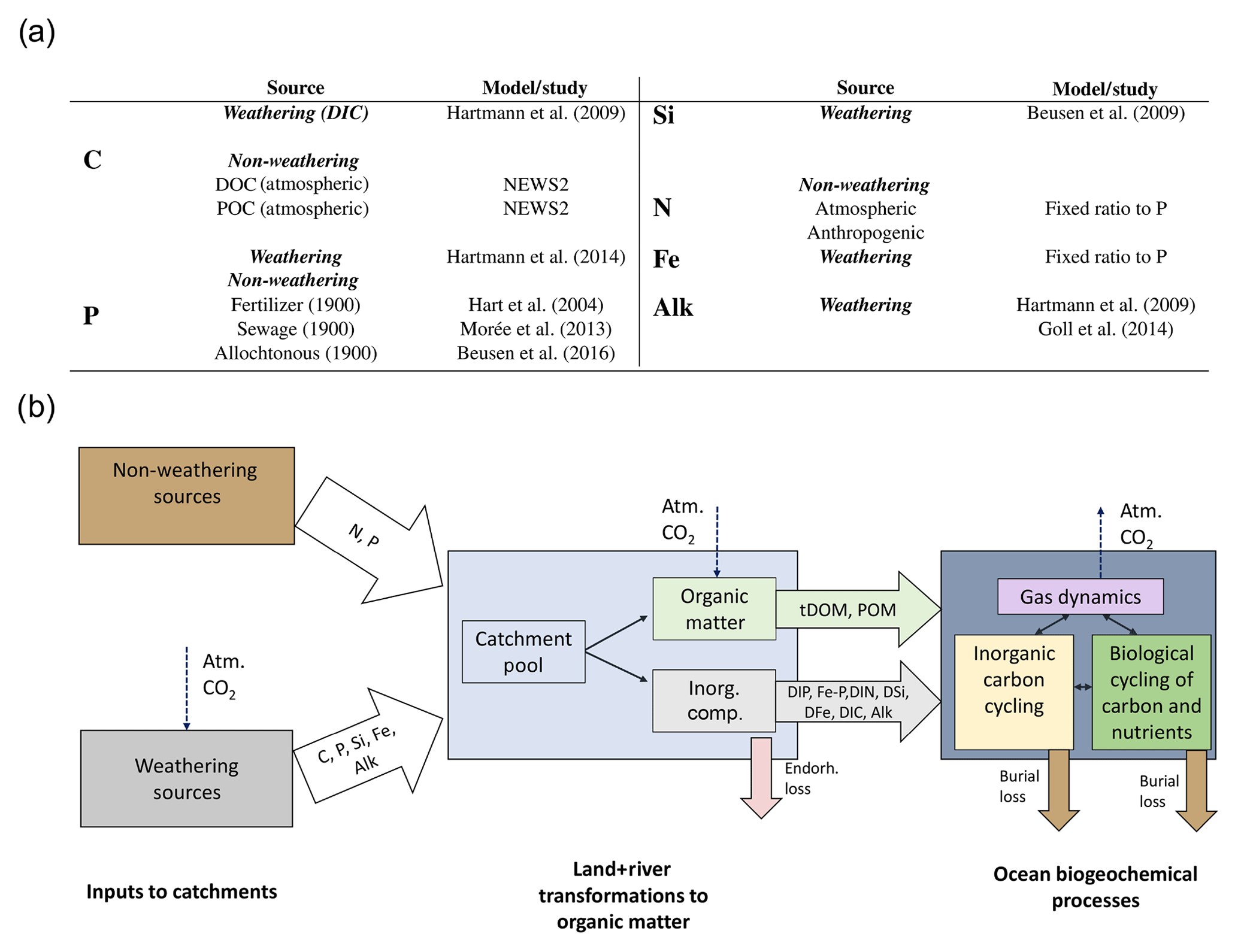
Figure 1(a) Table of sources of nutrient, carbon and alkalinity inputs to river catchments and (b) scheme of origins and transformations of the catchment compounds, as well as biogeochemical processes in the ocean in our framework. The abbreviations are: Inorg. Comp.: Inorganic Compounds, tDOM: terrestrial dissolved organic matter, POM: particulate organic matter, DIP: dissolved inorganic phosphorus, Fe-P: iron-bound phosphorus, DIN: dissolved inorganic nitrogen, DSi: dissolved silica, DFe: dissolved iron, DIC: dissolved inorganic carbon, Alk: alkalinity.
2.1.2 Phosphorus
P weathering yields
We derived the P weathering yields from a spatiotemporal model (Hartmann et al., 2014), which quantifies the P weathering release in relation to the SiO2 and cation release induced by weathering. The model was originally calibrated for the extensive data set of 381 river catchments of the Japanese Archipelago with runoff and lithological characteristics (Hartmann and Moosdorf, 2011) being used as sole model variables. The model was then corrected for temperature and soil shielding effects at the global scale (Hartmann et al., 2014):
where FPrelease is the chemical weathering rate of P per area (t km−2 yr−1), bP,i is an empirical factor representing the rate of P weathering of the lithology i, q is the surface runoff (mm yr−1), Fi(T) is a lithology-dependent temperature function and FS is a parameter to account for soil shielding.
The lithology types consisted of 16 lithological classes from the global lithological database GliM (Hartmann and Moosdorf, 2012). The lithology-dependent factor bP,i represents the chemical weathering rate factor for SiO2 + cations () multiplied with the relative P content (bPrel,i):
The parameters and bPrel,i for each lithology i can be found in Hartmann et al. (2014).
The temperature correction function F(T) is an Arrhenius relationship for basic (rich in iron and magnesium) and acid (high silica content) lithological classes, with activation energies normalized to the average temperature of the calibration catchments of the study (Hartmann et al., 2014). For acid rock lithologies, an activation energy of 60 kJ mol−1 was assumed, whereas for basic rock types 50 kJ mol−1 was used. Carbonate lithologies do not have a temperature correction function due to the absence of a clear relationship to field data, as well as due to uncertainties in the mechanisms of a temperature effect on carbonate weathering (Hartmann et al., 2014; Romero-Mujalli et al., 2018).
A soil shielding factor FS was considered to represent the inhibition of weathering by certain types of soils. These soils, which have low physical erosion rates, develop a chemically depleted thick layer, shielding them from water supply and thus partly preventing the weathering of the soil aggregates (Stallard, 1995). An average soil shielding factor of 0.1 was estimated for the soils Ferrasols, Acrisols, Nitisols, Lixisols, Histosols and Gleysols while performing a calibration at the global scale in Hartmann et al. (2014).
Non-weathering P sources
Since the P cycle was already perturbed in the assumed pre-industrial state (1850) due to anthropogenic activities (Mackenzie et al., 2002; Filippelli, 2008; Beusen et al., 2016), we also accounted for P sources other than weathering (Pnw,catch). Similarly to Beusen et al. (2016), we derived the non-weathering catchment source of P as the sum of fertilizer (Pfert,catch), sewage (Psew,catch) and allochthonous P inputs (Palloch,catch):
Pfert,catch was the P input to river catchments originating from the agricultural application of fertilizers, manure and organic matter (1.6 Tg P yr−1 globally, from Beusen et al., 2016); Psew,catch was the P input from sewage (0.1 Tg P yr−1 globally, Morée et al., 2013) and Palloch,catch represented allochthonous organic matter P inputs (1 Tg P yr−1, which were simplified as vegetation in floodplains in Beusen et al., 2016). All of these P inputs were estimated for year 1900 due to previous estimates not being available to our knowledge. Since our framework was developed with the aim of being used in ESMs, we assumed soil equilibrium since this is the initial state criteria used in state-of-the-art model simulations. Therefore, P exports due to perturbations of organic matter erosion in soils were not considered. The global distribution of anthropogenic P inputs (agricultural + sewage) to catchments was assumed to be the same as the distribution of contemporary anthropogenic P inputs, which were derived from the NEWS2 study:
where Pant,global is the global sum of anthropogenic P inputs to catchments, whereas DIPant-pd,catch and DIPant-pd,global are anthropogenic inputs from the NEWS2 study (1970) for every catchment and their global sum, respectively. Regarding the allochthonous P inputs, we assumed the same global distribution as for the organic matter yields. Both of these distributions are shown and discussed in the Supplement S1.1 and S1.2.
P river loads
For each catchment, we estimated the annual P exports of the individual catchments (Ptotal,catch) as the sum of the catchment weathering yields (Pw,catch) and of non-weathering catchment P inputs (Pnw,catch):
Ptotal,catch was then fractionated into inorganic P (IPcatch) and organic P bound within tDOM (DOP) and POM (POP), which were assumed to have been taken up on land or in freshwaters by the biology at the prescribed fixed organic C:P ratio. The remaining catchment P was assumed to be IPcatch:
The IP was thereafter fractionated into DIP and Fe-P (IP bound to iron-manganese oxide and hydroxide) at a ratio rinorg (DIP : Fe-P = 1:3, approximated from the pre-industrial global export estimates of Compton et al., 2000) and (1−rinorg):
and
We did not consider detrital particulate inorganic P exports from the physical weathering of rock. This P is not bioavailable in rivers or in the coastal ocean due to strong covalent bonds of the detrital mineral structures (Compton et al., 2000).
2.1.3 Nitrogen and iron
The N inputs to river catchments were derived from a globally fixed mole N:P ratio of 16:1 (Takahashi et al., 1985) with regard to P inputs for all species (DIN:IP, N:P in tDOM and N:P in POM). In published literature, higher N:P ratios for all riverine species exports are suggested, with Beusen et al. (2016) simulating a pre-industrial N:P mole ratio of 21:1 and Turner et al. (2003) reporting higher N:P ratios of over 16:1 in a synthesis of measurements in major rivers. However, denitrification in river estuaries, which is not taken into account in the mentioned studies, also removes N (3–10 Tg N yr−1, Seitzinger et al., 2005). According to our calculations, this estuarine N sink could reduce the N:P ratio of the global exports to around 16:1 (Supplement S1.3). For Fe, we used a P:Fe mole ratio of , which is the Fe:P export ratio of organic matter in the ocean biogeochemistry model, to quantify Fe inputs to catchments for all species (IP:DFe, P:Fe in tDOM and P:Fe in POM). The iron of the Fe-P iron-manganese oxides and hydroxides was not considered to be bioavailable.
2.1.4 Dissolved inorganic carbon and alkalinity
The DIC and Alk weathering release, as well as the drawdown of atmospheric CO2 induced by weathering, were quantified according to the studies of Hartmann et al. (2009) and Goll et al. (2014). Weathering reactions cause an uptake of atmospheric CO2 and a release of DIC as during carbonate weathering
and silicate weathering
The Eqs. (9) and (10) dictate the release of 1 mol (thus 1 mol DIC and 1 mol Alk) for each mole of CO2 taken up during the weathering of silicate lithologies, and of 2 mol (thus 2 mol DIC and 2 mol Alk) for the uptake of each mole of CO2 drawn down during the weathering of carbonate lithologies.
The release equations from Hartmann et al. (2009) and Goll et al. (2014) quantify the lithology (i) dependent weathering release as a function of surface runoff (q), temperature (Fi(T)), soil shielding FS and a weathering parameter bC,i:
The parameter bC,i is dependent on the weathering rate of the lithology and the composition of the lithology.
The catchment DIC and Alk catchment loads were the weathered annually within the catchments, assuming conservation of Alk along the land–ocean continuum (Amiotte Suchet and Probst, 1995). We therefore assumed a DIC:Alk loads ratio of 1:1, without considering additional DIC sources from respiration of organic matter in soil pore water, groundwater or in rivers. River observational data however show that the riverine and total DIC mole exports rarely deviate by more than 10 % (Meybeck and Vörösmarty, 1999; Araujo et al., 2014).
2.1.5 Silica
To quantify the global spatial distribution of riverine DSi exports, we used the model developed by Beusen et al. (2009):
where is the export of DSi (Tg SiO2 yr−1 km−2), ln(prec) is the natural logarithm of the precipitation (mm d−1), volc is the area fraction covered by volcanic lithology (no dimension), bulk is the bulk density of the soil (Mg m−3), slope is the average slope (m km−1), and bprec, bvolc, bbulk and bslope are the regression coefficients estimated in Beusen et al. (2009). For the precipitation, we used the pre-industrial model output from the MPI-ESM, whereas the volcanic area originated from Dürr et al. (2005), the soil density from Batjes (1997) and Batjes (2002), and the average slope from the Global Agro-Ecological Zones database (FAO/IIASA, 2000). The exports were aggregated for the HD model catchment areas. The loads that were generated by applying the Beusen et al. (2009) model were also converted to teragrams silicon (Tg Si) and are given accordingly in our study. We approximated the weathering release of Si using this DSi model output, therefore assuming that sinks of Si on land or in rivers are compensated by sources from these ecosystems (a further equilibrium assumption). We also neglected the riverine exports of particulate Si originating from physical erosion.
2.2 Ocean model setup
2.2.1 Ocean biogeochemistry
The Max Planck Institute Ocean Model (MPIOM, Jungclaus et al., 2013), which was used to simulate oceanic physics, is a z coordinate global circulation model. It solves primitive equations under the hydrostatic and Boussinesq approximation on a C-grid with a free surface for every model time step (1 h). The grid configuration used in this study (GR15) consists of a bipolar grid with one pole over the Antarctic and one over Greenland. It resolves the ocean horizontally at around 1.5∘ and through 40 unevenly spaced vertical layers with increasing thicknesses at greater depths. The flow fields of the MPIOM dictate the advection, mixing and diffusion of biogeochemical compounds in the ocean. The atmospheric surface boundary data, as well as river freshwater model inputs, which are used to drive MPIOM here, originate from the Ocean Model Intercomparison Project (OMIP, Röske, 2006). The atmospheric forcing data set is a mean annual cycle for atmospheric parameters at a daily time step constructed from ECMWF reanalysis project ERA-40 data. For the freshwater forcing climatology, the HD model was driven with the ERA-40 atmospheric data (Hagemann and Gates, 2001).
The Hamburg Ocean Carbon Cycle model (HAMOCC) simulates the inorganic carbon chemistry, biological transformations, nutrient cycling and gas dynamics in the oceanic water column, sediment and at the air–sea interface. The model core along with its equations are described in Ilyina et al. (2013), but we also accounted for more recent modifications explained in Mauritsen et al. (2018). These included incorporating dynamic nitrogen fixation by cyanobacteria (Paulsen et al., 2017), following recommendations of the OMIP protocol (Orr et al., 2017) and including nitrogen deposition according to the Coupled Model Intercomparison Project 6 (CMIP6) database (https://esgf-node.llnl.gov/projects/input4mips/, last access: 17 December 2019). The pools of the model consist of DIP, DIN, DFe, O2, DSi, DIC, Alk, opal, calcium carbonate (CaCO3), phytoplankton (PHY), cyanobacteria (CYA), dissolved organic material (DOM) and particulate organic material (POM) (Appendix A1).
The inorganic carbon chemistry is based on Maier-Reimer and Hasselmann (1987), with adjustments in the calculation of chemical constants as described in the OMIP protocol (Orr et al., 2017). Total DIC and total Alk are thereby prognostic tracers from which the carbonate species are determined diagnostically. Total DIC includes all carbonate species and total Alk includes carbonate as well as borate alkalinity.
The dynamics of organic matter cycling in the ocean are based on an NPZD (nutrients, phytoplankton, zooplankton, detritus/POM) model extended with pools for DOM and cyanobacteria. The phytoplankton growth follows Michaelis–Menten kinetics as a function of temperature, light and nutrient availability. A constant ratio (, Takahashi et al., 1985) dictates the composition of all oceanic organic matter. Both oceanic DOM and POM are advected according to the ocean physics, and the POM also sinks as a function of depth (Martin et al., 1987). The aerobic remineralization of organic matter takes place when the O2 concentration is above a threshold, whereas at low enough O2 concentrations, denitrification and sulfate reduction can take place. Furthermore, the phytoplankton produce opal shells when dissolved silica is available, and CaCO3 shells when dissolved silica is depleted. The CaCO3 and opal shells sink at constant rates.
HAMOCC also contains a 12-layer sediment module that simulates the same remineralization and dissolution processes as in the water column for sediment constituents (Heinze et al., 1999). The sediment consists of a fraction of pore water, which contains dissolved inorganic compounds (e.g., DIC and DIP). POM, CaCO3 and opal fluxes from the water column are deposited to the top sediment layer. There is a diffusive inorganic compound flux at the water-sediment interface and a particulate flux from the bottom layer to a diagenetically consolidated burial layer.
Dust is added through atmospheric deposition according to input fields of Mahowald et al. (2006). The model considers the dynamics of CO2, O2, N2O and N2 and their exchange at the ocean–atmosphere interface. Since we modeled a pre-industrial state in this study, we used constant atmospheric concentrations for CO2 of 278 ppmv (Etheridge et al., 1996).
2.2.2 Treatment of the river loads in the ocean biogeochemistry model
The biogeochemical riverine loads were added to the ocean surface layer in HAMOCC constantly over the whole year. The locations of major river mouths were manually corrected on a case-to-case basis for large rivers in order to reproduce the same locations as of the OMIP freshwater inputs.
The riverine dissolved inorganic compounds (DIC, Alk, DIP, DIN, DSi, DIC, DFe) were added to the HAMOCC in their species pools. We added 80 % of P contained in the riverine Fe-P to the oceanic DIP pool in order for the amount of bio-available Fe-P to be comparable to the estimated range given in Compton et al. (2000) (1.1–1.5 Tg P yr−1). The rest of the Fe-P pool was considered to be unreactive in the ocean. The riverine POM was added to the oceanic POM pool in HAMOCC.
For tDOM, we extended HAMOCC with a new model tracer that was characterized by the described mole ratio. tDOM was mineralized as a function of the tDOM concentration at a rate constant krem,tDOM and of an oxygen limitation factor (), which decreases the maximum potential remineralization rate depending on the O2 concentration:
Since a large fraction of tDOM delivered by rivers is already strongly degraded, it is to a certain extent resistant to microbial degradation in the ocean (Ittekkot, 1988; Vodacek et al., 2003). We therefore assumed a slightly lower remineralization rate constant of tDOM (krem,tDOM) compared to oceanic DOM (0.003 versus 0.008 d−1 for oceanic DOM). This rate constant is within the range provided for the Louisiana shelf in Fichot and Benner (2014) (0.001–0.02 d−1), and we also compared open ocean tDOM concentrations to the limitedly available observational data in Supplement S2.2. The O2 limitation function used (ΓO2) was the same as the function used for oceanic DOM, which is described in Mauritsen et al. (2018).
2.2.3 Pre-industrial ocean biogeochemistry model simulations
We performed two ocean model simulations in order to assess the impacts of biogeochemical riverine fluxes in terms of their magnitudes and locations: REF and RIV.
REF was performed using the standard model version until now (for instance in Mauritsen et al., 2018), which was lacking in terms of its representation of riverine inputs: Biogeochemical inputs were added to the entire surface ocean in order to compensate for sediment burial losses at the global scale. This was done with the reasoning that in HAMOCC, biogeochemical inputs are needed in order to maintain a stable ocean state, since the burial loss in the sediment induces a loss of CaCO3, opal and POM. Without these model inputs, ocean biogeochemical pool inventories would thrive to zero. In order to maintain a state close to equilibrium in the standard model version (REF), inputs representing the redissolution of CaCO3 (added in a mole Alk:DIC ratio of 2:1), inputs of DSi and inputs of oceanic DOM were therefore added homogeneously per area to the entire surface ocean in the magnitudes of the global sediment losses. Therefore, the inputs were almost solely added to the open surface ocean, since it covers 94 % of the total ocean area in the model (see Supplement S5). REF was performed for 5000 years, where burial fluxes were computed approximately every 1000 years. The fluxes resulting from these calculations were added to the ocean at every model time step.
The simulation RIV replaced the homogeneous inputs of Alk:DIC, DSi and oceanic DOM to the ocean surface computed from burial losses with riverine inputs of DIP, Fe-P, DIN, DSi, DFe, DIC, Alk, tDOM and POM, which were derived in the described approach. The major differences to the REF simulation originate from the geographic locations of the inputs, the magnitudes of C loads to the ocean, as well as from the riverine mole ratios of Alk:DIC in comparison to the CaCO3 burial compensation inputs (1:1 for RIV and 2:1 for REF) and of tDOM () in comparison to the oceanic DOM inputs (). Since the riverine inputs to the ocean were fully constrained by our calculations in RIV, long simulations were needed to equilibrate both the water column and the sediment to the new biogeochemical inputs. We performed a simulation for 4000 years first, including both the water column and sediment model components. Once particulate fluxes to the sediment were approximately stable, we used the 100-year mean of these fluxes to perform a 10 000-year simulation of the sediment sub-model. The resulting sediment state was then coupled back to the water column for a simulation of 2000 more years.
We used REF as a reference simulation in order to compare RIV to, which enabled us to compare the impacts of riverine loads at plausible pre-industrial magnitudes and locations (RIV) to REF, where the vast majority of inputs were added directly to the open ocean. For the analysis of the resulting ocean biogeochemistry, we used the last 100-year means of RIV and REF.
2.3 Definitions of coastal regions for analysis
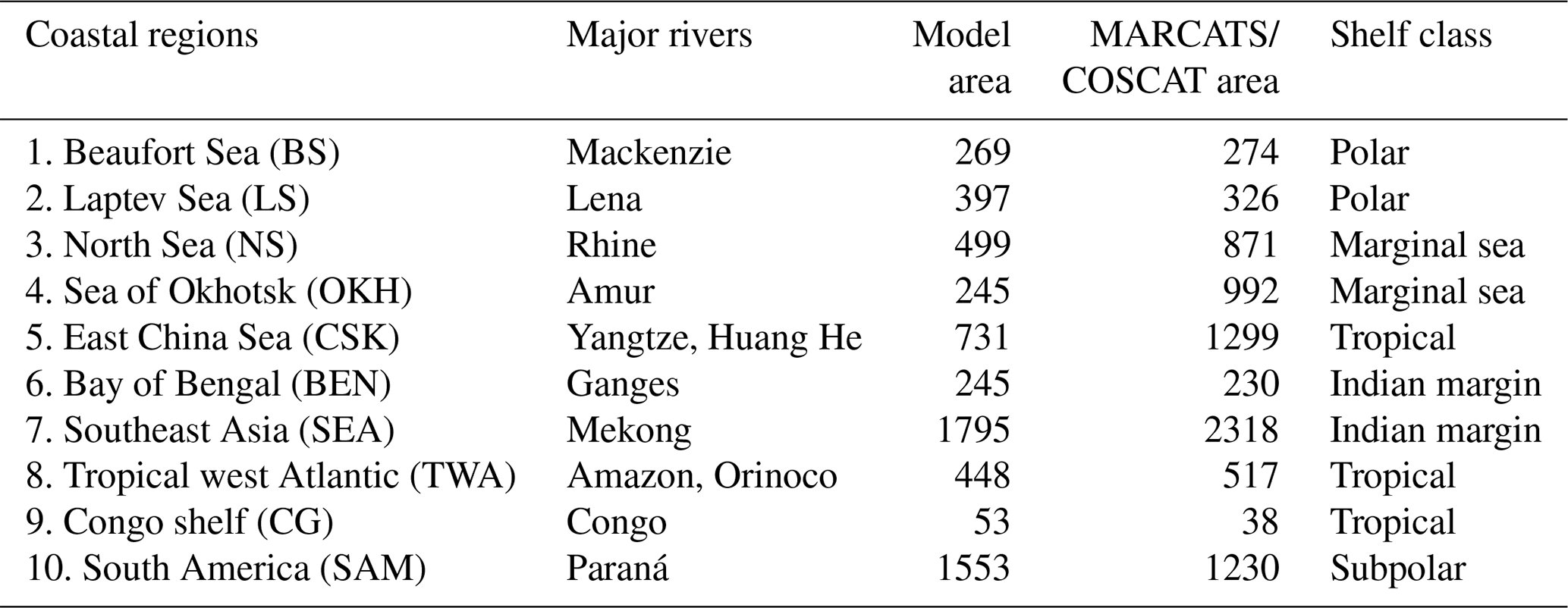
To investigate the impacts of riverine exports on coastal regions, we selected 10 shallow shelf regions characterized by large riverine loads that cover a variety of latitudes (Table 1). The shelves were defined to have depths of less than 250 m. The cutoff sections perpendicular to the coast were done according to MARgins and CATchments Segmentation (MARCATS) (Laruelle et al., 2013), except for the Beaufort Sea, Laptev Sea, North Sea and Congo shelf, where we used the COastal Segmentation and related CATchments (COSCATs) definitions (Meybeck et al., 2006) due to the vastness of their MARCATS segmentations.
Table 1Comparison of the surface areas (109 m2) of selected coastal regions with depths of under 250 m in the ocean model setup and in the segmentation approaches. The comparisons were done with the MARCATS (Laruelle et al., 2013) or COSCATs (Beaufort Sea, Laptev Sea, North Sea, Congo shelf, Meybeck et al., 2006). The shelf classes were defined as in Laruelle et al. (2013).
3.1 Global weathering release
The weathering release models provide global annual means for the pre-industrial weathering release of P, Si, DIC and Alk (Table 2), as well as their spatial distributions (Fig. 2). The calculated global P release is 1.34 Tg P yr−1 when considering the runoff scaling factor of 1.59, which fits within the P release range of 0.8–4 Tg P yr−1 reported in published literature (Compton et al., 2000; Wang et al., 2010; Goll et al., 2014; Hartmann et al., 2014). While the Hartmann et al. (2014) and Goll et al. (2014) estimates (1.1 and 0.8–1.2 Tg P yr−1, respectively) originate from the same weathering model as is used here, the 1.9 Tg P yr−1 value reported in Wang et al. (2010) was constructed by upscaling measurement data points. In a further study, Compton et al. (2000) provide a quantification of the prehuman phosphorus cycle while distinguishing between land–ocean fluxes from shale-erosion as well as from weathering. The reported total prehuman riverine P export with a weathering source is given by averaging non-detrital P species concentrations from unpolluted rivers and multiplying them with global runoff estimates, thereby yielding an estimate of 2.5–4.0 Tg P yr−1. Both estimates that originate from the upscaling of river measurements are therefore higher than the P weathering fluxes provided in the modeling approach in this study, in Goll et al. (2014) and in Hartmann et al. (2014), which suggests further effort might be needed to constrain the global P weathering release more accurately.
For Si, we model a global release of 168 Tg Si yr−1. This is within the range estimated by Beusen et al. (2009) (158–199 Tg Si yr−1), who used the same model while using present-day observational data to drive the model for precipitation. Our estimate is also comparable to the 173 Tg Si yr−1 value reported by Dürr et al. (2011).
The modeled DIC and Alk release amount to 374 Tg C yr−1 and 37.8 Teq yr−1 globally, which also take into account the runoff scaling factor. By extrapolating from measurement data of 60 large river catchments, Meybeck (1982) suggests that the global DIC export to the ocean is around 380 Tg yr−1 and originates directly from weathering. Further modeling studies also provide similar weathering release estimates of 260 to 300 Tg C yr−1 (Berner et al., 1983; Amiotte Suchet and Probst, 1995). The atmospheric CO2 drawdown induced by weathering is directly related to the weathering release of DIC, since silicate weathering draws down 1 mole of CO2 per mole , and carbonate weathering draws down 0.5 mol of CO2 per mole released (Eqs. 9 and 10). While we model a CO2 drawdown flux of 280 Tg C yr−1 induced by weathering, drawdown fluxes of 220–440 Tg C yr−1 are reported in published literature (Gaillardet et al., 1999; Amiotte Suchet et al., 2003; Hartmann et al., 2009; Goll et al., 2014). The results imply that, of the 374 Tg C yr−1 DIC released by weathering, 280 Tg C yr−1 originates from atmospheric C drawdown, while the rest originates from the weathering DIC release from the carbonate lithology (94 Tg C yr−1).
Table 2Global pre-industrial weathering release of P, Si, DIC and Alk, as well as CO2 drawdown, modeled in this study and previously estimated in published literature.
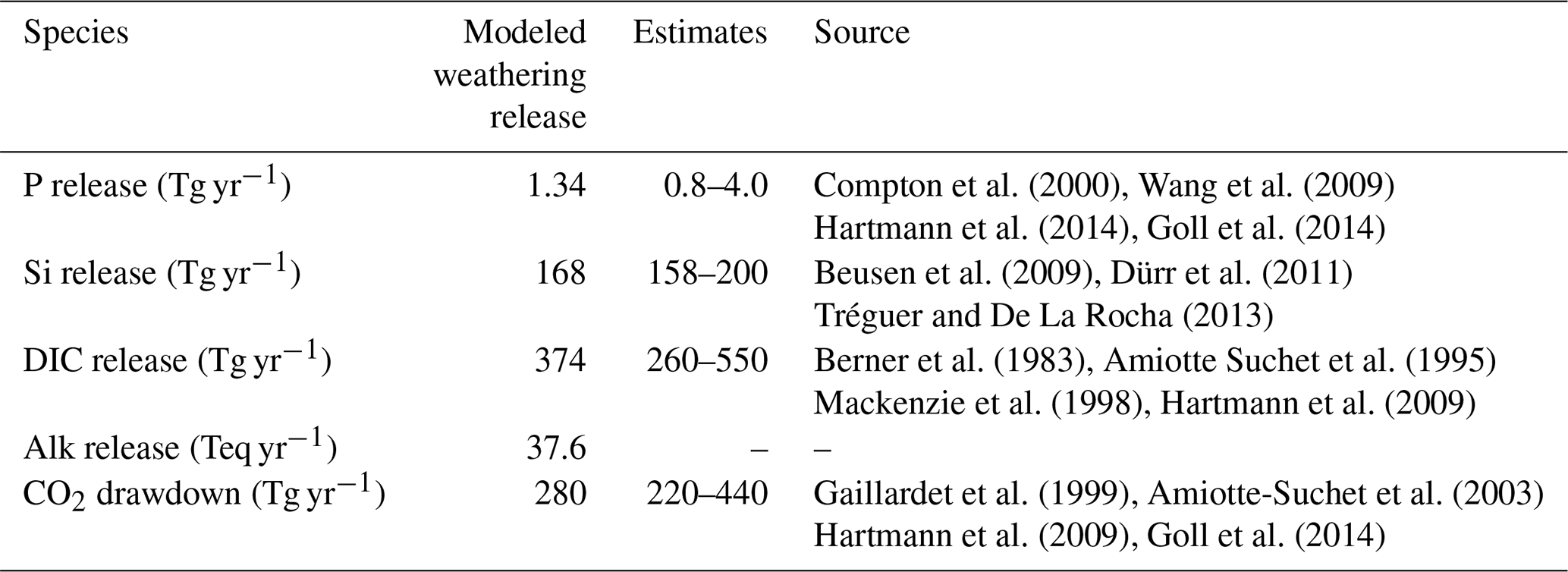
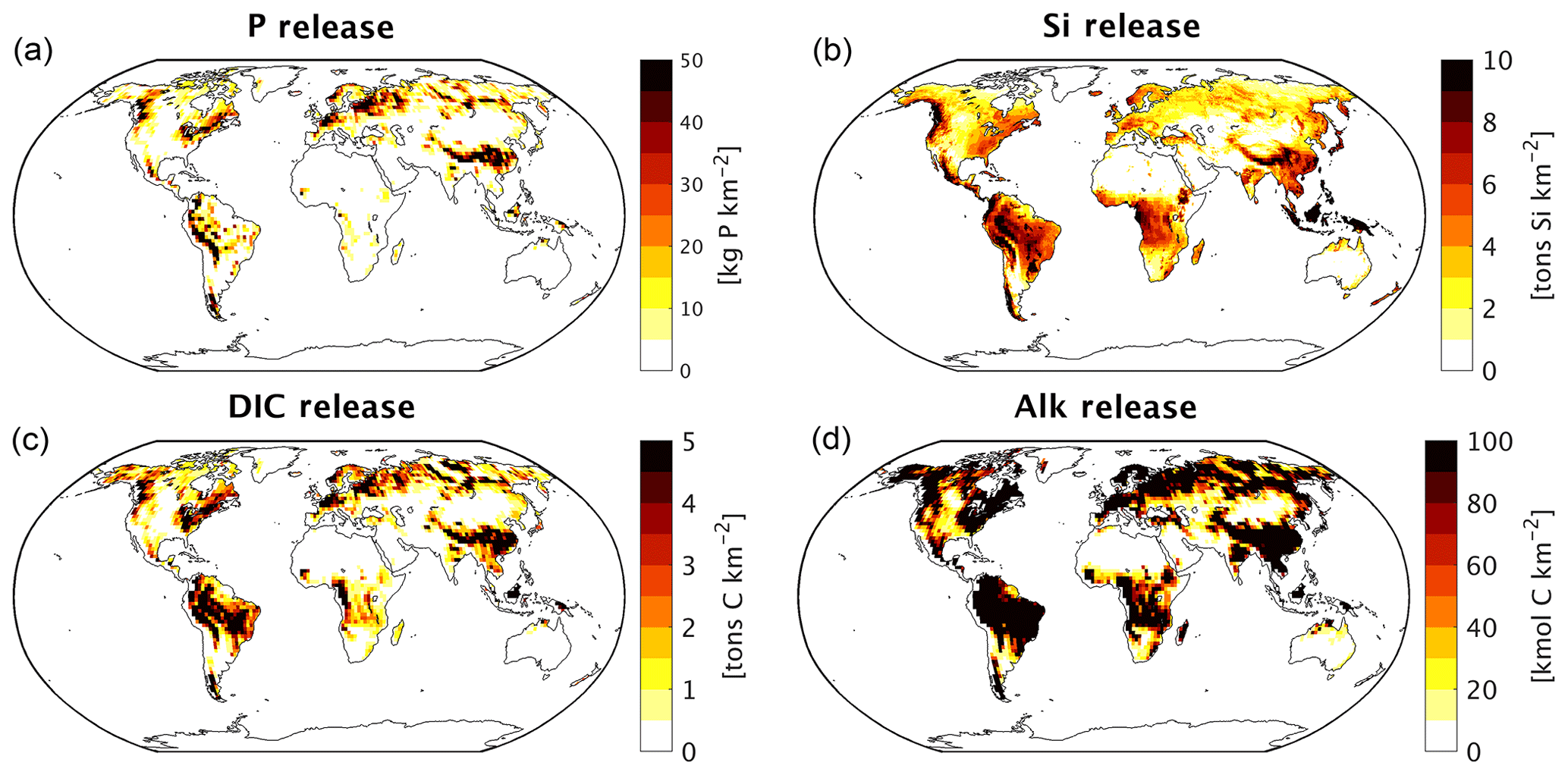
Figure 2Weathering release yields of (a) P (kg P km−2), (b) Si (t Si km−2) and (c) DIC (t C km−2).
We observe hotspots that contribute disproportionately to the weathering release yields, with the Amazon, Southeast Asia as well as northern Europe and Siberia acting as strong sources of weathering (Fig. 2). The disproportionate importance of these regions for the global weathering release is largely due to wet and/or warm climates, as well as to their lithological characteristics (Amiotte Suchet and Probst, 1995; Gaillardet et al., 1999; Hartmann and Moosdorf, 2011).
3.2 Global riverine loads in the context of published estimates
In our modeling framework, the global pre-industrial riverine exports to the ocean amount to 3.7 Tg P yr−1, 27 Tg N yr−1, 158 Tg Si yr−1 and 603 Tg C yr−1, whereas 0.3 Tg P, 2.2 Tg N, 10 Tg Si and 19 Tg C are retained in endorheic catchments. The fraction of Fe-P assumed to not desorb in the coastal ocean was also subtracted from the global loads (0.2 Pg P yr−1).
Table 3Comparison of modeled global riverine loads (Model. global loads) with previous estimates (Tg yr−1). The total loads thereby exclude particulate inorganic loads, except for the 1970 POP estimate, which includes all particulate P compounds from the NEWS2 study. Fe-P only considers all particulate P (PP) that is assumed to be desorbed in the ocean. The PP value from the NEWS2 study considers both POP as well as particulate inorganic phosphorus.
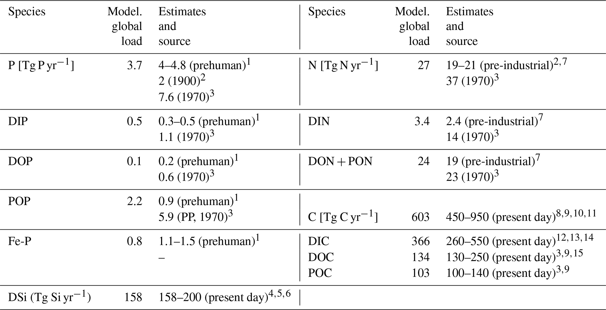
1 Compton et al. (2000). 2 Beusen et al. (2016). 3 NEWS2 (Seitzinger et al., 2010). 4 Beusen et al. (2009). 5 Dürr et al. (2011). 6 Tréguer and De La Rocha (2013). 7 Green et al. (2004). 8 Jacobson et al. (2007). 9 Meybeck and Vörösmarty (1999). 10 Resplandy et al. (2018). 11 Regnier et al. (2013). 12 Berner et al. (1983). 13 Amiotte Suchet and Probst (1995). 14 Mackenzie et al. (1998). 15 Cai (2011).
In the following, we compare the magnitudes of the modeled pre-industrial riverine exports of P, N, Si and C, as well as of their fractionations, with a wide range of estimates found in published literature (Table 3). This was done in comparison to pre-industrial estimates directly, as well as to 1970 estimates by the NEWS2 study, in order to assess the modeled loads in the context of present-day estimations.
The modeled global P loads are slightly below the P export estimate range of 4–4.7 Tg P yr−1 reported in Compton et al. (2000), which was constructed by scaling measured catchment P loads of pristine rivers to the global river freshwater discharge (thus prehuman). A recent modeling study by Beusen et al. (2016), which takes P retention processes in rivers into account, suggests a lower global load of 2 Tg P yr−1 for the year 1900. The 1970 estimate (7.6 Tg P yr−1) provided by the NEWS2 study, which considers substantial anthropogenic P inputs, nevertheless suggests a steep 20th century increase in the global P export to the ocean when considering all three pre-industrial estimates. The modeled DIP export to the ocean (0.5 Tg P yr−1) is situated at the top range of the prehuman estimates (0.3–0.5 Tg yr−1) and well below estimates for the year 1970 (1.1 Tg P yr−1). A direct fractionation of the global P flux to DIP, DOP and POP is not provided in the Beusen et al. (2016) study. Furthermore, we estimate similar global loads of DOP to Compton et al. (2000) (around 0.1 and 0.2 Tg P yr−1, respectively). The modeled DOP value is also much lower than the 1970 DOP estimate (0.6 Tg P yr−1), which is realistic due to the human-caused increase of DOP loads during the 20th century (Seitzinger et al., 2010). The modeled POP global load is larger than the estimate of Compton et al. (2000), which could be due to the POM C:P ratio of 122:1 chosen in our study. Strong uncertainties exist in the global C:P ratios for riverine POM, with Meybeck (1993) suggesting a mole ratio of around 56 C:P, whereas Ramirez and Rose (1992) estimate a ratio of around 499, which would strongly affect the results given here. The particulate P load given in the NEWS2 study is vastly higher than the POP load modeled in our study, but a large fraction of the estimate is likely detrital particulate P, which we do not account for in the present study. The modeled Fe-P (1.0 Tg P yr−1) is slightly below the range estimated in Compton et al. (2000) (1.5–3.0 Tg P yr−1). However, the assumed reactive fraction of the Fe-P loads (0.8 Tg P yr−1) here is close to how much Fe-P is suggested to be desorbed in the coastal ocean in Compton et al. (2000) (1.1–1.5 Tg P yr−1).
Despite our simplified assumption of N loads being directly coupled to P loads, the modeled global N load is situated within the prehuman and contemporary land–ocean N load estimates modeled in Green et al. (2004) (21 and 40 Tg N yr−1, respectively). The modeled annual DIN load (3.4 Tg N) is slightly higher than the prehuman load given in the Green et al. (2004) study (2.4 Tg N yr−1). In Beusen et al. (2016), the global pre-industrial N load is suggested to be lower (19 Tg N yr−1) due to in-stream retention and removal of N.
Since we assume that the change in the global DSi load over the 20th century is small, we directly compare our modeled pre-industrial DSi load estimate with present-day DSi load estimates from published literature. The modeled global load of DSi is 158 Tg Si yr−1 in our framework, which is situated at the low end of the present-day estimate range of 158–200 Tg Si yr−1. The NEWS2 study used the same Beusen et al. (2009) DSi export model forced with present-day observational precipitation data. Dürr et al. (2011) and Tréguer and De La Rocha (2013) upscaled from discharge-weighted DSi concentrations at river mouths. Substantial amounts of particulate Si are suggested to be delivered to the ocean, yet it is not clear how much of it is dissolvable in the ocean (Tréguer and De La Rocha, 2013), and, therefore, particulate Si is not considered in our study. The effects from contemporary increases in river damming on global DSi loads are also uncertain. Increased damming could have increased the global silica retention in rivers (Ittekkot et al., 2000; Maavara et al., 2014). Therefore, the global pre-industrial DSi load to the ocean could potentially have been larger than for the present day, but quantifying the implications of damming for the in-stream retention of DSi, as well as of suggested increased DSi inputs from weathering and from the terrestrial biosphere (e.g., Gislason et al., 2009) escape the scope of this study.
In our study, we also assumed that the pre-industrial C loads of all species were the same as for the present day. While the C retention along the land–ocean continuum might have increased during the 20th century, enhanced soil erosion through changes in land use might have also increased the C inputs to the freshwater systems, leaving question marks on the magnitude of the net anthropogenic perturbation (Regnier et al., 2013; Maavara et al., 2017). The modeled total C, DIC, DOC and POC fluxes agree with the present-day estimate ranges shown in Table 3 but are also situated at the lower end of these ranges. The organic C loads, which originate directly from the NEWS2 study, are particularly low.
The large spreads of the riverine export estimates underline difficulties in constraining pre-industrial riverine fluxes. Even for the present day, Beusen et al. (2016) note large differences between the simulated loads of their study and the previous global modeling study NEWS2. In turn, upscaling from point measurements are often based on data collected by Meybeck (1982) for the pre-1980 time period without taking into account more recent river measurement data. They also rely on the assumption of a linear relationship between riverine discharge and compound loads. While we acknowledge a certain degree of uncertainty in the numbers provided in this study, the modeling approach chosen nevertheless leads to global pre-industrial riverine loads that are in line with what was suggested previously and constitutes a framework that could be incorporated within state-of-the-art Earth system models.
3.3 Hotspots of riverine loads
We observe several regions of disproportionate contributions to global riverine loads (Fig. 3, Table 4), with a distribution largely following spatial patterns of the weathering release. Our framework reveals large differences between the riverine exports from the Northern Hemisphere and from the Southern Hemisphere. The Northern Hemisphere thereby accounts for an annual riverine C input of 404 Tg C to the ocean, vastly dominating the global loads (67 % of global riverine C), while the Southern Hemisphere delivers 199 Tg C (33 % global riverine C).
Rivers that drain into the tropical Atlantic basin consist of a major fraction of the global oceanic biogeochemical supply (Table 4). This is due to major rivers of the South American continent debouching into the ocean basin, as well as considerable exports provided by West African rivers. According to our framework, the annual C loads of the seven largest rivers debouching in the basin (Orinoco, Amazon, São Francisco, Paraíba do Sul, Volta, Niger and Congo) amount to 123 Tg C (fractionated into 58 Tg DIC, 44 Tg DOC, 21 Tg POC), which consists of around 20 % with respect to global riverine C exports. These regional C loads agree very well with estimated values derived from monthly data of Araujo et al. (2014) (53 Tg DIC, 46 Tg DOC). Of these major rivers, the pre-industrial Amazon river provides the largest input of biogeochemical tracers to the ocean (modeled annual loads of 0.07 Tg DIP, 0.5 Tg DIN, 15.2 Tg DSi, 33.2 Tg DIC, 28.3 Tg DOC Tg, 17.1 Tg POC), which compare well with the present-day data (0.22 Tg DIP, 17.8 Tg DSi, 32.7 Tg DIC, 29.1 Tg DOC, Araujo et al., 2014). For the other catchments debouching in the tropical Atlantic, the modeled DIC loads are close to estimated values for the Congo, Orinoco and Niger, but are overestimated for the smaller catchments of the Paraíba, Volta and São Francisco. Calculating the regional sum of the modeled pre-industrial and estimated present-day DIP loads reveals a much lower pre-industrial load (81.8×10⁹ g P yr−1) with respect to the total present-day load (276×109 g P yr−1), suggesting a realistic increase of 194×109 g P yr−1 due to anthropogenic perturbations.
Although less substantial in the context of global loads, major Arctic rivers (Yukon, Mackenzie, Ob, Lena, Yenisei) provide a large C supply to the Arctic Ocean, with a dominant fraction of the C load consisting of DIC. In our framework, these rivers provide 37.5 Tg DIC (10 % of global DIC), 14.4 Tg DOC (11 % of global DOC) and 4.4 Tg POC annually to the Arctic Ocean. The total riverine C loads to the Arctic therefore amount to 56 Tg C yr−1, thus 9 % of global C loads. The DIC, DOC and POC load levels are comparable to estimates of 29 Tg DIC yr−1 (Tank et al., 2012), 17 Tg DOC yr−1 (Raymond et al., 2007) and 5 Tg POC (Dittmar and Kattner, 2003). Total Arctic DIP loads (40.8×10⁹ g P yr−1) derived from our modeling approach are slightly higher with regard to the published literature estimate of 35.8×10⁹ g P yr−1. DIP inputs from anthropogenic sources are considered to be small for Arctic catchments (Seitzinger et al., 2010), which explains why the modeled pre-industrial DIP loads are of similar magnitudes to observed DIP loads for the present day. Modeled Arctic DIC and DIP loads, which are strongly affected by inputs from the weathering models used in this study, are slightly larger with respect to published literature estimates, suggesting that the runoff scaling factor of 1.59 that we applied within the weathering models might be too high for this region. Certain factors, such as the effects of permafrost on weathering rates, which could impact the dynamics of weathering in the region, also remain enigmatic (Hartmann et al., 2014).
Southeast Asian rivers also provide large loads of biogeochemical tracers to the ocean. The Huang He, Brahmaputra–Ganges, Yangtze, Mekong, Irrawaddy and Salween rivers, which have catchment areas characterized by warm and humid climates, provide 92.4 Tg C yr−1 to the ocean (15 % of global C loads). We observe vastly elevated DIP levels for the present-day estimates (76.4×10⁹ g P yr−1) with regards to our modeled pre-industrial loads (299×109 g P yr−1). The NEWS2 study suggests a strong present-day perturbation of the DIP loads due to anthropogenic inputs to the region's catchments (Seitzinger et al., 2010), which can plausibly explain these differences.
The Indo-Pacific islands have been identified as a region with much higher weathering yields than the global average (Hartmann et al., 2014). Although this region only accounts for around 2 % of the global land surface, it provides 7 % (39 Tg) of C and most notably 10 % of the global POC (10 Tg C) delivered by rivers to the ocean annually, making the region a stronger terrestrial source of POC than all Arctic catchments. Thus, the POM mobilization through soil erosion is likely a major driver of land–sea carbon exports in the region.
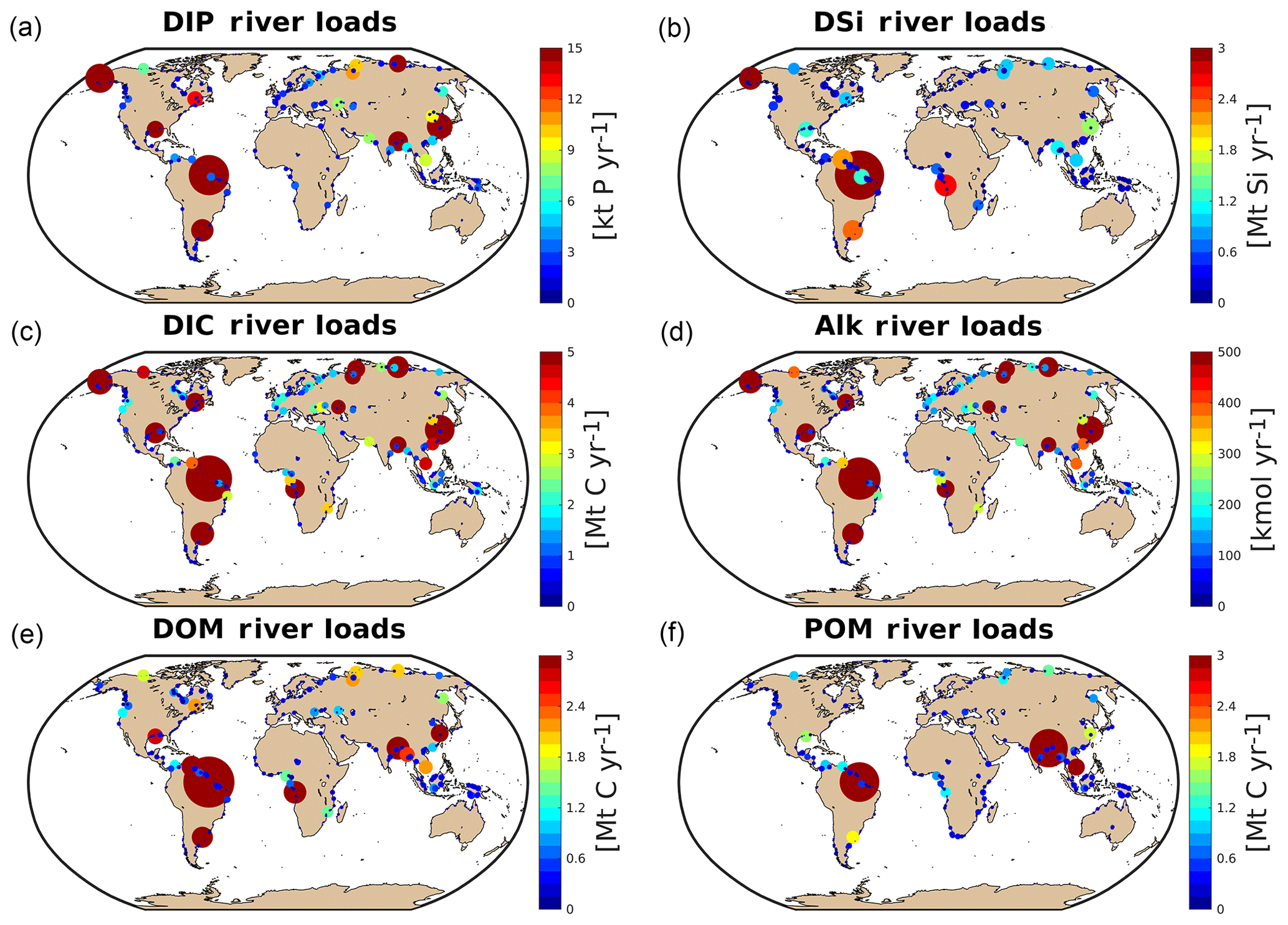
Figure 3Modeled annual river loads of DIP (a), DSi (b), DIC (c), Alk (d), DOM (e) and POM (f).
Table 4Regional hotspots of riverine C loads (Tg C yr−1) and DIP loads (109 g P yr−1) compared with regional estimates. Modeled DIP from our approach represents pre-industrial fluxes, whereas the DIP literature estimates are from present-day data and are strongly affected by anthropogenic perturbations.
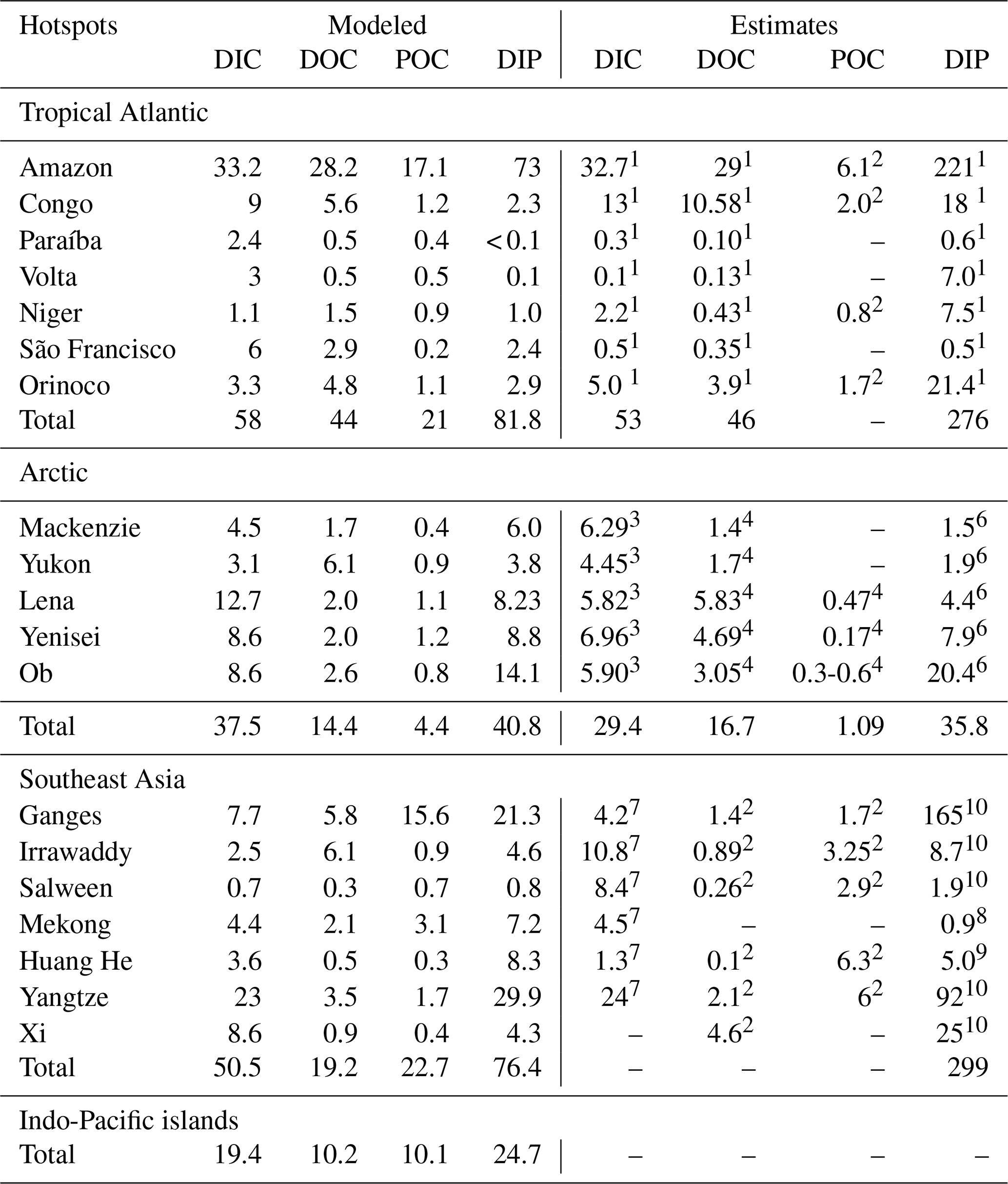
1 Araujo et al. (2014). 2 Bird et al. (2008). 3 Tank et al. (2012). 4 Raymond et al. (2007). 5 Dittmar and Kattner (2003). 6 Le Fouest et al. (2013). 7 Li and Bush (2015). 8 Yoshimura et al. (2009). 9 Tao et al. (2010). 10 Seitzinger et al. (2010).
4.1 The ocean state – an increased biogeochemical coastal sink
In the ocean simulations, the magnitudes of oceanic nutrient inputs (P, N and Si) do not strongly differ between REF and RIV (Table 5). This implies that in REF, the amounts of P, N and Si added to maintain a plausible ocean biogeochemical state were similar to what is derived in our approach to estimate pre-industrial riverine exports. Despite slightly larger P and N inputs in RIV than in REF, RIV simulates lower global surface dissolved P and N concentrations, and lower global NPP. The coastal ocean therefore must act as an increased biogeochemical sink in RIV, since the produced organic matter reaches the shallow coastal sea floor faster than in the open ocean, which allows for less time for the organic matter to be remineralized within the water column. This is confirmed by the increased organic matter flux to the global coastal sediment (defined as areas with less than 250 m depths), with an increase from 0.18 Gt C yr−1 (REF) to 0.25 Gt C yr−1 (RIV). The global coastal POM deposition range given in a review by Krumins et al. (2013) shows a large degree of uncertainty (0.19–2.20 Gt C yr−1), but nevertheless hints that the coastal POM deposition flux is possibly improved in RIV.
While Alk inputs were also added at nearly the same levels in REF as in the calculated riverine loads of RIV, the global C inputs are on the other hand increased by almost 100 % in RIV in comparison to REF. The inorganic (366 Tg C yr−1) and organic (237 Tg C yr−1) C inputs in RIV show stronger agreement with the riverine inorganic (260–550 Tg C yr−1) and organic C (270–350 Tg C yr−1) global load estimates found in literature (Meybeck, 1982; Amiotte Suchet and Probst, 1995; Mackenzie et al., 1998; Meybeck and Vörösmarty, 1999; Hartmann et al., 2009; Seitzinger et al., 2010; Cai, 2011; Regnier et al., 2013), signifying an improvement in the model's C inputs with respect to REF. These higher C inputs also result in a net long-term outgassing flux (231 Tg C yr−1), which is suggested in literature for the pre-industrial time period and is absent in REF. The net outgassing largely originates from higher DIC:Alk ratios of the riverine inputs (1:1) than is exported through the net CaCO3 production (1:2), as well as higher C:P ratios of tDOM inputs (2583:1) than is exported in the oceanic organic ratio (122:1). Both of these imbalances between oceanic input and export ratios lead to an increase of the pCO2 and CO2 outgassing in the long term (see Appendix C2).
Table 5Comparison of global oceanic inputs and global ocean biogeochemical state variables for REF and RIV. Additionally, we compare the modeled global mean surface DIP, DIN and DSi concentrations with World Ocean Atlas 2013 (WOA) surface layer means. OMZs: oxygen minimum zones.

The simulated global mean surface DIP and DIN concentrations are lower in RIV than in the observational data of the World Ocean Atlas 2013 (WOA) (0.439 and 0.480 µM DIP and 3.90 and 5.04 µM DIN respectively; WOA, Boyer et al., 2013), whereas the global mean surface DSi concentration is higher than in the global concentration derived from the WOA data set (13.6 and 7.5 µM DSi). The WOA data set is constructed from present-day observations of an ocean state that might already be perturbed by a substantial increase in riverine P and especially N loads, whereas the model shows pre-industrial concentrations. Considering the stronger anthropogenic increase in DIN riverine loads (e.g., Seitzinger et al., 2010) could plausibly shrink some of the disagreement with the WOA data set in the case of oceanic DIN concentrations. A large part of the DIN underestimation in the model is however most likely due to notably large tropical Pacific oxygen minimum zones, which cause a large DIN sink due to denitrification. Furthermore, the lower surface concentrations of DIP and DIN compared to those found in the WOA data set suggest that the coastal sink of biogeochemical compounds might be too large, meaning that the exports of P and N to the open ocean might be too low in the model. Nevertheless, the surface DIN:DIP ratio in RIV is slightly improved in comparison to REF with respect to WOA data, which is most likely due to the shrinking of the tropical Pacific oxygen minimum zone, induced by reduced nutrient supplies to the region, and the corresponding decrease in denitrification.
The DIP and DIN underestimation bias with respect to the WOA data set are also reflected in the spatial distributions of the surface concentrations (Fig. 4), in which the DIN concentrations are notably underestimated in most major basins. The spatial patterns of differences with regard to WOA data are similar for RIV and for REF (Appendix D, Figs. D1, D2, D3), suggesting that the physical ocean features are the dominant drivers of the nutrient distributions in the open ocean and of their bias (see also Supplement S5). Prominent spatial bias of both REF and RIV are underestimated surface DIP and DIN concentrations in the Southern Ocean, overestimated DSi concentrations in the Southern Ocean, and overestimated DIP concentrations in the tropical gyres.
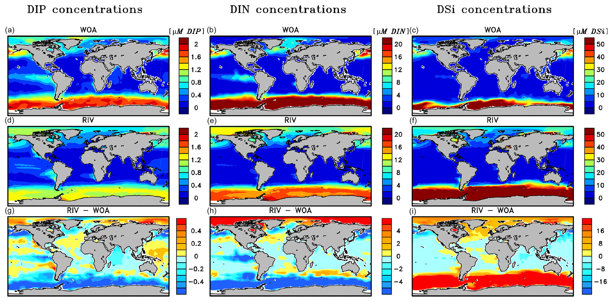
Figure 4Surface DIP (a, d, g), DIN (b, e, h) and DSi (c, f, i) concentrations in WOA observations (a, b, c), RIV (d, e, f) and their differences RIV-WOA (g, h, i).
4.2 Riverine-induced NPP hotspots
The open ocean regions with the highest NPP rates in REF remain the most dominant areas of NPP in RIV (Fig. 5a, b), which also confirms the major importance of the ocean physics in dictating spatial patterns of the global NPP. In comparison to REF, substantial enhancements of the NPP are simulated near major river mouths in RIV. In proximity to river mouths in lower latitudes, the uptake of nutrients by the phytoplankton occurs efficiently due to favorable light conditions, thus adding to the local organic matter stock (Fig. 5c, d). This can be observed on the shallow shelves of the western tropical Atlantic, where major nutrient supplies are provided (see Sect. 3.3). Moreover, the NPP is increased in certain semi-enclosed seas such as the Caribbean Sea, the Baltic Sea, the Black Sea and the Yellow Sea, where satellite observational data also suggest high chlorophyll concentrations (Behrenfeld and Falkowski, 1997).
In the tropical Atlantic, tropical Pacific, North Pacific and Southern Ocean, the NPP is decreased in RIV with respect to REF, signaling that stabilizing ocean biogeochemical inventories with open ocean inputs, as was done in REF, also led to a slight artificial enhancement of the NPP in these regions. The decrease in the equatorial Pacific could partly be explained by the characteristics of South American river systems, which almost solely debouch into the Atlantic basin (Fig. 7). Although Southeast Asian rivers deliver substantial biogeochemical loads to the ocean, the export of the biogeochemical compounds from eastern Asian coastal systems to the open Pacific is likely inefficient, with modeled salinity profiles of the East China Sea suggesting little mixing with the open ocean (Supplement S4). Currents parallel to the coast could be a key reason explaining this inefficient export (Ichikawa and Beardsley, 2002). The decrease in the equatorial Pacific NPP is also likely responsible for most of the shrinking of the global oxygen minimum zone volume (Table 5).
The Arctic Ocean does not undergo a noticeable increase in NPP, despite high nutrient concentrations in the basin in RIV. This can be explained by the region's light limitation over most of the year, as well as the presence of sea ice coverage, which both inhibit the primary production especially during winter. In the entire basin, the nutrient concentrations are much higher than what is suggested in the WOA database. In Bernard et al. (2011), where riverine nutrient inputs were added to the ocean according to the NEWS2 study, similarly high concentrations of DSi were found in the Arctic. Furthermore, Harrison and Cota (1991) suggest that in the Arctic Ocean, nutrients limit phytoplankton growth in the late summer. Although the Arctic NPP in RIV and REF is substantially higher in the summer than in other seasons, the NPP is never nutrient limited for the vast majority of the ocean basin.
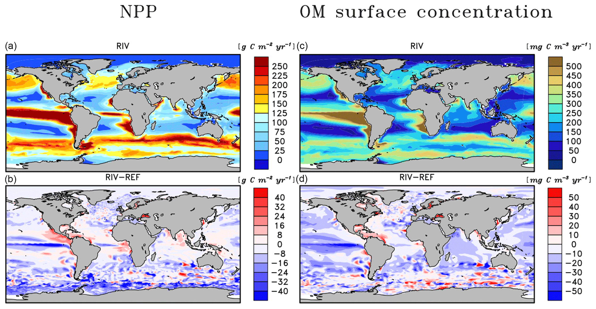
Figure 5Depth integrated annual NPP (a, b) and total annually accumulated organic matter concentration (c, d) in the surface layer in the RIV simulation and RIV – REF.
4.3 Riverine-induced CO2 Outgassing
The addition of riverine C loads causes a simulated net oceanic CO2 source of 231 Tg C yr−1 to the atmosphere (Table 5). While the hotspots of the riverine-induced C outgassing are regions in proximity to major river mouths (Fig. 6b), a widespread, albeit weaker, outgassing signal can be observed in open ocean basins. The largest outgassing fluxes are found in the Atlantic and Indo-Pacific (31 % and 43 % of global outgassing flux respectively), which is due to large riverine C supplies from tropical Atlantic and Southeast Asian catchments (see Sect. 3.2). In the Southern Ocean, we observe an outgassing flux of 17 Tg yr−1 when comparing RIV to REF, which is almost 10 % of the global riverine-caused outgassing. The riverine-induced outgassing is 113 Tg yr−1 (49 % of the global outgassing flux) in the Southern Hemisphere, despite riverine C exports of the hemisphere contributing to only 199 Tg (33 %) of annual C loads to the ocean. This implies the presence of an oceanic interhemispheric transfer of riverine C from the Northern Hemisphere to the Southern Hemisphere (Fig. 6c). This interhemispheric transfer of C in the ocean has been a topic of discussion in literature, with studies of Aumont et al. (2001) and Resplandy et al. (2018) also suggesting a transport of C between latitudinal regions of the ocean that compensates for the heterogeneous distribution of riverine C inputs.
The Arctic rivers (Lena, Mackenzie, Yenisei, Ob, Oder, Yukon) also provide C to their respective shelves, which causes a net outgassing of riverine C on the Laptev shelf and in the Beaufort Sea (2.2 and 2.3 Tg C yr−1, respectively). The impacts of riverine C loads on the Arctic shelves can also be observed in the present-day coastal ocean pCO2 data set of Laruelle et al. (2017), in which very high pCO2 values are reported near river mouths (> 400 ppm).
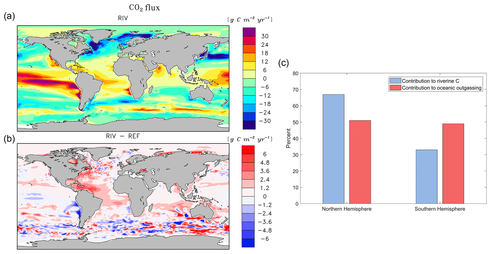
Figure 6Annual pre-industrial air–sea CO2 flux of (a) RIV, (b) RIV-REF, and (c) contributions of the Northern Hemisphere and Southern Hemisphere to riverine C loads and oceanic riverine C outgassing. A positive flux in (a) and (b) describes an outgassing flux from the ocean to the atmosphere, whereas a negative flux is a flux from the atmosphere to the ocean.
With respect to the 10 shallow shelf regions chosen for this study (Table 1), the catchments of the low latitude regions (5 CSK, 6 BEN, 7 SEA, 8 TWA, 9 CG) provide substantially more C and nutrients to the coastal ocean than the high latitude regions in our framework (Fig. 7), although the differing size of the coastal regions and of their catchments may play a strong role in explaining these differences. The tropical west Atlantic (8 TWA) has the largest riverine supplies of biogeochemical compounds, which are largely provided by the Amazon and Orinoco rivers. In the tropical regions of the Bay of Bengal (6 BEN) and Southeast Asia (7 SEA), the fraction of C delivered as POC is substantially higher than for the rest of the regions (Fig. 7b). Furthermore, in the high latitude regions (1 BS, 2 LS, 3 NS, 10 SAM), DIC loads are the major source of riverine C, whereas for the other regions, organic C is the largest contributor to the regional C load. The higher importance of DIC loads for the Arctic C supplies can also be observed in Table 4.
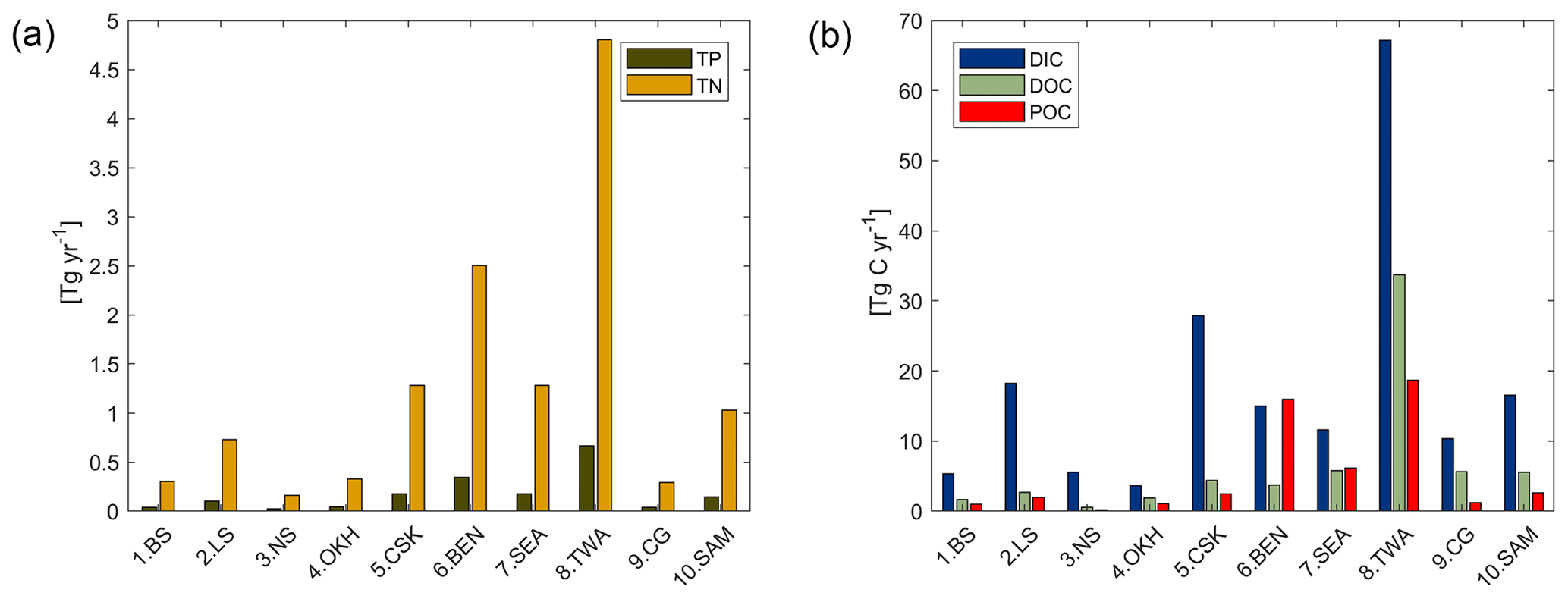
Figure 7Modeled riverine (a) P (TP) and N (TN), and (b) C (DIC, DOC and POC) exports to selected coastal regions. TP and TN are the total P and N from the sum of their riverine dissolved inorganic loads (DIP, DIN) and of their riverine organic loads (P and N within tDOM and POM). DOC and POC are the C loads within riverine tDOM and POM, respectively.
In RIV, major coastal ocean NPP increases of 166 %, 377 % and 71 % for the tropical west Atlantic (3 TWA), Bay of Bengal (5 BEN) and East China Sea (6 CSK), respectively, are simulated, in comparison to REF (Fig. 8b). The availability of light, as well as the large riverine supplies of nutrients to these regions (Table 4 in Sect. 3.2), provides optimal conditions to enhance the biological production. Surprisingly, the Southeast Asian shelf (6 SEA) does not undergo a large relative increase in its regional NPP despite considerable riverine inputs to the region and favorable climatic conditions for biological production in the region. This, on the one hand, is due to the large area of the defined region (1795×109 m2), which reduces the impact of the riverine loads per area. On the other hand, there is a larger connection area to the open ocean due to not sharing a coastal border with a continent, which implies a larger open ocean exchange, thus the influence of the riverine supplies is likely to be less significant than contributions from open ocean supplies. In turn, the Congo shelf (9 CG) has a very small surface area (53×109 m2) due to a steep coastal slope (Supplement S4). The NPP in the region is however already one of the highest of the chosen regions in REF, indicating that the region is already strongly supplied with nutrients from open ocean inflows. The relative impact caused by the addition of riverine inputs is therefore minor.
On the temperate shelf regions, where a stronger seasonal cycle of the light limitation takes place, the NPP in the North Sea (2 NS) is only weakly enhanced when comparing RIV to REF (+2 %). In the South American (10 SAM) and Sea of Okhotsk (4 OKH) regions substantial NPP increases due to the addition of riverine inputs are also not simulated. Although the NPP is strongly enhanced in the direct proximity to the Paraná river (Fig. 5b), the vastness of the South American shelf (1553×109 m2) also makes the region less sensitive to riverine inputs. In published literature, the nutrient supply which drives the NPP on the Patagonian shelf is also confirmed to be strongly controlled by open ocean inflows, and river supplies are suggested to only have a limited influence in the region (Song et al., 2016).
The Arctic shelf regions also do not undergo a strong NPP increase in RIV with respect to REF (8 % and 5 % increases for the Beaufort Sea, 1 BS, and Laptev Sea, 2.LS, respectively). We however do not consider a seasonality of the riverine inputs. Larger inputs of nutrients in months of larger discharge from April to June (Le Fouest et al., 2013) could cause a more efficient usage of the riverine nutrients on the shelves, since the light availability is higher and the sea ice coverage is reduced during these months.
An increase in CO2 outgassing due to the increased C inputs is simulated in all regions in RIV. In the Arctic regions (Beaufort Sea and Laptev Sea), the relative change in the air–sea CO2 flux is very pronounced, whereas the impact is generally not as strong in the lower latitude regions due to the enhancement of the biological DIC uptake caused by riverine nutrient inputs. The tropical west Atlantic is an exception to this latitudinal pattern, since the large riverine C supplies also cause a substantial change in the CO2 flux of the region. In the North Sea, we observe an enhancement of C outgassing induced by riverine loads, but the region remains a substantial pre-industrial sink of atmospheric CO2 in RIV, as is still suggested for the present day by Laruelle et al. (2014).
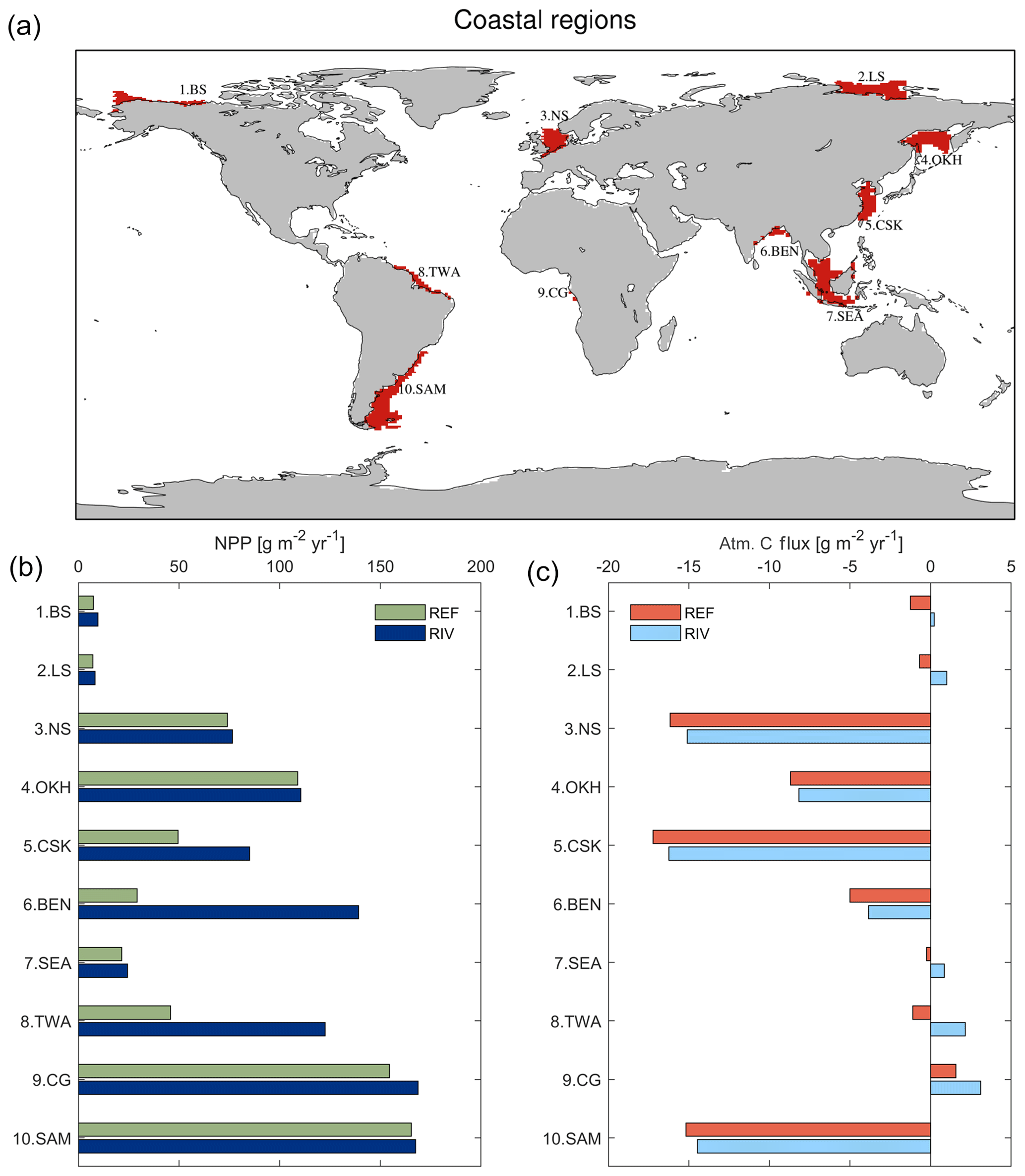
Figure 8(a) Global map of the 10 chosen coastal regions with depths of less than 250 m, (b) pre-industrial annual NPP per area and (c) CO2 flux in the given regions (g C m2 yr−1). In (c), a positive flux means a flux from the ocean to the atmosphere.
In our simplified model framework (Fig. 9), we quantify the land sources of riverine C (1–3), its riverine transfer to the ocean (4) and the long-term fate of the riverine C in the ocean (5–10). While the terrestrial fluxes are derived from the weathering and organic matter export models, the fluxes of the riverine C in the ocean are derived from RIV–REF differences of the ocean simulation. The long-term oceanic CO2 flux is furthermore decomposed to illustrate the contributions of riverine inorganic and organic C inputs to the oceanic outgassing flux in a model equilibrium analysis. The detailed calculations of the land and ocean fluxes are shown and explained in detail in the Appendix C (C1 for terrestrial and C2 for oceanic fluxes).
In our framework, the global pre-industrial terrestrial uptake of atmospheric C and its export to rivers as DIC amounts to 529 Tg C yr−1. The sink consists of 280 Tg C yr−1 from the drawdown induced by weathering (1) and of 249 Tg C yr−1 from the terrestrial biological uptake (3). During the weathering process, 94 Tg C yr−1 is moreover released from the lithology through carbonate weathering (2). During silicate weathering, all the C released originates from atmospheric CO2. The terrestrial biological uptake (3) is derived from the net global export of organic C to the ocean. It therefore implicitly takes into account the net land biological uptake and its export to freshwaters, as well as all net sinks and sources in river systems. A total of 603 Tg C yr−1 is transferred laterally to the ocean (4) while taking into consideration an endorheic catchment loss of 19 Tg C yr−1.
In the ocean, riverine inputs of C cause a long-term net annual atmospheric source of 231 Tg C yr−1 (Table 5). We propose a decomposition of this long-term CO2 flux into sources and sinks induced by the inputs of the riverine compounds (Appendix C2). Assuming model equilibrium, the oceanic outgassing flux can be decomposed into a source from riverine inorganic C inputs (183 Tg C yr−1, 5), a source from terrestrial organic C (128 Tg C yr−1, 6) and a sink caused by the enhancement of the biological production prompted by the addition of dissolved inorganic nutrients and its associated alkalinity production (69 Tg C yr−1, 7). We also calculate a sink due to disequilibrium at the atmosphere–water column interface in the model (11 Tg C yr−1, Dr1). The production and the downwards export of CaCO3 and POM within the ocean lead to simulated sediment deposition fluxes of 188 Tg C yr−1 for CaCO3 (inorg. C flux, 8) and of 582 Tg C yr−1 for POM (org. C flux, 9). The dissolution of CaCO3 and the remineralization of POM within the sediment lead to a DIC flux of 385 Tg C yr−1 from the sediment pore water to the water column. The net C flux at the sediment interface () is therefore a burial flux of 385 Tg C yr−1. The calculated equilibrium C burial flux, which is the difference between the riverine C inputs and the equilibrium CO2 outgassing (), is 361 Tg C yr−1, which implies that there is a deviation of 24 Tg C yr−1 (Dr2) towards the sediment. With the simulated C burial (385 Tg C yr−1) deviating from the calculated equilibrium state C burial (361 Tg C yr−1). Similar deviations from the equilibrium states at the atmosphere–water column and water column–sediment interfaces suggest that the model disequilibrium, which is likely due to the long timescales of the processes taking place in the sediment, translates relatively efficiently into a perturbation of the CO2 flux at the atmosphere–water column interface.
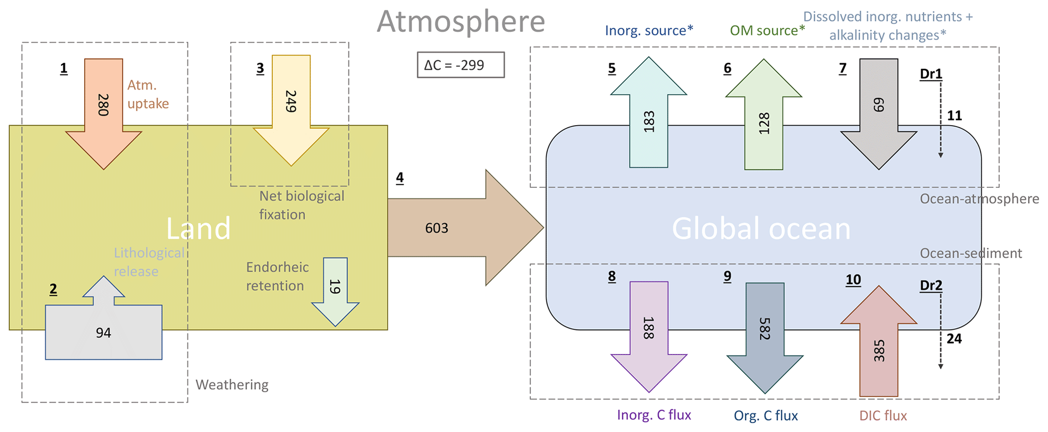
Figure 9Origins and oceanic fate of riverine C in our framework (Tg C yr−1). (1) Atmospheric C uptake through weathering. (2) Carbonate weathering C flux from the lithology. (3) Net land biological C uptake (derived directly from riverine organic C exports). (4) Total riverine C exports. (5) Oceanic C outgassing from riverine DIC (i.e., inorganic C) inputs. (6) Oceanic C outgassing resulting from riverine tDOM inputs. (7) Oceanic C uptake due to the enhanced primary production by dissolved inorganic nutrients and the corresponding alkalinity production. (8) Simulated inorganic C deposition (i.e., CaCO3 to the sediment. (9) Simulated net organic C (i.e., POM) deposition to sediment. (10) Diffusive DIC flux from the sediment pore water back to the water column. Given are simulated fluxes by the terrestrial and ocean models, except when * is stated, meaning that the fluxes were calculated assuming model equilibrium. Dr1 and Dr2 are the calculated drifts between the simulated oceanic C fluxes and the calculated equilibrium fluxes (derived from model equations, Appendix C2) for the ocean–atmosphere and ocean–sediment interfaces, respectively. See Appendix C for the calculation of all fluxes.
The simulated riverine-induced oceanic CO2 outgassing flux of 231 Tg C yr−1 is consistent with the estimate range of 200–400 Tg C yr−1 given in Sarmiento and Sundquist (1992), who derived an annual global riverine C load of 300–500 Tg C, and with Jacobson et al. (2007) and Gruber et al. (2009), who suggest a slightly higher natural CO2 outgassing flux of 450 Tg C yr−1. A recent study by Resplandy et al. (2018) proposes both riverine C loads and oceanic C outgassing of 780 Tg C yr−1. It is however unclear if and how the oceanic carbon removal of the riverine C through sediment burial was considered in the study.
Furthermore, we observe an imbalance in the calculated pre-industrial land uptake and the oceanic outgassing of atmospheric CO2 in our approach, with the land uptake outweighing the oceanic outgassing (combined net atmospheric sink of 299 Tg C yr−1). Accounting for further sources of atmospheric CO2 such as volcanic emissions and shale oxidation would therefore be necessary to achieve a stable atmospheric carbon budget in a fully coupled land–ocean–atmosphere setting, since ESMs assume constant pre-industrial atmospheric CO2 levels. For instance, Mörner and Etiope (2002) suggest long-term volcanic annual emissions in the range of 80–160 Tg C yr−1, whereas Burton et al. (2013) estimate a long-term volcanic outgassing flux as high as that of silicate weathering drawdown. In our approach, the modeled silicate weathering CO2 drawdown is 196 Tg C yr−1. Additionally to the volcanic CO2 emissions, the global atmospheric CO2 land source from the oxidation of organic carbon in shale of around 100 Tg C yr−1 given by Sarmiento and Sundquist (1992) would then be approximately close the atmospheric carbon budget in our framework.
7.1 Rivers in an Earth system model setting
Our approach, which quantifies riverine exports as a function of the climate variables precipitation, surface runoff and temperature can potentially be used to estimate land–ocean exports in an ESM setting. Since we establish a baseline for the pre-industrial state of the ocean while considering riverine loads, our study could also be used to assess oceanic impacts of perturbations of riverine loads due to temporal changes in weathering rates (Gislason et al., 2009), or due to increased anthropogenic P and N inputs to catchments (Seitzinger et al., 2010; Beusen et al., 2016).
This study however also relies on strong assumptions in order to perform simulations at the global scale, although improvements within the framework are possible. For one, the weathering mechanisms, the processing uptake of nutrients by the terrestrial biology, the representation of hydrological flow characteristics, as well as transformation processes and retention in rivers could all be represented more realistically. We notably assumed a fixed riverine N:P mole ratio of 16:1 for all species and all catchments in this study. Riverine N:P ratios are suggested to exceed this ratio at the global scale (29:1 by Seitzinger et al., 2010 and 21:1 by Beusen et al., 2016), but denitrification in estuaries could compensate the excess of N with regard to a N:P ratio of 16:1 (see Supplement S1.3). Denitrification in estuaries is impossible to represent in the ocean model due to grid resolution constraints. Furthermore, we assume a similar spatial distribution of pre-industrial anthropogenic P inputs as for the present day. While the chosen spatial distribution agrees well with the distribution of other approaches (Supplement S1), we acknowledge a large degree of uncertainty both in the magnitudes of the pre-industrial anthropogenic inputs as well as in their distributions.
7.2 Dynamics of terrestrial organic matter in the ocean
The composition of terrestrial organic matter and its fate in the ocean have been strongly debated in the past. Recent work shows that despite its low biological reactivity, tDOM can be mineralized by abiotic processes such as photodegradation in the ocean (Fichot and Benner, 2014; Müller et al., 2016; Aarnos et al., 2018), despite already having been strongly degraded during its transit in rivers. The global magnitude of the degradation of tDOM in the ocean is however strongly uncertain. Few studies in the past have addressed the composition of POM, although it is also thought to be efficiently remineralized in the coastal ocean sediment (Hedges et al., 1997; Cai, 2011). While the C loads from POM are the lowest loads of all C compounds considered in this study, a differing C:P ratio to the one chosen in this study could affect the modeled riverine-induced C outgassing flux in the ocean.
Rates of remineralization processes have been suggested to be higher in the coastal ocean than in the open ocean (e.g., Krumins et al., 2013). Using a higher coastal organic matter remineralization rate in the sediment module of HAMOCC could potentially reduce the coastal biogeochemical sink described in this study and increase the offshore export of biogeochemical compounds.
7.3 Arctic Ocean
Simulated nutrient concentrations are particularly high in the Arctic Ocean with regard to WOA data, suggesting that this region with strong riverine inputs might be poorly represented in the HAMOCC. Difficulties to represent the region could be due to fine circulation features. For instance, outflows through narrow passages have been shown to be affected by model resolution (Aksenov et al., 2010). The simulated sea ice coverage in our study, which is around 85 % for the Laptev Sea during the whole year on average, could be overestimated. Moreover, the NPP in the region might be underestimated due to photosynthesis taking place under ice, in ice ponds and over extended daytime periods in the summer months (Deal et al., 2011; Sørensen et al., 2017), all of which are not represented in HAMOCC.
In this study, we account for weathering and non-weathering inputs to river catchments to quantify global annual pre-industrial loads of 3.7 Tg P, 27 N, 168 Tg DSi and 603 Tg C to the ocean. These loads are consistent with published literature estimates, although we acknowledge a certain degree of uncertainty regarding their magnitudes. While we omit the in-stream retention of P during its riverine transport, which reduces the global P exports to the ocean (Beusen et al., 2016), our estimate of the global pre-industrial P export to the ocean is comparable in magnitude to an estimation that determines riverine P exports by upscaling from pristine river measurements (Compton et al., 2000).
We identify the tropical Atlantic catchments, the Arctic Ocean, Southeast Asia and Indo-Pacific islands as regions of dominant contributions of riverine supplies to the ocean. These four regions account for over 51 % of land–ocean C exports in total, with tropical Atlantic catchments supplying around 20 % of C to the ocean globally. We also observe that the contributions of different C species differ between the regions. Most prominently, the C supply of the Indo-Pacific islands is dominated by particulate organic C loads, which have been identified to be more strongly controlled by extreme hydrological events than other C species (Hilton et al., 2008).
In the ocean model, riverine inputs of C lead to a net global oceanic outgassing flux of 231 Gt C yr−1, a comparable value with regards to previous estimates of 200–450 Tg C yr−1 (Sarmiento and Sundquist, 1992; Jacobson et al., 2007; Gruber et al., 2009). This outgassing flux can be decomposed into two source terms caused by inorganic C inputs (183 Tg C yr−1) and organic C inputs (128 Tg C yr−1), and a net sink term (80 Tg C yr−1) caused by the enhanced biological C uptake due to riverine inorganic nutrient supplies, corresponding alkalinity production and a slight model drift in alkalinity. The magnitude of the outgassing is however strongly dependent on the magnitude of riverine C loads. In our framework, both riverine C loads and their induced oceanic C outgassing are thereby situated within the lower range of estimates.
We find evidence of a substantial oceanic interhemispheric transport of riverine C from the Northern Hemisphere to the Southern Hemisphere, with a larger relative C outgassing flux simulated over the Southern Hemisphere (49 % of global outgassing) than its relative riverine C loads (36 % of global C loads). We also show that the Southern Ocean outgasses 17 Tg of riverine C, despite not having a direct riverine source of C, meaning that riverine C is transported within the ocean interior to the Southern Ocean in the model. This interhemispheric transfer of riverine C in the ocean has previously been suggested to contribute to the pre-industrial Southern Ocean source of atmospheric CO2 for the pre-industrial time frame (Sarmiento et al., 2000; Aumont et al., 2001; Gruber et al., 2009; Resplandy et al., 2018). Here, we show that riverine C exports derived from state-of-the-art land export models confirm the larger contribution of the Northern Hemispheric terrestrial C supply to the ocean. Part of this uneven terrestrial C supply is then compensated by the transport of C within the ocean and is outgassed remotely.
Our results help identify oceanic regions that are sensitive to riverine fluxes. Riverine-induced changes in the regional NPP are mostly found in coastal regions, but substantial riverine-caused CO2 outgassing can also be observed in the open ocean of the tropical Atlantic. In general, we show latitudinal differences in the sensitivity of the NPP and of the CO2 fluxes to the riverine inputs in various coastal regions. While a high sensitivity in the NPP is found in the tropics and subtropics, with the tropical west Atlantic, the Bay of Bengal and the East China Sea showing large NPP increases of 166 %, 377 % and 71 %, respectively, the relative changes in the regional CO2 fluxes are mostly larger at higher latitudes. For instance, the Laptev Sea and the Bay of Beaufort become atmospheric sources of 2.2 and 2.3 Tg C yr−1 respectively, despite being sinks of atmospheric CO2 without accounting for riverine inputs. While our analysis revolves around the implications of pre-industrial riverine loads, regions that show strong responses to the riverine loads in this study might also be strongly affected by anthropogenic perturbations of riverine exports.
Deriving riverine exports as a function of ESM variables enables a representation of the riverine loop; starting from the terrestrial uptake of C to its riverine export and ending with its long-term outgassing in the ocean or export to the oceanic sediment. In order to implement the framework into a coupled land–atmosphere–ocean setting such as an ESM, the atmospheric pre-industrial budget would have to be balanced. We emphasize the need to consider long-term terrestrial CO2 sources originating from long-term volcanic activity and from shale oxidation in order to compensate for imbalances between the terrestrial C sink and the oceanic C source in our framework.
Throughout this study, we find global heterogeneity in the spatial features of weathering fluxes, riverine loads and their implications for the ocean biogeochemistry. We confirm that considering riverine exports to the ocean is central when assessing the biogeochemistry of coastal regions, but also find implications for certain open ocean regions (i.e., the tropical Atlantic). Our study also shows the necessity to account for the river-induced oceanic C outgassing in ocean biogeochemistry models, since our conservative estimate consists of around 10 % of the magnitude of the present-day oceanic C uptake.
Code, primary data and scripts needed to reproduce the analyses presented in this study are archived by the Max Planck Institute for Meteorology and are available upon request (publications@mpimet.mpg.de).
The supplement related to this article is available online at: https://doi.org/10.5194/bg-17-55-2020-supplement.
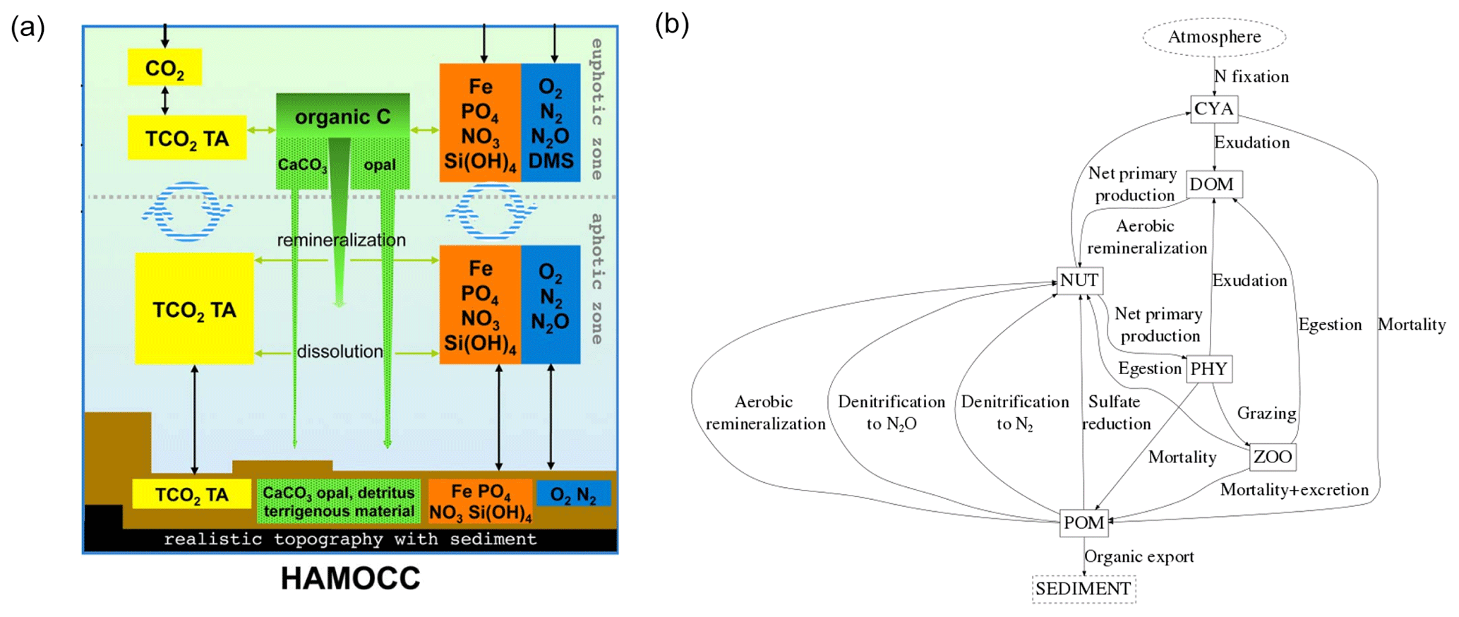
Figure A1(a) Scheme of model compartments in HAMOCC, modified from Ilyina et al. (2013) and (b) scheme of the organic dynamics taking place in the model. The most central model parameters can be found in the Supplement S2.
The weathering yields provided in this study are dependent on the MPI-ESM spatial representation of pre-industrial surface runoff, surface temperature and precipitation (Fig. B1a, b, c).
Previous work by Goll et al. (2014) describes the MPI-ESM performing well when estimating surface temperatures at single grid cells with regard to observations. The global precipitation in MPI-ESM is slightly higher than the global precipitation that is reported in the Global Precipitation Climatology Project (GCPC) (Adler et al., 2003), which is discussed along with spatial biases of the precipitation in Stevens et al. (2013). Most notably, the precipitation is too strong over extratropical land surface and too little over tropical land surface. Runoff is less well reproduced globally. For the given time period of the simulation used in this study, the global runoff is 23 496 km3 yr−1. This is significantly lower than the global runoff estimations of 36 600–38 300 km3 yr−1 (Fekete et al., 2002; Dai and Trenberth, 2002). The difficulty of representing several processes that control the runoff, such as evapotranspiration and condensation, is also reflected in the large range of global runoff means of other Earth system models, which range from 23 000 to 42 500 km3 yr−1 (Goll et al., 2014).
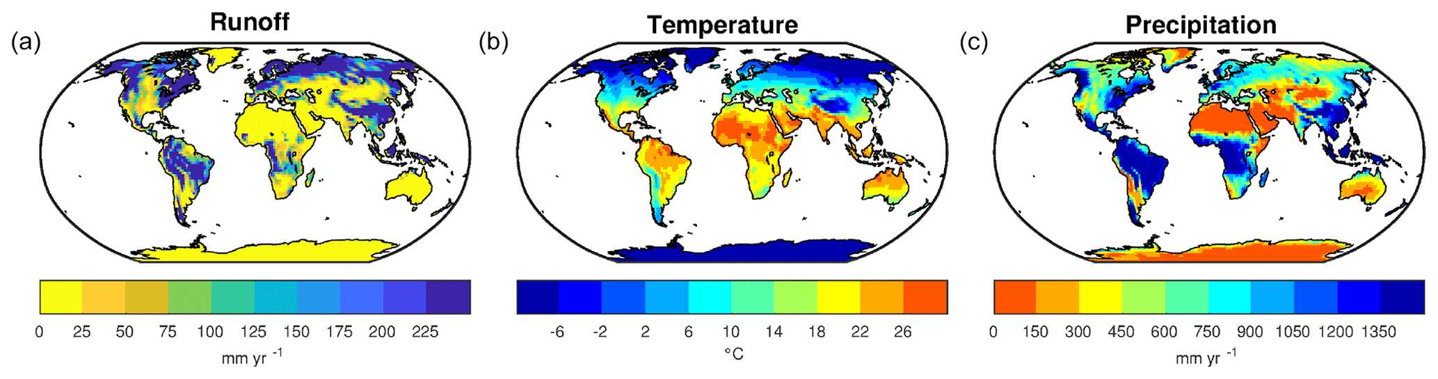
Figure B1Modeled pre-industrial (a) surface runoff (mm a−1), (b) surface temperature (∘C) and (c) precipitation (mm a−1) annual means.
The spatial patterns in the CMIP5 simulation are however comparable with the annual runoff patterns reported in Fekete et al. (2002), with high surface runoff observed in the Amazon basin, West Africa, Indo-Pacific islands, Southeast Asia, eastern North America, northern Europe as well as in Siberia. Due to the strong underestimation of the model regarding the runoff in relation to the combined runoff mean of Fekete et al. (2002) and Dai and Trenberth (2002), we conclude that a scaling factor of 1.59 is necessary to represent runoff plausibly at the global scale. The global runoff from OMIP, which provides freshwater to the ocean model, is however more plausible (32 542 km3 yr−1) and was therefore not scaled. We scaled the model runoff to the global runoff estimation from Fekete et al. (2002) and not to the OMIP runoff, since scaling to the OMIP runoff still led to lower global P and DIC:Alk release values than were reported in literature estimates.
C1 Terrestrial fluxes
-
Carbonate and silicate weathering cause a terrestrial uptake of 280 Tg C yr−1 from the atmosphere according to the weathering model simulations (Table 2).
-
Carbonate mineral weathering causes a lithological C release flux of 94 Tg C yr−1 DIC, as shown in Sect. 3.2.
-
Carbon contained in terrestrial organic matter exports originates from the atmosphere (Meybeck and Vörösmarty, 1999). The net C uptake by the terrestrial and riverine biology is therefore the same as the lateral organic C export, which we derived from NEWS2 (Seitzinger et al., 2010) DOC and POC exports. The net atmospheric C uptake by the terrestrial biology, while taking into account all respiration processes on land and in rivers, is the sum of the lateral POC and DOC exports (249 Tg C yr−1).
-
The global riverine C export to the ocean consists of the sum of weathering and organic matter C exports (623 Tg C yr−1) minus a loss term due to endorheic river retention (19 Tg C yr−1). This results in the global riverine C export of 603 Tg C yr−1 (values are rounded).
C2 Long-term ocean fluxes
In the model, riverine loads cause oceanic C outgassing due to the inputs of inorganic C and tDOM, while the inputs of dissolved inorganic nutrients cause a sink of atmospheric C through their enhancement of the biological C uptake. Increased primary production thereby also produces alkalinity, which also potentially causes an uptake of atmospheric C.
Inorganic C is delivered to the ocean by rivers as 1 mol DIC and 1 mol alkalinity, which represent the supply of , and it is exported from the ocean as CaCO3, which accounts for 0.5 mol DIC per 1 mol alkalinity, leaving a surplus of 0.5 mol DIC and 0 mol alkalinity when balancing over the oceanic inputs and exports. Increasing the oceanic DIC pool without increasing the alkalinity directly increases the dissolved CO2 concentrations, which in turn causes outgassing:
Equilibrium model outgassing caused by riverine inorganic C inputs is therefore 0.5 fold of the riverine DIC loads.
Outgassing from organic matter inputs results from the high C:P ratio of tDOM. tDOM, in contrary to POM, is not exported to the sediment. It is mineralized in the ocean, providing dissolved inorganic compounds in the ratio of , but the subsequent uptake of the released inorganic compounds happens at a ratio of , resulting in a DIC overshoot. Since the net alkalinity over the entirety of Eq. (C2) is also constant, the DIC increase causes a pCO2 increase (* simplified equation):
The organic outgassing caused by organic matter inputs is therefore 2461:2583 multiplied with tDOM carbon loads.
The riverine loads of DIP and DIN on the other hand cause C uptake through their enhancement of the biological primary production. DIC:CO2 is thereby removed, thus sinking pCO2 (* simplified equation):
The resulting C uptake from the equation is therefore 122-fold the mole DIP inputs. Additionally, alkalinity is produced in Eq. (C3). The uptake of DIN (assuming nitrate and not ammonium,as is done in HAMOCC) and DIP through primary production causes a net alkalinity increase by a factor of (Wolf-Gladrow et al., 2007). In model equilibrium, the produced alkalinity must also be exported through Eq. (C1). This alkalinity is exported in a C:Alk ratio of 1:2, meaning an uptake of 0.5 DIC per mol alkalinity exported. The C uptake enhancement from the alkalinity increase is therefore the 17×0.5 multiplied with the (bioavailable) DIP loads.
With the help of these equations, the fluxes of riverine C in the ocean of Fig. 9 were calculated.
- 5.
According to the CaCO3 export equation (Eq. C1), half of the riverine DIC input is exported to the sediment as CaCO3, and the other half is outgassed as CO2 in model equilibrium state. The contribution of outgassing caused by inorganic C in the ocean is therefore 0.5-fold the DIC inputs (366 Tg C yr−1) and therefore 183 Tg C yr−1 assuming model equilibrium.
- 6.
tDOM input C:P rations vastly exceed the oceanic sediment export C:P ratios of organic matter, which causes model equilibrium outgassing in the ocean. Equation (C2) shows that for every mol tDOM supplied to the ocean, in model equilibrium 122:2583 of C is exported to the sediment, and 2461:2583 of C increases the dissolved CO2 pool, which is outgassed in the long term. The equilibrium outgassing is therefore the tDOM carbon load (134 Tg C yr−1) multiplied by 2461:2583, which results in 128 Tg C yr−1. In the case of POM, since the C:P ratio of the riverine input (122:1) is the same as the ratio of the export to the sediment in the ocean, there is no effect on the long-term equilibrium C outgassing flux.
- 7.
Since P has no further sinks or sources in the model other than riverine inputs and sediment burial as organic matter, in model equilibrium the same amount of P supplied by rivers is buried in the sediment. When DIP is taken up by the biology and transformed to organic matter, carbon is also taken up in a mole ratio of . Accounting for this uptake through the biological production enhancement by DIP inputs (including all bioavailable DIP) from rivers (1.4 Tg P yr−1) results in the uptake of 67 Tg C yr−1 through the biological enhancement. Furthermore, when DIP and DIN are transformed to organic matter, an alkalinity increase of 17 mol mol−1 DIP uptake takes place (Eq. C3, Wolf-Gladrow et al., 2007). This increase in alkalinity causes the further uptake uptake and export of 2 Tg C yr−1, resulting in a total sink of 69 Tg C yr−1.
- Dr1.
We attribute the difference between the equilibrium CO2 flux of 242 Tg C yr−1 and the modeled net CO2 flux of 231 Tg C yr−1 (=11 Tg C yr−1) to the small surface alkalinity increase in the model simulations due to slight disequilibrium over the analysis time period.
- 8.
The simulated global particulate inorganic C sediment deposition flux in HAMOCC is 188 Tg C yr−1.
- 9.
The simulated global organic C sediment deposition flux in HAMOCC model is 582 Tg C yr−1.
- 10.
The modeled global DIC flux from the sediment back to the water, which originates from DIC release due to POM remineralization and CaCO3 dissolution in the sediment, is 385 Tg C yr−1.
- Dr2.
In model equilibrium, the net sediment burial C flux is the total riverine C inputs of 603 Tg C yr−1 (4) subtracted by the equilibrium outgassing of 242 Tg C yr−1 (), which results in 361 Tg C yr−1. The simulated net C burial flux in the simulations of 385 Tg C yr−1 () deviates from the calculated model burial equilibrium flux. Therefore, the drift at the sediment–ocean interface is 24 Tg C yr−1 (385–361 Tg C yr−1) and is in the direction of the sediment.
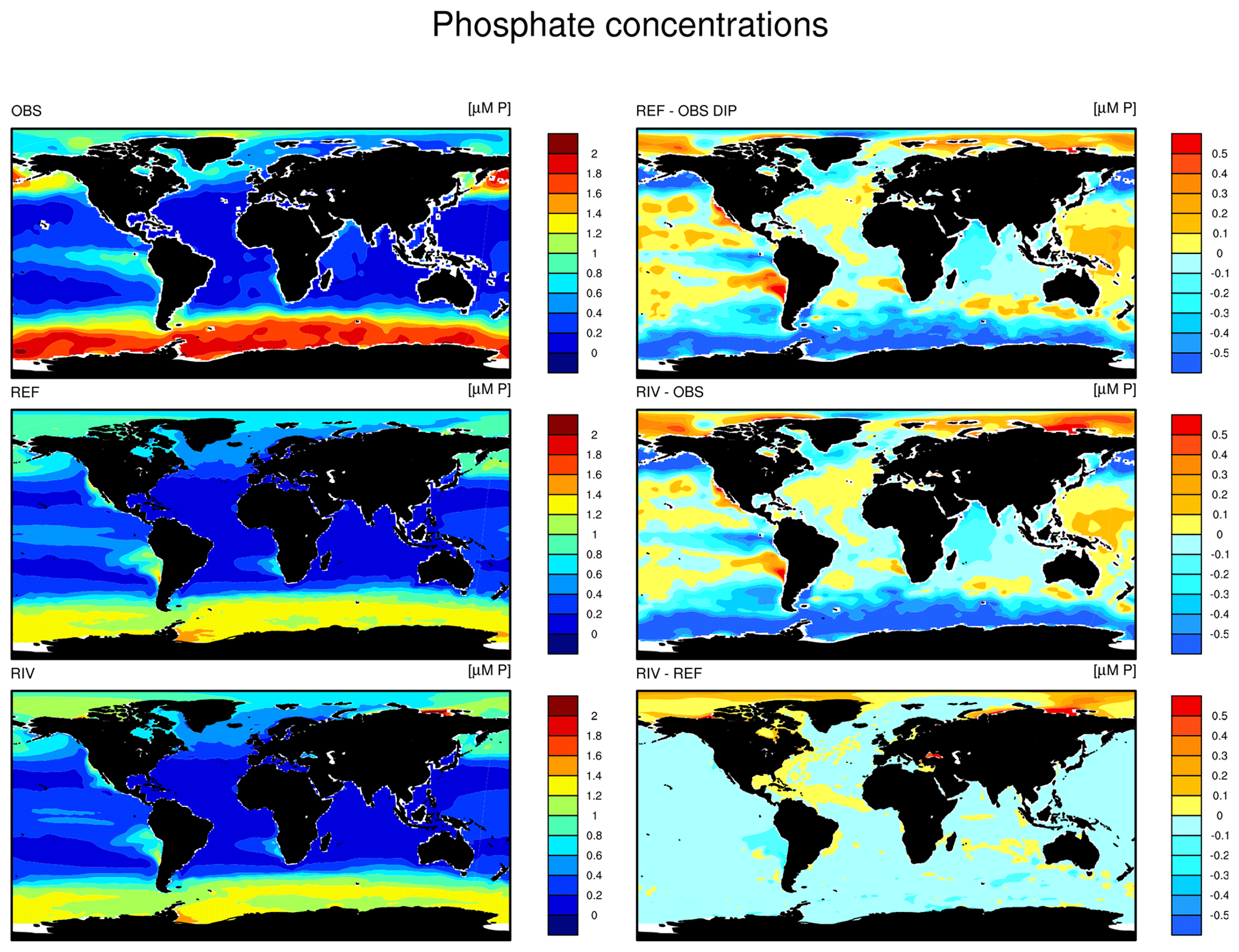
Figure D1DIP concentrations in OBS (WOA observations), REF and RIV.
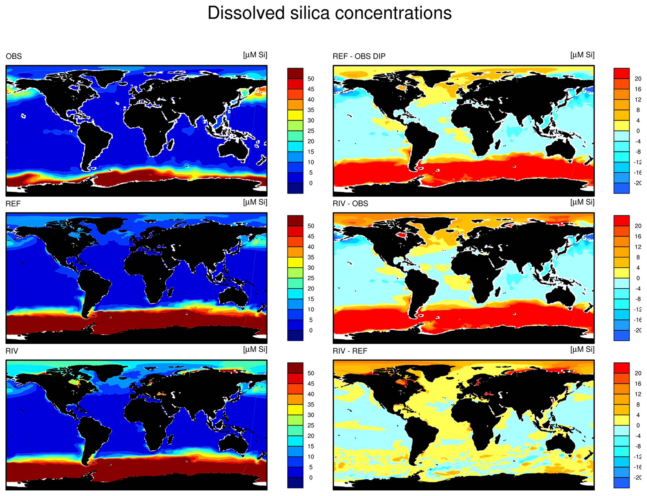
Figure D2Dissolved silica (DSi) concentrations in OBS (WOA observations), REF and RIV.
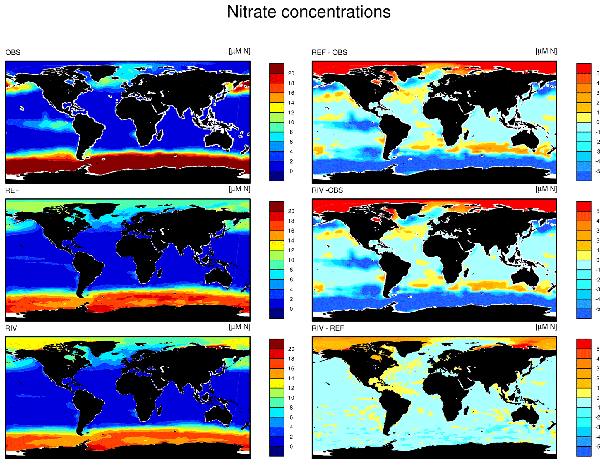
Figure D3Nitrate (DIN) concentrations in OBS (WOA observations), REF and RIV.
FL developed the model code, and performed the experiments. All co-authors contributed to the analysis and preparation of the manuscript.
The authors declare that they have no conflict of interest.
All simulations were performed at the German Climate Computing Center (DKRZ). The research leading to these results has received funding from the European Union's Horizon 2020 research and innovation program under the Marie Skłodowska-Curie grant agreement no. 643052 (C-CASCADES project). We acknowledge the constructive comments and suggestions received from Pierre Regnier, Irene Stemmler, Katharina Six and Philip Pika.
This research has been supported by the C-CASCADES (grant no. 643052).
The article processing charges for this open-access
publication were covered by the Max Planck Society.
This paper was edited by Jack Middelburg and reviewed by two anonymous referees.
Aarnos, H., Gélinas, Y., Kasurinen, V., Gu, Y., Puupponen, V.-M., and Vähätalo, A. V.: Photochemical Mineralization of Terrigenous DOC to Dissolved Inorganic Carbon in Ocean, Global Biogeochem. Cy., 32, 250–266, https://doi.org/10.1002/2017GB005698, 2018. a, b, c
Adler, R. F., Huffman, G. J., Chang, A., Ferraro, R., Xie, P.-P., Janowiak, J., Rudolf, B., Schneider, U., Curtis, S., Bolvin, D., Gruber, A., Susskind, J., Arkin, P., and Nelkin, E.: The Version-2 Global Precipitation Climatology Project (GPCP) Monthly Precipitation Analysis (1979–Present), J. Hydrometeorol., 4, 1147–1167, https://doi.org/10.1175/1525-7541(2003)004<1147:TVGPCP>2.0.CO;2, 2003. a
Aksenov, Y., Bacon, S., Coward, A. C., and Holliday, N. P.: Polar outflow from the Arctic Ocean: A high resolution model study, J. Marine Syst., 83, 14–37, https://doi.org/10.1016/j.jmarsys.2010.06.007, 2010. a
Amiotte Suchet, P. and Probst, J.-L.: A global model for present-day atmospheric ∕ soil CO2 consumption by chemical erosion of continental rocks (GEM-CO2), Tellus B, 47, 273–280, https://doi.org/10.1034/j.1600-0889.47.issue1.23.x, 1995. a, b, c, d, e, f, g
Amiotte Suchet, P., Probst, J.-L., and Ludwig, W.: Worldwide distribution of continental rock lithology: Implications for the atmospheric ∕ soil CO2 uptake by continental weathering and alkalinity river transport to the oceans, Global Biogeochem. Cy., 17, 1038, https://doi.org/10.1029/2002GB001891, 2003. a
Araujo, M., Noriega, C., and Lefèvre, N.: Nutrients and carbon fluxes in the estuaries of major rivers flowing into the tropical Atlantic, Front. Mar. Sci., 1, 1–16, https://doi.org/10.3389/fmars.2014.00010, 2014. a, b, c, d
Aumont, O., Orr, J. C., Monfray, P., Ludwig, W., Amiotte Suchet, P., and Probst, J.-L.: Riverinedriven interhemispheric transport of carbon, Global Biogeochem. Cy., 15, 393–405, https://doi.org/10.1029/1999GB001238, 2001. a, b, c, d, e
Batjes, N. H.: A world dataset of derived soil properties by FAO–UNESCO soil unit for global modelling, Soil Use Manage., 13, 9–16, https://doi.org/10.1111/j.1475-2743.1997.tb00550.x, 1997. a
Batjes, N. H.: Revised soil parameter estimates for the soil types of the world, Soil Use Manage., 18, 232–235, 2002. a
Behrenfeld, M. and Falkowski, P.: Photosynthetic rates derived from satellite-based chlorophyll concentration, Limnol. Oceanogr., 42, 1479–1491, https://doi.org/10.4319/lo.1997.42.1.0001, 1997. a
Benner, R., Louchouarn, P., and Amon, R. M. W.: Terrigenous dissolved organic matter in the Arctic Ocean and its transport to surface and deep waters of the North Atlantic, Global Biogeochem. Cy., 19, GB2025, https://doi.org/10.1029/2004GB002398, 2005. a
Bernard, C. Y., Dürr, H. H., Heinze, C., Segschneider, J., and Maier-Reimer, E.: Contribution of riverine nutrients to the silicon biogeochemistry of the global ocean – a model study, Biogeosciences, 8, 551–564, https://doi.org/10.5194/bg-8-551-2011, 2011. a, b, c
Berner, R. A., Lasaga, A. C., and Garrels, R.: The carbonate-silicate geochemical cycle and its effect on atmospheric carbon dioxide over the past 100 million years, Am. J. Sci., 283, 641–683, https://doi.org/10.2475/ajs.283.7.641, 1983. a, b
Beusen, A. H. W., Dekkers, A. L. M., Bouwman, A. F., Ludwig, W., and Harrison, J.: Estimation of global river transport of sediments and associated particulate C, N, and P, Global Biogeochem. Cy., 19, GB4S05, https://doi.org/10.1029/2005GB002453, 2005. a, b
Beusen, A. H. W., Bouwman, A. F., Dürr, H., Dekkers, A. L. M., and Hartmann, J.: Global patterns of dissolved silica export to the coastal zone: Results from a spatially explicit global model, Global Biogeochem. Cy., 23, GB0A02, https://doi.org/10.1029/2008GB003281, 2009. a, b, c, d, e, f, g
Beusen, A. H. W., Bouwman, A. F., Van Beek, L. P. H., Mogollón, J. M., and Middelburg, J. J.: Global riverine N and P transport to ocean increased during the 20th century despite increased retention along the aquatic continuum, Biogeosciences, 13, 2441–2451, https://doi.org/10.5194/bg-13-2441-2016, 2016. a, b, c, d, e, f, g, h, i, j, k, l, m, n, o, p
Bird, M. I., Robinson, R. A. J., Oo, N. W., Aye, M. M., Lu, X. X., Higgitt, D. L., Swe, A., Tun, T., Win, S. L., Aye, K. S., Win, K. M. M., and Hoey, T. B.: A preliminary estimate of organic carbon transport by the Ayeyarwady (Irrawaddy) and Thanlwin (Salween) Rivers of Myanmar, Quatern. Int., 186, 113–122, https://doi.org/10.1016/j.quaint.2007.08.003, 2008. a
Bourgeois, T., Orr, J. C., Resplandy, L., Terhaar, J., Ethé, C., Gehlen, M., and Bopp, L.: Coastal-ocean uptake of anthropogenic carbon, Biogeosciences, 13, 4167–4185, https://doi.org/10.5194/bg-13-4167-2016, 2016. a, b
Boyer, T. P., Antonov, J. I., Baranova, O. K., Garcia, H. E., Johnson, D. R., Mishonov, A. V., O'Brien, T. D., Seidov, D., Smolyar, I. I., Zweng, M. M., Paver, C. R., Locarnini, R. A., Reagan, J. R., Forgy, C., Grodsky, A., and Levitus, S.: World Ocean Database 2013, NOAA Atlas NESDIS 72, edited by: Levitus, S. and Mishonov, A., Technical Ed., Silver Spring, MD, 209, https://doi.org/10.7289/V5NZ85MT, 2013. a
Burton, M. R., Sawyer, G. M., and Granieri, D.: Deep Carbon Emissions from Volcanoes, Rev. Mineral. Geochem., 75, 323–354, 2013. a
Cai, W.-J.: Estuarine and Coastal Ocean Carbon Paradox: CO2 Sinks or Sites of Terrestrial Carbon Incineration?, Ann. Rev. Mar. Sci., 3, 123–145, https://doi.org/10.1146/annurev-marine-120709-142723, 2011. a, b, c, d, e, f
Compton, J., Mallinson, D., Glenn, C., Filippelli, G., Föllmi, K., Shields, G., and Zanin, Y.: Variations in the global phosphorus cycle, IN:Marine Authigenesis: From Global to Microbial, Wiley-Blackwell, 21–33, 2000. a, b, c, d, e, f, g, h, i, j, k, l, m, n, o
Da Cunha, L., Buitenhuis, E. T., Le Quéré, C., Giraud, X., and Ludwig, W.: Potential impact of changes in river nutrient supply on global ocean biogeochemistry, Global Biogeochem. Cy., 21, GB4007, https://doi.org/10.1029/2006GB002718, 2007. a
Dagg, M., Benner, R., Lohrenz, S., and Lawrence, D.: Transformation of dissolved and particulate materials on continental shelves influenced by large rivers: plume processes, Cont. Shelf Res., 24, 833–858, https://doi.org/10.1016/j.csr.2004.02.003, 2004. a, b, c
Dai, A. and Trenberth, K. E.: Estimates of Freshwater Discharge from Continents: Latitudinal and Seasonal Variations, J. Hydrometeorol., 3, 660–687, https://doi.org/10.1175/1525-7541(2002)003<0660:EOFDFC>2.0.CO;2, 2002. a, b
Deal, C., Jin, M., Elliott, S., Hunke, E., Maltrud, M., and Jeffery, N.: Large-scale modeling of primary production and ice algal biomass within arctic sea ice in 1992, J. Geophys. Res.-Ocean, 116, C07004, https://doi.org/10.1029/2010JC006409, 2011. a
Dittmar, T. and Kattner, G.: The biogeochemistry of the river and shelf ecosystem of the Arctic Ocean: a review, Mar. Chem., 83, 103–120, https://doi.org/10.1016/S0304-4203(03)00105-1, 2003. a, b
Dürr, H. H., Meybeck, M., and Dürr, S. H.: Lithologic composition of the Earth's continental surfaces derived from a new digital map emphasizing riverine material transfer, Global Biogeochem. Cy., 19, GB4S10, https://doi.org/10.1029/2005GB002515, 2005. a
Dürr, H. H., Meybeck, M., Hartmann, J., Laruelle, G. G., and Roubeix, V.: Global spatial distribution of natural riverine silica inputs to the coastal zone, Biogeosciences, 8, 597–620, https://doi.org/10.5194/bg-8-597-2011, 2011. a, b, c, d
Elser, J. J., Bracken, M. E. S., Cleland, E. E., Gruner, D. S., Harpole, W. S., Hillebrand, H., Ngai, J. T., Seabloom, E. W., Shurin, J. B., and Smith, J. E.: Global analysis of nitrogen and phosphorus limitation of primary producers in freshwater, marine and terrestrial ecosystems, Ecol. Lett., 10, 1135–1142, https://doi.org/10.1111/j.1461-0248.2007.01113.x, 2007. a
Etheridge, D. M., Steele, L. P., Langenfelds, R. L., Francey, R. J., Barnola, J.-M., and Morgan, V. I.: Natural and anthropogenic changes in atmospheric CO2 over the last 1000 years from air in Antarctic ice and firn, J. Geophys. Res.-Atmos., 101, 4115–4128, https://doi.org/10.1029/95JD03410, 1996. a
FAO/IIASA: Global Agro-Ecological Zones (Global-AEZ), Food and Agricul. Org. Int. Inst. Appl. Syst. Anal., Rome., https://doi.org/10.1029/2005GB002540, 2000. a
Fekete, B. M., Vörösmarty, C. J., and Grabs, W.: High‐resolution fields of global runoff combining observed river discharge and simulated water balances, Global Biogeochem. Cy., 16, 10–15, https://doi.org/10.1029/1999GB001254, 2002. a, b, c, d, e
Fernández-Martínez, M., Vicca, S., Janssens, I. A., Sardans, J., Luyssaert, S., Campioli, M., Chapin III, F., Ciais, P., Malhi, Y., Obersteiner, M., Papale, D., Piao, S. L., Reichstein, M., Rodà, F., and Peñuelas, J.: Nutrient availability as the key regulator of global forest carbon balance, Nat. Clim. Change, 4, 471–476, https://doi.org/10.1038/nclimate2177, 2014. a
Fichot, C. G. and Benner, R.: The fate of terrigenous dissolved organic carbon in a river-influenced ocean margin, Global Biogeochem. Cy., 28, 300–318, https://doi.org/10.1002/2013GB004670, 2014. a, b, c
Filippelli, G. M.: The Global Phosphorus Cycle: Past, Present, and Future, Elements, 4, 89–95, https://doi.org/10.2113/GSELEMENTS.4.2.89, 2008. a, b
Froelich, P. N.: Kinetic control of dissolved phosphate in natural rivers and estuaries: A primer on the phosphate buffer mechanism, Limnol. Oceanogr., 33, 649–668, https://doi.org/10.4319/lo.1988.33.4part2.0649, 1988. a, b, c
Gaillardet, J., Dupré, B., Louvat, P., and Allègre, C.: Global silicate weathering and CO2 consumption rates deduced from the chemistry of large rivers, Chem. Geol., 159, 3–30, https://doi.org/10.1016/S0009-2541(99)00031-5, 1999. a, b
Giorgetta, M. A., Jungclaus, J., Reick, C. H., Legutke, S., Bader, J., Böttinger, M., Brovkin, V., Crueger, T., Esch, M., Fieg, K., Glushak, K., Gayler, V., Haak, H., Hollweg, H.-D., Ilyina, T., Kinne, S., Kornblueh, L., Matei, D., Mauritsen, T., Mikolajewicz, U., Mueller, W., Notz, D., Pithan, F., Raddatz, T., Rast, S., Redler, R., Roeckner, E., Schmidt, H., Schnur, R., Segschneider, J., Six, K. D., Stockhause, M., Timmreck, C., Wegner, J., Widmann, H., Wieners, K.-H., Claussen, M., Marotzke, J., and Stevens, B.: Climate and carbon cycle changes from 1850 to 2100 in MPI-ESM simulations for the Coupled Model Intercomparison Project phase 5, J. Adv. Model. Earth Sy., 5, 572–597, https://doi.org/10.1002/jame.20038, 2013. a, b
Gislason, S. R., Oelkers, E. H., Eiriksdottir, E. S., Kardjilov, M. I., Gisladottir, G., Sigfusson, B., Snorrason, A., Elefsen, S., Hardardottir, J., Torssander, P., and Oskarsson, N.: Direct evidence of the feedback between climate and weathering, Earth Planet. Sc. Lett., 277, 213–222, https://doi.org/10.1016/j.epsl.2008.10.018, 2009. a, b
Goll, D. S., Moosdorf, N., Hartmann, J., and Brovkin, V.: Climate-driven changes in chemical weathering and associated phosphorus release since 1850: Implications for the land carbon balance, Geophys. Res. Lett., 41, 3553–3558, https://doi.org/10.1002/2014GL059471, 2014. a, b, c, d, e, f, g, h
Green, P. A., Vörösmarty, C. J., Meybeck, M., Galloway, J. N., Peterson, B. J., and Boyer, E. W.: Pre-industrial and contemporary fluxes of nitrogen through rivers: a global assessment based on typology, Biogeochemistry, 68, 71–105, https://doi.org/10.1023/B:BIOG.0000025742.82155.92, 2004. a, b, c, d
Gruber, N., Gloor, M., Mikaloff Fletcher, S. E., Doney, S. C., Dutkiewicz, S., Follows, M. J., Gerber, M., Jacobson, A. R., Joos, F., Lindsay, K., Menemenlis, D., Mouchet, A., Müller, S. A., Sarmiento, J. L., and Takahashi, T.: Oceanic sources, sinks, and transport of atmospheric CO2, Global Biogeochem. Cy., 23, GB1005, https://doi.org/10.1029/2008GB003349, 2009. a, b, c, d
Hagemann, S. and Dümenil, L.: A parametrization of the lateral waterflow for the global scale, Clim. Dynam., 14, 17–31, https://doi.org/10.1007/s003820050205, 1997. a
Hagemann, S. and Gates, L.: Validation of the hydrological cycle ECMWF and NCEP reanalyses using the MPI hydrological discharge model, J. Geophys. Res., 106, 1503–1510, https://doi.org/10.1029/2000JD900568, 2001. a
Hagemann, S. and Gates, L. D.: Improving a subgrid runoff parameterization scheme for climate models by the use of high resolution data derived from satellite observations, Clim. Dynam., 21, 349–359, https://doi.org/10.1007/s00382-003-0349-x, 2003. a
Harrison, J. A., Caraco, N., and Seitzinger, S. P.: Global patterns and sources of dissolved organic matter export to the coastal zone: Results from a spatially explicit, global model, Global Biogeochem. Cy., 19, GB4S04, https://doi.org/10.1029/2005GB002480, 2005. a, b
Harrison, W. and Cota, G.: Primary production in polar waters-relation to nutrient availability, Polar Res., 10, 87–104, https://doi.org/10.3402/polar.v10i1.6730, 1991. a
Hartmann, J. and Moosdorf, N.: Chemical weathering rates of silicate-dominated lithological classes and associated liberation rates of phosphorus on the Japanese Archipelago–Implications for global scale analysis, Chem. Geol., 287, 125–157, https://doi.org/10.1016/j.chemgeo.2010.12.004, 2011. a, b
Hartmann, J. and Moosdorf, N.: The new global lithological map database GLiM: A representation of rock properties at the Earth surface, Geochem. Geophy. Geosy., 13, Q12004, https://doi.org/10.1029/2012GC004370, 2012. a
Hartmann, J., Jansen, N., Dürr, H. H., Kempe, S., and Köhler, P.: Global CO2-consumption by chemical weathering: What is the contribution of highly active weathering regions?, Glob. Planet. Change, 69, 185–194, https://doi.org/10.1016/j.gloplacha.2009.07.007, 2009. a, b, c, d, e, f, g, h
Hartmann, J., Moosdorf, N., Lauerwald, R., Hinderer, M., and West, A. J.: Global chemical weathering and associated P-release – The role of lithology, temperature and soil properties, Chem. Geol., 363, 145–163, https://doi.org/10.1016/j.chemgeo.2013.10.025, 2014. a, b, c, d, e, f, g, h, i, j, k, l, m, n, o
Hedges, J. I., Keil, R. G., and Benner, R.: What happens to terrestrial organic matter in the ocean?, Org. Geochem., 27, 195–212, https://doi.org/10.1016/S0146-6380(97)00066-1, 1997. a, b, c, d
Heinze, C., Maier-Reimer, E., Winguth, A. M. E., and Archer, D.: A global oceanic sediment model for long-term climate studies, Global Biogeochem. Cy., 13, 221–250, https://doi.org/10.1029/98GB02812, 1999. a
Hilton, R. G., Galy, A., Hovius, N., Chen, M.-C., Horng, M.-J., and Chen, H.: Tropical-cyclone-driven erosion of the terrestrial biosphere from mountains, Nat. Geosci., 1, 759–762, https://doi.org/10.1038/ngeo333, 2008. a
Ichikawa, H. and Beardsley, R. C.: The Current System in the Yellow and East China Seas, J. Oceanogr., 58, 77–92, https://doi.org/10.1023/A:1015876701363, 2002. a
Ilyina, T., Six, K. D., Segschneider, J., Maier-Reimer, E., Li, H., and NúñezRiboni, I.: Global ocean biogeochemistry model HAMOCC: Model architecture and performance as component of the MPI‐Earth system model in different CMIP5 experimental realizations, J. Adv. Model. Earth Sy., 5, 287–315, https://doi.org/10.1029/2012MS000178, 2013. a, b
IPCC: Carbon and Other Biogeochemical Cycles, in: Climate Change 2013 – The Physical Science Basis: Working Group I Contribution to the Fifth Assessment Report of the Intergovernmental Panel on Climate Change, edited by Intergovernmental Panel on Climate Change, Cambridge University Press, Cambridge, 465–570, https://doi.org/10.1017/CBO9781107415324.015, 2013. a
Ittekkot, V.: Global trends in the nature of organic matter in river suspensions, Nature, 332, 436–438, 1988. a, b, c
Ittekkot, V., Humborg, C., and Schäfer, P.: Hydrological Alterations and Marine Biogeochemistry: A Silicate Issue?, BioScience, 50, 776–782, https://doi.org/10.1641/0006-3568(2000)050[0776:HAAMBA]2.0.CO;2, 2000. a
Jacobson, A. R., Mikaloff Fletcher, S. E., Gruber, N., Sarmiento, J. L., and Gloor, M.: A joint atmosphere-ocean inversion for surface fluxes of carbon dioxide: 1. Methods and global-scale fluxes, Global Biogeochem. Cy., 21, GB1019, https://doi.org/10.1029/2005GB002556, 2007. a, b, c
Jungclaus, J. H., Fischer, N., Haak, H., Lohmann, K., Marotzke, J., Matei, D., Mikolajewicz, U., Notz, D., and S., S. J.: Characteristics of the ocean simulations in the Max Planck Institute Ocean Model (MPIOM) the ocean component of the MPI‐Earth system model, J. Adv. Model. Earth Sy., 5, 422–446, https://doi.org/10.1002/jame.20023, 2013. a
Krumins, V., Gehlen, M., Arndt, S., Van Cappellen, P., and Regnier, P.: Dissolved inorganic carbon and alkalinity fluxes from coastal marine sediments: Model estimates for different shelf environments and sensitivity to global change, Biogeosciences, 10, 371–398, https://doi.org/10.5194/bg-10-371-2013, 2013. a, b, c
Lalonde, K., Vähätalo, A. V., and Gélinas, Y.: Revisiting the disappearance of terrestrial dissolved organic matter in the ocean: a δC13 study, Biogeosciences, 11, 3707–3719, https://doi.org/10.5194/bg-11-3707-2014, 2014. a
Laruelle, G. G., Dürr, H. H., Lauerwald, R., Hartmann, J., Slomp, C. P., Goossens, N., and Regnier, P. A.: Global multi-scale segmentation of continental and coastal waters from the watersheds to the continental margins, Hydrol. Earth Syst. Sci., 17, 2029–2051, https://doi.org/10.5194/hess-17-2029-2013, 2013. a, b, c
Laruelle, G. G., Lauerwald, R., Pfeil, B., and Regnier, P.: Regionalized global budget of the CO2 exchange at the air-water interface in continental shelf seas, Global Biogeochem. Cy., 28, 1199–1214, 2014. a
Laruelle, G. G., Landschützer, P., Gruber, N., Tison, J.-L., Delille, B., and Regnier, P.: Global high-resolution monthly pCO2 climatology for the coastal ocean derived from neural network interpolation, Biogeosciences, 14, 4545–4561, https://doi.org/10.5194/bg-14-4545-2017, 2017. a
Le Fouest, V., Babin, M., and Tremblay, J.-É.: The fate of riverine nutrients on Arctic shelves, Biogeosciences, 10, 3661–3677, https://doi.org/10.5194/bg-10-3661-2013, 2013. a, b
Li, S. and Bush, R. T.: Changing fluxes of carbon and other solutes from the Mekong River, Sci. Rep., 5, 26005, https://doi.org/10.1038/srep16005, 2015. a
Ludwig, W., Amiotte Suchet, P., Munhoven, G., and Probst, J.-L.: Atmospheric CO2 consumption by continental erosion: present-day controls and implications for the last glacial maximum, Glob. Planet. Change, 16/17, 107–120, https://doi.org/10.1016/S0921-8181(98)00016-2, 1998. a, b, c, d
Maavara, T., Dürr, H. H., and Van Cappellen, P.: Worldwide retention of nutrient silicon by river damming: From sparse data set to global estimate, Global Biogeochem. Cy., 28, 842–855, https://doi.org/10.1002/2014GB004875, 2014. a, b
Maavara, T., Lauerwald, R., Regnier, P., and Van Cappellen, P.: Global perturbation of organic carbon cycling by river damming, Nat. Commun., 8, 15347, https://doi.org/10.1038/ncomms15347, 2017. a, b
Mackenzie, F. T., Lerman, A., and Ver, L. M. B.: Role of the continental margin in the global carbon balance during the past three centuries, Geology, 26, 423–426, 1998. a, b
Mackenzie, F. T., Ver, L. M., and Lerman, A.: Century-scale nitrogen and phosphorus controls of the carbon cycle, Chem. Geol., 190, 13–32, https://doi.org/10.1016/S0009-2541(02)00108-0, 2002. a, b
Mahowald, N. M., Muhs, D. R., Levis, S., Rasch Philip, J., Yoshioka, M., Zender Charles, S., and Luo, C.: Change in atmospheric mineral aerosols in response to climate: Last glacial period, preindustrial, modern, and doubled carbon dioxide climates, J. Geophys. Res.-Atmos., 111, D10202, https://doi.org/10.1029/2005JD006653, 2006. a
Maier-Reimer, E. and Hasselmann, K.: Transport and storage of CO2 in the ocean – an inorganic ocean-circulation carbon cycle model, Clim. Dynam., 2, 63–90, https://doi.org/10.1007/BF01054491, 1987. a
Martin, J. H., Knauer, G. A., Karl, D. M., and Broenkow, W. W.: VERTEX: carbon cycling in the northeast Pacific, Deep-Sea Res. Pt. A, 34, 267–285, https://doi.org/10.1016/0198-0149(87)90086-0, 1987. a
Mauritsen, T., Bader, J., Becker, T., Behrens, J., Bittner, M., Brokopf, R., Brovkin, V., Claussen, M., Crueger, T., Esch, M., Fast, I., Fiedler, S., Fläschner, D., Gayler, V., Giorgetta, M., Goll, D. S., Haak, H., Hagemann, S., Hedemann, C., Hohenegger, C., Ilyina, T., Jahns, T., de la Cuesta Otero, D., Jungclaus, J., Kleinen, T., Kloster, S., Kracher, D., Kinne, S., Kleberg, D., Lasslop, G., Kornblueh, L., Marotzke, J., Matei, D., Meraner, K., Mikolajewicz, U., Modali, K., Möbis, B., Müller, W. A., Nabel, J. E. M. S., Nam, C. C. W., Notz, D., Nyawira, S.-S., Paulsen, H., Peters, K., Pincus, R., Pohlmann, H., Pongratz, J., Popp, M., Raddatz, T., Rast, S., Redler, R., Reick, C. H., Rohrschneider, T., Schemann, V., Schmidt, H., Schnur, R., Schulzweida, U., Six, K. D., Stein, L., Stemmler, I., Stevens, B., von Storch, J.-S., Tian, F., Voigt, A., de Vrese, P., Wieners, K.-H., Wilkenskjeld, S., Winkler, A., and Roeckner, E.: Developments in the MPI-M Earth System Model version 1.2 (MPI-ESM 1.2) and its response to increasing CO2, J. Adv. Model. Earth Sy., 998–1038, https://doi.org/10.1029/2018MS001400, 2018. a, b, c
Meybeck, M.: Carbon, Nitrogen, and Phosphorus Transport by World Rivers, Am. J. Sci., 282, 401–450, 1982. a, b, c, d, e, f
Meybeck, M.: C, N, P and S in Rivers: From Sources to Global Inputs, in: Interactions of C, N, P and S Biogeochemical Cycles and Global Change, edited by Wollast, R., Mackenzie, F. T., and Chou, L., pp. 163–193, Springer Berlin Heidelberg, Berlin, Heidelberg, 163–193, 1993. a
Meybeck, M. and Vörösmarty, C.: Global transfer of carbon by rivers, Glob. Change News Lett., 26, 36–37, 1999. a, b, c, d, e, f, g
Meybeck, M., Dürr, H. H., and Vörösmarty, C. J.: Global coastal segmentation and its river catchment contributors: A new look at land-ocean linkage, Global Biogeochem. Cy., 20, GB1S90, https://doi.org/10.1029/2005GB002540, 2006. a, b
Morée, A. L., Beusen, A. H. W., Bouwman, A. F., and Willems, W. J.: Exploring global nitrogen and phosphorus flows in urban wastes during the twentieth century, Global Biogeochem. Cy., 27, 836–846, https://doi.org/10.1002/gbc.20072, 2013. a
Mörner, N.-A. and Etiope, G.: Carbon degassing from the lithosphere, Glob. Planet. Change, 33, 185–203, https://doi.org/10.1016/S0921-8181(02)00070-X, 2002. a
Müller, D., Warneke, T., Rixen, T., Müller, M., Mujahid, A., Bange, H. W., and Notholt, J.: Fate of terrestrial organic carbon and associated CO2 and CO emissions from two Southeast Asian estuaries, Biogeosciences, 13, 691–705, https://doi.org/10.5194/bg-13-691-2016, 2016. a, b
Orr, J. C., Najjar, R. G., Aumont, O., Bopp, L., Bullister, J. L., Danabasoglu, G., Doney, S. C., Dunne, J. P., Dutay, J.-C., Graven, H., Griffies, S. M., John, J. G., Joos, F., Levin, I., Lindsay, K., Matear, R. J., McKinley, G. A., Mouchet, A., Oschlies, A., Romanou, A., Schlitzer, R., Tagliabue, A., Tanhua, T., and Yool, A.: Biogeochemical protocols and diagnostics for the CMIP6 Ocean Model Intercomparison Project (OMIP), Geosci. Model Dev., 10, 2169–2199, https://doi.org/10.5194/gmd-10-2169-2017, 2017. a, b
Paulsen, H., Ilyina, T., Six, K. D., and Stemmler, I.: Incorporating a prognostic representation of marine nitrogen fixers into the global ocean biogeochemical model HAMOCC, J. Adv. Model. Earth Sy., 9, 438–464, https://doi.org/10.1002/2016MS000737, 2017. a
Ramirez, A. J. and Rose, A. W.: Analytical geochemistry of organic phosphorus and its correlation with organic carbon in marine and fluvial sediments and soils, Am. J. Sci., 292, 421–454, https://doi.org/10.2475/ajs.292.6.421, 1992. a, b
Raymond, P. A., McClelland, J. W., Holmes, R. M., Zhulidov, A. V., Mull, K., Peterson, B. J., Striegl, R. G., Aiken, G. R., and Gurtovaya, T. Y.: Flux and age of dissolved organic carbon exported to the Arctic Ocean: A carbon isotopic study of the five largest arctic rivers, Global Biogeochem. Cy., 21, GB4011, https://doi.org/10.1029/2007GB002934, 2007. a, b
Regnier, P., Friedlingstein, P., Ciais, P., Mackenzie, F. T., Gruber, N., Janssens, I. A., Laruelle, G. G., Lauerwald, R., Luyssaert, S., Andersson, A. J., Arndt, S., Arnosti, C., Borges, A. V., Dale, A. W., Gallego-Sala, A., Goddéris, Y., Goossens, N., Hartmann, J., Heinze, C., Ilyina, T., Joos, F., LaRowe, D. E., Leifeld, J., Meysman, F. J. R., Munhoven, G., Raymond, P. A., Spahni, R., Suntharalingam, P., and Thullner, M.: Anthropogenic perturbation of the carbon fluxes from land to ocean, Nat. Geosci., 6, 597–607, 2013. a, b, c, d, e, f
Resplandy, L., Keeling, R. F., Rödenbeck, C., Stephens, B. B., Khatiwala, S., Rodgers, K. B., Long, M. C., Bopp, L., and Tans, P. P.: Revision of global carbon fluxes based on a reassessment of oceanic and riverine carbon transport, Nat. Geosci., 11, 504–509, https://doi.org/10.1038/s41561-018-0151-3, 2018. a, b, c, d, e
Roelandt, C., Goddéris, Y., Bonnet, M.-P., and Sondag, F.: Coupled modeling of biospheric and chemical weathering processes at the continental scale, Global Biogeochem. Cy., 24, GB2004, https://doi.org/10.1029/2008GB003420, 2010. a
Romero-Mujalli, G., Hartmann, J., and Börker, J.: Temperature and CO2 dependency of global carbonate weathering fluxes – Implications for future carbonate weathering research, Chem. Geol., 527, 118874, https://doi.org/10.1016/j.chemgeo.2018.08.010, 2018. a
Röske, F.: A global heat and freshwater forcing dataset for ocean models, Ocean Model., 11, 235–297, https://doi.org/10.1016/j.ocemod.2004.12.005, 2006. a
Sarmiento, J. and Sundquist, E.: Revised budget for the oceanic uptake of anthropogenic carbon dioxide, Nature, 356, 589–593, https://doi.org/10.1038/356589a0, 1992. a, b, c, d, e
Sarmiento, J. L., Monfray, P., Maier-Reimer, E., Aumont, O., Murnane, R. J., and Orr, J. C.: Sea-air CO2 fluxes and carbon transport: A comparison of three ocean general circulation models, Global Biogeochem. Cy., 14, 1267–1281, https://doi.org/10.1029/1999GB900062, 2000. a
Seitzinger, S. P., Harrison, J. A., Dumont, E., Beusen, A. H. W., and Bouwman, A. F.: Sources and delivery of carbon, nitrogen, and phosphorus to the coastal zone: An overview of Global Nutrient Export from Watersheds (NEWS) models and their application, Global Biogeochem. Cy., 19, GB4S01, https://doi.org/10.1029/2005GB002606, 2005. a, b
Seitzinger, S. P., Mayorga, E., Bouwman, A. F., Kroeze, C., Beusen, A. H. W., Billen, G., Drecht, G. V., Dumont, E., Fekete, B. M., Garnier, J., and Harrison, J. A.: Global river nutrient export: A scenario analysis of past and future trends, Global Biogeochem. Cy., 24, GB0A08, https://doi.org/10.1029/2009GB003587, 2010. a, b, c, d, e, f, g, h, i, j, k, l, m, n, o, p
Song, H., Marshall, J., Follows, M. J., Dutkiewicz, S., and Forget, G.: Source waters for the highly productive Patagonian shelf in the southwestern Atlantic, J. Mar. Syst., 158, 120–128, https://doi.org/10.1016/j.jmarsys.2016.02.009, 2016. a
Sørensen, H. L., Thamdrup, B., Jeppesen, E., Rysgaard, S., and Glud, R. N.: Nutrient availability limits biological production in Arctic sea ice melt ponds, Polar Biol., 40, 1593–1606, https://doi.org/10.1007/s00300-017-2082-7, 2017. a
Stallard, R. F.: Tectonic, Environmental, and Human Aspects of Weathering and Erosion: A Global Review using a Steady-State Perspective, Annu. Rev. Earth Pl. Sc., 23, 11–39, https://doi.org/10.1146/annurev.ea.23.050195.000303, 1995. a
Stepanauskas, R., Jørgensen, N. O. G., Eigaard, O. R., Žvikas, A., Tranvik, L. J., and Leonardson, L.: Summer Inputs of riverine nutrients to the Baltic Sea: bioavailability and eutrophication relevance, Ecol. Monogr., 72, 579–597, https://doi.org/10.1890/0012-9615(2002)072[0579:SIORNT]2.0.CO;2, 2002. a, b
Stevens, B., Giorgetta, M., Esch, M., Mauritsen, T., Crueger, T., Rast, S., Salzmann, M., Schmidt, H., Bader, J., Block, K., Brokopf, R., Fast, I., Kinne, S., Kornblueh, L., Lohmann, U., Pincus, R., Reichler, T., and Roeckner, E.: Atmospheric component of the MPIM earth system model: ECHAM6, J. Adv. Model. Earth Sy., 5, 146–172, https://doi.org/10.1002/jame.20015, 2013. a
Stramski, D., Boss, E., Bogucki, D., and Voss, K. J.: The role of seawater constituents in light backscattering in the ocean, Prog. Oceanogr., 61, 27–56, https://doi.org/10.1016/j.pocean.2004.07.001, 2004. a
Takahashi, T., Wallace, S. B., and Langer, S.: Redfield ratio based on chemical data from isopycnal surfaces, J. Geophys. Res.-Ocean., 90, 6907–6924, https://doi.org/10.1029/JC090iC04p06907, 1985. a, b, c
Tank, S. E., Raymond, P. A., Striegl, R. G., McClelland, J. W., Holmes, R. M., Fiske, G. J., and Peterson, B. J.: A land-to-ocean perspective on the magnitude, source and implication of DIC flux from major Arctic rivers to the Arctic Ocean, Global Biogeochem. Cy., 26, GB4018, https://doi.org/10.1029/2011GB004192, 2012. a, b
Tao, Y., Wei, M., Ongley, E., Zicheng, L., and Jingsheng, C.: Estuarine , Coastal and Shelf Science Long-term variations and causal factors in nitrogen and phosphorus transport in the Yellow River , China, Estuar. Coast. Shelf Sci., 86, 345–351, https://doi.org/10.1016/j.ecss.2009.05.014, 2010. a
Tréguer, P. J. and De La Rocha, C. L.: The World Ocean Silica Cycle, Annu. Rev. Mar. Sci., 5, 477–501, https://doi.org/10.1146/annurev-marine-121211-172346, 2013. a, b, c, d
Turner, R. E., Rabalais, N. N., Justic', D., and Dortch, Q.: Global patterns of dissolved N, P and Si in large rivers, Biogeochemistry, 64, 297–317, https://doi.org/10.1023/A:1024960007569, 2003. a
Tyrrell, T.: The relative influences of nitrogen and phosphorus on oceanic primary production, Nature, 400, 525–531, https://doi.org/10.1038/22941, 1999. a
Vodacek, A., Blough, N. V., DeGrandpre, M. D., DeGrandpre, M. D., and Nelson, R. K.: Seasonal variation of CDOM and DOC in the Middle Atlantic Bight: Terrestrial inputs and photooxidation, Limnol. Oceanogr., 42, 674–686, https://doi.org/10.4319/lo.1997.42.4.0674, 2003. a
Wang, Y. P., Law, R. M., and Pak, B.: A global model of carbon, nitrogen and phosphorus cycles for the terrestrial biosphere, Biogeosciences, 7, 2261–2282, https://doi.org/10.5194/bg-7-2261-2010, 2010. a, b
Wolf-Gladrow, D., Zeebe, R., Klaas, C., Körtzinger, A., and Dickson, A. G.: Total alkalinity: the explicit conservative expression and its application to biogeochemical processes, Mar. Chem., 106, 287–300, https://doi.org/10.1016/j.marchem.2007.01.006, 2007. a, b
Yoshimura, C., Zhou, M., Kiem, A. S., Fukami, K., Prasantha, H. H. A., Ishidaira, H., and Takeuchi, K.: Science of the Total Environment 2020s scenario analysis of nutrient load in the Mekong River Basin using a distributed hydrological model, Sci. Total Environ., 407, 5356–5366, https://doi.org/10.1016/j.scitotenv.2009.06.026, 2009. a
- Abstract
- Introduction
- Methods
- Pre-industrial rivers loads
- Implications for the global ocean biogeochemistry
- Impacts of riverine loads on coastal region
- Origins and fate of riverine carbon
- Approach advantages and limitations
- Summary and conclusions
- Code and data availability
- Appendix A: Ocean biogeochemistry model scheme
- Appendix B: Runoff, temperature and precipitation
- Appendix C: Derivation of carbon fluxes in the simplified coupled system
- Appendix D: Comparison of surface nutrient distributions
- Author contributions
- Competing interests
- Acknowledgements
- Financial support
- Review statement
- References
- Supplement