the Creative Commons Attribution 4.0 License.
the Creative Commons Attribution 4.0 License.
 | 05 Jul 2020
Quantifying spatiotemporal variability in zooplankton dynamics in the Gulf of Mexico with a physical–biogeochemical model
Taylor A. Shropshire
Steven L. Morey
Eric P. Chassignet
Alexandra Bozec
Victoria J. Coles
Michael R. Landry
Rasmus Swalethorp
Glenn Zapfe
Michael R. Stukel
Zooplankton play an important role in global biogeochemistry, and their secondary production supports valuable fisheries of the world's oceans. Currently, zooplankton standing stocks cannot be estimated using remote sensing techniques. Hence, coupled physical–biogeochemical models (PBMs) provide an important tool for studying zooplankton on regional and global scales. However, evaluating the accuracy of zooplankton biomass estimates from PBMs has been a major challenge due to sparse observations. In this study, we configure a PBM for the Gulf of Mexico (GoM) from 1993 to 2012 and validate the model against an extensive combination of biomass and rate measurements. Spatial variability in a multidecadal database of mesozooplankton biomass for the northern GoM is well resolved by the model with a statistically significant (p < 0.01) correlation of 0.90. Mesozooplankton secondary production for the region averaged kg C yr−1, equivalent to ∼10 % of net primary production (NPP), and ranged from 51 to 82×109 kg C yr−1, with higher secondary production inside cyclonic eddies and substantially reduced secondary production in anticyclonic eddies. Model results from the shelf regions suggest that herbivory is the dominant feeding mode for small mesozooplankton (< 1 mm), whereas larger mesozooplankton are primarily carnivorous. In open-ocean oligotrophic waters, however, both mesozooplankton groups show proportionally greater reliance on heterotrophic protists as a food source. This highlights an important role of microbial and protistan food webs in sustaining mesozooplankton biomass in the GoM, which serves as the primary food source for early life stages of many commercially important fish species, including tuna.
- Article
(12177 KB) -
Supplement
(1165 KB) - BibTeX
- EndNote


Within marine pelagic ecosystems, zooplankton function as an important energy pathway between the base of the food chain and higher trophic levels such as fish, birds and mammals (Landry et al., 2019; Mitra et al., 2014). Zooplankton also have a well-documented impact on chemical cycling in the ocean (Buitenhuis et al., 2006; Steinberg and Landry, 2017; Turner, 2015). The ecological roles of zooplankton, however, are varied and taxon dependent. Globally, protistan grazing is the largest source of phytoplankton mortality, accounting for 67 % of daily phytoplankton growth (Landry and Calbet, 2004). Protistan zooplankton function primarily within the microbial loop, leading to efficient nutrient regeneration in the surface ocean (Sherr and Sherr, 2002; Strom et al., 1997). By contrast, mesozooplankton contribute significantly less to phytoplankton grazing pressure, consuming an estimated 12 % of primary production globally (Calbet, 2001), but strongly impact the biological carbon pump. In addition to grazing pressure on phytoplankton, mesozooplankton affect the biological carbon pump through top-down pressure on protistan grazers, production of sinking fecal pellets, consumption of sinking particles, and active carbon transport during diel vertical migration (Steinberg and Landry, 2017; Turner, 2015). Herbivorous mesozooplankton are particularly important to study as they are often associated with shorter food chains that enable efficient energy transfer from primary producers to higher trophic levels of immediate societal interest such as economically valuable fish species and/or their planktonic larvae.
Zooplankton populations have been identified as being vulnerable to impacts of a warming ocean (Caron and Hutchins, 2013; Pörtner and Farrell, 2008; Straile, 1997), through direct temperature effects on metabolic rates (Ikeda et al., 2001; Kjellerup et al., 2012) and thermal stratification-driven alterations in food web structure and productivity (Landry et al., 2019; Richardson, 2008). Studies aimed at monitoring and predicting zooplankton populations are therefore critical for understanding the first-order effects of a warming ocean on marine ecosystems given the importance of secondary production and the impact zooplankton have on biogeochemical cycling. Despite their importance, zooplankton have been historically sampled with limited temporal and spatial resolution. Unlike ocean hydrodynamics and phytoplankton variability, zooplankton abundance cannot currently be estimated remotely from space. Thus, numerical models provide a useful tool for synoptic assessments of zooplankton stocks on basin and global scales (Buitenhuis et al., 2006; Sailley et al., 2013; Werner et al., 2007). Nonetheless, evaluating the accuracy of zooplankton abundance estimates in numerical experiments, such as three-dimensional physical–biogeochemical ocean models (PBMs), is a major challenge due to the sparse ship-based observations in most regions (Everett et al., 2017). Consequently, PBMs are typically predominately validated against surface chlorophyll (Chl) from remote sensing products (Doney et al., 2009; Gregg et al., 2003; Xue et al., 2013).
In most marine environments, phytoplankton net growth rates and biomass are determined primarily by the imbalance between phytoplankton growth and zooplankton grazing (Landry et al., 2009). PBMs can accurately predict phytoplankton standing stock (i.e., compare well with satellite Chl observations) despite being driven by the wrong underlying dynamics, leading to major errors in model estimates of secondary production and nutrient cycling (Anderson, 2005; Franks, 2009). For instance, parameter tuning using only surface Chl as a validation metric can allow broad patterns in phytoplankton biomass to be reproduced even with gross over- or underestimation of phytoplankton turnover times. Similarly, even a model that is validated against satellite Chl and net primary production might completely misrepresent the proportion of phytoplankton mortality mediated by zooplankton groups, leading to inaccurate estimates of important ecological metrics like secondary production and carbon export. Hence, validating PBMs against zooplankton dynamics is key to increasing confidence in model solutions. The importance of validation is further evident when considering zooplankton impacts on the behaviors of biogeochemical models (Everett et al., 2017). Differences in simulated zooplankton communities expressed through the number of functional types, various mathematical grazing functions, or the arrangement of transfer linkages have been shown to have substantial impacts on the dynamics of simple and complex biogeochemical models (Gentleman et al., 2003b; Gentleman and Neuheimer, 2008; Mitra et al., 2014; Murray and Parslow, 1999; Sailley et al., 2013).
The Gulf of Mexico (GoM) is a particularly suitable region for examining zooplankton dynamics with PBMs. In the northern and central Gulf of Mexico, zooplankton abundances have been extensively measured for over three decades (1982–present) by the Southeast Area Monitoring and Assessment Program (SEAMAP). Within the SEAMAP dataset, zooplankton biomass exhibits strong spatiotemporal variability, reflecting complex physical circulation in the GoM. Circulation off the shelf is characterized by substantial upper-layer mesoscale activity driven primarily by the energetic Loop Current (Forristall et al., 1992; Maul and Vukovich, 1993; Oey et al., 2005). In contrast, coastal and shelf circulation patterns are predominantly wind-driven (Morey et al., 2003a, 2013). Freshwater discharged by the Mississippi River and other smaller rivers is frequently entrained offshore by shelf break interaction with mesoscale features (e.g., anticyclonic Loop Current eddies), leading to strong horizontal and vertical gradients in physical and biogeochemical quantities (Morey et al., 2003b). Overlap of these gradients with the SEAMAP study region results in zooplankton collections across biogeochemically heterogeneous environments, providing a powerful model constraint. For instance, Chl ranges across 3 orders of magnitude (∼0.01–10 mg Chl m−3) from oligotrophic to eutrophic waters.
Over the past decade several PBM studies have been conducted in the GoM, all primarily examining nutrient and phytoplankton dynamics. Early work by Fennel et al. (2011) examined phytoplankton dynamics on the Louisiana and Texas continental shelf, concluding that loss terms (e.g., grazing) rather than growth rates dictated accumulation rates of phytoplankton biomass. With the same biogeochemical model, Xue et al. (2013) conducted the first gulf-wide PBM study to investigate broad seasonal biogeochemical variability and to constrain a shelf nitrogen budget. More recently, Gomez et al. (2018) implemented a biogeochemical model with multiple phytoplankton and zooplankton functional types to gain a more detailed understanding of nutrient limitation and phytoplankton dynamics in the GoM. To examine phytoplankton seasonality and biogeography in the oligotrophic Gulf of Mexico, Damien et al. (2018) validated a PBM based on a unique subsurface autonomous glider dataset. Together, these studies have demonstrated the utility of PBMs for investigating GoM lower trophic levels and have also highlighted the key ecosystem roles of zooplankton. Specifically, both Fennel et al. (2011) and Gomez et al. (2018) identified the importance of zooplankton in modulating the simulated seasonal patterns of phytoplankton biomass, emphasizing the importance of top-down control on the shelf. Although simulated zooplankton community results were not presented, Damien et al. (2018) noted that biotic processes such as grazing pressure are “essential to fully understanding the functioning of the GoM ecosystem”. However, in all of these studies, zooplankton validation was largely absent.
In this study, we configured a PBM for the GoM to estimate zooplankton abundance and analyze zooplankton community dynamics. The PBM is forced by three-dimensional hydrodynamic fields from a data assimilative HYbrid Coordinate Ocean Model (HYCOM) hindcast of the GoM (http://www.hycom.org, last access: 29 June 2020) and is based on the biogeochemical model NEMURO (North Pacific Ecosystem Model for Understanding Regional Oceanography; Kishi et al., 2007), which is substantially modified here for application to the GoM. The model is integrated over 20 years (1993–2012) and validated against an extensive combination of remote and in situ measurements including total and size-fractioned mesozooplankton biomass and grazing rates, microzooplankton grazing rates, phytoplankton growth rates, and net primary production as well as validation of surface chlorophyll and vertical profiles of chlorophyll and nitrate. Our goals were (1) to develop and validate a PBM to estimate mesozooplankton abundance, (2) to characterize the spatiotemporal variability in mesozooplankton dietary composition, and (3) to quantify regional mesozooplankton secondary production. We focus primarily on the oligotrophic open-ocean GoM, where prey (i.e., zooplankton) availability may be limiting for fish, their larvae and other higher trophic levels.
2.1 Biogeochemical model configuration
2.1.1 NEMURO model description
The biogeochemical model for this study is based on NEMURO (Kishi et al., 2007) but has been modified and parameterized to more accurately reflect the ecology of the GoM (herein called NEMURO-GoM). NEMURO is a concentration-based, lower-trophic-level ecosystem model originally developed and parameterized for the North Pacific. Like most marine functional-group biogeochemical models, it is structured around simplified representations of the lower food web originating from earlier nutrient–phytoplankton–zooplankton models (Fasham et al., 1990; Franks, 2002; Riley, 1946). Complexity is added through additional state variables and transfer functions with the specific goal of resolving dynamics within the nutrient, phytoplankton and zooplankton pools. In total, NEMURO has 11 state variables: six nonliving state variables – nitrate (NO3), ammonium (NH4), dissolved organic nitrogen (DON), particulate organic nitrogen (PON), silicic acid (Si(OH)4) and particulate silica (opal); two phytoplankton state variables – small (SP) and large phytoplankton (LP); and three zooplankton state variables – small (SZ), large (LZ) and predatory zooplankton (PZ).
Each biological state variable in NEMURO is an aggregated representation of taxonomically diverse plankton groups that function similarly in the ecosystem. The phytoplankton community is modeled as two functional types of obligate autotrophs: small phytoplankton (SP, predominantly cyanobacteria and picoeukaryotes in the GoM) and large phytoplankton (LP, diatoms). Small zooplankton (SZ) represent heterotrophic protists, and metazoan zooplankton are divided into suspension-feeding mesozooplankton (LZ) and predatory zooplankton (PZ). Here, we assume that LZ and PZ are nonmigratory. Heterotrophic bacteria are implicitly represented by temperature-dependent decomposition rates, which represent nitrification and remineralization processes. NEMURO uses nitrogen as a model currency since it is the major limiting macronutrient in much of the ocean. Silica is also included as a potentially colimiting nutrient for diatoms (i.e., LP).
By default, sinking in NEMURO is restricted to PON and opal, and benthic processes are not included. Here, because of the large shelf area in the GoM, we implemented a simple diagenesis of PON∕opal to NO3∕SiO4 and removal of PON∕opal through sedimentation, where 1 % of the flux sinking out of bottom cell was removed and 10 % converted back into NO3∕SiO4. However, we found that this had no significant impact on the simulated surface Chl or mesozooplankton biomass on the shelf. The inclusion of a more complex sediment diagenesis model (including denitrification) would have added further realism (Fennel et al., 2011). However, our main focus was to evaluate zooplankton dynamics in the oligotrophic region where higher trophic levels that depend on mesozooplankton secondary production may experience food limitation and where benthic processes are negligible.
NEMURO was chosen for the present study because it distinguishes SZ, LZ and PZ, permitting a detailed analysis of dynamics for multiple functional types in the GoM zooplankton community. During initial GoM simulations, default NEMURO parameterizations, configured for the North Pacific (Kishi et al., 2007), substantially overestimated surface nitrate, surface Chl and mesozooplankton biomass relative to observations. We attribute these differences to (1) substantially higher temperatures in the GoM compared with the North Pacific, which significantly increase decomposition and growth rates in the model, resulting in higher nutrient recycling and elevated near-surface stocks of phytoplankton and zooplankton; and (2) distinct differences in taxonomic composition of phytoplankton and zooplankton communities in the GoM and North Pacific, with significant differences in key parameter values associated with growth and grazing.
For more details on the specific processes represented and the interactions between state variables in NEMURO, we direct readers to Kishi et al. (2007). All model equations are provided in the Supplement to this paper. Biogeochemical model forcing, initial and open boundary conditions are also outlined in Supplement Sect. S1. Briefly, daily-average shortwave radiation fields obtained from Climate Forecast System Reanalysis (CFSR) were used to force light limitation of phytoplankton. Once a final parameter set was determined (see Sect. 2.1.3), initial and open boundary conditions for all state variables were prescribed from a spun up idealized one-dimensional version of NEMURO-GoM. After initializing, the three-dimensional model was spun up over four years before conducting the full 20-year experiment. River nutrient input from the Mississippi River was prescribed using nitrate samples collected by United States Geological Survey (USGS) and due to a lack of observations for other rivers was prescribed for all 37 rivers represented in the model.
2.1.2 Modifications to default NEMURO model
To improve realism for application to the GoM, five structural changes were made to the original NEMURO model. First, we removed the SP to LZ grazing pathway. The original SP state variable for the North Pacific represents nanophytoplankton (e.g., coccolithophores), which can be important prey of copepods and other mesozooplankton. In the GoM, however, cyanobacteria and picoeukaryotes (too small for direct feeding by most mesozooplankton) comprise much of the phytoplankton biomass and hence are represented as SP in our model. In addition to adding ecological realism, this change in direct trophic connection between SP and LZ allowed the model to produce a more realistic LP-dominated phytoplankton community on the shelf (see Discussion).
Next, quadratic mortality was replaced with linear mortality for all biological state variables with the exception of predatory zooplankton (PZ). In biogeochemical models, quadratic mortality is often used for numerical stability and/or to represent implicit loss terms to an unmodeled parasite or predator that covaries in abundance with its prey (e.g., viral lysis of phytoplankton or predation by unmodeled higher predators) (Anderson et al., 2015). However, grazing mortality is explicitly modeled in NEMURO, and viral mortality is generally not a substantial loss term for bulk phytoplankton (Staniewski and Short, 2018). Quadratic mortality was retained for PZ to account for predation pressure of unmodeled predators (e.g., planktivorous fish). During the model tuning process, we found that removal of quadratic mortality from the four other plankton functional groups was an important parameterization change that allowed the model to simulate more realistic mesozooplankton biomass in the oligotrophic GoM (see Discussion).
The default ammonium inhibition term and light limitation functional form in NEMURO were replaced in NEMURO-GoM with more widely adopted parameterizations. The exponential ammonium inhibition term in the nitrate limitation function was replaced with the term described by Parker (1993), as has been done in previous PBM studies (Fennel et al., 2006) due to the nonmonotonic behavior of the default NEMURO ammonium inhibition term. At high NO3 concentrations, the default term is known to generate unrealistic phytoplankton nutrient uptake patterns in which total nutrient uptake (i.e., uptake of NO3 plus uptake of NH4) can actually decrease despite increases in NH4 (and constant NO3).
Light limitation in NEMURO is based on an optimal light parameterization that implicitly includes photoinhibition. This formulation was replaced with the Platt et al. (1980) functional form that allows one to explicitly control the amount of photoinhibition, which can be important in the GoM where surface irradiances are high. Additionally, the Platt functional form is commonly used, and thus parameter values are easier to find for comparison (e.g., initial slope of the PI curve, α). This formulation is also implemented in newer versions of NEMURO, such as the code used in the Regional Ocean Modeling System (ROMS) NEMURO biogeochemical package.
Finally, to account for photoacclimation and more accurately simulate deep chlorophyll maximum (DCM) dynamics, we replaced the constant C:Chl parameter with a variable C:Chl model where ratios for SP and LP were allowed to vary based on the formulation described by Li et al. (2010), which considers both light and nutrient limitation (see Supplement). The Li et al. (2010) equations build on a previously constructed dynamic regulatory model of phytoplankton physiology which describes C:Chl variability under balanced growth and nutrient-saturated conditions at constant temperature (see Geider et al., 1998). Herein, “default” NEMURO includes the modified ammonium inhibition, light formulation and variable C:Chl model.
2.1.3 NEMURO-GoM model tuning procedure
In total, NEMURO includes 71 parameters, 23 of which were modified in the present study. For initial model tuning, we used an idealized one-dimensional model designed to mimic the oligotrophic GoM. To guide our tuning procedure, we relied on a semiquantitative approach where the one-dimensional model solution was evaluated based on five ecosystem benchmarks. Target values for benchmarks and other ecosystem attributes were determined from observations or a theoretical basis. Ecosystem benchmarks included surface Chl, mesozooplankton biomass, DCM depth, DCM magnitude, and SP:LP ratio. Surface Chl and mesozooplankton biomass were chosen as benchmarks to evaluate the realism of plankton biomass in the model. The DCM depth and magnitude were chosen to evaluate the vertical structure of the simulated ecosystem, and the SP:LP ratio was used to gauge the realism of the plankton community composition (i.e., high SP:LP is expected in the oligotrophic GoM). The model was also tuned by considering the relative magnitudes of loss terms for phytoplankton (grazing, mortality, respiration and excretion), total protistan zooplankton grazing relative to mesozooplankton grazing, and surface and deep nitrate concentrations. We outline each parameter change, justification and the resulting impact on the ecosystem benchmarks simulated by the idealized one-dimensional model in Sect. S3. Where possible, we modified parameters in groups so that relative changes were consistent throughout the model (e.g., doubling all zooplankton mortality terms). After tuning in the one-dimensional model, parameter sets were implemented into the full three-dimensional model where additional tuning was performed. Once a final parameter set was determined we conducted a parameter sensitivity analysis over 18 individual experiments to identify impacts of parameter changes from default NEMURO values (Sect. S5).
2.2 Physical model configuration
2.2.1 Description of the offline numerical environment
To run large numbers of three-dimensional simulations efficiently for basin-scale tuning, NEMURO-GoM was run offline using the MITgcm offline tracer advection package. MITgcm was selected as it contains convenient packages for running offline simulations (McKinley et al., 2004). That is, the dynamical equations of motion are not computed during the NEMURO-GoM integration, but rather the physical prognostic variables (i.e., temperature, salinity and three-dimensional velocity fields) are prescribed from daily-averaged flow fields saved from a previous hydrodynamic model integration. This allows the recycled use of flow fields, leaving only the tracer equations to be computed. In the offline MITgcm package, the prognostic variables provide input to an advection scheme and mixing routine that conservatively handles offline advection and diffusion of the biogeochemical tracer fields. MITgcm has many options for linear and nonlinear advection schemes. Here we use a third-order direct space–time flux-limiting scheme. Sub-grid-scale mixing of the biogeochemical fields is handled offline through the nonlocal K-profile parameterization (KPP) package based on mixing schemes developed by Large et al. (1994). For more information about the MITgcm packages, we direct readers to the MITgcm manual (http://mitgcm.org/, last access: 29 June 2020).
There are two main advantages to running PBMs in an offline environment: (1) the momentum equations are not integrated during the model run; and (2) the physical time step is no longer bound by the dynamical Courant–Friedrichs–Lewy (CFL) numerical stability criterion, which together significantly reduces the computational cost. Instead, the stability of the tracer advection scheme and timescales needed to resolve biological/physical processes of interest set the limits on the time steps and prescription frequencies of flow fields. When the physical time step is shorter than the flow field prescription frequency, a simple linear interpolation of the flow fields is performed between time steps. Offline simulations of tracer advection have been found to closely resemble online runs (that is, computed together with the integration of the hydrodynamic model's prognostic equations) when the three-dimensional flow fields are prescribed at a frequency that is at or below the inertial period (, TGoM > 24 h) for a region (Hill et al., 2005).
In the present study, the offline time step (30 min) is an order of magnitude greater than the hydrodynamic model's (HYCOM-GoM, described in Sect. 2.2.2) baroclinic time step (120 s). For reference, HYCOM-GoM required ∼76 d to run to completion on 64 parallel cores. These time requirements would increase considerably with the 11 additional biogeochemical tracers used in NEMURO. In contrast, NEMURO-GoM ran significantly faster, taking a total of ∼50 h on 80 parallel cores. Offline models offer a valuable tool for integrating PBMs particularly as spatial resolution and complexity in these models continue to increase (e.g., DARWIN, Follows et al., 2007; GENOME, Coles et al., 2017). While computationally advantageous, however, offline simulations have inherently greater input and output (I/O) demands that can become bottlenecks in some applications. Issues with conservation can also arise as three-dimensional advection schemes are only approximately positive definite.
2.2.2 Description of the offline dynamical fields
The NEMURO-GoM model is forced by daily-averaged three-dimensional velocity, temperature and salinity fields from a preexisting 20-year (1993–2012) HYCOM (Chassignet et al., 2003) regional GoM hindcast (H-GoM). H-GoM is based on version 2.2.99B of the HYCOM code, originally provided by the Naval Oceanographic Office (NAVOCEANO) Major Shared Resource Center. H-GoM was run at 1/25∘ (∼4 km) horizontal resolution with 36 vertical hybrid coordinate layers and assimilated historic, in situ and satellite observations. The domain encompasses the entire GoM and extends south of the Mexico—Cuba Yucatán Channel to 18∘ N and as far east as 77∘ W (Fig. 1). Further details on H-GoM (experiment ID: GOMu0.04/expt_50.1), including model forcing and the main model configuration file (i.e., blkdat.input_501), can be found at https://www.hycom.org (last access: 29 June 2020).
The H-GoM flow fields were mapped from the HYCOM native hybrid vertical coordinate to z levels used by the MITgcm. NEMURO-GoM was configured for 29 vertical z levels (10 m intervals from 0 to 150 m; 25 m intervals from 150 to 300 m; 50 m intervals from 300 to 500; and 1000, 2000 and ∼4000 m). Mapping was performed by computing total zonal and meridional transports across the lateral boundaries of each MITgcm grid cell (e.g., 0–10 m bin; which may include multiple HYCOM layers) and then dividing by the area of the respective cell face. This vertical mapping approach is consistent as both HYCOM and MITgcm use an Arakawa C-grid orientation for model variables. The H-GoM bathymetry was adjusted such that no partial cells existed in the domain to avoid thin cells. The continuity equation was subsequently used to calculate vertical velocities. The use of transports in this approach ensures conservation and approximately identical profiles of vertical velocity to those in H-GoM fields. For mapping of temperature and salinity fields (used in the KPP mixing routine and for scaling biological temperature-dependent rates), a simple linear interpolation was performed.
2.3 Model validation
2.3.1 Surface chlorophyll observations
A benchmark for surface Chl was determined using the Sea-Viewing Wide Field-of-View Sensor (SeaWiFS) product from the Ocean Biology Processing Group (OBPG) of the National Aeronautics and Space Administration (NASA). The product used here is the mapped, level-3, daily, 9 km resolution images from 4 September 1997 to 10 December 2010 processed according to the algorithm of Hu et al. (2012). To compute model–data point-to-point comparisons, we take the corresponding daily-averaged simulated surface Chl field and interpolate to the SeaWiFS grid before applying the daily cloud coverage mask corresponding to the matching SeaWiFS image. In total 4291 daily images consisting of 22 244 513 nonzero cell values (herein referred to SeaWiFS measurements) were used to validate NEMURO-GoM. Approximately 500–1200 daily model–data point-to-point comparisons were made for each SeaWiFS grid cell (Fig. 1).
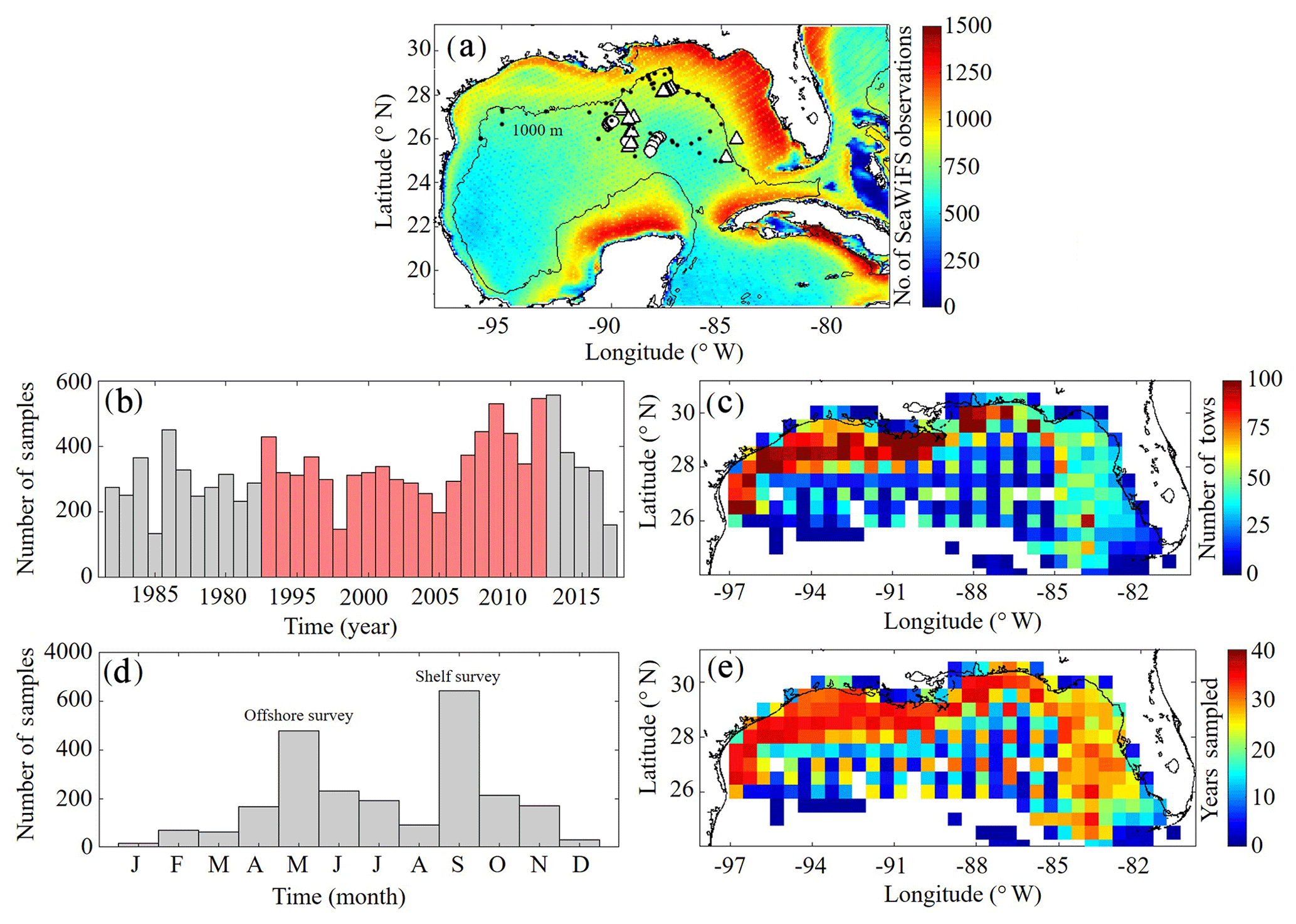
Figure 1(a–e) Spatial and temporal coverage of observational datasets used for model validation. Total number of nonzero values available in daily SeaWiFS images from September 1997 to 10 December 2010 along with nitrate profiles from the World Ocean Database (black dots) and the location of in situ measurements collected during May 2017 (circles) and May 2018 (triangles) process study cruises (a). Total annual sampling of the SEAMAP surveys from 1983 to 2017 with samples overlapping with the PBM simulation period denoted in red (b). SEAMAP samples organized by month (d). Total sample density within each box (c) along with the number of years with at least one sample (e). The 1000 m isobaths and coastline are denoted by black continuous lines.
2.3.2 Mesozooplankton biomass observations
To evaluate model mesozooplankton biomass estimates, we used plankton tows collected during Southeast Area Monitoring and Assessment Program (SEAMAP) surveys in the northern and central GoM. In total, 11 781 plankton tows were collected from 1983 to 2017, with two main annual surveys in the spring (offshore) and fall (shelf) (Fig. 1). On average, SEAMAP collected approximately 300 samples per year with a specific sampling array offshore and more general sampling coverage on the shelf. In total, 6835 samples were used for direct point-to-point model–data comparisons. Samples were collected using standard gear consisting of a 61 cm diameter bongo frame fitted with two 333 µm mesh nets. The nets were fished in a double-oblique tow pattern from the surface down to 200 or 5 m off the bottom and back to the surface. Simultaneous samples were also collected using a 202 µm mesh net during 82 tows. Of these samples, roughly half were collected in the oligotrophic GoM. The average ratio between biomass measured in the 333 and 202 µm bongo tows (0.5093±0.12) was used to convert 333 µm samples so that direct comparisons could be made with model mesozooplankton (LZ+PZ) biomass fields. Zooplankton biomass was originally quantified as displacement volumes (DVs). Carbon mass (CM) equivalents were subsequently calculated as log10(CM) = (log10(DV) +1.434)/0.820 (Wiebe, 1988; Moriarty and O'Brien, 2013).
For comparison to in situ biomass measurements, size ranges were assumed for zooplankton state variables (see Sect. 2.3.4). In NEMURO-GoM, SZ represent heterotrophic protists (e.g., ciliates) and early stages of mesozooplankton, which are typically < 200 µm in the ocean. Hence, SZ are assumed to range in size from 2 to 200 µm. LZ are considered to represent small mesozooplankton ranging in size from 0.2 to 1.0 mm, while PZ represent large mesozooplankton ranging in size from 1.0 to 5.0 mm. For comparison to the SEAMAP climatology the model LZ and PZ fields were first converted to units of carbon assuming Redfield C:N ratio and summed over the entire simulation before being depth averaged to the bottom or 200 m. For point-to-point model–data comparisons, total mesozooplankton biomass fields were interpolated to SEAMAP sample locations/times and then depth averaged to the corresponding sample tow depth.
2.3.3 Observed vertical profiles of chlorophyll and nitrate
Depth profiles of Chl were also collected during SEAMAP surveys using a Sea-Bird WETStar fluorometer attached to a CTD. Calibration of the fluorimeter was infrequent, and thus profiles were used to determine the depth of the fluorescence maxima for comparisons to DCM depths in the model. In total, 2435 profiles were collected from 2003 to 2012, with 1052 profiles overlying bottom depths > 1000 m. Profiles were available for earlier SEAMAP surveys; however, no standard QA/QC protocol for fluorometer data was in place prior to 2003.
To evaluate DCM magnitudes in the model, we used 145 fluorescence profiles collected during May 2017 and 2018 process study cruises (see Sect. 2.3.4). The fluorometer was attached to a CTD and calibrated using 126 in situ Chl samples. Chl concentrations were determined from filtered samples collected at depths ranging from 5 to 115 m using high-performance liquid chromatography (HPLC). Since the cruise sampling does not overlap with our NEMURO-GoM simulation period, model–data comparisons were made for all 20 years of the model run using sample locations and time of the year. This was also done with other field measurements from the process cruises (see Sect. 2.3.4).
For model–data comparisons of nitrate, we utilized profiles from the World Ocean Database (WOD). In total, 96 profiles were available during our simulation period and located in the oligotrophic GoM (> 1000 m isobath). Profiles were collected during all months except March and December, with the majority of samples collected during May, July and August (Fig. 1a).
2.3.4 Biomass and rate measurements from process study cruises
Although in situ rate measurements are made much less frequently than biological standing stock measurements, they offer very powerful constraints for validating the internal dynamics of a biogeochemical model (Franks, 2009). Consequently, we made phytoplankton and zooplankton rate measurements on two cruises in the open-ocean GoM in May 2017 and 2018 and used these measurements to validate the model (Fig. 1a). On the process study cruises, we utilized a quasi-Lagrangian sampling scheme to investigate plankton dynamics in the oligotrophic GoM. Two drifting arrays (one sediment trap array and one in situ incubation array) were deployed to serve as a moving frame of reference during ∼4 d studies (cycles) characterizing the water parcel (Landry et al., 2009; Stukel et al., 2015). During these cycles, we measured daily profiles of Chl, photosynthetically active radiation, phytoplankton growth rates and productivity, protistan grazing rates, and size-fractionated mesozooplankton biomass and grazing rates.
Size-fractionated mesozooplankton biomass and grazing rates were determined from daily day–night paired oblique ring-net tows (1 m diameter, 202 µm mesh). In total, 40 oblique bongo net tows (16 in 2017 and 24 in 2018) sampled the oligotrophic GoM mesozooplankton community from near surface to a depth ranging from 100 to 135 m. Upon recovery, the sample was anesthetized using carbonated water, split using a Folsom splitter, filtered through a series of nested sieves (5, 2, 1, 0.5 and 0.2 mm), filtered onto preweighed 200 µm Nitex filters, rinsed with isotonic ammonium formate to remove sea salt and flash frozen in liquid nitrogen. In the lab, defrosted samples were weighed for total wet weight and subsampled in duplicate (wet weight removed) for gut fluorescence analyses. The remaining wet sample was dried and subsequently reweighed and combusted for CHN analyses to determine total dry weight and C and N biomasses. Gut fluorescence subsamples were homogenized using a sonicating tip, extracted in acetone, and measured for Chl and phaeopigments using the acidification method. The phaeopigment concentrations in the zooplankton guts were the basis for calculated grazing rates using gut turnover times based on temperature relationships for mixed zooplankton assemblages. For additional details, see Décima et al. (2011, 2016).
Protistan grazing rates were measured using the two-point, mini-dilution variant of the microzooplankton grazing dilution method (Landry et al., 1984, 2008; Landry and Hassett, 1982). Briefly, one 2.8 L polycarbonate bottle was gently filled with whole seawater taken from six depths (from the surface to the depth of the mixed layer). A second 2.8 L bottle was then filled with 33 % whole seawater and 67 % 0.2 µm filtered seawater. Both bottles were then placed in mesh bags and incubated in situ at natural depths for 24 h. These experiments were conducted on each day of the ∼4 d cycle. After 24 h, the bottles were retrieved and filtered onto glass fiber filters, and Chl concentrations were determined using the acidification method (Strickland and Parsons, 1972). Net growth rates (k=ln(Chlfinal/Chlinit)) in each bottle were determined relative to initial Chl samples. Phytoplankton specific mortality rates resulting from the grazing pressure of protists were calculated as m= (kd–k0)/(1–0.33), where kd is the growth rate in the dilute bottle and k0 is the growth rate in the control bottle. Phytoplankton specific growth rates were calculated as . For additional details, see Landry et al. (2016) and Selph et al. (2016). Phytoplankton net primary production was quantified at the same depths by uptake experiments. Triplicate 2.8 L polycarbonate bottles and a fourth “dark” bottle were spiked with and incubated in situ for 24 h at the same sampling depths as for the dilution experiments. Samples were then filtered and the 13C:12C ratios of particulate matter determined by isotope ratio mass spectrometry.
3.1 Surface chlorophyll model–data comparisons
Model surface Chl estimates were found to agree closely with satellite observations reproducing patterns in both the oligotrophic and shelf region (Fig. 2). Spatial covariance between SeaWiFS climatology and model surface Chl climatology (calculated with daily cloud cover mask applied) is statistically significant (p < 0.01) with a correlation (ρ) of 0.72. When model estimates are compared to all 22 244 513 SeaWiFS measurements at corresponding times and locations (i.e., daily grid cell pairs), we find a ρ value of 0.50 (p < 0.01). To facilitate more detailed model–data comparisons, the GoM domain was divided into an oligotrophic region (> 1000 m bottom depth) and a shelf region (< 1000 m bottom depth). In the oligotrophic region, the correlation between model–data daily grid cell pairs is significant but weak (ρ=0.17, p < 0.01) as a result of relatively low large-scale spatial variability and hence dominance at the mesoscale. However, bias is quite low (−0.014 mg Chl m−3), equivalent to 10 % of the observed mean. In the shelf region, the correlation is higher (ρ=0.47, p < 0.01) yet the bias is greater (+0.90 mg Chl m−3), equivalent to 92 % of the mean. Previous GoM studies have determined ρ values for monthly averages, which we calculate here for comparison. Based on 30 d averages, the ρ values are 0.70 (p < 0.01) for the oligotrophic region and 0.26 (p < 0.01) for the shelf region.
In addition to resolving the dominant spatiotemporal variability, the model also captures the amplitude of the seasonal surface Chl signal reasonably well. In the oligotrophic region, the model accurately estimates the observed annual surface Chl minimum (model: 0.065±0.005 mg Chl m−3 vs. SeaWiFS: 0.065±0.007 mg Chl m−3) while slightly underestimating the observed annual maximum (model: 0.47±0.15 mg Chl m−3 vs. SeaWiFS: 0.75±0.55 mg Chl m−3). When model estimates for the entire oligotrophic region are taken into account (i.e., not restricted to satellite measurement locations and times), the annual minimum develops in early September, and the maximum develops in late January (Table 1). In the shelf region, greater model–data mismatch exists for surface Chl, with the model overestimating the observed annual minimum by 15 % (model: 0.23±0.09 mg Chl m−3 vs. SeaWiFS: 0.20±0.07 mg Chl m−3) and the observed annual maximum by 102 % (model: 8.09±1.31 mg Chl m−3 vs. SeaWiFS: 4.01±1.23 mg Chl m−3). Here, we find the annual surface Chl seasonal cycle almost completely out of phase with the oligotrophic region, with the annual minimum developing in early February and the annual maximum developing at the end of July (Table 1).
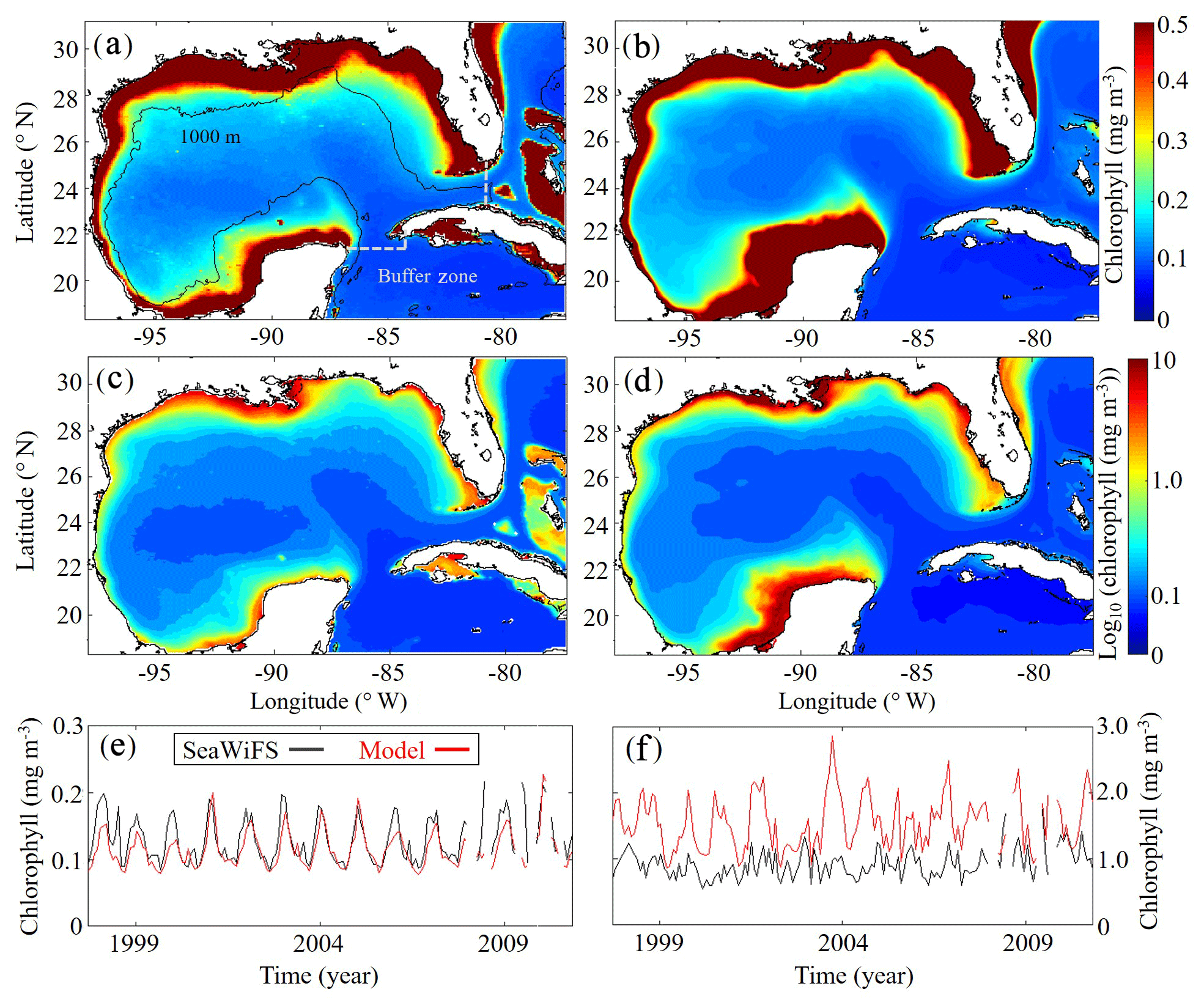
Figure 2(a–f) Comparison of surface chlorophyll (mg m−3) between SeaWiFS observations (a, c) and model (b, d) from 4 September 1997 to 10 December 2010. Surface chlorophyll climatology computed from daily SeaWiFS images (a) and the corresponding log10 field (c). Surface chlorophyll climatology computed from daily averages over the entire model simulation (1993–2012) (b) and the corresponding log10 field (d). Time series of simulated 30 d average surface chlorophyll based on SeaWiFS observations (black) and model (red) for the oligotrophic region (grid cells with bottom depths ≥1000 m) (e) and shelf region (grid cells with bottom depths < 1000 m) (f).
3.2 Regional mesozooplankton biomass model–data comparisons
Model mesozooplankton biomass (i.e., LZ + PZ) fields also agree closely with observations in both the oligotrophic and shelf region (Fig. 3). Spatial covariance between SEAMAP climatology and model is statistically significant (p < 0.01), with a ρ value of 0.90. When model estimates are compared to SEAMAP tows at corresponding sample times and locations for the 6835 measurements in the simulation period, the ρ value is 0.55 (p < 0.01). In the oligotrophic region, the model slightly overestimates mesozooplankton biomass (model: 4.09±1.82 mg C m−3 vs. SEAMAP: 3.52±3.44 mg C m−3), with a ρ value of 0.23 (p < 0.01) and a bias of 0.57 mg C m−3, equivalent to 16 % of the observed mean. Conversely, in the shelf region, the model underestimates mesozooplankton biomass (model: 17.40±13.58 mg C m−3 vs. SEAMAP: 20.91±24.62 mg C m−3), with a ρ value of 0.49 (p < 0.01) and a bias of −3.5 mg C m−3, equivalent to 17 % of the observed mean. Model estimates and SEAMAP measurements also compare well with total mesozooplankton biomass measurements (0.2–5 mm) collected in the oligotrophic region during the process study cruises (model: 5.55±2.87 mg C m−3 vs. cruise: 4.33±2.28 mg C m−3).
Although seasonal cycles in the oligotrophic and shelf regions could not be derived from the SEAMAP dataset given the significant differences in sampling locations over the course of a year, we investigated model–data mismatches for each month. The model closely matches or slightly underestimates mesozooplankton biomass for most of the year, with the exception of January, May and August (Fig. 3a). The largest model–data mismatch occurs during March, June, July and December, when the model underestimates mesozooplankton biomass by approximately 35 %. Unlike surface Chl, the total mesozooplankton biomass (i.e., depth-integrated) seasonality is similar in both regions of the GoM. In the oligotrophic region, the annual biomass minimum (maximum) occurs at the beginning of January (middle of May), while in the shelf region, the annual minimum (maximum) occurs in late December (end of May) (Table 1).
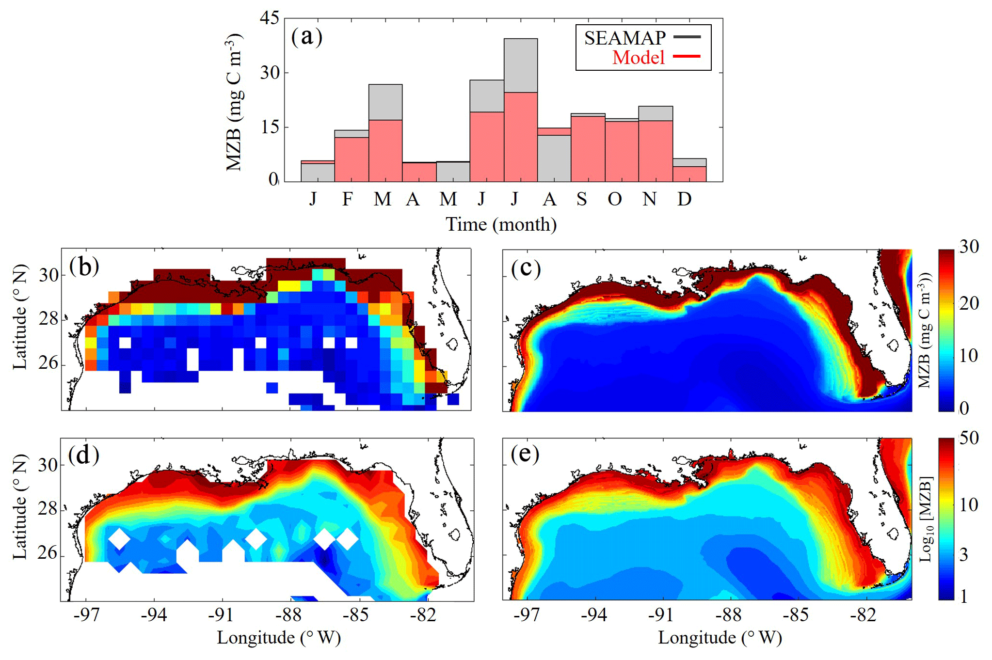
Figure 3(a–e) Comparison of climatological depth-averaged (0–200 m) mesozooplankton biomass (MZB, mg C m−3) between SEAMAP observations (b, d) and model (c, e). Monthly average MZB in SEAMAP observations (black) and model (red) (a) (monthly variability is not representative of MZB seasonality because sampling locations change between months). MZB climatology computed from SEAMAP plankton tows (b) and the corresponding log10 field (d). MZB climatology computed from daily averages over the entire model simulation (1993–2012) (c) and the corresponding log10 field (e).
3.3 Chlorophyll and nitrate profile model–data comparisons
To validate the vertical structure of the simulated ecosystem, we utilized observed profiles of fluorescence, Chl and nitrate. When simulated DCM depths were compared to all 2435 SEAMAP fluorescence profiles, we found a statistically significant correlation (ρ=0.59, p < 0.01) with the observed maximum fluorescence depth. The maximum fluorescence depth ranged from the surface to 143 m, while model values show a similar variability ranging from the surface to 163 m (Fig. 4a). In the oligotrophic region, the model overestimates the DCM depth (model: 95±20 m vs. SEAMAP: 80±25 m) and has a ρ value of 0.38 (p < 0.01) with a bias of 15 m, equivalent to 19 % of the observed mean. In the shelf region, the model also overestimates DCM depth (model: 63±26 m vs. SEAMAP: 53±23 m) and has a ρ value of 0.49 (p < 0.01) with a bias of 10 m, equivalent to 19 % of the observed mean.
In contrast, the model slightly underestimated the DCM depth when compared to calibrated fluorescence profiles collected during the process cruises (model: 100±18 m vs. observed: 107±21 m) (Fig. 4b). In terms of magnitude, the model overestimates DCM Chl (model: 0.74±0.35 mg Chl m−3 vs. observed: 0.38±0.13 mg Chl m−3), although most of the observations fall within 1 standard deviation of the model average. Despite this model–data mismatch, simulated nitrate profiles closely match profiles from the World Ocean Database (WOD). In both the model and observations, the mean nitracline occurred at approximately 75 m (Fig. 4c). On average, model nitrate tended to be lower at the surface and higher at depth relative to observations. Above the nitracline, model nitrate was 0.071±0.39 mmol N m−3 while observed nitrate was 0.55±1.29 mmol N m−3. Below 200 m, model and data show better agreement, with deep nitrate in the model of 24.92±3.28 compared to 23.55±5.21 mmol N m−3 in WOD profiles.
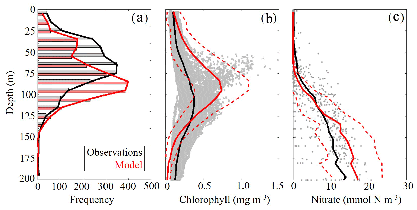
Figure 4(a–c) Model–data comparisons in the vertical distribution of chlorophyll (a, b) and nitrate (c). Comparison between maximum fluorescence depths observed in SEAMAP profiles and simulated maximum chlorophyll depths (m) (a). Comparison between in situ chlorophyll samples collected during May 2017 and 2018 process study cruises and simulated chlorophyll concentrations (mg m−3) (b). Gray dots represent cruise sample values and the red dashed line denotes 1 standard deviation away from the model average. Comparison between nitrate profiles obtained from the World Ocean Database (WOD) and simulated nitrate (mmol N m−3) (c). Gray dots represent WOD sample values and the red dashed line denotes 1 standard deviation away from the model average.
DCM depth was evaluated using uncalibrated fluorescence profiles obtained during SEAMAP cruises. Chlorophyll profiles were collected during the May 2017 and 2018 Lagrangian process cruises. For comparisons, the model and data were sampled at corresponding locations and time of the year for all simulated years. Nitrate values from the World Ocean Database that overlapped with the simulation period and were located in the oligotrophic GoM (> 1000 m) were used for model–data comparisons.
3.4 Size fractionated mesozooplankton biomass and grazing model–data comparisons
To further constrain the phytoplankton and zooplankton community simulated by NEMURO-GoM, we utilized in situ measurements collected during the process study cruises. First, we compared the relative proportions of LZ and PZ biomass to four discrete size classes measured at sea (Fig. 5a, c). In both the model and observations, we find nearly identical size distributions assuming that LZ approximates the smallest two size classes of mesozooplankton sampled (small mesozooplankton, 0.2–1.0 mm) and PZ approximates the largest two size classes (large mesozooplankton, 1.0–5.0 mm). In the field data, small mesozooplankton biomass varied from 33 % to 46 % (median =40 %, at 95 % C.I.), while model estimates of LZ biomass vary from 31 % to 46 % (median =40 %). Large mesozooplankton biomass in the field data varied from 54 % to 67 % (median =60 %), while model estimates of PZ biomass vary from 54 % to 69 % (median =60 %).
Mesozooplankton specific grazing rates measured during the process study cruises were also used to validate the simulated mesozooplankton community. Field measurements showed that specific grazing rates (µg Chl mg C−1 d−1) decreased consistently with increasing mesozooplankton size-class (Fig. 5b). For model–data comparisons, we computed grazing on LP by LZ and PZ at each depth. Grazing terms were converted into units of Chl using the model-estimated C:Chl ratio for LP before being depth-integrated to the corresponding net tow depth and normalized to simulated depth-integrated LZ and PZ biomasses. We find that model mesozooplankton grazing estimates capture the general trend of decreased specific grazing rates with increasing mesozooplankton size (Fig. 5d). However, the model overestimates grazing by small mesozooplankton while underestimating grazing by large mesozooplankton. In the field data, small mesozooplankton grazing ranges from 1.34 to 2.51 µg Chl mg C−1 d−1 (median =1.85) while model estimates of LZ grazing rates vary from 3.64 to 8.14 µg Chl mg C−1 d−1 (median =6.01). Field measurements of large mesozooplankton grazing range from 0.76 to 1.44 µg Chl mg C−1 d−1 (median = 0.94), while model estimates of PZ grazing vary from 0.44 to 0.70 µg Chl mg C−1 d−1 (median =0.58). In terms of total grazing, the model average is also considerably higher (2.99±2.20 µg Chl mg C−1 d−1) relative to field measurements (1.38±0.59 µg Chl mg C−1 d−1) (see Discussion).
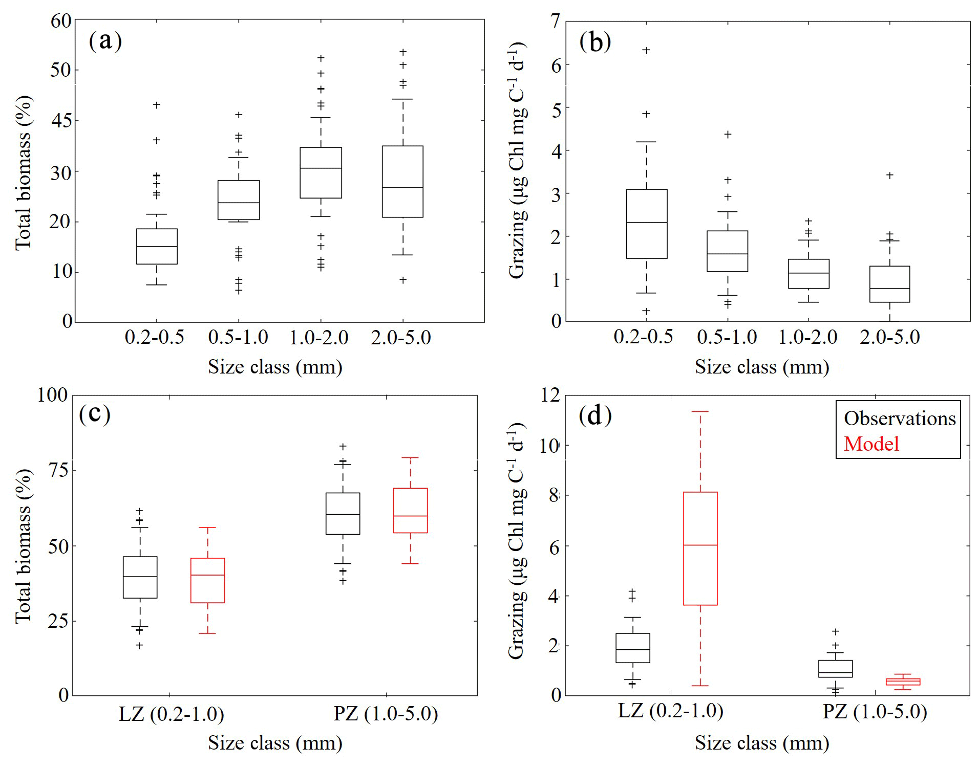
Figure 5(a–d) Mesozooplankton size-fractioned biomass (a, c) and grazing rates (b, d) in field measurements (black) and model estimates (red). Mesozooplankton size-fractioned biomass measured during May 2017 and May 2018 process study cruises (a) along with corresponding measured grazing rates (b). Comparisons of model-estimated mesozooplankton biomass to aggregated (size class 1–2 and 3–4) field measurements (c). Comparisons of model-estimated specific mesozooplankton grazing rates to aggregated (size class 1–2 and 3–4) field measurements (d). Whiskers extend to 95 % confidence interval. Outliers for model estimates are not shown.
3.5 Phytoplankton growth and microzooplankton grazing model–data comparisons
Measurements of specific phytoplankton growth rates, phytoplankton mortality due to microzooplankton grazing and net primary production (NPP) were used to evaluate protistan dynamics in the model. We find the model underestimates phytoplankton growth and microzooplankton grazing while overestimating NPP (Fig. 6a, b). Phytoplankton specific growth rates from dilution experiments range from 0.50 to 0.66 d−1 (median =0.55 d−1), while model estimates of phytoplankton (SP+LP) specific growth rates vary from 0.13 to 0.27 d−1 (median =0.21 d−1). In terms of microzooplankton grazing rates, field data range from 0.19 to 0.55 d−1 (median =0.39 d−1), while model estimates of SZ vary from 0.10 to 0.21 d−1 (median =0.16 d−1). NPP estimates show better agreement with observations, with rates from 276 to 360 mg C m−2 d−1 (median =321 mg C m−2 d−1) in field data, while model estimates vary from 190 to 741 mg C m−2 d−1 (median =431 mg C m−2 d−1).
Although the model underestimates phytoplankton growth and microzooplankton grazing rates, the relative proportion of NPP consumed by protists in the model (67 %–85 %; median =76 %) compares reasonably well to field measurements (55 %–92 %; median =72 %) (Fig. 6c). Notably, the model average proportion of phytoplankton production consumed by protists closely matches the mean for all tropical waters reported by Calbet and Landry (2004). When phytoplankton mortality due to mesozooplankton grazing was evaluated in the model at cruise sample locations, we found mesozooplankton grazing accounts for 13±8 %, which also closely agrees with the global average (Calbet et al., 2001).
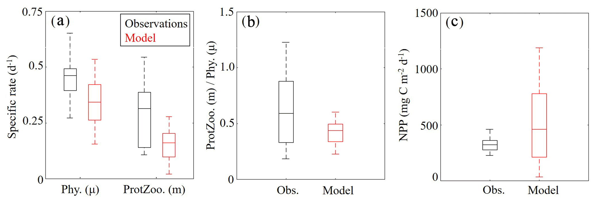
Figure 6(a–c) Specific phytoplankton growth (μ, d−1) and microzooplankton grazing (m, d−1) between model (red) and field data (black) (a). The fraction of phytoplankton growth that is grazed by protists in the model and field data (b). Depth-integrated net primary production (mg C m−2 d−1) (c). Whiskers extend to the 95 % confidence intervals. Outliers for model estimates are not shown.
3.6 Simulated mesozooplankton diet
After model tuning and validation, we utilized NEMURO-GoM to investigate spatiotemporal variability in diet and secondary production of the GoM mesozooplankton community. First, we examined the trophic level of LZ and PZ in the model, which provides a measure of their cumulative diet. Trophic level is calculated by computing the dietary contributions of each prey in LZ (i.e., LP and SZ) and PZ diets (i.e., LP, SZ and LZ), assuming that the trophic level of LP equals 1 and that of SZ equals 2. In the oligotrophic region, both LP and SZ contribute approximately 50 % to LZ diet, as indicated by a mean trophic level near 2.5 (2.54±0.02) for LZ (Fig. 7a). In the same region, PZ have a trophic level of 2.78±0.04, indicating a higher contribution of zooplankton to their diet (i.e., SZ and/or LZ) (Fig. 7b). In the shelf region, LZ are more herbivorous, as indicated by a decrease in trophic level to 2.31±0.01, while PZ are more carnivorous, as indicated by an increase in trophic level to 2.90±0.04.
Despite little evidence for LZ diets dominated by zooplankton in the annual average (in contrast to PZ, which often have a trophic level ∼3), we commonly find regions in instantaneous fields during both winter and summer conditions where SZ are the dominant prey source for LZ (Fig. 7c, e). These regions, typically in the Loop Current or Loop Current eddies (LCEs), highlight the episodic importance of heterotrophic protists as prey sources for small mesozooplankton in the GoM. High proportions of SZ in LZ diets can be attributed to the competitive advantage of SP over LP in extremely low nutrient environments such as in the Loop Current, resulting in high abundances of SP and their predators (SZ) relative to LP. Instantaneous fields also reveal that phytoplankton can be important prey for PZ as well, particularly during summer, as indicated by trophic levels of around 2.5 in the western GoM (Fig. 7f). In addition to strong variability in trophic positions, there are also regions in the oligotrophic GoM, most clearly in the centers of LCEs during summer, where the model predicts no feeding by mesozooplankton (Fig. 8e). The convergent anticyclonic circulation of LCEs is typically associated with low phytoplankton biomass, which at times may fall near or below feeding thresholds in the NEMURO grazing formulation. This formulation is intended to simulate suppression of feeding activity for zooplankton at mean prey densities that cannot support the energy expended while searching for prey.
To investigate which prey contributes most to LZ and PZ diets, we computed each prey source term for both LZ and PZ at each grid cell (Fig. 8). As one would expect, the dominant prey for LZ and PZ align closely with spatial variability in their respective trophic positions. For LZ diet, herbivory dominates throughout the GoM, except for the Loop Current (Fig. 8a). LP contribution to LZ diet is highest on the shelf, where LP biomass is also high due to the competitive advantage of LP over SP in high-nutrient conditions. In contrast, PZ diet varies with the relative availability of SZ and LZ prey. In the oligotrophic region, PZ feed mainly on SZ (heterotrophic protists) because LZ biomass is relatively low. On the shelf, they consume primarily LZ (Fig. 8d). Despite the significant change in diet between the shelf and oligotrophic regions, PZ trophic positions remain fairly consistent (Fig. 7d). This is due to the fact that SZ in the oligotrophic region and LZ in the shelf region both feed predominantly on phytoplankton and hence occupy similar trophic levels. In the instantaneous fields for winter (Fig. 8b, e) and summer (Fig. 8c, f), the dominant prey for both LZ and PZ show substantial mesoscale variability, indicating that oceanographic features such as fronts and eddies influence not only biomass but also zooplankton ecological roles (see Discussion).
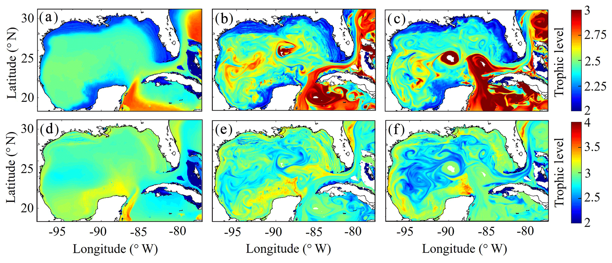
Figure 7(a–f) Trophic levels of simulated large zooplankton (LZ, a, b, c) and predatory zooplankton (PZ, d, e, f). Annual-averaged trophic positions of LZ (a) and PZ (d). Instantaneous model field of trophic positions during winter conditions for LZ (b) and PZ (e) on 4 February 2012. Instantaneous model field of trophic positions during summer conditions for LZ (c) and PZ (f) on 2 August 2011.
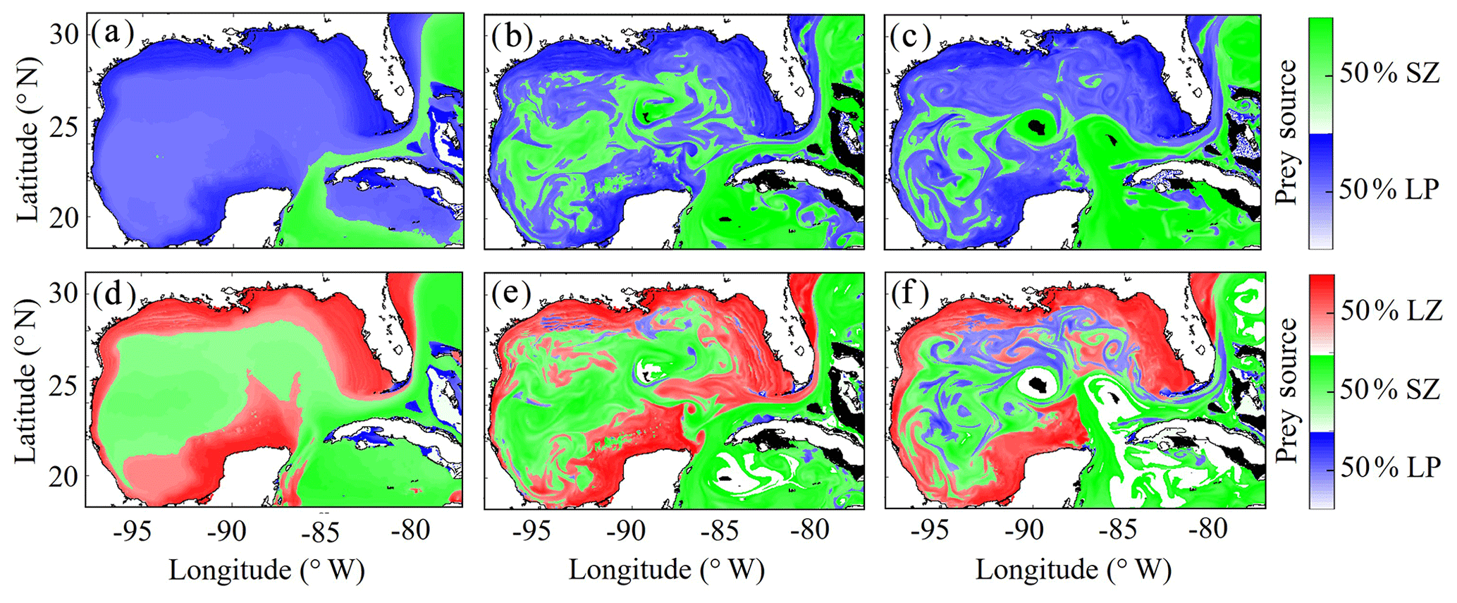
Figure 8(a–f) Dominant prey source for simulated large zooplankton (LZ, a, b, c) and predatory zooplankton (PZ, d, e, f). Annual-averaged diet contributions for LZ (a) and PZ (d). Instantaneous model field of zooplankton diet during winter conditions for LZ (b) and PZ (e) on 4 February 2012. Instantaneous model field of zooplankton diet during summer conditions for LZ (c) and PZ (f) on 2 August 2011.
3.7 Simulated mesozooplankton secondary production
To our knowledge, regional secondary production for the GoM has not been quantified previously. Based on our model, secondary production due to mesozooplankton averages kg C yr−1 and ranges from a minimum of 51×109 kg C (in 1999) to a maximum of 82×109 kg C (in 2011). In the oligotrophic region, LZ secondary production averages 35±5 mg C m−2 d−1 while PZ secondary production is 11±2 mg C m−2 d−1 (Fig. 9). The annual secondary production minimum develops at the end of December, while the annual maximum occurs at the beginning of June (Table 1). In this region, mesozooplankton secondary production is kg C yr−1, equivalent to 6 % of NPP. On the shelf, secondary production is about 4-fold higher, with LZ production of 146±17 mg C m−2 d−1 and PZ production of 42±5 mg C m−2 d−1. Here, the annual minimum also occurs at the end of December while the maximum occurs later at the end of July (Table 1). On the shelf, secondary production constitutes a higher proportion of NPP (13 %) and averages kg C yr−1.
In addition to differences in total secondary production, significant differences were found in the mesozooplankton community response to changes in total phytoplankton biomass on the shelf and in the oligotrophic region. On the shelf, the average ratio between LZ and PZ secondary production is 3.51 and remains almost constant with increasing phytoplankton biomass (ρ=0.13, p < 0.01). Although we find a similar average value in the oligotrophic region (3.14), ratios are more variable and strongly dependent on phytoplankton biomass (ρ=0.52, p < 0.01). Ratios of LZ to PZ secondary production reached values of ∼2.5 in the lowest phytoplankton biomass regions of the open-ocean GoM and increased to ∼4.0 during times and places where local phytoplankton biomass was high. These differences likely stem from the longer turnover times of PZ, which make them less sensitive to variability in bottom-up drivers and allow them to have a proportionally greater role in oligotrophic settings.
As witnessed in the instantaneous fields of diet and secondary production, mesoscale eddies are common features in the GoM and hence important to quantify for regional zooplankton dynamics. To investigate secondary production inside cyclonic and anticyclonic eddies, we implement the TOEddies eddy detection algorithm (Laxenaire et al., 2018), which uses surface velocities along closed contours of sea surface height (SSH) for detection of mesoscale eddies (Chaigneau et al., 2011; Laxenaire et al., 2019; Pegliasco et al., 2015). Grid cells located inside each eddy are defined within the SSH contour associated with the maximum mean surface velocity (interior grid cells). Grid cells located between the outermost closed contour and within 1.5 radius of the eddy center and not within another eddy were used to define background conditions outside of eddies (exterior grid cells). Only eddies with areas larger than an equivalent circular diameter of 100 km and not within the Loop Current were considered in the analysis. On average, 3.78 cyclonic and 3.33 anticyclonic eddies were identified in each daily velocity field.
In the model, cyclonic eddies were associated with 10 % higher secondary production relative to exterior grid cells, and the ratio of secondary production in interior cells to exterior cells ranged from 0.4 to 3.37 (95 % CI). In contrast, secondary production was substantially lower inside anticyclonic eddies, accounting for only 46 % of the average secondary production in exterior cells (0.03–1.87, 95 % CI). In addition to their convergent nature that dampens nutrient input, lower rates of secondary production in anticyclonic eddies can likely be attributed to the presence of highly oligotrophic Loop Current water trapped within large anticyclonic LCEs.
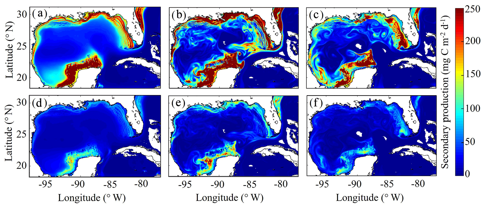
Figure 9(a–f) Vertically integrated secondary production (mg C m−2 d−1) of simulated large zooplankton (LZ, a, b, c) and predatory zooplankton (PZ, d, e, f). Annual-averaged secondary production for LZ (a) and PZ (d). Instantaneous model field of secondary production during winter conditions for LZ (b) and PZ (e) on 4 February 2012. Instantaneous model field of secondary production during summer conditions for LZ (c) and PZ (f) on 2 August 2011.
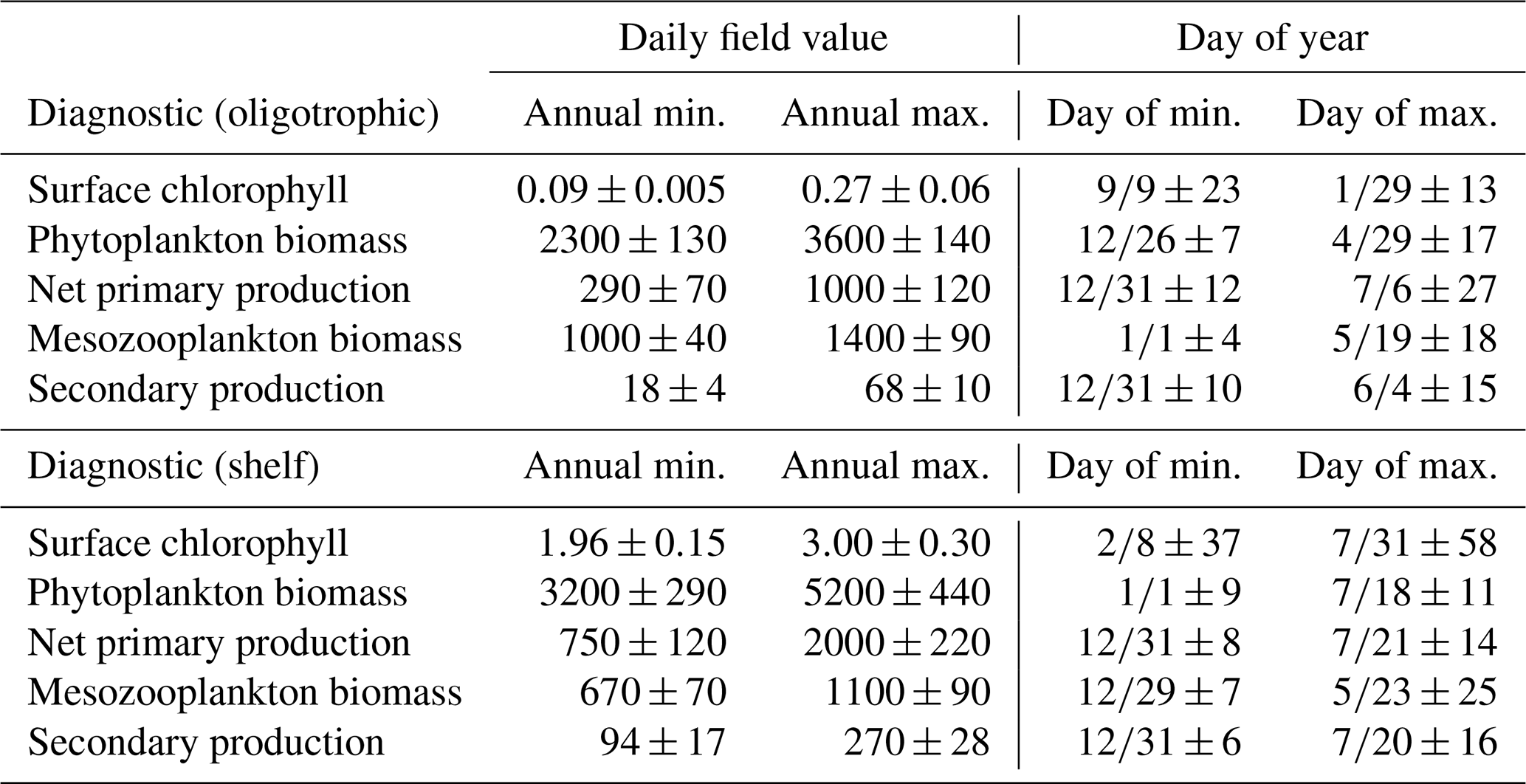
Table 1Average seasonal minimum and maximum values in the model (1993–2012) and the day of year in which they occur for surface chlorophyll (mg m−3), depth-integrated estimates of phytoplankton biomass (mg C m−2), net primary production (mg C m−2 d−1), mesozooplankton biomass (mg C m−2), and mesozooplankton secondary production (mg C m−2 d−1) calculated by spatially averaging daily fields over the oligotrophic region (grid cells with bottom depths > 1000 m) and shelf region (grid cells with bottom depths < 1000 m). Day of year values are in the format “month/day ± days”.
Many parameters in biogeochemical models are poorly constrained by observations and laboratory studies and/or highly variable in the environment. The numbers and uncertainties around these parameters allow PBMs with varying degrees of tuning to reproduce a single ecosystem attribute (e.g., surface Chl) even if multiple processes are inaccurately represented (Anderson, 2005; Franks, 2009). Once validated, one of the main values of coupling physical and biogeochemical models (i.e., PBMs) is their utility for making inferences about portions of the lower trophic level that are undersampled and/or difficult to measure in the field. If PBMs are to be utilized to explain variability rather than simply fit an observational dataset, multiple ecosystem attributes must be validated and the underlying model structure and assumptions critically evaluated. In the section below, we further justify changes to model structure by evaluating the underlying assumptions in default NEMURO, and we discuss model–data mismatch before drawing conclusions about the GoM zooplankton community and the implications of its dynamics for higher trophic levels.
4.1 Justification for NEMURO modifications
The phytoplankton community in the North Pacific (NP) domain where NEMURO was originally designed is largely composed of nanoplankton (original SP) and microplankton (original LP). By default, SP is assumed to represent coccolithophores and autotrophic nanoflagellates, which can be important prey of copepods and other mesozooplankton in temperate and subpolar regions (Kishi et al., 2007). However, in tropical regions such as the GoM, smaller picophytoplankton taxa typically dominate, particularly in highly oligotrophic regions. Common picophytoplankton of the GoM include cyanobacteria and picoeukaryotes, which are too small for most mesozooplankton to feed on. Hence, the SP-to-LZ grazing pathway was removed in our model. We found that removal of this grazing pathway allowed the model to simulate a more realistic phytoplankton community on the shelf region. Despite intuition, SP largely dominated the shelf region in the model when LZ were allowed to graze on SP. After closer inspection, we found that grazing of SP sustained LZ biomass on the shelf to levels where top-down pressure constrained LP standing stocks. This prevented large blooms of LP, leading to a competitive advantage for SP even in highly eutrophic conditions (the Mississippi River delta), which was observed for a wide range of LP maximum growth rates, LP half-saturation constants, and LZ and PZ grazing rates. Thus, removal of the SP to LZ grazing pathway added ecological realism and improved the model solution.
During the model tuning process (outlined in the Supplement), we also found that, despite a wide range of tested parameter sets, the model was unable to simulate mesozooplankton biomass low enough to match SEAMAP observations in the oligotrophic region. Even with unrealistically low phytoplankton biomass, equivalent to approximately 50 % of surface Chl observed in SeaWiFS images, the model overestimated mesozooplankton biomass. To achieve realistic levels of mesozooplankton biomass in the oligotrophic region, default LZ and PZ mortality parameter values needed to be increased by an order of magnitude. However, this produced unrealistically high loss rates on the shelf region, leading to mesozooplankton biomass estimates that were substantially lower than SEAMAP shelf observations. Implementation of linear mortality on all biological state variables (except PZ) resolved this issue by providing the model with a greater dynamic range. In NEMURO, and other biogeochemical models, quadratic mortality is often used to increase model stability and/or is mechanistically justified as representing the impact of unmodeled predators that covary in abundance with prey (Gentleman and Neuheimer, 2008; Steele and Henderson, 1992). However, grazing losses of all state variables (except PZ) are already explicitly modeled in NEMURO by default. Hence, removal of quadratic mortality also added ecological realism and improved the model solution. Quadratic mortality was retained for PZ to account for the implicit predation pressure of unmodeled predators (e.g., planktivorous fish).
4.2 Model–data mismatch
4.2.1 Surface chlorophyll discrepancies
Within our model–data comparisons of surface Chl we find that NEMURO-GoM reproduces important patterns in both the oligotrophic and shelf region, the latter of which, apart from the northern shelf, has not been well resolved by previous PBMs (e.g., Gomez et al., 2018; Xue et al., 2013). The absence of a shelf Chl signature may, in some cases, be overly attributed to bias in satellite measurement due to high concentrations of colored dissolved organic matter (CDOM). While a clear shelf signature is well resolved in NEMURO-GoM, the model–data mismatch is greater on the shelf compared to oligotrophic regions. This is an expected result considering that the model incorporates climatological river forcing while actual variability is much more complex. Furthermore, the absence of CDOM in the model likely contributes to the overestimation of phytoplankton biomass on the shelf.
In future studies, the inclusion of daily nutrient data like that produced for the Mississippi River by USGS starting in 2011 is needed for PBMs to better resolve variability on the shelf. Including benthic processes, such as denitrification (Fennel et al., 2006), may also reduce model–data mismatch in shelf regions. Implementing more realistic light attenuation (e.g., wavelength-specific light attenuation or inclusion of CDOM) could further improve estimates of phytoplankton biomass on the shelf as primary production can be sensitive to different light attenuation formulations (Anderson et al., 2015). In our model, it was difficult to simulate deep DCMs in the oligotrophic GoM while also simulating DCMs on the shelf that were shallow enough to maintain high nitrate. This may reflect the need for more realistic light attenuation in the model.
Quantifying uncertainty in C:Chl ratios is also an important task moving forward as future PBMs will likely continue to depend heavily on satellite Chl for the bulk of model validation. To correctly parameterize C:Chl ratios, more in situ samples are needed that resolve changes in phytoplankton light-harvesting pigments along gradients from coastal to oligotrophic regions and from the surface to the DCM. Without these observations, it is difficult to gauge mismatches between model and satellite ocean color products (e.g., discrepancies on the Campeche Bank in our model) or in situ profiles of Chl. In addition to validation, these measurements are needed to avoid erroneous model tuning. For instance, a model that exhibits significant mismatch with respect to surface Chl may in fact accurately estimate carbon-based phytoplankton biomass while using unrealistic C:Chl ratios. One could arrive at incorrect conclusions about regional ecosystem dynamics as a result of modifying model parameters or structure in an effort to better fit Chl observations. Given the importance of C:Chl ratios in PBMs, future studies should quantify uncertainty in modeled Chl through sensitivity experiments focused on C:Chl model parameters and formulation, with explicit comparison to direct field measurements of phytoplankton C:Chl.
In our model, the most noticeable surface Chl model–data mismatch occurs on the southern GoM shelf (Campeche Bank), where the model consistently overestimates surface Chl. This bias was also notable in the GoM PBM implemented by Damien et al. (2018), particularly in winter. We believe this discrepancy is driven by a combination of errors involving overestimation of shelf mixing by the hydrodynamic model, entrainment of high-Chl water (given the overestimated DCM magnitude in the model) or errors in the open boundary conditions which result in an overestimation of upwelled nutrients/biomass near the Yucatán Peninsula that are transported westward by shelf currents. We found that the Campeche Bank model–data mismatch was reduced when open boundary conditions included nitracline depths of greater than 100 m. This may reflect realistic in situ conditions considering that Caribbean water entering the GoM is highly oligotrophic. During our process cruises, nitrate was often undetectable above 100 m in samples collected near the Loop Current (Angela Knapp, personal communication, 2018).
Although modifying the boundary conditions may be justified, deepening the nitracline at the boundaries made it increasingly difficult to sustain realistic surface phytoplankton biomass in the oligotrophic GoM. This may point to the importance of nitrogen-fixing cyanobacteria, which provide an alternative source of new nitrogen (other than upwelling and mixing) that could be supporting phytoplankton at the surface given the strong stratification and deep nitraclines in the GoM. In the process of model tuning, we noticed that increasing the DON pool by increasing the PON to DON decomposition rate was necessary to maintain both relatively deep nitraclines and realistic surface Chl by providing a slow leeching of ammonium near the surface through bacterial communities. The need for this slow production of ammonium in surface layers may compensate for nitrogen fixation, which is not included in NEMURO (Holl et al., 2007; Mulholland et al., 2006). In future studies, including diazotrophs as a separate phytoplankton functional type would be essential for evaluating the importance of nitrogen fixation in the GoM.
Despite the model–data mismatch on the Campeche Bank, this discrepancy appears to have little impact on the rest of the GoM. However, the model overestimates surface Chl in the southwestern GoM, which can likely be attributed to entrainment of high-Chl water originating from the Campeche Bank. Locally, the ecological impact is likely more significant. Higher phytoplankton biomass would be expected to support higher mesozooplankton grazing rates and secondary production. Indeed, some of the highest model rates of secondary production occur on the Campeche Bank. Hence, the surface Chl model–data mismatch may lead to an overestimation of secondary production for this region.
4.2.2 Deep chlorophyll maximum discrepancies
Since most PBMs focus on validating against satellite-derived surface chlorophyll, the dynamics of the DCM is often insufficiently investigated. Consequently, many models predict DCM depths that are far too shallow. Identifying this issue in the literature proved to be difficult because most studies do not provide profiles of simulated Chl (an exception is the recent GoM PBM by Damien et al., 2018). We note that DCM depths in the DIAZO model (Stukel et al., 2014) were often quite shallow or completely nonexistent in the portion of the domain that included the oligotrophic GoM region. Underestimates of DCM depth in the unmodified COBALT biogeochemical model have also been identified (Moeller et al., 2019). In our investigation of the GoM PBM implemented by Gomez et al. (2018), we found that DCMs in the oligotrophic region were commonly shallow and weak. In the default NEMURO simulation, DCM depths in the oligotrophic region were typically at a depth of 25 m, which is much shallower than observed (SEAMAP: 80±25 m, Process cruises: 107±21 m). While this issue may seem insignificant, particularly if a study is focused on mixed-layer dynamics, accurate placement of the DCM can have profound impacts on PBM behaviors, because the DCM is typically colocated with the nitracline. Unrealistically shallow DCMs and nitraclines permit unrealistically high nitrate fluxes into the surface layer following mixing events; thus, validating the DCM in PBMs is critical.
For these reasons, we devoted substantial effort to tuning phytoplankton dynamics in the DCM. Modifications to α (the slope of the photosynthesis–irradiance curve) and attenuation coefficients allowed the model to estimate deeper more realistic DCM depths. Inclusion of a variable C:Chl module was also implemented to better resolve the DCM. However, an additional issue was present in the default NEMURO simulations, the NEMURO-GoM, and every simulation that we attempted. In all simulations that formed DCMs, the location of the DCM was always colocated with a maximum in phytoplankton specific growth rate, even though field measurements indicate that phytoplankton growth rates and NPP are either relatively constant with depth or decline in the DCM. This is not surprising, given the low photon flux at the base of the euphotic zone and the energetic demands required to upregulate cellular density of light-harvesting pigments. Additionally, our field measurements show that the DCM was not associated with a biomass maximum (biomass was fairly constant with depth), suggesting that DCM formation in the GoM is physiologically driven.
We believe this DCM dynamical issue was responsible, in part, for the underestimation of specific phytoplankton growth and microzooplankton grazing rates by the model despite estimating higher NPP (Fig. 4d). An underestimation of C:Chl ratios or overestimation of phytoplankton biomass may also contribute to the model–data mismatch at the DCM. The ecological impact of this mismatch is likely to be greatest in the model during the summer months when the mixed-layer depth is shallow and the DCM reaches its maximum depth. Elevated growth rates or biomass at the DCM during this period could significantly decrease nitrate flux into the mixed layer, causing the model to underestimate near-surface primary and secondary production.
Future PBM studies need to focus more effort on resolving ecological dynamics responsible for the formation of the DCM. Errors originating from the hydrodynamic model or use of temporally averaged velocity fields used in offline models may also contribute to model–data mismatch at the DCM. Vertical mixing is particularly important to PBMs but is often poorly validated in hydrodynamic models. Greater coordination between physical modelers and biologists to constrain vertical fluxes should be considered an important avenue for improving PBM simulations moving forward.
4.2.3 Mesozooplankton grazing discrepancies
Novel to this study, model estimates of mesozooplankton biomass are shown to agree closely with observations on the shelf and in the oligotrophic GoM. To our knowledge, this study includes the first quasi-regional zooplankton biomass model validation in a PBM. Our model also provides the first model–data comparisons of size-specific zooplankton biomass and grazing rates for the GoM. Such comparisons provide valuable insights into the potential biases of traditional functional-group biogeochemical models pertaining to zooplankton dynamics (Everett et al., 2017). While NEMURO-GoM shows broad agreement with zooplankton observations, some model–data mismatch occurs, particularly for mesozooplankton grazing rates.
We identify three factors that may explain the model–data mismatch for mesozooplankton grazing rates. The first and most obvious factor is the temporal sampling discrepancy as measurements were collected outside our model simulation period. Model–data mismatch may also arise from inaccuracies in the field measurements. During our process cruises, the zooplankton gut pigment measurements were based solely on phaeopigment content due to phytodetrital aggregates and Trichodesmium colonies found in our zooplankton net tows, which can lead to substantial contamination. Thus, true mesozooplankton grazing rates were likely underestimated because undegraded Chl can be abundant in the foreguts of mesozooplankton. Furthermore, the gut pigment approach assumes that any group of mesozooplankton has a constant gut throughput time (as a function of temperature), which is an oversimplification.
Uncertainties in model grazing formulations could also contribute to model–data mismatch (Gentleman et al., 2003a; Sailley et al., 2015). Future in situ grazing measurements are needed to enable an objective selection of grazing formulations and parameter values. In particular, field studies that shed light on prey selectivity would be useful for parameterizing PBMs with multiple mesozooplankton functional groups, such as NEMURO-GoM. Such studies are challenging, however, because the difficulty of making in situ grazing measurements on mesozooplankton, combined with the inherent uncertainty of these measurements, can make it challenging to differentiate between, for instance, Ivlev and Holling's disk grazing formulations (e.g., Fig. 4 in Morrow et al., 2018). Nevertheless, differences in parameterizing grazing can lead to substantially different model behavior (Anderson et al., 2010; Sailley et al., 2015; Wainwright et al., 2007). In NEMURO-GoM, secondary production and dietary preferences of the mesozooplankton community are both strongly influenced by model grazing formulation. While we carefully chose parameterizations that gave reasonable fits to extensive field datasets of zooplankton biomass and grazing rates, this does not preclude the possibility that other functional forms would have more accurately simulated zooplankton dynamics. Hence, future PBMs should investigate how different grazing formulations impact zooplankton dynamics in the region. We especially recommend collaborations between experimentalists (potentially using new techniques such as DNA metabarcoding of gut contents) and modelers to develop synthetic approaches with the potential to quantitatively assess the realism of different grazing formulations.
Clear model–data mismatch is also evident in the proportion of grazing mediated by PZ and LZ. This may be due to the fact that PZ is by default explicitly defined and parameterized as a higher-trophic-level mesozooplankton that can feed on LZ. In reality, while there is a correlation between size and trophic level in the ocean, many predatory zooplankton are < 1 mm, and many suspension-feeding zooplankton are > 1 mm; hence, the overlap of taxonomic groups with different functional roles and sizes makes it difficult to directly compare model categories to field data. For example, shelf suspension-feeding zooplankton are likely larger than their counterparts in the oligotrophic GoM although their functional role in the ecosystem does not change between environments.
The ecological impact of the model's potential overestimation of LZ grazing rates is most likely to manifest through an increase in the ratio of secondary production to mesozooplankton biomass. Since both LZ and PZ biomasses are accurately modeled by NEMURO-GoM, the overestimation of grazing rates suggests that LZ turnover times may be too high, thus leading to higher estimates of secondary production. However, this interpretation may oversimplify the complex interactions within pelagic protistan communities. In the oligotrophic region where our model overestimates LZ grazing rates, the model indicates that heterotrophic protists comprise approximately half of the LZ diet. Thus, overestimates of grazing on LP do not necessarily lead to overestimates in total consumption if < 1 mm zooplankton derive substantial nutrition from nonphototrophic sources in the field. Furthermore, the model's construction (i.e., LZ and PZ are functional groups, while the field data are size classes) suggests that part of the model–data mismatch in Fig. 5d may result from the presence of some suspension feeders (i.e., LZ) in the > 1 mm zooplankton size class and some carnivorous zooplankton (i.e., PZ) in the < 1 mm zooplankton size class. In this case, the model may simply attribute too high of a LP:SZ prey ratio to LZ. If this is the issue, the model's estimate of LZ secondary production may be accurate but its trophic level too low (or, conversely, the trophic level of PZ too high). Direct assessments of zooplankton trophic position (e.g., by compound-specific isotopic analysis of amino acids, Chikaraishi et al., 2009; Décima et al., 2017) may help resolve these issues.
4.3 Mesozooplankton dynamics in the open-ocean oligotrophic Gulf of Mexico
Despite its nutrient-poor conditions, the open-ocean GoM ecosystem is a key region for spawning and larval development of many commercially important fishes, including Atlantic bluefin tuna, yellowfin tuna, skipjack tuna, sailfish and mahi mahi (Cornic and Rooker, 2018; Kitchens and Rooker, 2014; Lindo-Atichati et al., 2012; Muhling et al., 2017; Rooker et al., 2012, 2013). Why so many species choose such oligotrophic waters as habitat for their larval stages is unknown but may be due to reduced predation risk (Bakun, 2013; Bakun and Broad, 2003). Regardless, rapid growth and survival through the larval period depend on mesozooplankton prey that are suitably abundant and appropriately sized for these larval fishes. These prey taxa may be especially sensitive to increased stratification and oligotrophication associated with climate change, making investigation of their dynamics and production an important topic of research.
Mesozooplankton biomass in the oligotrophic GoM was found to be strikingly low in both observations and model estimates, approximately an order of magnitude less than on the shelf. Model results clearly show that this low biomass condition arises from bottom-up resource limitation. Our results suggest that low phytoplankton biomass in oligotrophic regions, and particularly within Loop Current eddies, may even lead to localized and episodic regions where phytoplankton concentrations approach thresholds low enough that trigger collapse of mesozooplankton grazing. Prey-limiting conditions for mesozooplankton and their predators would be expected more frequently in the GoM during warmer ocean conditions. Higher sea surface temperatures and increased thermal stratification could suppress vertical mixing, resulting in lower phytoplankton biomass.
Despite extreme oligotrophy and dominance of picophytoplankton, our model shows that both PZ and LZ can be sustained at modest abundances in the oligotrophic GoM. Indeed, the substantial abundances of large (> 1 mm) mesozooplankton, equivalent to 60 % of total mesozooplankton in both observations and model results (Fig. 4a, c), are an important result that helps explain the success of larval fish in the region. Our results show that large mesozooplankton (PZ) occupy a trophic position of approximately 3.0 in the open-ocean GoM, which is marginally lower than on the shelf where they feed primarily on small mesozooplankton (LZ). The change in trophic position is associated with a switch from carnivory to feeding predominantly on heterotrophic protists in the oligotrophic region. This result highlights the importance of intermediate protistan trophic levels in sustaining mesozooplankton communities in oligotrophic regions. Indeed, both LZ and PZ ingest proportionally more SZ in the open ocean than on the shelf. Notably, these protistan trophic steps cannot be quantified by routine field techniques because they have no pigment signature to make them visible in gut pigment measurements and may not enrich in bulk 15N, leading to isotopic invisibility from a trophic perspective (Gutiérrez-Rodríguez et al., 2014). Despite their importance to phytoplankton grazing, they are sometimes missing from GoM ecosystem models (e.g., Fennel et al., 2011) and severely underrepresented or even absent in complex mass-balance constrained models (Arreguin-Sanchez et al., 2004; Geers et al., 2016). New insights may arise from focused investigations of phytoplankton–protist–crustacean linkages in oligotrophic regions in both model and experimental studies. This will likely require the use of next-generation technologies such as compound-specific isotopic analyses of specific amino acids that have been shown to enrich in protists (Décima et al., 2017) or DNA metabarcoding to assess zooplankton gut contents (Cleary et al., 2016).
Another robust finding from this study is the dynamic mesoscale variability in zooplankton abundance, diet and trophic position. These model results highlight the impact of Loop Current eddies and mesoscale fronts and other features in modifying the biogeochemistry and food web of the GoM. The existence of hot spots of productivity in the GoM has been noted in observational studies (Biggs and Ressler, 2001), and the importance of GoM mesoscale features to fish larvae has been hypothesized (Domingues et al., 2016; Lindo-Atichati et al., 2012; Rooker et al., 2012). Indeed, cyclonic eddies were found to have enhanced secondary production in our model, while secondary production was depressed within anticyclonic eddies. Our results further suggest that these mesoscale structures may not only modify zooplankton abundances, but also their trophic roles in the ecosystem, with implications for the transfer efficiencies of carbon and nitrogen in the pelagic food web.
In this study we developed a PBM for the GoM and after extensive validation used the model to investigate zooplankton community dynamics. The model was able to capture broad ecosystem attributes including phytoplankton and mesozooplankton abundances, depth of the DCM and nutricline, and growth and grazing patterns. Based on model estimates of trophic position and diet our results suggest that on the shelf small mesozooplankton are strongly herbivorous while large mesozooplankton are strongly carnivorous. However, distinct changes in diet were noted in the oligotrophic GoM, where both groups rely more on protistan prey. Changes in diet and secondary production highlighted in this study have the potential to impact food availability to higher trophic levels, such as pelagic larval fishes. In future work, we plan to couple NEMURO-GoM to an individual-based model to evaluate the extent to which mesozooplankton abundance limits larval fish feeding, growth and survival along transport pathways in the GoM. Insights from this ecosystem-based approach may help to better resolve stock-recruitment relationships that are needed for sustainable fisheries management and improved stock-assessment models.
The model code and model validation data used in this study can be downloaded from GitHub at https://github.com/tashrops/NEMURO-GoM (Shropshire, 2019a). An idealized one-dimensional version of NEMURO-GoM written in MATLAB is also provided. The three-dimensional NEMURO-GoM model outputs used in the study are available on the FSU-COAPS server in a Network Common Data Form (NetCDF format). Data are also publicly available through the Gulf of Mexico Research Initiative Information and Data Cooperative (GRIIDC) at https://data.gulfresearchinitiative.org (Shropshire, 2019b, https://doi.org/R6.X803.000:0018T).
The supplement related to this article is available online at: https://doi.org/10.5194/bg-17-3385-2020-supplement.
TAS conducted all numerical simulations and model analysis. EPC, SLM and AB provided expertise on the hydrodynamic modeling. MRS and VJC provided expertise on the biogeochemical model coding and tuning. RS, MRS, MRL and GZ processed and provided data that were central to NEMURO-GoM's validation. TAS wrote the manuscript with contributions from all authors.
The authors declare that they have no conflict of interest.
We thank the captains and crew of the NOAA ship Nancy Foster and many of our colleagues from NOAA SEFSC and the NASA-funded Predicting, Validating, and Understanding Zooplankton Distributions from Space in an Eddy Rich Ocean project. We also thank Oliver Jahn for providing valuable direction in configuring the offline MITgcm package as well as Mandy Karnauskas, Sang-Ki Lee and Fabian Gomez for their input during model development. We also thank Rémi Laxenaire for assistance with the TOEddies eddy detection algorithm.
This paper is a result of research supported by the Gulf of Mexico Research Initiative under the CSOMIO project, the NOAA RESTORE Science Program under federal funding opportunity NOAA-NOS-NCCOS-2017-2004875, the NOAA Center for Coastal and Marine Ecosystems (NOAA Office of Education, Educational Partnership Program, award NA16SEC48100009), the NOAA NMFS Fisheries and the Environment program, the Northern Gulf Institute (projects 18-NGI3-41 and 18-NGI3-52) under NOAA award NA16OAR4320199, and by NASA IDS grant no. 80NSSC17K0560.
This paper was edited by Katja Fennel and reviewed by three anonymous referees.
Anderson, T. R.: Plankton functional type modelling: Running before we can walk?, J. Plankton Res., 27, 1073–1081, https://doi.org/10.1093/plankt/fbi076, 2005.
Anderson, T. R., Gentleman, W. C., and Sinha, B.: Influence of grazing formulations on the emergent properties of a complex ecosystem model in a global ocean general circulation model, Prog. Oceanogr., 87, 201–213, https://doi.org/10.1016/j.pocean.2010.06.003, 2010.
Anderson, T. R., Gentleman, W. C., and Yool, A.: EMPOWER-1.0: an Efficient Model of Planktonic ecOsystems WrittEn in R, Geosci. Model Dev., 8, 2231–2262, https://doi.org/10.5194/gmd-8-2231-2015, 2015.
Arreguin-Sanchez, F., Zetina-Rejón, M., Manickchand-Heileman, S., Ramírez-Rodríguez, M., and Vidal, L.: Simulated response to harvesting strategies in an exploited ecosystem in the southwestern Gulf of Mexico, Ecol. Model., 172, 421–432, https://doi.org/10.1016/j.ecolmodel.2003.09.016, 2004.
Bakun, A.: Ocean eddies, predator pits and bluefin tuna: Implications of an inferred “low risk-limited payoff” reproductive scheme of a (former) archetypical top predator, Fish Fish., 14, 424–438, https://doi.org/10.1111/faf.12002, 2013.
Bakun, A. and Broad, K.: Environmental “loopholes” and fish population dynamics: Comparative pattern recognition with focus on El Niño effects in the Pacific, Fish. Oceanogr., 12, 458–473, https://doi.org/10.1046/j.1365-2419.2003.00258.x, 2003.
Biggs, D. C. and Ressler, P. H.: Distribution and abundance of phytoplankton, zooplankton, icthyoplankton, and micronekton in the deepwater Gulf of Mexico, Gulf Mex. Sci., 19, 7–29, https://doi.org/10.18785/goms.1901.02, 2001.
Buitenhuis, E., Le Quéré, C., Aumont, O., Beaugrand, G., Bunker, A., Hirst, A., Ikeda, T., O'Brien, T., Piontkovski, S., and Straile, D.: Biogeochemical fluxes through mesozooplankton, Global Biogeochem. Cy., 20, GB2003, https://doi.org/10.1029/2005GB002511, 2006.
Calbet, A.: Mesozooplankton grazing effect on primary production: A global comparative analysis in marine ecosystems, Limnol. Oceanogr., 46, 1824–1830, https://doi.org/10.4319/lo.2001.46.7.1824, 2001.
Calbet, A. and Landry, M. R.: Phytoplankton growth, microzooplankton grazing, and carbon cycling in marine systems, Limnol. Oceanogr., 49, 51–57, https://doi.org/10.4319/lo.2004.49.1.0051, 2004.
Caron, D. A. and Hutchins, D. A.: The effects of changing climate on microzooplankton grazing and community structure: Drivers, predictions and knowledge gaps, J. Plankton Res., 35, 235–252, https://doi.org/10.1093/plankt/fbs091, 2013.
Chaigneau, A., Le Texier, M., Eldin, G., Grados, C., and Pizarro, O.: Vertical structure of mesoscale eddies in the eastern South Pacific Ocean: A composite analysis from altimetry and Argo profiling floats, J. Geophys. Res.-Oceans, 116, 1–16, https://doi.org/10.1029/2011JC007134, 2011.
Chassignet, E. P., Smith, L. T., Halliwell, G. R., and Bleck, R.: North Atlantic simulations with the Hybrid Coordinate Ocean Model (HYCOM): Impact of the vertical coordinate choice, reference pressure, and thermobaricity, J. Phys. Oceanogr., 33, 2504–2526, https://doi.org/10.1175/1520-0485(2003)033<2504:NASWTH>2.0.CO;2, 2003.
Chikaraishi, Y., Ogawa, N. O., Kashiyama, Y., Takano, Y., Suga, H., Tomitani, A., Miyashita, H., Kitazato, H. and Ohkouchi, N.: Determination of aquatic food-web structure based on compound-specific nitrogen isotopic composition of amino acids, Limnol. Oceanogr.-Methods, 7, 740–750, https://doi.org/10.4319/lom.2009.7.740, 2009.
Cleary, A. C., Durbin, E. G., Rynearson, T. A., and Bailey, J.: Feeding by Pseudocalanus copepods in the Bering Sea: Trophic linkages and a potential mechanism of niche partitioning, Deep-Sea Res. Pt. II, 134, 181–189, https://doi.org/10.1016/j.dsr2.2015.04.001, 2016.
Coles, V. J., Stukel, M. R., Brooks, M. T., Burd, A., Crump, B. C., Moran, M. A., Paul, J. H., Satinsky, B. M., Yager, P. L., Zielinski, B. L., and Hood, R. R.: Ocean biogeochemistry modeled with emergent trait-based genomics, Science, 358, 1149–1154, https://doi.org/10.1126/science.aan5712, 2017.
Cornic, M. and Rooker, J. R.: Influence of oceanographic conditions on the distribution and abundance of blackfin tuna (Thunnus atlanticus) larvae in the Gulf of Mexico, Fish. Res., 201, 1–10, https://doi.org/10.1016/j.fishres.2017.12.015, 2018.
Damien, P., Pasqueron de Fommervault, O., Sheinbaum, J., Jouanno, J., Camacho-Ibar, V. F., and Duteil, O.: Partitioning of the Open Waters of the Gulf of Mexico Based on the Seasonal and Interannual Variability of Chlorophyll Concentration, J. Geophys. Res.-Oceans, 123, 2592–2614, https://doi.org/10.1002/2017JC013456, 2018.
Décima, M., Landry, M. R., and Rykaczewski, R. R.: Broad scale patterns in mesozooplankton biomass and grazing in the eastern equatorial Pacific, Deep-Sea Res. Pt. II, 58, 387–399, https://doi.org/10.1016/j.dsr2.2010.08.006, 2011.
Décima, M., Landry, M. R., Stukel, M. R., Lopez-Lopez, L., and Krause, J. W.: Mesozooplankton biomass and grazing in the Costa Rica Dome: Amplifying variability through the plankton food web, J. Plankton Res., 38, 317–330, https://doi.org/10.1093/plankt/fbv091, 2016.
Décima, M., Landry, M. R., Bradley, C. J., and Fogel, M. L.: Alanine δ15N trophic fractionation in heterotrophic protists, Limnol. Oceanogr., 62, 2308–2322, https://doi.org/10.1002/lno.10567, 2017.
Domingues, R., Goni, G., Bringas, F., Muhling, B., Lindo-Atichati, D., and Walter, J.: Variability of preferred environmental conditions for Atlantic bluefin tuna (Thunnus thynnus) larvae in the Gulf of Mexico during 1993–2011, Fish. Oceanogr., 25, 320–336, https://doi.org/10.1111/fog.12152, 2016.
Doney, S. C., Lima, I., Moore, J. K., Lindsay, K., Behrenfeld, M. J., Westberry, T. K., Mahowald, N., Glover, D. M., and Takahashi, T.: Skill metrics for confronting global upper ocean ecosystem-biogeochemistry models against field and remote sensing data, J. Marine Syst., 76, 95–112, https://doi.org/10.1016/j.jmarsys.2008.05.015, 2009.
Everett, J. D., Baird, M. E., Buchanan, P., Bulman, C., Davies, C., Downie, R., Griffiths, C., Heneghan, R., Kloser, R. J., Laiolo, L., Lara-Lopez, A., Lozano-Montes, H., Matear, R. J., McEnnulty, F., Robson, B., Rochester, W., Skerratt, J., Smith, J. A., Strzelecki, J., Suthers, I. M., Swadling, K. M., van Ruth, P., and Richardson, A. J.: Modeling what we sample and sampling what we model: Challenges for zooplankton model assessment, Front. Mar. Sci., 4, 1–19, https://doi.org/10.3389/fmars.2017.00077, 2017.
Fasham, M. J. R., Ducklow, H. W., and McKelvie, S. M.: A nitrogen-based model of plankton dynamics in the ocean mixed layer, J. Mar. Res., 48, 591–639, 1990.
Fennel, K., Wilkin, J., Levin, J., Moisan, J., O'Reilly, J., and Haidvogel, D.: Nitrogen cycling in the Middle Atlantic Bight: Results from a three-dimensional model and implications for the North Atlantic nitrogen budget, Global Biogeochem. Cy., 20, 1–14, https://doi.org/10.1029/2005GB002456, 2006.
Fennel, K., Hetland, R., Feng, Y., and DiMarco, S.: A coupled physical-biological model of the Northern Gulf of Mexico shelf: model description, validation and analysis of phytoplankton variability, Biogeosciences, 8, 1881–1899, https://doi.org/10.5194/bg-8-1881-2011, 2011.
Follows, M. J., Dutkiewicz, S., Grant, S., and Chisholm, S. W.: Emergent biogeography of microbial communities in a model ocean., Science, 315, 1843–1846, https://doi.org/10.1126/science.1138544, 2007.
Forristall, G. Z., Schaudt, K. J., and Cooper, C. K.: Evolution and kinematics of a loop current eddy in the Gulf of Mexico during 1985, J. Geophys. Res., 97, 2173, https://doi.org/10.1029/91jc02905, 1992.
Franks, P. J. S.: NPZ models of plankton dynamics: Their construction, coupling to physics, and application, J. Oceanogr., 58, 379–387, https://doi.org/10.1023/A:1015874028196, 2002.
Franks, P. J. S.: Planktonic ecosystem models: Perplexing parameterizations and a failure to fail, J. Plankton Res., 31, 1299–1306, https://doi.org/10.1093/plankt/fbp069, 2009.
Geers, T. M., Pikitch, E. K., and Frisk, M. G.: An original model of the northern Gulf of Mexico using Ecopath with Ecosim and its implications for the effects of fishing on ecosystem structure and maturity, Deep-Sea Res. Pt. II, 129, 319–331, https://doi.org/10.1016/j.dsr2.2014.01.009, 2016.
Geider, R. J., Maclntyre, H. L., and Kana, T. M.: A dynamic regulatory model of phytoplanktonic acclimation to light, nutrients, and temperature, Limnol. Oceangr., 43, 679–694, https://doi.org/10.4319/lo.1998.43.4.0679, 1998.
Gentleman, W., Leising, A., Frost, B., Strom, S., and Murray, J.: Functional responses for zooplankton feeding on multiple resources: a review of assumptions and biological dynamics, Deep-Sea Res. Pt. II, 50, 2847–2875, https://doi.org/10.1016/j.dsr2.2003.07.001, 2003a.
Gentleman, W., Leising, A., Frost, B., Strom, S., and Murray, J.: Functional responses for zooplankton feeding on multiple resources: A review of assumptions and biological dynamics, Deep-Sea Res. Pt. II, 50, 2847–2875, https://doi.org/10.1016/j.dsr2.2003.07.001, 2003b.
Gentleman, W. C. and Neuheimer, A. B.: Functional responses and ecosystem dynamics: How clearance rates explain the influence of satiation, food-limitation and acclimation, J. Plankton Res., 30, 1215–1231, https://doi.org/10.1093/plankt/fbn078, 2008.
Gomez, F. A., Lee, S.-K., Liu, Y., Hernandez Jr., F. J., Muller-Karger, F. E., and Lamkin, J. T.: Seasonal patterns in phytoplankton biomass across the northern and deep Gulf of Mexico: a numerical model study, Biogeosciences, 15, 3561–3576, https://doi.org/10.5194/bg-15-3561-2018, 2018.
Gregg, W. W., Ginoux, P., Schopf, P. S., and Casey, N. W.: Phytoplankton and iron: Validation of a global three-dimensional ocean biogeochemical model, Deep-Sea Res. Pt. II, 50, 3143–3169, https://doi.org/10.1016/j.dsr2.2003.07.013, 2003.
Gutiérrez-Rodríguez, A., Décima, M., Popp, B. N., and Landry, M. R.: Isotopic invisibility of protozoan trophic steps in marine food webs, Limnol. Oceanogr., 59, 1590–1598, https://doi.org/10.4319/lo.2014.59.5.1590, 2014.
Hill, H., Hill, C., Follows, M., and Dutkiewicz, S.: Is there a computational advantage to offline tracer modelling at very high resolution?, Geophis. Res. Abstr., 6, 2005.
Holl, C. M., Waite, A. M., Pesant, S., Thompson, P. A., and Montoya, J. P.: Unicellular diazotrophy as a source of nitrogen to Leeuwin Current coastal eddies, Deep-Sea Res. Pt. II, 54, 1045–1054, https://doi.org/10.1016/j.dsr2.2007.02.002, 2007.
Hu, C., Lee, Z., and Franz, B.: Chlorophyll a algorithms for oligotrophic oceans: A novel approach based on three-band reflectance difference, J. Geophys. Res.-Oceans, 117, 1–25, https://doi.org/10.1029/2011JC007395, 2012.
Ikeda, T., Kanno, Y., Ozaki, K., and Shinada, A.: Metabolic rates of epipelagic marine copepods as a function of body mass and temperature, Mar. Biol., 139, 587–596, https://doi.org/10.1007/s002270100608, 2001.
Kishi, M. J., Kashiwai, M., Ware, D. M., Megrey, B. a., Eslinger, D. L., Werner, F. E., Noguchi-Aita, M., Azumaya, T., Fujii, M., Hashimoto, S., Huang, D., Iizumi, H., Ishida, Y., Kang, S., Kantakov, G. a., Kim, H. C., Komatsu, K., Navrotsky, V. V., Smith, S. L., Tadokoro, K., Tsuda, A., Yamamura, O., Yamanaka, Y., Yokouchi, K., Yoshie, N., Zhang, J., Zuenko, Y. I., and Zvalinsky, V. I.: NEMURO-a lower trophic level model for the North Pacific marine ecosystem, Ecol. Model., 202, 12–25, https://doi.org/10.1016/j.ecolmodel.2006.08.021, 2007.
Kitchens, L. L. and Rooker, J. R.: Habitat associations of dolphinfish larvae in the Gulf of Mexico, Fish. Oceanogr., 23, 460–471, https://doi.org/10.1111/fog.12081, 2014.
Kjellerup, S., Dünweber, M., Swalethorp, R., Nielsen, T. G., Møller, E. F., Markager, S., and Hansen, B. W.: Effects of a future warmer ocean on the coexisting copepods Calanus finmarchicus and C. glacialis in Disko Bay, western Greenland, Mar. Ecol.-Prog. Ser., 447, 87–108, https://doi.org/10.3354/meps09551, 2012.
Landry, M., Haas, L., and Fagerness, V.: Dynamics of microbial plankton communities: experiments in Kaneohe Bay, Hawaii, Mar. Ecol.-Prog. Ser., 16, 127–133, https://doi.org/10.3354/meps016127, 1984.
Landry, M. R. and Calbet, A.: Microzooplankton production in the oceans, ICES J. Mar. Sci., 61, 501–507, https://doi.org/10.1016/j.icesjms.2004.03.011, 2004.
Landry, M. R. and Hassett, R. P.: Estimating the grazing impact of marine micro-zooplankton, Mar. Biol., 67, 283–288, https://doi.org/10.1007/BF00397668, 1982.
Landry, M. R., Decima, M., Simmons, M. P., Hannides, C. C. S., and Daniels, E.: Mesozooplankton biomass and grazing responses to Cyclone Opal, a subtropical mesoscale eddy, Deep-Sea Res. Pt. II, 55, 1378–1388, https://doi.org/10.1016/j.dsr2.2008.01.005, 2008.
Landry, M. R., Ohman, M. D., Goericke, R., Stukel, M. R., and Tsyrklevich, K.: Lagrangian studies of phytoplankton growth and grazing relationships in a coastal upwelling ecosystem off Southern California, Prog. Oceanogr., 83, 208–216, https://doi.org/10.1016/j.pocean.2009.07.026, 2009.
Landry, M. R., Selph, K. E., Decima, M., Gutierrez-Rodríguez, A., Stukel, M. R., Taylor, A. G., and Pasulka, A. L.: Phytoplankton production and grazing balances in the Costa Rica Dome, J. Plankton Res., 38, 366–379, https://doi.org/10.1093/plankt/fbv089, 2016.
Landry, M. R., Beckley, L. E., and Muhling, B. A.: Climate sensitivities and uncertainties in food-web pathways supporting larval bluefin tuna in subtropical oligotrophic oceans, ICES J. Mar. Sci., 76, 359–369, https://doi.org/10.1093/icesjms/fsy184, 2019.
Large, W. G., McWilliams, J. C., and Doney, S. C.: Oceanic vertical mixing: A review and a model with a nonlocal boundary layer parameterization, Rev. Geophys., 32, 363–403, https://doi.org/10.1029/94RG01872, 1994.
Laxenaire, R., Speich, S., Blanke, B., Chaigneau, A., Pegliasco, C., and Stegner, A.: Anticyclonic Eddies Connecting the Western Boundaries of Indian and Atlantic Oceans, J. Geophys. Res.-Oceans, 123, 7651–7677, https://doi.org/10.1029/2018JC014270, 2018.
Laxenaire, R., Speich, S., and Stegner, A.: Evolution of the Thermohaline Structure of One Agulhas Ring Reconstructed from Satellite Altimetry and Argo Floats, J. Geophys. Res.-Oceans, 124, 8969–9003, https://doi.org/10.1029/2018JC014426, 2019.
Li, Q. P., Franks, P. J. S., Landry, M. R., Goericke, R., and Taylor, A. G.: Modeling phytoplankton growth rates and chlorophyll to carbon ratios in California coastal and pelagic ecosystems, J. Geophys. Res.-Biogeo., 115, 1–12, https://doi.org/10.1029/2009JG001111, 2010.
Lindo-Atichati, D., Bringas, F., Goni, G., Muhling, B., Muller-Karger, F. E., and Habtes, S.: Varying mesoscale structures influence larval fish distribution in the northern Gulf of Mexico, Mar. Ecol.-Prog. Ser., 463, 245–257, https://doi.org/10.3354/meps09860, 2012.
The Relationship between Variations in the Gulf of Mexico Loop Current and Straits of Florida Volume Transport 23, 785–796, https://doi.org/10.1175/1520-0485(1993)023<0785:TRBVIT>2.0.CO;2, 1993.
McKinley, G. A., Follows, M. J., and Marshall, J.: Mechanisms of air-sea CO2 flux variability in the equatorial Pacific and the North Atlantic, Global Biogeochem. Cy., 18, 1–14, https://doi.org/10.1029/2003GB002179, 2004.
Mitra, A., Flynn, K. J., Burkholder, J. M., Berge, T., Calbet, A., Raven, J. A., Granéli, E., Glibert, P. M., Hansen, P. J., Stoecker, D. K., Thingstad, F., Tillmann, U., Våge, S., Wilken, S., and Zubkov, M. V.: The role of mixotrophic protists in the biological carbon pump, Biogeosciences, 11, 995–1005, https://doi.org/10.5194/bg-11-995-2014, 2014.
Moeller, H. V., Laufkötter, C., Sweeney, E. M., and Johnson, M. D.: Light-dependent grazing can drive formation and deepening of deep chlorophyll maxima, Nat. Commun., 10, 1–8, https://doi.org/10.1038/s41467-019-09591-2, 2019.
Morey, S. L., Martin, P. J., O'Brien, J. J., Wallcraft, A. A., and Zavala-Hidalgo, J.: Export pathways for river discharged fresh water in the northern Gulf of Mexico, J. Geophys. Res.-Oceans, 108, 1–1, https://doi.org/10.1029/2002jc001674, 2003a.
Morey, S. L., Schroeder, W. W., O'Brien, J. J., and Zavala-Hidalgo, J.: The annual cycle of riverine influence in the eastern Gulf of Mexico basin, Geophys. Res. Lett., 30, 1867, https://doi.org/10.1029/2003GL017348, 2003b.
Morey, S. L., Zavala-Hidalgo, J., and O'Brien, J. J.: The Seasonal Variability of Continental Shelf Circulation in the Northern and Western Gulf of Mexico from a High-Resolution Numerical Model, in Circulation in the Gulf of Mexico: Observations and Models, GMS, 161, 203–218, 2013.
Moriarty, R. and O'Brien, T. D.: Distribution of mesozooplankton biomass in the global ocean, Earth Syst. Sci. Data, 5, 45–55, https://doi.org/10.5194/essd-5-45-2013, 2013.
Morrow, R. M., Ohman, M. D., Goericke, R., Kelly, T. B., Stephens, B. M., and Stukel, M. R.: CCE V: Primary production, mesozooplankton grazing, and the biological pump in the California Current Ecosystem: Variability and response to El Niño, Deep-Sea Res. Pt. I, 140, 52–62, https://doi.org/10.1016/j.dsr.2018.07.012, 2018.
Muhling, B. A., Lamkin, J. T., Alemany, F., García, A., Farley, J., Ingram, G. W., Berastegui, D. A., Reglero, P., and Carrion, R. L.: Reproduction and larval biology in tunas, and the importance of restricted area spawning grounds, Rev. Fish Biol. Fish., 27, 697–732, https://doi.org/10.1007/s11160-017-9471-4, 2017.
Mulholland, M. R., Bernhardt, P. W., Heil, C. A., Bronk, D. A., and O'Neil, J. M.: Nitrogen fixation and release of fixed nitrogen by Trichodesmium spp. in the Gulf of Mexico, Limnol. Oceanogr., 51, 2484, https://doi.org/10.4319/lo.2006.51.5.2484, 2006.
Murray, A. G. and Parslow, J. S.: The analysis of alternative formulations in a simple model of a coastal ecosystem, Ecol. Model., 119, 149–166, https://doi.org/10.1016/S0304-3800(99)00046-0, 1999.
Oey, L., Ezer, T., and Lee, H.: Loop Current, rings and related circulation in the Gulf of Mexico: A review of numerical models and future challenges, Geophys. Monogr., 161, 31–56, 2005.
Parker, R. A.: Dynamic models for ammonium inhibition of nitrate uptake by phytoplankton, Ecol. Model., 66, 113–120, https://doi.org/10.1016/0304-3800(93)90042-Q, 1993.
Pegliasco, C., Chaigneau, A., and Morrow, R.: Main eddy vertical structures observed in the four major Eastern Boundary Upwelling Systems, J. Geophys. Res.-Oceans, 120, 6008–6033, https://doi.org/10.1002/2015JC010950, 2015.
Platt, T., Gallegos, C. L., and Harrison, W. G.: Photoinhibition of photosynthesis in natural assemblages of marine phytoplankton, J. Mar. Res., 38, 687–701, 1980.
Pörtner, H. O. and Farrell, A. P.: Physiology and Climate Change Hans, Science, 322, 690–692, 2008.
Richardson, A. J.: In hot water: Zooplankton and climate change, ICES J. Mar. Sci., 65, 279–295, https://doi.org/10.1093/icesjms/fsn028, 2008.
Riley, G. A.: Factors controlling phytoplankton populations on Georges Bank, J. Mar. Res., 6, 54–73, 1946.
Rooker, J. R., Simms, J. R., David Wells, R. J., Holt, S. A., Holt, G. J., Graves, J. E., and Furey, N. B.: Distribution and habitat associations of billfish and swordfish larvae across mesoscale features in the gulf of Mexico, PLoS One, 7, e34180, https://doi.org/10.1371/journal.pone.0034180, 2012.
Rooker, J. R., Kitchens, L. L., Dance, M. A., Wells, R. J. D., Falterman, B., and Cornic, M.: Spatial, Temporal, and Habitat-Related Variation in Abundance of Pelagic Fishes in the Gulf of Mexico: Potential Implications of the Deepwater Horizon Oil Spill, PLoS One, 8, e76080, https://doi.org/10.1371/journal.pone.0076080, 2013.
Sailley, S. F., Vogt, M., Doney, S. C., Aita, M. N., Bopp, L., Buitenhuis, E. T., Hashioka, T., Lima, I., Le Quéré, C., and Yamanaka, Y.: Comparing food web structures and dynamics across a suite of global marine ecosystem models, Ecol. Model., 261–262, 43–57, https://doi.org/10.1016/j.ecolmodel.2013.04.006, 2013.
Sailley, S. F., Polimene, L., Mitra, A., Atkinson, A., and Allen, J. I.: Impact of zooplankton food selectivity on plankton dynamics and nutrient cycling, J. Plankton Res., 37, 519–529, https://doi.org/10.1093/plankt/fbv020, 2015.
Selph, K. E., Landry, M. R., Taylor, A. G., Gutierrez-Rodríguez, A., Stukel, M. R., Wokuluk, J., and Pasulka, A.: Phytoplankton production and taxon-specific growth rates in the Costa Rica Dome, J. Plankton Res., 38, 199–215, https://doi.org/10.1093/plankt/fbv063, 2016.
Sherr, E. B. and Sherr, B. F.: Significance of predation by protists in aquatic microbial food webs, Antonie van Leeuwenhoek, Int. J. Gen. Mol. Microbiol., 81, 293–308, https://doi.org/10.1023/A:1020591307260, 2002.
Shropshire, T.: NEMURO-GoM model code along with configuration files to run with MITgcm, GitHub, available at: https://github.com/tashrops/NEMURO-GoM, 2019a.
Shropshire, T.: Temporally averaged three-dimensional fields for all 11 state variables used in NEMURO-GOM along with surface chlorophyll, available at: https://data.gulfresearchinitiative.org, 2019b.
Staniewski, M. A. and Short, S. M.: Methodological review and meta-analysis of dilution assays for estimates of virus- and grazer-mediated phytoplankton mortality, Limnol. Oceanogr.-Methods, 16, 649–668, https://doi.org/10.1002/lom3.10273, 2018.
Steele, J. H. and Henderson, E. W.: The role of predation in plankton models, J. Plankton Res., 14, 157–172, https://doi.org/10.1093/plankt/14.1.157, 1992.
Steinberg, D. K. and Landry, M. R.: Zooplankton and the Ocean Carbon Cycle, Annu. Rev. Mar. Sci., 9, 413–444, https://doi.org/10.1146/annurev-marine-010814-015924, 2017.
Straile, D.: and metazoan efficiencies of protozoan Gross growth on food concentration, and their dependence zooplankton group ratio, and taxonomic, Limnol. Oceanogr., 42, 1375–1385, 1997.
Strickland, J. D. H. and Parsons, T. R.: A practical handbook for seawater analysis. Second Edition, available at: http://www.dfo-mpo.gc.ca/Library/1507.pdf (last access: 29 June 2020), 1972.
Strom, S. L., Benner, R., Ziegler, S., and Dagg, M. J.: Planktonic grazers are a potentially important source of marine dissolved organic carbon, Limnol. Oceanogr., 42, 1364–1374, https://doi.org/10.4319/lo.1997.42.6.1364, 1997.
Stukel, M. R., Coles, V. J., Brooks, M. T., and Hood, R. R.: Top-down, bottom-up and physical controls on diatom-diazotroph assemblage growth in the Amazon River plume, Biogeosciences, 11, 3259–3278, https://doi.org/10.5194/bg-11-3259-2014, 2014.
Stukel, M. R., Kahru, M., Benitez-Nelson, C. R., Décima, M., Goericke, R., Landry, M. R., and Ohman, M. D.: Using Lagrangian-based process studies to test satellite algorithms of vertical carbon flux in the eastern North Pacific Ocean, J. Geophys. Res.-Oceans, 120, 7208–7222, https://doi.org/10.1002/2015JC011264, 2015.
Turner, J. T.: Zooplankton fecal pellets, marine snow, phytodetritus and the ocean's biological pump, Prog. Oceanogr., 130, 205–248, https://doi.org/10.1016/j.pocean.2014.08.005, 2015.
Wainwright, T. C., Feinberg, L. R., Hooff, R. C., and Peterson, W. T.: A comparison of two lower trophic models for the California Current System, Ecol. Modell., 202, 120–131, https://doi.org/10.1016/j.ecolmodel.2006.06.019, 2007.
Werner, F. E., Ito, S. I., Megrey, B. A., and Kishi, M. J.: Synthesis of the NEMURO model studies and future directions of marine ecosystem modeling, Ecol. Model., 202, 211–223, https://doi.org/10.1016/j.ecolmodel.2006.08.019, 2007.
Wiebe, P. H.: Functional regression equations for zooplankton displacement volume wet weight, dry weight, and carbon: A correction, Fish. Bull., 86, 833–835, 1988.
Xue, Z., He, R., Fennel, K., Cai, W.-J., Lohrenz, S., and Hopkinson, C.: Modeling ocean circulation and biogeochemical variability in the Gulf of Mexico, Biogeosciences, 10, 7219–7234, https://doi.org/10.5194/bg-10-7219-2013, 2013.