the Creative Commons Attribution 4.0 License.
the Creative Commons Attribution 4.0 License.
 | 26 May 2020
Distinguishing between early- and late-covering crops in the land surface model Noah-MP: impact on simulated surface energy fluxes and temperature
Kristina Bohm
Joachim Ingwersen
Josipa Milovac
Thilo Streck
Land surface models are essential parts of climate and weather models. The widely used Noah-MP land surface model requires information on the leaf area index (LAI) and green vegetation fraction (GVF) as key inputs of its evapotranspiration scheme. The model aggregates all agricultural areas into a land use class termed “cropland and pasture”. In a previous study we showed that, on a regional scale, the GVF has a bimodal distribution formed by two crop groups differing in phenology and growth dynamics: early-covering crops (ECC; e.g., winter wheat, winter rapeseed, winter barley) and late-covering crops (LCC; e.g., corn, silage maize, sugar beet). That result can be generalized for central Europe. The present study quantifies the effect of splitting the land use class cropland and pasture of Noah-MP into ECC and LCC on surface energy fluxes and temperature. We further studied the influence of increasing the LCC share, which in the study area (the Kraichgau region, southwest Germany) is mainly the result of heavily subsidized biomass production, on energy partitioning at the land surface. We used the GVF dynamics derived from high-resolution (5 m × 5 m) RapidEye satellite data and measured LAI data for the simulations. Our results confirm that the GVF and LAI strongly influence the partitioning of surface energy fluxes, resulting in pronounced differences between simulations of ECC and LCC. Splitting up the generic crop into ECC and LCC had the strongest effect on land surface exchange processes in July–August. During this period, ECC are at the senescence growth stage or already harvested, while LCC have a well-developed ground-covering canopy. The generic crop resulted in humid bias, i.e., an increase in evapotranspiration by +0.5 mm d−1 (latent heat flux is 1.3 MJ m−2 d−1), decrease in sensible heat flux (H) by 1.2 MJ m−2 d−1 and decrease in surface temperature by −1 ∘C. The bias increased as the shares of ECC and LCC became similar. The observed differences will impact the simulations of processes in the planetary boundary layer. Increasing the LCC share from 28 % to 38 % in the Kraichgau region led to a decrease in latent heat flux (LE) and a heating up of the land surface in the early growing season. Over the second part of the season, LE increased and the land surface cooled down by up to 1 ∘C.


Within weather and climate models, land surface exchange processes are simulated by so-called land surface models (LSMs). The main role of an LSM is to partition net radiation at the land surface into sensible heat flux (H), latent heat flux (LE) and ground heat flux (G) and determine the land surface temperature. Surface energy partitioning has a significant influence on the evolution of the atmospheric boundary layer (ABL). ABL evolution strongly influences the initiation of convection, cloud formation, and ultimately the location and strength of precipitation (Crawford et al., 2001; Koster et al., 2006; Santanello et al., 2013; van Heerwaarden et al., 2009; Milovac et al., 2016).
The surface energy partitioning depends on the physical and physiological properties of the land surface (Raddatz, 2007). In LSMs, Earth's surface is subdivided into different land use classes, among them cropland. Physiological state variables of crops such as the green vegetation fraction (GVF) and leaf area index (LAI) vary significantly throughout the growing season. This alters the biophysical parameters of surface albedo, bulk canopy conductance and roughness length, leading to significant changes in surface energy fluxes (Crawford et al., 2001; Ghilain et al., 2012; Tsvetsinskaya et al., 2001a; Wizemann et al., 2014). In many parts of the world, cropland covers a considerable part of the simulation area. Therefore, accurately simulating the seasonal variability in surface energy fluxes highly depends on an adequate representation of plant growth dynamics.
One of the widely used LSMs is Noah-MP. It is usually coupled with the Weather Research and Forecasting (WRF) model, which is intended for use from the large-eddy simulation (LES) scale up to the global scale. Within each grid cell, Noah-MP computes net longwave radiation as well as LE, H and G separately for the bare soil and the vegetated tile, whereas shortwave radiation is computed over the entire grid cell (semitile approach; Lhomme and Chehbouni, 1999; Niu et al., 2011).
Noah-MP collects agricultural areas into only general land use classes such as “dryland cropland and pasture”, “irrigated cropland and pasture”, or “mixed dryland/irrigated cropland and pasture”. Vegetation dynamics and their seasonal development are described in the Noah-MP model by the plant variables of GVF and LAI. The surface energy fluxes critically depend on accurately representing GVF and LAI dynamics (Chen and Xie, 2011; Crawford et al., 2001; Refslund et al., 2014). In Noah-MP, the GVF and LAI are fixed quantities; they do not depend on the weather conditions during a simulation. The GVF is defined as the grid-cell fraction covered by a green canopy (Gutman and Ignatov, 1998). It is a function of the upper canopy (Rundquist, 2002) and represents the horizontal density of vegetation in each grid cell (Gutman and Ignatov, 1998). The LAI represents the vertical density of the canopy. Certain biophysical parameters in Noah-MP such as surface albedo, roughness and emissivity are considered linear functions of the LAI.
By default, Noah-MP derives GVF values from the normalized difference vegetation index (NDVI) obtained from the NOAA NESDIS satellite. These data have a resolution of 15 km × 15 km. Due to the mixing of croplands, forest and urban areas, the overall GVF is often positively biased. Moreover, as shown by Imukova et al. (2015), seasonal GVF data are strongly smoothed compared to the actual GVF dynamics. Milovac et al. (2016) and Nielsen et al. (2013) found that the GVF grid data used in the Noah-MP LSM are outdated and stated that these should be updated given their importance for ABL evolution.
In a previous study, we derived GVF data with a resolution of 5 m × 5 m (Imukova et al., 2015) for a region in southwest Germany (Kraichgau) using RapidEye satellite data. On the regional scale, the GVF shows a bimodal distribution mirroring the different phenology of crops. Crops could be grouped into two classes. Early-covering crops (ECC), such as winter wheat, winter rape, winter barley and spring barley, develop early in spring, achieve a maximum GVF usually between late May and mid-June, and become senescent in July. Late-covering crops (LCC), such as corn, silage maize, and sugar beet, are drilled in spring and develop a maximum ground-covering canopy from July to August. They are still green in September, when the ECC are already harvested. The dynamics of ECC and LCC vary to some degree from season to season and from region to region.
The shares of ECC and LCC may change over time, often reflecting economic decisions that may depend on policy interventions. In Germany, a substantial change in these shares was introduced by subsidizing biogas production. In 2005, 1.7×10⁶ ha of maize was cultivated in Germany. Only 70 000 ha of this area was cropped with silage maize for biogas production (SRU Special Report, 2007). In 2009, the area cropped with maize for biogas production had increased to about 500 000 ha, while the total maize area remained almost constant (Huyghe et al., 2014). In 2012, the total acreage of maize had increased to 2.57×10⁶ ha with 0.9×10⁶ ha intended for biogas plants. The increase occurred mainly at the expense of grassland. Since then, the total maize crop area has remained almost constant: 2.6×10⁶ ha in 2018 (Fachagentur Nachwachsende Rohstoffe e.V., 2019). From 2005 to 2018, the maize area in Germany increased by about 53 %.
The objectives of the present study were (1) to elucidate the extent to which surface energy fluxes simulated with Noah-MP are affected by aggregating early- and late-covering crops into one generic cropland class and (2) to quantify the effect of a land use change, driven by the expansion of maize cropping as a response to the increasing demand for biogas plants, on energy partitioning and surface temperature in the Kraichgau region (southwest Germany). Additionally, we tested the performance of Noah-MP on LE data measured with the eddy covariance technique.
2.1 Study site and weather data measurements
The site under study is the agricultural field belonging to the farm Katharinentalerhof. The field is located north of the city of Pforzheim (48.92∘ N, 8.70∘ E). The central research site is a part of the Kraichgau region. The Kraichgau region covers about 1500 km2. Mean annual temperature ranges between 9 and 10 ∘C, and annual precipitation ranges between 730 and 830 mm. The Neckar and Enz rivers form the borders to the east. To the north and south, the region is bounded by the low mountain ranges of the Odenwald and Black Forest. In the west, it adjoins the Upper Rhine Plain (Oberrheinisches Tiefland). Kraichgau has a gently sloping landscape with elevations between 100 and 400 m above sea level (a.s.l.). Soils are predominantly formed from loess material. The region is intensively used for agriculture: around 46 % of the total area is used for crop production. Winter wheat, winter rapeseed, spring barley, corn, silage maize and sugar beet are the predominant crops.
Weather data used to force the Noah-MP model were acquired at an agricultural field (EC1, 14 ha) belonging to the farm Katharinentalerhof. The terrain is flat (elevation 319 m a.s.l.). The predominant wind direction is southwest. The study site has been described in detail in several studies (Imukova et al., 2015; Ingwersen et al., 2011; Wizemann et al., 2014).
An eddy covariance (EC) station was operated in the center of the EC1 field. Wind speed and wind direction were measured with a 3D sonic anemometer (CSAT3, Campbell Scientific, UK) installed at a height of 3.10 m. Downwelling longwave and downwelling shortwave radiation were measured with an NR01 four-component sensor (NR01, Hukseflux Thermal Sensors, the Netherlands). Air temperature and humidity were measured at a 2 m height (HMP45C, Vaisala Inc., USA). All sensors recorded data at 30 min intervals. Rainfall was measured using a tipping bucket (resolution at 0.2 mm per tip) rain gauge (ARG100, Campbell Scientific, UK). For further details about instrumentation and data processing see Wizemann et al. (2014).
2.2 Eddy covariance measurements
In order to test the Noah-MP performance, we used the EC measurements of latent heat flux over maize and winter wheat fields (EC2 and EC3, respectively) of the 2012 growing season. The EC2 and EC3 agricultural fields also belong to the farm Katharinentalerhof introduced above. They are 23 and 15 ha large. The winter wheat was planted in autumn 2011 and harvested on 29 July. The maize was drilled on 2 May and harvested on 20 September. The EC station was operated in the center of each field. The latent heat flux was measured at a 30 min resolution. For the maize, the LE data were only available till 20 September, whereas for the winter wheat field there were no missing data. Detailed information on the EC measurements is given in Imukova et al. (2016). The EC flux data were processed with TK3.1 software (Mauder et al., 2011). Surface energy fluxes were computed from 30 min covariances. For data quality analysis we used the flag system after Foken (Mauder et al., 2011). LE half-hourly values with flags from 1 to 6 (high- and moderate-quality data) were used to test the performance of the Noah-MP LSM. LE data were gap-filled using the mean diurnal variation method with an averaging window of 14 d (Falge et al., 2001). The random error of LE, which consists of the instrumental noise error of the EC station and the sampling error, was computed by the TK3.1 software (Mauder et al., 2013). For more details on EC data processing, please refer to Imukova et al. (2016).
The model performance is usually tested against field measurements of sensible and latent heat flux performed with the eddy covariance (EC) technique (Ingwersen et al., 2011; El Maayar et al., 2008; Falge et al., 2005). The EC method is a widely used method for this purpose although it has one well-known problem. The energy balance of EC flux data is typically not closed, which means LE and/or H measured with the EC technique are most probably underestimated. A previous study showed the EC technique provides reliable LE measurements at our study site and these data can be used for model testing (Imukova et al., 2016).
2.3 The Noah-MP v1.1 land surface model
2.3.1 Model parametrization
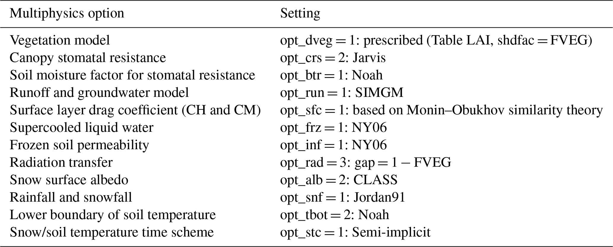
The multiphysics options of Noah-MP were set as shown in Table 1. For the simulation we used the US Geological Survey land use dataset. The vegetation type index was set to 2 (dryland cropland and pasture) and soil type index to 4 (silt loam). The model was forced with half-hourly weather data (wind speed, wind direction, temperature, humidity, pressure, precipitation, downwelling longwave and shortwave radiation) measured at EC1 from 2011 to 2012. Simulations were initialized with a spinup period of 1 year (2011) and run with a time step of 1800 s.
Table 1Settings of the multiphysics options used in the Noah-MP simulation.
2.3.2 GVF dynamics
The GVF data required by the Noah-MP model were derived from high-resolution (5 m × 5 m) RapidEye satellite data. Detailed information on the deriving of the GVF data used in the current research can be found in Imukova et al. (2015). The GVF data were calculated from the normalized difference vegetation index (NDVI) computed from the red and near-infrared bands of the satellite images. The relationship between the GVF and NDVI was established by linear regression using ground truth measurements. GVF maps for the Kraichgau region were derived at a monthly resolution.
Table 2GVF dynamics of early-covering crops (ECC) and late-covering crops (LCC) in 2012 and 2013 in the Kraichgau region, southwest Germany, as well as the GVF dynamics of the generic crop.

a Weighted mean GVF calculated based on fractions of ECC (72 %) and LCC (28 %) in Kraichgau. b No RapidEye scenes were available for April. c No RapidEye scenes were available for these months; GVF values were derived by linear interpolation between adjacent months.
Table 2 shows the observed and mean GVF dynamics of ECC and LCC over the growing seasons 2012 and 2013 as well as the GVF dynamics of the generic crop in the Kraichgau region. The GVF values on the 15th day of each month, as required by the Noah-MP model, were calculated by linearly interpolating the monthly values derived from the GVF maps. A generic GVF dynamic was calculated as the weighted mean of ECC and LCC from 2012 and 2013. The areal distribution of ECC and LCC was determined from the GVF maps of May 2012. All pixels with a GVF value below 0.5 were counted as LCC, whereas pixels with values above that threshold were assigned to ECC. Figure 1 shows the spatial distribution of early- and late-covering crops in Kraichgau. The estimated areal distribution of ECC and LCC was 72 % and 28 %, respectively. These results correspond well with data of the Statistisches Landesamt Baden-Württemberg (http://www.statistik.baden-wuerttemberg.de/, last access: November 2019).
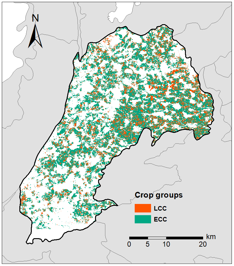
Figure 1Map of early-covering (ECC) and late-covering crops (LCC) in Kraichgau region, southwestern Germany.
2.3.3 LAI dynamics
Noah-MP requires prescribed LAI data for each month. Data were derived from field measurements. The LAI was measured biweekly using an LAI-2000 plant canopy analyzer (LI-COR Biosciences Inc., USA). In 2012 and 2013, the LAI of the crops was measured on five permanently marked plots of 1 m2 on three different fields. Detailed information about the study plots can be found in Imukova et al. (2015). In 2009–2011, the LAI and the phenological development of the crops were measured on five permanently marked plots of 4 m2 in the same three fields. The growth stages of crops were determined using the BBCH scale (Meier et al., 2009). More details on the measurements can be found in Ingwersen et al. (2011, 2015). Table 3 shows measured and mean LAI dynamics as well as generic LAI dynamics estimated by considering shares of ECC (72 %) and LCC (28 %) in the study region. LAI dynamics of winter wheat and winter rape were assigned to ECC; those of maize were assigned to LCC. The mean LAI dynamics of ECC were estimated based on the measurements conducted in winter wheat and winter rape stands during the 2012 and 2013 growing seasons. Since LAI data were not available for maize in 2013, the mean LAI dynamics of LCC were assessed using field data from the same fields collected in 2009–2012.
Table 3LAI dynamics of early-covering crops (ECC) and late-covering crops (LCC) in 2012 and 2013 in the Kraichgau region, southwest Germany, as well as the LAI dynamics of the generic crop.

a Weighted mean LAI calculated based on fractions of ECC (72 %) and LCC (28 %) in Kraichgau. b LAI data for maize in 2013 were not measured. c Since LAI data for maize in 2013 were not available, LAI dynamics were derived from the field data of 2009–2012 for maize in the Kraichgau region.
2.4 Simulation runs
We firstly quantified the extent to which ECC and LCC differ with regard to their energy and water fluxes, surface temperature (TS) and soil temperature (TG). For this, we performed one local simulation for each crop group using the mean LAI and the mean GVF dynamics observed during the two growing seasons (see Tables 2 and 3).
Secondly, to determine the effect of splitting up the vegetation dynamics of a generic crop into that of ECC and LCC, we compared the following two local simulation runs:
-
In Run 1, Noah-MP was forced with the GVF and LAI dynamics of the generic crop (Tables 2 and 3). Accordingly, in this simulation, we first computed the weighted mean of the vegetation properties (GVF and LAI) and subsequently simulated the surface energy fluxes, TS and TG.
-
In Run 2, we first simulated the energy and water fluxes separately for ECC and LCC with their crop-specific vegetation dynamics. Afterward, we calculated the weighted averages of the simulated fluxes and temperatures based on the share of early-covering (72 %) and late-covering crops (28 %) in Kraichgau.
Thirdly, we studied the effect of increasing the LCC share on the surface energy fluxes and surface and soil temperatures. As mentioned in the introduction, the maize cropping area in Germany increased by 53 % over the last decade. In Kraichgau currently 46 % of the total area is covered by croplands. Taking the above fractions of ECC and LCC results in areal fractions of ECC and LCC of 33 % and 13 %, respectively, of the total area. An increase in LCC at the expense of grassland increases LCC share from 13 % to 20 % and increases the areal fraction of croplands to 53 %, which leads to a rise in the share of LCC on croplands from 28 % to 38 %. To study the effect of this land use change on the Noah-MP simulations, we performed one additional generic crop simulation, but this time the generic crop dynamics were computed with an LCC share of 38 %.
2.5 Statistical analysis
The model performance was evaluated based on the model efficiency (EF), root-mean-square error (RMSE) and bias. EF is defined as the proportion of the total variance explained by a model:
where Pi denotes predicted values and Oi and are observed values and their mean, respectively, while N is the number of observations. RMSE and bias were calculated as
and
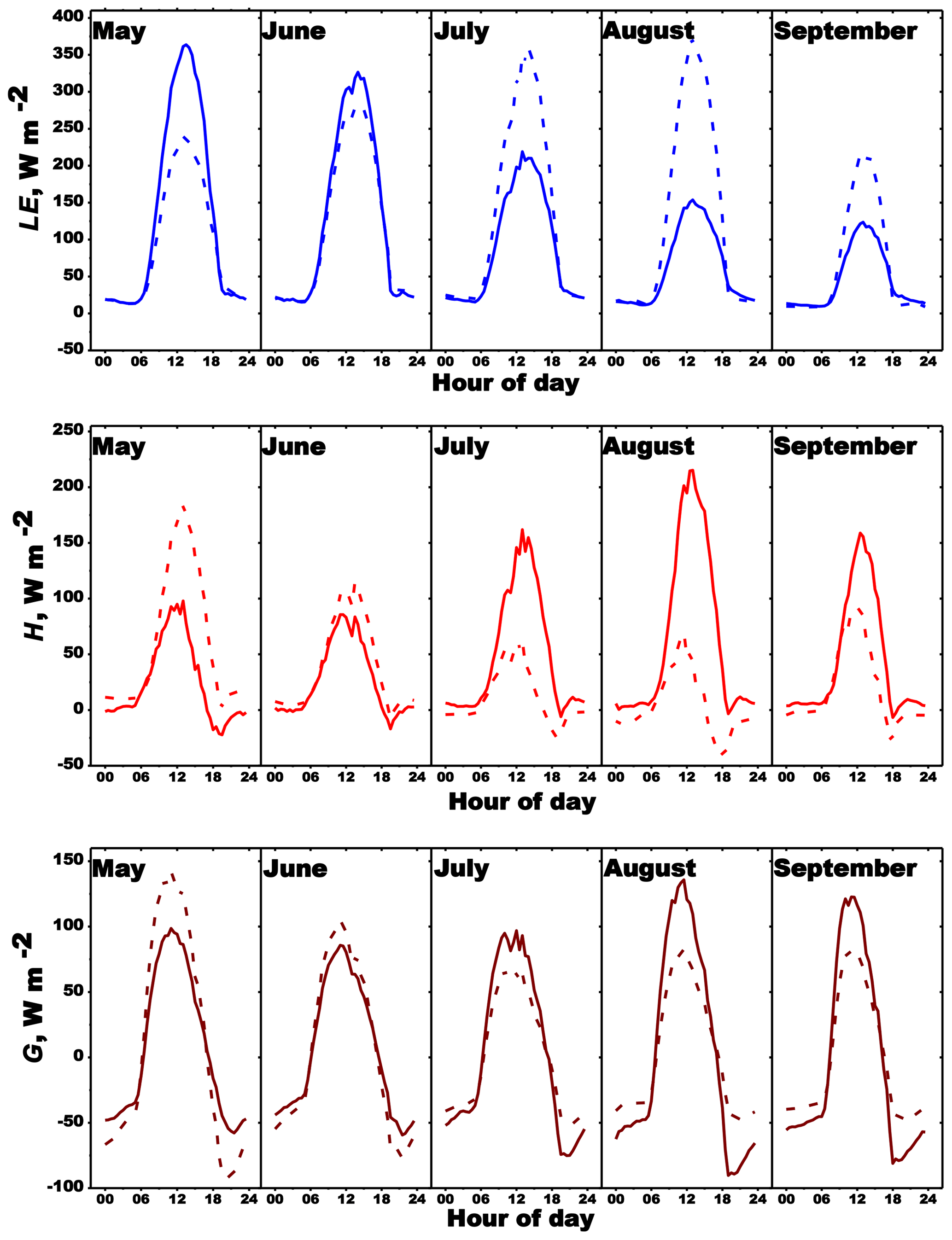
Figure 2Simulation results of Noah-MP LSM for latent heat flux (LE), sensible heat flux (H) and ground heat flux (G). Simulations were performed for two types of crops: early covering (solid line) and late covering (dashed line). Time is local time.
3.1 ECC vs. LCC
Over the growing season, ECC and LCC show distinct differences with regard to energy partitioning at the land surface (Fig. 2). The observed shifts were strongest for LE and H. Early-covering crops had already reached their maximum LE value in May, after which LE declined during the growing season. In contrast, LCC showed a continued increase in LE over the season, peaking 3 months later in August. The smallest difference in evapotranspiration between both crop types was on average 0.4 mm d−1 (LE 0.9 MJ m−2 d−1) in June, while the largest mean deviation of −2.3 mm d−1 (LE −5.7 MJ m−2 d−1) occurred in August (Table 4). With regard to H, the situation was opposite (Fig. 2). In the case of ECC, H increased continuously over the course of the growing season, peaking in August. In contrast, LCC had already reached the H maximum in May. Afterward, H decreased continuously until late August. As for LE, the smallest (−1.2 MJ m−2 d−1) and largest (5.3 MJ m−2 d−1) mean differences in H between ECC and LCC were observed in June and August, respectively (Table 4). Compared with LCC, the higher latent heat fluxes of ECC in May and June resulted in a cooler land surface, on average by −2.6 and −1.0 ∘C, respectively (Table 4). From July to August the situation was reversed: because latent heat fluxes of ECC are distinctly lower than that of LCC, the surface temperature at ECC sites was up to 4 ∘C warmer than at LCC sites (Fig. 3).
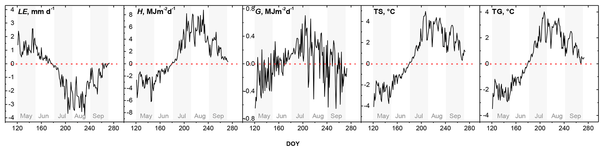
Figure 3Differences (ECC minus LCC) in latent heat flux (LE), sensible heat flux (H), ground heat flux (G) , mean surface temperature (TS) and mean ground temperature (TG) between simulations for ECC and LCC.
Table 4Mean differences (ECC minus LCC) in latent heat flux (LE), sensible heat flux (H), ground heat flux (G), mean surface temperature (TS) and mean ground temperature (TG) between ECC and LCC simulations.
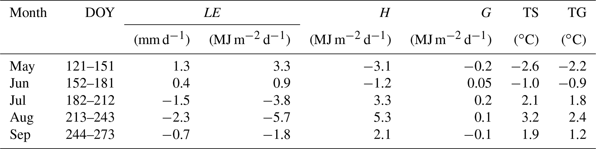
DOY is day of year.
The mean difference in daily ground heat flux between ECC and LCC during the growing season ranged between −0.2 and 0.2 MJ m−2 (Table 4). Also for the ground heat flux, the smallest difference between both crops types was observed in June (0.05 MJ m−2).
3.2 Noah-MP vs. eddy covariance measurements
The average random error of the latent heat flux measured with the EC technique for the entire growing season was about 25 % over the winter wheat field and about 21 % over the maize field.
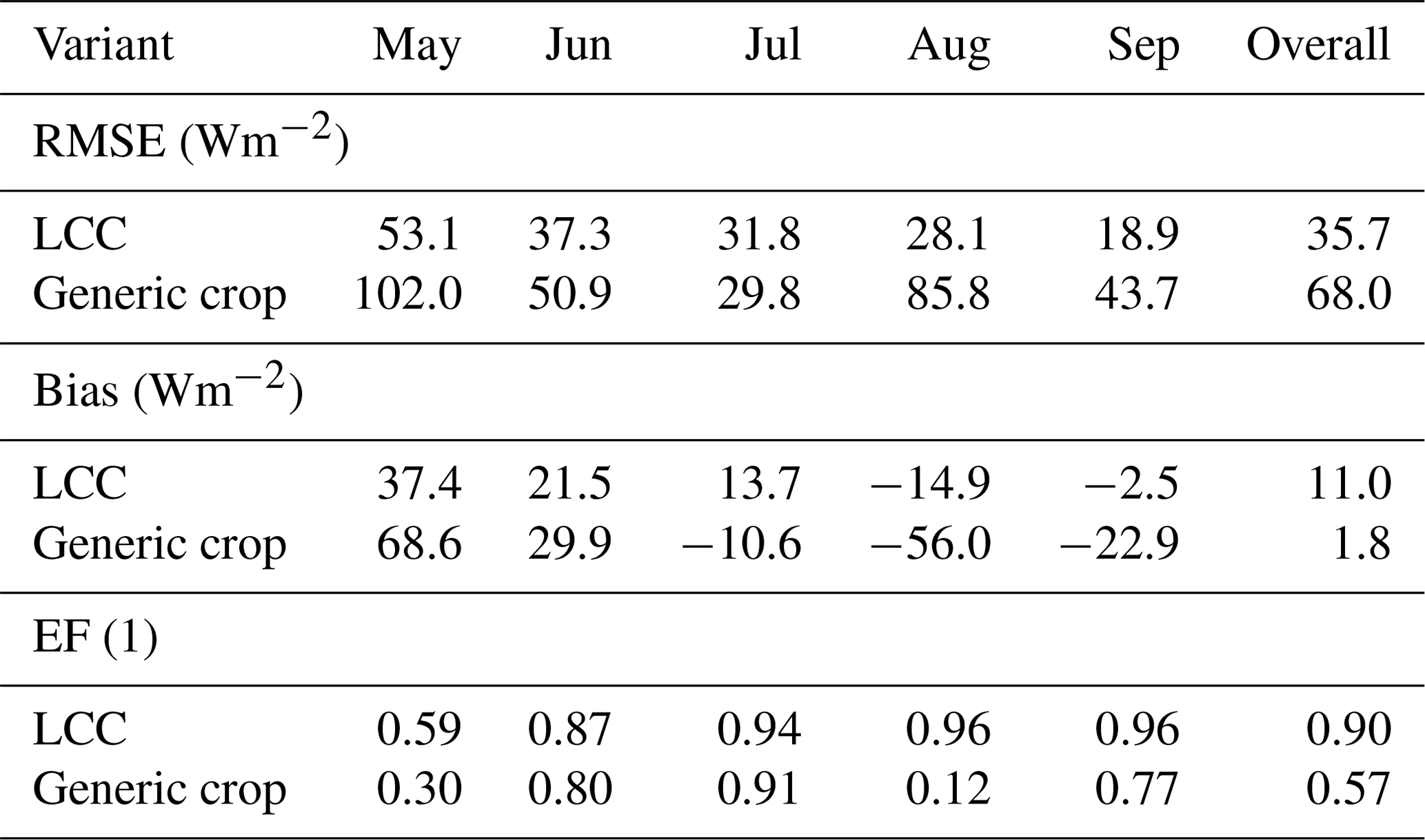
The simulated latent heat flux based on ECC and LCC parametrization agreed fairly well with the eddy covariance data (Tables 5–6, Figs. 4–5). The model efficiency over the entire simulation period was 0.87 for ECC and 0.90 for LCC. The best agreement between the observations and the Noah-MP LSM using crop-type-specific sets was achieved for winter wheat in June and for maize in August and September. The generic crop parametrization showed less satisfying modeling results, particularly for the maize field (Tables 5–6). For the entire growing season, EF was 0.78 for winter wheat and only 0.57 for maize. Over the winter wheat field, LE was overestimated. Overestimation of LE was highest in July and August. Over the maize field, LE was overestimated in May and June and underestimated in July, August and September. Particularly in May and August, the bias increased to 68.8 and −56 Wm−2, respectively. The best model performance using the generic crop set was achieved for the winter wheat in June and for the maize in July.
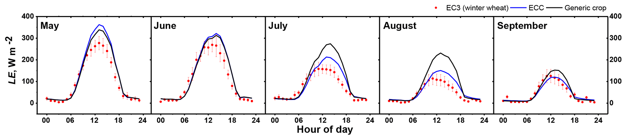
Figure 4Monthly averaged measured and simulated diurnal latent heat flux (LE) for May–September. The Noah-MP LSM was run with two different vegetation parametrizations: early-covering crops (ECC) and generic crop.
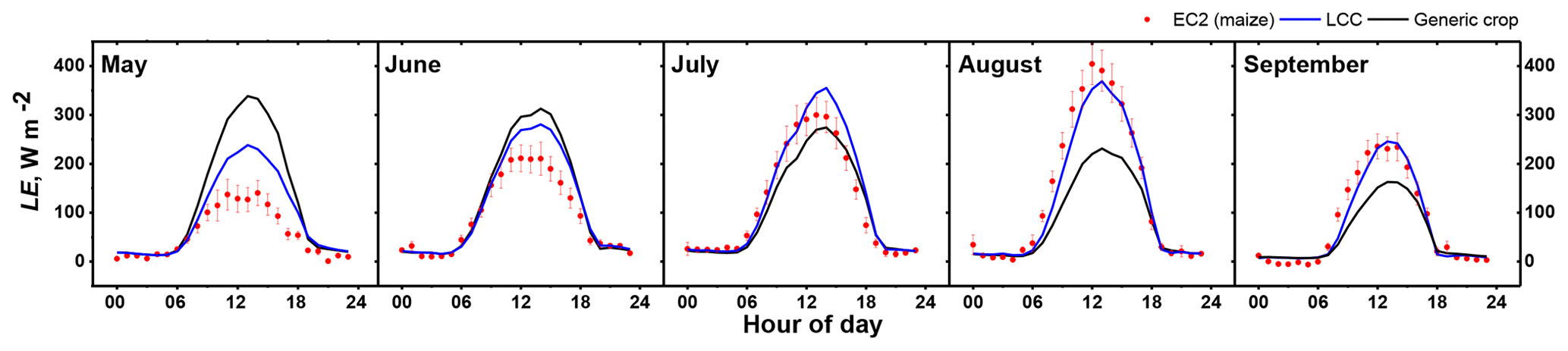
Figure 5Monthly averaged measured and simulated diurnal latent heat flux (LE) for May–September. The Noah-MP LSM was run with two different vegetation parametrizations: late-covering crops (LCC) and generic crop.
Table 5Root-mean-square error (RMSE), bias and modeling efficiency (EF) of the latent heat flux for the simulation runs of winter wheat stand (EC3 field).
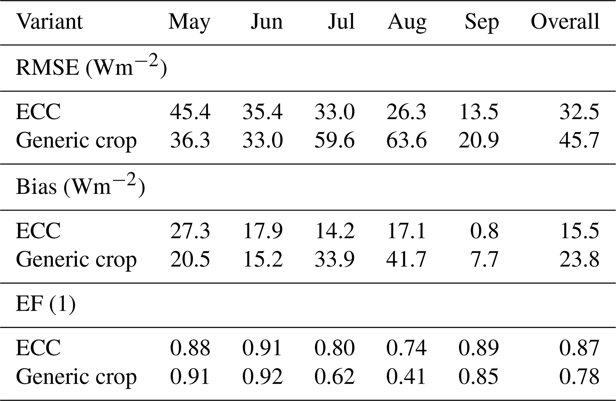
Table 6Root-mean-square error (RMSE), bias and modeling efficiency (EF) of the latent heat flux for the simulation runs of maize stand (EC2 field).
3.3 Run 1 vs. Run 2 (generic crop vs. weighted mean of ECC and LCC)
The generic crop simulation run (Run 1) generally yielded higher LE than Run 2 (i.e., splitting up the generic crop into ECC and LCC; Fig. 6). During the growing season the mean difference in evapotranspiration between two runs was 0.1 mm d−1 (LE 3.7 MJ m−2 d−1; Table 7). The smallest mean monthly differences occurred in June and September: 0.02 mm d−1 (LE 0.4 MJ m−2 d−1) and 0.03 mm d−1 (LE 1 MJ m−2 d−1), respectively. The most pronounced differences in LE were recorded in late July (DOY 197–208; Fig. 7). The average difference in half-hourly fluxes over this period, between 09:00 and 18:00 LT, was 36 W m−2, and the highest half-hourly deviation between both runs was 83 W m−2 (Fig. 7). The highest daily deviation was 0.8 mm d−1 (Fig. 6). Over the whole season, the cumulative difference in evapotranspiration between two runs was 20 mm, leading to a 16 % lower seasonal water balance (SWB) in Run 1 (SWB −133 mm) than in Run 2 (SWB −113 mm).
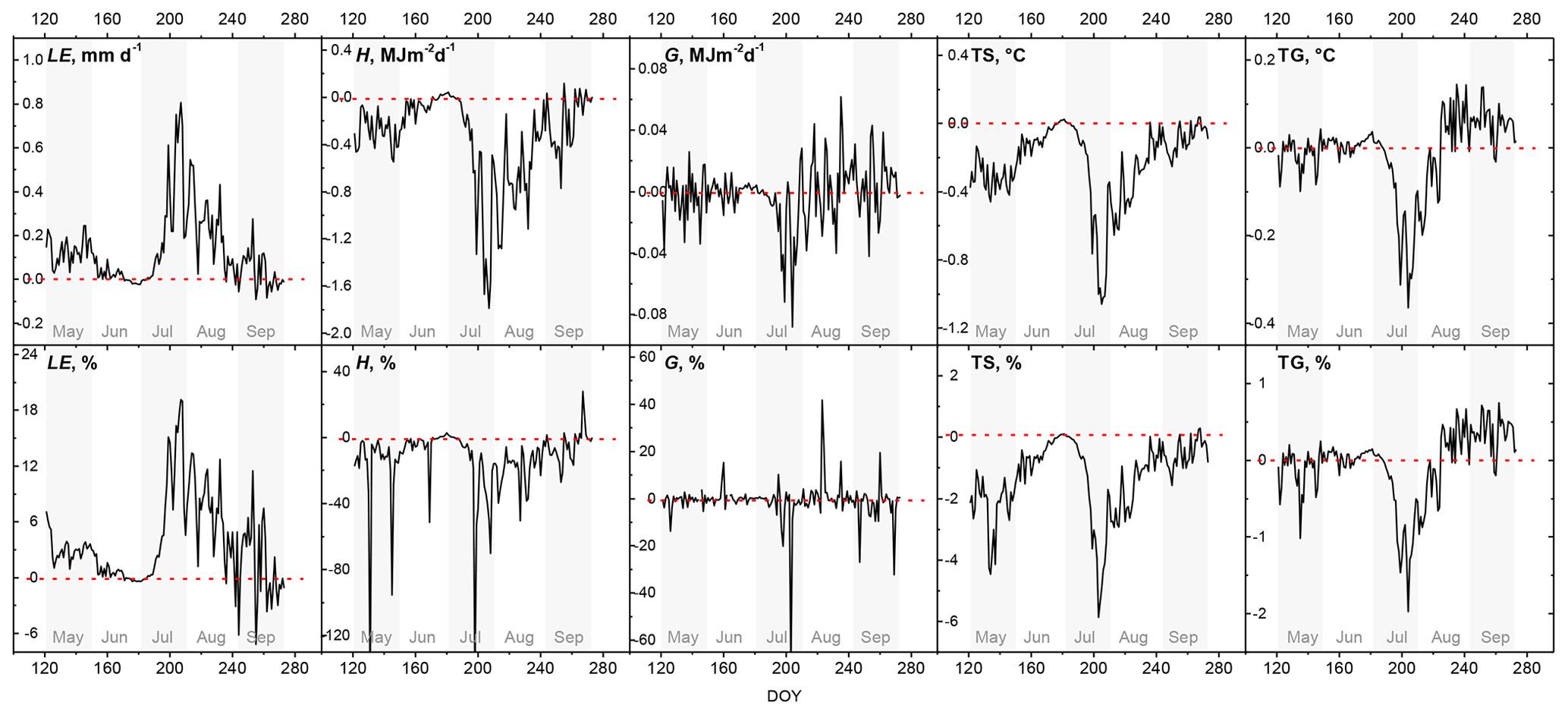
Figure 6Differences in latent heat flux (LE), sensible heat flux (H), ground heat flux (G), mean surface temperature (TS) and mean ground temperature (TG) between Run 1 and Run 2 simulations (Run 1–Run 2). Given percentages are relative differences between Run 1 and Run 2 simulations.
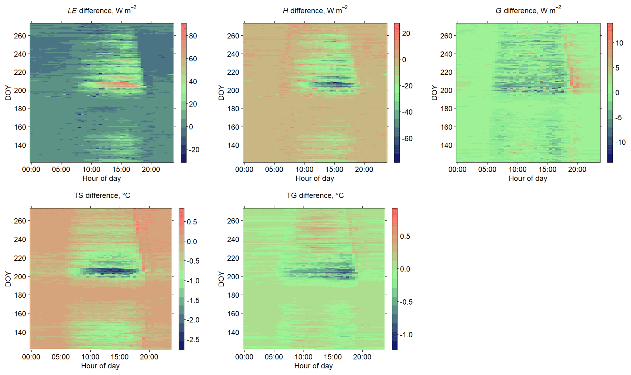
Figure 7Differences in latent heat flux (LE), sensible heat flux (H), ground heat flux (G), mean surface temperature (TS) and mean ground temperature (TG) between Run 1 (generic crop) and Run 2 (weighted mean of early- and late-covering crops) simulations (Run 1–Run 2). Time is local time.
Table 7Mean differences in latent heat flux (LE), sensible heat flux (H), ground heat flux (G), surface temperature (TS) and ground temperature (TG) between Run 1 and Run 2 simulations. Numbers in parentheses: the relative difference between Run 1 and Run 2 simulations as a percentage.
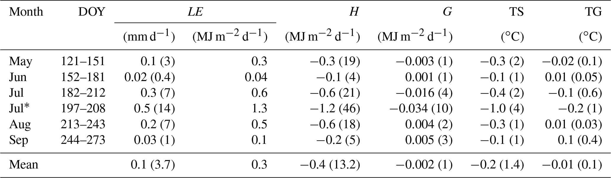
DOY is day of year. * 15–27 July.
In contrast, H values of Run 1 were mostly lower over all months than those simulated in Run 2 (Fig. 6). From May to September, the mean difference in H was about −0.4 MJ m−2 (−13 %; Table 7). The smallest difference occurred again in June; the largest difference occurred again in late July (Fig. 7). During DOY 197–208 the mean differences in half-hourly H values were about −29 W m−2, the peak deviation being −72 W m−2 (09:00–18:00 LT; Fig. 7). Cumulating these differences over the day reduced the production of sensible heat on average on the order of 1.2 MJ m−2, corresponding to a 46 % reduction compared to Run 2 (Table 7). Ground heat fluxes as well as soil temperature were affected only moderately by the different vegetation parametrization of Run 1 and 2 (Figs. 7, 6). As for LE and H, the largest mean differences in G values were observed during DOY 197–208 (−0.034 MJ m %; Table 7).
Due to the humid bias of Run 1, the canopy surface was cooler than in Run 2 in all months. On average, the TS of Run 1 was 0.2 ∘C (∼1.4 %) lower during the growing season than in Run 2. In late July (DOY 197–208) the mean daily difference was −1 ∘C (Table 7, Fig. 6) and reached a daytime (09:00–18:00 LT) peak difference of up to −2.6 ∘C (Fig. 7).
3.4 Land use change towards LCC
Increasing the LCC fraction from 28 % to 38 % mainly led to changes in LE and H (Table 8). That LCC increase lowered the LE value (−0.3 MJ m−2 d−1 or ET 0.1 mm d−1) early in the season. This was accompanied by a higher H value (+0.3 MJ m−2 d−1), which in turn led to a 0.3 ∘C warmer surface temperature than for the runs with the actual ECC / LCC ratio. From July to September, increasing the LCC fraction boosted evapotranspiration by about 0.2 mm d−1 (LE 0.4 MJ m−2 d−1) and decreased the H value by about 0.3 MJ m−2 d−1 (Table 8). The largest half-hourly differences occurred in August (DOY 213–243, Fig. 8), amounting to +40 and −30 W m−2 for LE and H, respectively. The smallest deviations for both fluxes were recorded in June. Over the July–September period, the higher LE value of the simulation run with the increased LCC fraction cooled the land surface by up to −1 ∘C (Fig. 8). In general over the growing season, increasing the LCC share by 10 % led to an increase in cumulative evapotranspiration, which in turn resulted in a 10 mm lower seasonal water balance (SWB −143 mm).
Table 8Mean differences in latent heat flux (LE), sensible heat flux (H), ground heat flux (G), surface temperature (TS) and ground temperature (TG) between simulations with the LCC fraction increased by 10 % and the baseline simulation (increased LCC share minus baseline simulation). Numbers in parentheses: the relative difference between increased LCC share and baseline simulation as a percentage.
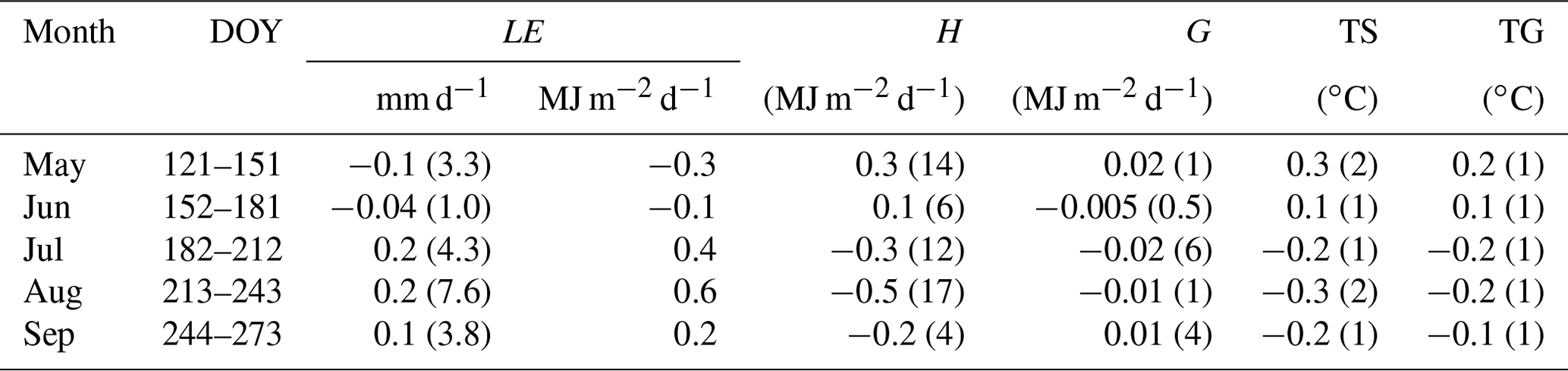
DOY is day of year.
With regard to the ground heat flux, increasing the LCC fraction led to an up to 10 W m−2 higher flux over the noontime during the second part of the growing season (Fig. 8), whereas early in the season the differences did not exceed 0.2 ∘C (Table 8).
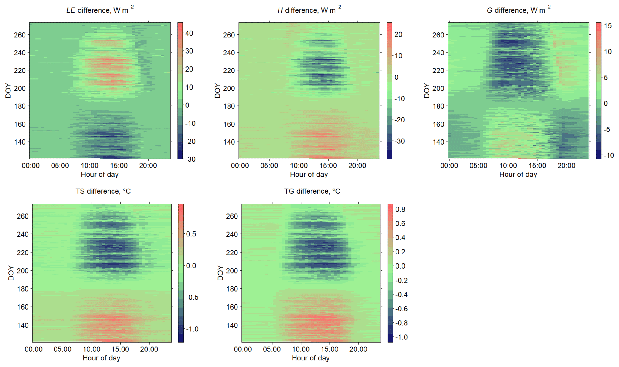
Figure 8Impact of increasing the LCC fraction from 28 % to 38 % on latent heat flux (LE), sensible heat flux (H), ground heat flux (G), surface temperature (TS) and ground temperature (TG) (increased LCC share minus baseline simulation). Time is local time.
The comparison of the ECC and LCC simulations confirmed that the GVF and LAI significantly affect the partitioning of surface energy fluxes. The LE value increases with crop growth and peaks when the canopy is fully developed, i.e., has a maximum LAI and GVF. By contrast, the highest H and G values were observed at sparsely covered fields or on the fields with a senescent canopy. During the main growth period of crops, H and G values were quite low. ECC and LCC vary significantly in sowing and harvest date, leaf area and senescence dynamics, water use efficiency, and phenology. Their surface energy fluxes therefore differ distinctly. Our simulation results are in agreement with experimental data of Wizeman et al. (2014) as well as with modeling studies of Sulis et al. (2015), Tsvetsinskaya et al. (2001b), Xue et al. (1996) and Ingwersen et al. (2018).
Simulation results based on ECC and LCC parametrization are in complete harmony with the field observations at our study site. The performance test of Noah-MP on the EC data showed the crop-type-specific sets significantly improve the simulation of latent heat flux at the field scale. In contrast, generic crop parametrization showed less satisfying modeling results. In general, it performed better for winter wheat stand than for maize. Based on the generic crop set, simulation results tend to greatly overestimate the latent heat flux for maize in the beginning of the growing season when the plants are small. In August and September, the latent heat flux was in contrast distinctly underestimated; during this period the maize canopy is fully developed. For wheat, the model overestimates the latent heat flux, particularly during the July–September period, when the winter wheat stand ripened and reached senescence or was harvested.
Besides the vegetation dynamics, the simulated energy and water fluxes depend on additional model settings. Ingwersen et al. (2011) performed a sensitivity study with the Noah model for our study site. They found that among the vegetation parameters the minimum stomatal resistance (RS) and a parameter used in the radiation stress function of the Jarvis scheme (RGL) are the most sensitive parameters. Using constant RS, as it is implemented in Noah, results in the underestimation of sensible heat flux and overestimation of latent heat flux during the ripening stage of the cereals. Considering a monthly varying RS helped to distinctly improve the simulation of the energy and water fluxes at the land surface. Ingwersen et al. (2010) concluded that integrating the crop growth model which delivers daily RS, LAI and GVF values into Noah would greatly enhance the overall performance of the land surface model. Among the soil parameters, the most sensitive parameters are the soil moisture threshold where transpiration begins to stress (REFSMC), maximum soil moisture content (MAXSMC) and soil moisture threshold where direct evaporation from the top layer ends (DRYSMC). Considering these parameters also has the potential to further improve simulation results.
The potential increase in the LCC fraction (driven by the high demand for biogas and forage production) leads to significant changes in the partitioning of the energy fluxes in croplands. In recent years the total area under maize in Germany has more than doubled. This corresponds to an approximately 10 % increase in the LCC fraction for the study region. In the early vegetation period, the altered ECC / LCC ratio leads to a decrease in evapotranspiration, an increase in H and a warmer cropland surface because, during that period, a higher fraction of fields is bare or sparsely covered with vegetation. In mid-June, the situation reverses. The higher share of LCC boosts LE, decreases H and lowers surface temperatures. The increased evapotranspiration over the growing season, in turn, leads to a lower seasonal water balance.
Comparing the generic crop simulation (Run 1) with the weighted mean of two separate simulations for ECC and LCC (Run 2) showed the largest difference over the second half of the growing season, particularly during late July and early August. In July, ECC become senescent: GVF drops sharply and the green LAI equals zero. In early August, ECC are usually harvested. In contrast, LCC have a developed ground-covering canopy during July–August. Leaves of these crops are still green in September. This transition period is very smooth in the case of the generic crop, resulting on average in about 14 % higher LE and in about 46 %, 10 % and 4 % lower H, G and surface temperature values, respectively, compared with Run 2.
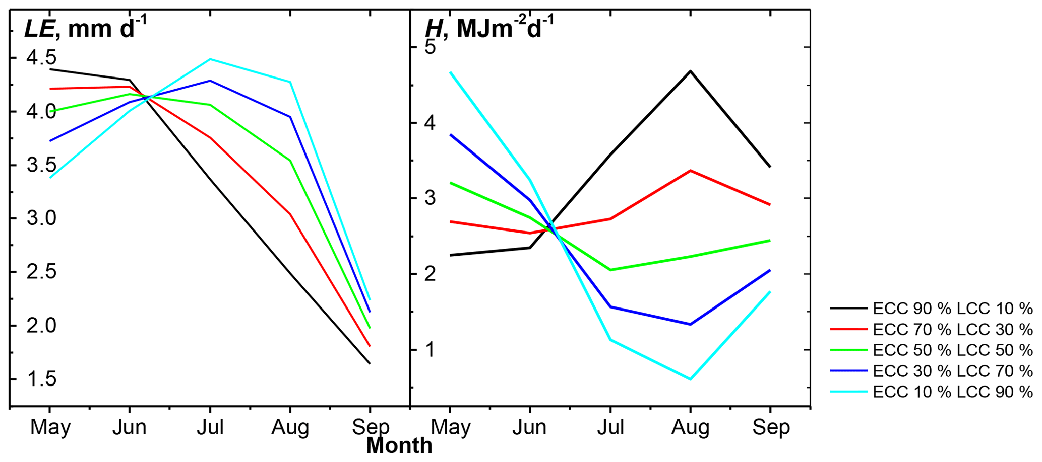
Figure 9Simulation results of Noah-MP LSM for latent heat flux (LE) and sensible heat flux (H). Simulations were performed considering different shares of ECC and LCC.

Figure 10Differences in latent heat flux (LE) and sensible heat flux (H) between Run 1 and Run 2 simulations (Run 1–Run 2). Simulations were performed considering different shares of ECC and LCC.
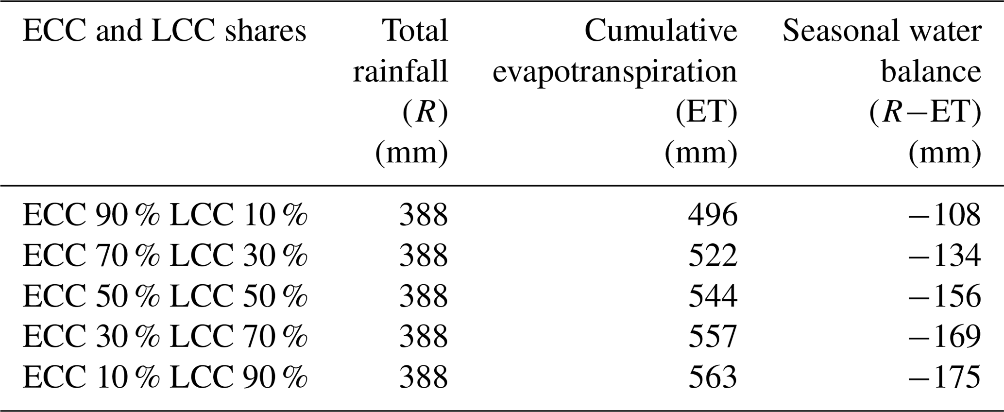
The results presented above apply to the ECC / LCC ratio within our study area. What can we expect in agricultural landscapes with different ECC / LCC ratios? The ECC / LCC ratio has nearly no effect on energy partitioning in June, whereas in May, July and August its influence on the turbulent fluxes is pronounced (Fig. 9). The weak effect in June is because, during this period, the LAI and GVF of ECC and LCC are similar (Fig. 11). In the other months, however, the ECC / LCC ratio heavily affects the energy partitioning. For example, increasing the LCC share from 10 % to 90 % boosts daily evapotranspiration in August from 2.5 to 4.3 mm d−1, decreases the H value by about 4.1 MJ m−2 d−1 and cools down the cropland surface by 2 ∘C. Over the growing season, the increase in the LCC share leads to a general increase in evapotranspiration, which in turn lowers the seasonal water balance (Table 9). Moreover, different ECC / LCC ratios will also affect the above-mentioned humid bias of the generic crop parametrization (Fig. 10). The bias is largest if ECC and LCC shares are balanced (ECC 50 % and LCC 50 %), whereas combinations with one predominant crop distinctly lower the bias. In August, for instance, the differences in LE between the two runs with ECC 50 %–LCC 50 % equal 0.27 mm d−1, while ECC 10 %–LCC 90 % yields differences of 0.09 mm d−1.
Table 9Weather data and simulation results of Noah-MP LSM for cumulative evapotranspiration for the Kraichgau region. Simulations were performed considering different shares of early-covering crops (ECC) and late-covering crops (LCC).
Our results show that performing simulations based on single dynamics for each type of crop (ECC and LCC) improve simulations of surface fluxes during transition periods and at the end of the growing season. Lumping ECC and LCC into one land-use class (croplands and pasture), as done in Noah-MP, is an oversimplification. Several authors have demonstrated the necessity to distinguish biophysical plant parameters in substantially different crops to obtain representative simulation results in the lower atmosphere (Sulis et al., 2015; Tsvetsinskaya et al., 2001b; Xue et al., 1996). They have showed that high-resolution spatial information on various croplands and associated physiological characterizations can significantly improve the simulations of land surface energy fluxes, leading to better weather and climate predictions.

Figure 11GVF and LAI dynamics of early-covering crops (ECC), late-covering crops (LCC) and cropland.
Changes in the LAI and GVF with plant growth lead to changes in surface albedo, bulk canopy conductance and roughness length, which in turn alter the partitioning of surface energy fluxes (Chen and Xie, 2011, 2012; Crawford et al., 2001; Tsvetsinskaya et al., 2001a; Xue et al., 1996). Such altered energy partitioning at the land surface then changes the thermodynamic state of the atmospheric boundary layer with regard to air temperature, surface vapor pressure, relative humidity and finally rainfall (Chen and Xie, 2012; McPherson and Stensrud, 2005; Sulis et al., 2015; Tsvetsinskaya et al., 2001b). The observed differences between Run 1 and crop-type-based runs will most probably influence the simulated processes in the ABL. For instance, Sulis et al. (2015) significantly improved the simulations of land surface energy fluxes by using the crop-specific physiological characteristics of the plant. They observed a difference of about 40 % between simulated fluxes using the generic and crop-specific parameter sets. The differences in the land surface energy partitioning led to different heat and moisture budgets of the atmospheric boundary layer for the generic and specific (sugar beet and winter wheat) croplands. In the case of specific croplands, particularly sugar beet, those authors observed a larger contribution of the entrainment zone to the heat budget of the ABL as well as a shallower ABL.
McPherson and Stensrud (2005) examined the impact of directly substituting the tallgrass prairie land use class with winter wheat on the formation of the ABL. These crops have different growing seasons. In the US Great Plains, native prairie tallgrass mainly grows in summer, while winter wheat grows throughout winter and reaches maturity in late spring. Simulations showed a larger LE value and lower H value over the area with the winter wheat stand in comparison with tallgrass. By 21:00 UTC, LE ranged from 300 to 400 W m −2 for the wheat run and from 200 to 275 W m −2 for the tallgrass run. H ranged from 25 to 125 W m −2 for the former and from 100 to 200 W m−2 for the latter. Substituting tallgrass prairie with winter wheat boosted the atmospheric moisture near the surface upstream and downstream of the study area, and resulted in a shallower ABL upstream and downstream of this area. The shallower ABL reduced the entrainment of higher-momentum air into the ABL and therefore led to weaker winds within the ABL.
Milovac et al. (2016) performed six simulations at a 2 km resolution with two local and two nonlocal ABL schemes combined with two LSMs (Noah and Noah-MP) to study the influence of energy partitioning at the land surface on the ABL evolution on a diurnal scale. They observed that LE values simulated by Noah-MP were more than 50 % lower than that simulated by Noah. As expected, a lower LE value resulted in a drier ABL. The ABL evolution and its features strongly influence the initiation of convection and cloud formation as well as the location and strength of precipitation. For instance, a drier and higher ABL would yield a higher lifting condensation level, leading to higher clouds and a higher probability of convective precipitation.
The GVF and LAI significantly affect the simulation of energy partitioning, yielding pronounced differences between simulated surface energy and water fluxes and temperatures of ECC and LCC. In our study area, the use of a generic crop parametrization (croplands and pasture in Noah-MP) resulted in a humid bias along with lower surface temperatures. This humid bias will be largest in landscapes with a balanced share of ECC and LCC, whereas in landscapes in which one of the two crop types predominate, the bias will be weaker. We observed the strongest effects on turbulent fluxes over the second part of the season, particularly in July–August. During this period, ECC are at the senescence growth stage or already harvested, while LCC have a fully developed ground-covering canopy. We therefore expect that the observed differences will impact the simulation of processes in the ABL. Our results show that splitting up croplands into ECC and LCC can improve LSMs, particularly during transition periods and late in the growing season.
Increasing the LCC fraction by 10 % reduces evapotranspiration and increases surface temperatures over the first part of the growing season. Later in the season, this land use change leads to the opposite situation: increased evapotranspiration accompanied by a slight cooling of the land surface. Over the growing season, an increase in the LCC share by 10 % leads to higher cumulative evapotranspiration, which in turn lowers the seasonal water balance.
Data is available at https://doi.org/10.1594/PANGAEA.916167 (Bohm et al., 2020).
The present study was a part of subproject P2, Soil–plant–atmosphere interactions at the regional scale, of the research unit 1695, Agricultural Landscapes under Global Climate Change – Processes and Feedbacks on a Regional Scale. TS is the primary investigator of this project and the supervisor of the present study. KB and experienced land surface modeler JI designed the modeling study. JM provided expertise in weather and climate modeling. KB performed the Noah-MP simulations and prepared the manuscript with contributions from all coauthors.
The authors declare that they have no conflict of interest.
This paper was edited by Paul Stoy and reviewed by two anonymous referees.
Bohm, K., Ingwersen, J., Milovac, J., and Streck, T.: Noah-MP simulated surface energy fluxes and temperature for a generic crop, early covering crops (ECC) and late covering crops (LCC) for Kraichgau region, southwest Germany, PANGAEA, https://doi.org/10.1594/PANGAEA.916167, 2020.
Chen, F. and Xie, Z.: Effects of crop growth and development on land surface fluxes, Adv. Atmos. Sci., 28, 927–944, 2011.
Chen, F. and Xie, Z.: Effects of crop growth and development on regional climate: A case study over East Asian monsoon area, Clim. Dynam., 38, 2291–2305, 2012.
Crawford, T. M., Stensrud, D. J., Mora, F., Merchant, J. W., and Wetzel, P. J.: Value of incorporating satellite-derived land cover data in MM5/PLACE for simulating surface temperatures, J. Hydrometeorol., 2, 453–468, 2001.
El Maayar, M., Chen, J. M., and Price, D. T.: On the use of field measurements of energy fluxes to evaluate land surface models, Ecol. Model., 214, 293–304, 2008.
Fachagentur Nachwachsende Rohstoffe e.V.: Anbau und Verwendung nachwachsender Rohstoffe in Deutschland, report number: FKZ 22004416, availabel at: http://www.fnrserver.de/ftp/pdf/berichte/22004416.pdf (last access: November 2019), 2019.
Falge, E., Baldocchi, D., Olson, R., Anthoni, P., Aubinet, M., Bernhofer, C., Burba, G., Ceulemans, R., Clement, R., Dolman, H., Granier, A., Gross, P., Grünwald, T., Hollinger, D., Jensen, N. -., Katul, G., Keronen, P., Kowalski, A., Lai, C. T., Law, B. E., Meyers, T., Moncrieff, J., Moors, E., Munger, J. W., Pilegaard, K., Rannik, Ü, Rebmann, C., Suyker, A., Tenhunen, J., Tu, K., Verma, S., Vesala, T., Wilson, K., and Wofsy, S.: Gap filling strategies for defensible annual sums of net ecosystem exchange, Agr. Forest. Meterol., 107, 43–69, 2001.
Ghilain, N., Arboleda, A., Sepulcre-Cantò, G., Batelaan, O., Ardö, J., and Gellens-Meulenberghs, F.: Improving evapotranspiration in a land surface model using biophysical variables derived from MSG/SEVIRI satellite, Hydrol. Earth Syst. Sci., 16, 2567–2583, https://doi.org/10.5194/hess-16-2567-2012, 2012.
Gutman, G. and Ignatov, A.: The derivation of the green vegetation fraction from NOAA/AVHRR data for use in numerical weather prediction models, Int. J. Remote Sens., 19, 1533–1543, 1998.
Huyghe, C., De Vliegher, A., van Gils, B., and Peeters, A.: Grassland and herbivore production in Europe and effects of common policies, Editions Quae, Versailles, 323 pp., https://doi.org/10.35690/978-2-7592-2157-8, 2014.
Imukova, K., Ingwersen, J., and Streck, T.: Determining the spatial and temporal dynamics of the green vegetation fraction of croplands using high-resolution RapidEye satellite images, Agr. Forest Meterol., 206, 113–123, 2015.
Imukova, K., Ingwersen, J., Hevart, M., and Streck, T.: Energy balance closure on a winter wheat stand: comparing the eddy covariance technique with the soil water balance method, Biogeosciences, 13, 63–75, https://doi.org/10.5194/bg-13-63-2016, 2016.
Ingwersen, J., Steffens, K., Högy, P., Warrach-Sagi, K., Zhunusbayeva, D., Poltoradnev, M., Gäbler, R., Wizemann, H.-D., Fangmeier, A., Wulfmeyer, V., and Streck, T.: Comparison of Noah simulations with eddy covariance and soil water measurements at a winter wheat stand, Agr. Forest Meterol., 151, 345–355, 2011.
Ingwersen, J., Imukova, K., Högy, P., and Streck, T.: On the use of the post-closure methods uncertainty band to evaluate the performance of land surface models against eddy covariance flux data, Biogeosciences, 12, 2311–2326, https://doi.org/10.5194/bg-12-2311-2015, 2015.
Ingwersen, J., Högy, P., Wizemann, H. D., Warrach-Sagi, K., and Streck, T.: Coupling the land surface model Noah-MP with the generic crop growth model Gecros: Model description, calibration and validation, Agr. Forest Meteorol., 262, 322–339, https://doi.org/10.1016/j.agrformet.2018.06.023, 2018.
Koster, R. D., Guo, Z., Dirmeyer, P. A., Bonan, G., Chan, E., Cox, P., Davies, H., Gordon, C. T., Kanae, S., Kowalczyk, E., Lawrence, D., Liu, P., Lu, C. H., Malyshev, S., McAvaney, B., Mitchell, K., Mocko, D., Oki, T., Oleson, K. W., Pitman, A., Sud, Y. C., Taylor, C. M., Verseghy, D., Vasic, R., Xue, Y., and Yamada, T.: GLACE: The Global Land-Atmosphere Coupling Experiment, Part I: Overview, J. Hydrometeorol., 7, 590–610, 2006.
Lhomme, J. T. and Chehbouni, A.: Comments on dual-source vegetation-atmosphere transfer models, Agr. Forest Meterol., 94, 269–273, 1999.
Margulis S. A. and Entekhabi, D.: Feedback between the Land Surface Energy Balance and Atmospheric Boundary Layer Diagnosed through a Model and Its Adjoint, J. Hydrometeorol., 2, 599–620, 2001.
Mauder M. and Foken. T.: Documentation and Instruction Manual of the Eddy-Covariance Software Package TK3, Arbeitsergebnisse Nr. 46, Universität Bayreuth, Abteilung Mikrometeorologie, Bayreuth, 60 pp., 2011.
Mauder, M., Cuntz, M., Drüe, C., Graf, A., Rebmann, C., Schmid, H. P., Schmidt, M., and Steinbrecher, R.: A strategy for quality and uncertainty assessment of long-term eddy-covariance measurements, Agr. Forest Meterol., 169, 122–135, 2013.
McPherson, R. A. and Stensrud, D. J.: Influences of a winter wheat belt on the evolution of the boundary layer, Mon. Weather Rev., 133, 2178–2199, 2005.
Meier, U., Bleiholder, H., Buhr, L., Feller, C., Hack, H., Hess, M., Lancashire, P. D., Schnock, U., Stauss, R., Van Den Boom, T., Weber, E., and Zwerger, P.: The BBCH system to coding the phenological growth stages of plants-history and publications, Journal für Kulturpflanzen, 61, 41–52, 2009.
Milovac, J., Warrach-Sagi, K., Behrendt, A., Späth, F., Ingwersen, J., and Wulfmeyer, V.: Investigation of PBL schemes combining the WRF model simulations with scanning water vapor differential absorption lidar measurements, J. Geophys. Res.-Atmos., 121, 624–649, 2016.
Nielsen, J. R., Ebba, D., Hahmann, A. N., and Boegh, E.: Representing vegetation processes in hydrometeorological simulations using the WRF model, DTU Wind Energy, (Riso – PhD; No. 0016(EN)), 128 pp., 2013.
Niu, G.-Y., Yang, Z.-L., Mitchell, K. E., Chen, F., Ek, M. B., Barlage, M., Kumar, A., Manning, K., Niyogi, D., Rosero, E., Tewari, M., and Xia, Y.: The community Noah land surface model with multiparameterization options (Noah-MP): 1. Model description and evaluation with local-scale measurements, J. Geophys. Res.-Atmos., 116, D12109, https://doi.org/10.1029/2010JD015139, 2011.
Raddatz, R. L.: Evidence for the influence of agriculture on weather and climate through the transformation and management of vegetation: Illustrated by examples from the Canadian Prairies, Agr. Forest Meterol., 142, 186–202, 2007.
Refslund, J., Dellwik, E., Hahmann, A. N., Barlage, M. J., and Boegh, E.: Development of satellite green vegetation fraction time series for use in mesoscale modeling: Application to the European heat wave 2006, Theor. Appl. Climatol., 117, 377–392, 2014.
Rundquist, B. C.: The influence of canopy green vegetation fraction on spectral measurements over native tallgrass prairie, Remote Sens. Environ., 81, 129–135, 2002.
Santanello Jr., J. A., Peters-Lidard, C. D., Kennedy, A., and Kumar, S. V.: Diagnosing the nature of land-atmosphere coupling: A case study of dry/wet extremes in the U.S. southern Great Plains, J. Hydrometeorol., 14, 3–24, 2013.
SRU Special Report: Climate Change Mitigation by Biomass, Special Report, The German Advisory Council on the Environment, available at: http://www.umweltrat.de/SharedDocs/Downloads/EN/02_Special_Reports/2007_Special_Report_Climate_Change.pdf?__blob=publicationFile (last access: November 2019), 2007.
Sulis, M., Langensiepen, M., Shrestha, P., Schickling, A., Simmer, C., and Kollet, S. J.: Evaluating the influence of plant-specific physiological parameterizations on the partitioning of land surface energy fluxes, J. Hydrometeorol., 16, 517–533, 2015.
Tsvetsinskaya, E. A., Mearns, L. O., and Easterling, W. E.: Investigating the effect of seasonal plant growth and development in three-dimensional atmospheric simulations. Part I: Simulation of surface fluxes over the growing season, J. Clim., 14, 692–709, 2001a.
Tsvetsinskaya, E. A., Mearns, L. O., and Easterling, W. E.: Investigating the effect of seasonal plant growth and development in three-dimensional atmospheric simulations. Part II: Atmospheric response to crop growth and development, J. Clim., 14, 711–729, 2001b.
van Heerwaarden, C. C., de Arellano, J. V.-G., Moene, A. F., and Holtslag, A. A. M.: Interactions between dry-air entrainment, surface evaporation and convective boundary-layer development, Q. J. R. Meteorol. Soc., 135, 1277–1291, 2009.
Wizemann, H.-D., Ingwersen, J., Högy, P., Warrach-sagi, K., Streck, T., and Wulfmeyer, V.: Three year observations of water vapor and energy fluxes over agricultural crops in two regional climates of Southwest Germany, Meteorol. Z., 24, 39–59, 2014.
Xue, Y., Fennessy, M. J., and Sellers, P. J.: Impact of vegetation properties on U.S. summer weather prediction, J. Geophys. Res.-Atmos., 101, 7419–7430, 1996.