Potential predictability of marine ecosystem drivers

Frölicher, Thomas L.; Ramseyer, Luca; Raible, Christoph C.; Rodgers, Keith B.; Dunne, John

doi:https://doi.org/10.5194/bg-17-2061-2020

Articles | Volume 17, issue 7

https://doi.org/10.5194/bg-17-2061-2020

Articles | Volume 17, issue 7

Research article

16 Apr 2020

Research article |

| 16 Apr 2020

Potential predictability of marine ecosystem drivers

Thomas L. Frölicher, Luca Ramseyer, Christoph C. Raible, Keith B. Rodgers, and John Dunne

Abstract

Climate variations can have profound impacts on marine ecosystems and the socioeconomic systems that may depend upon them. Temperature, pH, oxygen (O₂) and net primary production (NPP) are commonly considered to be important marine ecosystem drivers, but the potential predictability of these drivers is largely unknown. Here, we use a comprehensive Earth system model within a perfect modeling framework to show that all four ecosystem drivers are potentially predictable on global scales and at the surface up to 3 years in advance. However, there are distinct regional differences in the potential predictability of these drivers. Maximum potential predictability (>10 years) is found at the surface for temperature and O₂ in the Southern Ocean and for temperature, O₂ and pH in the North Atlantic. This is tied to ocean overturning structures with “memory” or inertia with enhanced predictability in winter. Additionally, these four drivers are highly potentially predictable in the Arctic Ocean at the surface. In contrast, minimum predictability is simulated for NPP (<1 years) in the Southern Ocean. Potential predictability for temperature, O₂ and pH increases with depth below the thermocline to more than 10 years, except in the tropical Pacific and Indian oceans, where predictability is also 3 to 5 years in the thermocline. This study indicating multi-year (at surface) and decadal (subsurface) potential predictability for multiple ecosystem drivers is intended as a foundation to foster broader community efforts in developing new predictions of marine ecosystem drivers.

How to cite

How to cite.

Dates

Received: 21 Dec 2019 – Discussion started: 08 Jan 2020 – Revised: 20 Mar 2020 – Accepted: 23 Mar 2020 – Published: 16 Apr 2020

1 Introduction

Marine organisms and ecosystems are strongly influenced by seasonal- to decadal-scale climate variations, challenging the sustainable management of living marine resources (Drinkwater et al., 2010; Lehodey et al., 2006). Anomalies in temperature, pH, O₂ and nutrients are important drivers of such climate-induced ecosystem variations (Gattuso et al., 2015; Gruber, 2011). Therefore, skillful predictions of these marine ecosystem drivers have considerable potential for use in marine resource management (Gehlen et al., 2015; Hobday et al., 2016; Payne et al., 2017; Tommasi et al., 2017).

The primary tools for investigating how marine organisms and ecosystems change on seasonal to decadal timescales are Earth system models, where prognostic equations are implemented for biogeochemical cycles. These models are capable of representing both natural variability and transient changes in the marine ecosystem drivers (Bopp et al., 2013; Frölicher et al., 2016). Recently, Earth system models have been used to explore and quantify the predictability of marine biogeochemical tracers. Most of the studies focus on predicting the ocean uptake of carbon (Li et al., 2016, 2019; Lovenduski et al., 2019; Séférian et al., 2018).

To date, only a few studies have investigated the predictability of marine ecosystem drivers (Chikamoto et al., 2015; Park et al., 2019; Séférian et al., 2014a). An intriguing finding of these studies is that marine biogeochemical drivers may be more predictable than their physical counterparts. Séférian et al. (2014a), for example, showed that net primary productivity (NPP) has greater predictability than sea surface temperature (SST) in the eastern equatorial Pacific. They hypothesized that SST is strongly influenced by high-frequency surface fluxes, whereas NPP is more directly impacted by thermocline adjustment processes that determine the rate at which nutrients are brought into the ocean's euphotic layer. Thus, biogeochemical predictions may hold great promise and highlight the need for further investigation. Changes in ecosystem drivers have impacts not only on the surface ocean but also over upper ocean waters spanning the euphotic zone and below, making it important to understand more broadly how ecosystem drivers vary over a range of depths. To our knowledge there is no comprehensive assessment of potential predictability of marine ecosystem drivers at the global scale spanning multiple depth horizons and a comparison of the relative predictability among them.

In this study, we assess the potential predictability of the four marine ecosystem drivers using “perfect model” simulations of a comprehensive Earth system model. We address the following three questions:

To what extent are marine ecosystem drivers predictable at the global scale?
What are the regional and depth-dependent characteristics of potential predictability?
Which underlying physical and biogeochemical processes prescribe or limit the potential predictability of marine ecosystem drivers?

This study is organized as follows. First, we introduce the model and methods used to assess the potential predictability in marine ecosystem drivers. Subsequently, the temporal sequencing of potential predictability over global scales for the four marine ecosystem drivers are identified and evaluated for regional differences in potential predictability horizons. Both surface and subsurface manifestations are presented to assess the origin of potential predictability. Finally, we also identify the mechanistic controls on the limits to potential predictability and conclude with a discussion and summary section.

2 Methods

2.1 Earth system model: GFDL-ESM2M

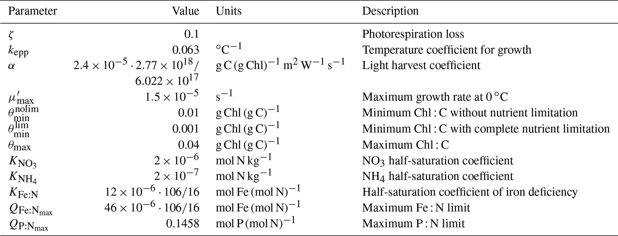
For this study we conducted a new 240-member ensemble suite of simulations of 10-year duration each with the Earth system model ESM2M developed at the Geophysical Fluid Dynamics Laboratory (GFDL) of the National Oceanic and Atmospheric Administration (NOAA; Dunne et al., 2012, 2013). The GFDL-ESM2M is a fully coupled carbon cycle–climate model. The physical core of the model is based on the physical coupled model CM2.1 (Delworth et al., 2006). The atmospheric model AM2 has a horizontal resolution of 2^∘ latitude × 2.5^∘ longitude with 24 vertical levels (Anderson et al., 2004). The land model simulates land water, energy and the carbon cycle, and it has the same horizontal resolution as the atmospheric component. The ocean model MOM4p1 (Griffies, 2012) has 50 vertical levels of varying thickness and a nominal horizontal resolution of 1^∘ latitude × 1^∘ longitude, increasing towards the Equator to up to 1∕3^∘. The sea ice model includes full ice dynamics, three thermodynamic layers and five ice thickness categories and is defined on the same grid as the ocean model (Winton, 2000).

Ocean biogeochemistry and ecology is simulated by the Tracers Of Phytoplankton with Allometric Zooplankton version 2.0 (TOPAZ2; Dunne et al., 2013). TOPAZ2 represents 30 prognostic tracers to describe the cycles of carbon, phosphorus, silicon, nitrogen, iron, alkalinity, oxygen and lithogenic material as well as surface sediment calcite. TOPAZ2 includes three phytoplankton functional groups: small (mostly prokaryotic pico- or nanoplankton), diazotroph (fixing nitrogen from the atmosphere) and large phytoplankton. TOPAZ2 only implicitly simulates zooplankton activity. The growth of phytoplankton depends on the level of photosynthetically active irradiance, nutrients (e.g., nitrate, ammonium, phosphate and iron) and temperature (see Sect. 2.3.2 and Appendix A).

Previous studies have shown that the GFDL-ESM2M captures the observed large-scale biogeochemical patterns (Dunne et al., 2012, 2013). The GFDL CM2.1 skillfully simulates primary modes of natural climate variability (Wittenberg et al., 2006) and has been extensively applied to assess seasonal and multiannual climate predictions (Meehl et al., 2013; Park et al., 2019).

2.2 Perfect model framework

We estimated potential predictability within a perfect model experiment. By perturbing the initial conditions of the GFDL-ESM2M and quantifying the spread of initially close model trajectories, the limit of initial condition predictability was assessed. The underlying assumption is that we have a perfect model (e.g., the model accurately represents all physical and biogeochemical processes relevant to assess marine ecosystem drivers at adequate temporal and spatial resolution) and nearly perfect initial conditions and that we exclude the role for external forcing in determining or limiting predictability. Specifically, we first performed a 300-year preindustrial control simulation (black line in Fig. 1), which is branched off a preexisting quasi-steady-state 1000-year preindustrial control simulation. Using this 300-year preindustrial control simulation to provide initial conditions, six 40-member ensemble simulations of 10-year duration each are performed. Each ensemble simulation starts at different times in the control simulation: 1 January in years 22, 64, 106, 170, 232 and 295. The six distinct initialization dates for the individual large ensemble simulations were randomly selected from the 300-year preindustrial control simulation. This was intended to average across biases that may result from predictability being different across different phases of climate modes (e.g., different El Niño–Southern Oscillation phase states) within the preindustrial simulation. Note that the last ensemble exceeds the control simulation by 5 years. Each of the six ensembles consists of 40 ensemble members with micro-perturbations to oceanic initial states but with the same atmospheric, land, ocean biogeochemical, sea ice and iceberg initial conditions. Specifically, for each ensemble member, i=1, 2, ..., 40, an infinitesimal temperature perturbation δ is added to a single grid cell in the Weddell Sea at 5 m depth, similar to the approach described in Wittenberg et al. (2014) and Palter et al. (2018):

\begin{matrix} (1) & δ_{i} = 0.0001^{\circ} C \times \{\begin{cases} \frac{i + 1}{2} : & for odd i \\ - \frac{i}{2} : & for even i \end{cases} . \end{matrix}

Thus, the range of perturbations is evenly spread from −0.002 to 0.002 ^∘C with the unperturbed control case in the center with zero perturbation. As stated above, our model setup encompasses 240 ensemble members, each of 10-year duration and thus 2400 years of model integration in addition to the 300-year-long control simulation. While our perturbation method is in no way optimal in terms of, for example, sampling the likely range of atmospheric–ocean–biogeochemical errors, it is sufficient to generate ensemble spread on the timescales of interest. After just 4 d of simulation time subsequent to the micro-perturbations for each cluster of 40 starting points, the SSTs of all surface ocean grid cells are numerically different from the SST of the control simulation, underscoring the rapidity with which divergences due to nonlinearities in the model express themselves. The method applied here mirrors that of Griffies and Bryan (1997a), Msadek et al. (2010), and Wittenberg et al. (2014) and emphasizes the amplitude (but not the phase) of perturbations to identify potential predictability. Our perturbation method produces ensemble experiments likely to give the upper limit of the model predictability, hence the term potential predictability. Nevertheless, it warrants mentioning here that studies have been published arguing that predictability in the real world for some variables may even be larger than estimated with the perfect modeling framework within an Earth system model in cases where the ratio of the predictable mode to model noise is underestimated (Eade et al., 2014; Kumar et al., 2014).

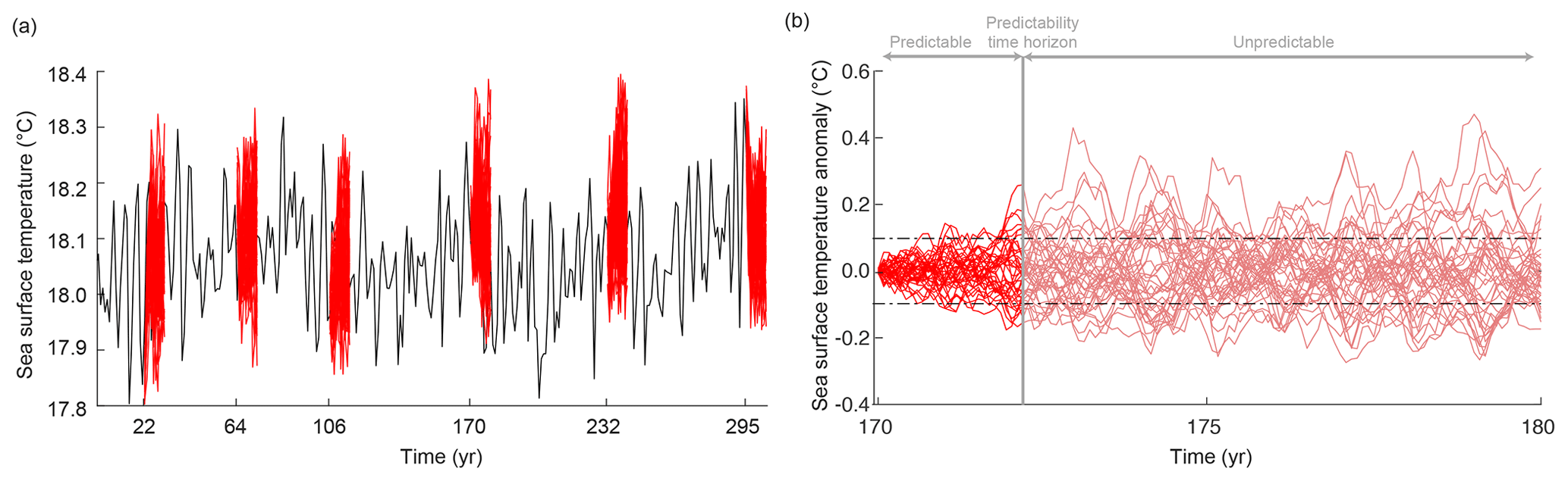
https://www.biogeosciences.net/17/2061/2020/bg-17-2061-2020-f01

Figure 1Illustration of the model setup and the calculation of the predictability time horizon. (a) Simulated global mean SST of the 300-year reference control simulation (black line) and of the six 10-year-long 40 ensemble simulations (red lines). (b) Global mean SST anomaly (i.e., deviation from the control simulation) for the ensemble simulation starting in the year 170. The thick red line indicates the period over which SST is predictable (i.e., PPP ≥0.183), and thin red lines indicate the period over which SST is unpredictable (i.e., PPP <0.183). The dashed horizontal lines indicate 1 standard deviation of the control simulation, and the vertical line indicates the predictability time horizon.

Download

2.3 Analysis methods

We calculate the potential predictability for the four marine ecosystem drivers: temperature, pH, O₂ and NPP. In the following, NPP is always integrated over the upper 100 m, whereas temperature, pH and O₂ are analyzed at different depth levels. In addition to identifying the upper limits of predictability of these variables within the Earth system model, an equally important objective is to identify the relative predictability of the four variables under consideration.

2.3.1 Assessment of potential predictability

The prognostic potential predictability (PPP) is the main metric used in this study to assess predictability. The PPP is the ratio between the variance among the ensemble members at a given time t after the initialization and the temporal variance of an undisturbed control simulation. The PPP is calculated following Griffies and Bryan (1997b) and Pohlmann et al. (2004):

\begin{matrix} (2) & PPP (t) = 1 - \frac{\frac{1}{N (M - 1)} \sum_{j = 1}^{N} \sum_{I = 1}^{M} {(X_{i j} (t) - {\overline{X}}_{j} (t))}^{2}}{σ_{c}^{2}}, \end{matrix}

where X_ij is the value of a given variable for the jth ensemble and ith ensemble member, ${\overline{X}}_{j}$ is the mean of the jth ensemble over all ensemble members, $σ_{c}^{2}$ is the variance of the control simulation, N is the total number of different ensemble simulations (N=6) and M the number of ensemble members (M=40). The variance of the control simulation is calculated for each month of the year separately to exclude the seasonality from the natural variability, i.e., only the natural variability at that month in the seasonal cycle is considered. PPP equal to unity constitutes perfect predictability. An F test is applied to estimate a significant difference between the ensemble variance and the variance of the control run. With N=6 and M=40, predictability is achieved with a 95 % confidence level when PPP ≥0.183.

The predictability time horizon is defined as the lead time at which PPP falls below the predictability threshold (Fig. 1b). To calculate global means, all metrics are first calculated at each individual grid cell and then averaged with area weighting over the global ocean.

2.3.2 Taylor deconvolution method to identify mechanistic controls of predictability

To understand the processes behind the simulated predictability, we applied a first-order Taylor-series deconvolution method to decompose the normalized ensemble variance of pH, O₂ and NPP into contributions from their physical and biogeochemical driver variables:

\begin{matrix} (3) & σ_{f}^{2} ≅ \sum_{i = 1}^{n} {(\frac{\partial f}{\partial x_{i}}| σ_{x_{i}})}^{2} + 2 \sum_{i < j} \frac{\partial f}{\partial x_{i}}| \frac{\partial f}{\partial x_{j}}| Cov (x_{i} x_{j}), \end{matrix}

where σ denotes the standard deviation among the ensemble members of the different variables. Specifically, the Taylor deconvolution method is applied to decompose the normalized ensemble variance for f of pH, O₂ and NPP into the contribution from their physical and biogeochemical drivers by expressing the ensemble variance and the variance of the control run from Eq. (2) in terms of Eq. (3). The partial derivatives in Eq. (3) are calculated at the point p=x, where x is the mean value of the corresponding driver variables over the entire control simulation.

The changes in pH are attributed to changes in temperature, salinity, total alkalinity (Alk) and total dissolved inorganic carbon (DIC). Here, we assume that variations in phosphate and silicate are negligible.

Dissolved oxygen (O₂) is decomposed into an oxygen solubility component $O_{2}^{sol}$ and an apparent oxygen utilization (AOU) component using (e.g., Frölicher et al., 2009)

\begin{matrix} (4) & O_{2} = {O_{2}}^{sol} - AOU . \end{matrix}

$O_{2}^{sol}$ is the solubility of oxygen, which depends nonlinearly on temperature and salinity (Garcia and Gordon, 1992). The difference between diagnosed $O_{2}^{sol}$ and simulated O₂ is AOU. Variations in AOU reflect changes in oxygen consumption and ocean ventilation. Earlier studies demonstrated that changes in AOU are typically associated with changes in ventilation, as simulated changes in the remineralization rates of organic material and in associated O₂ consumption are relatively small (Gnanadesikan et al., 2012).

NPP can be decomposed into the contributions from the three phytoplankton groups simulated in the TOPAZ2 model:

\begin{matrix} (5) & NPP = {NPP}_{Sm} + {NPP}_{Di} + {NPP}_{Lg}, \end{matrix}

where NPP_Sm, NPP_Di and NPP_Lg are the contributions from small, diazotroph and large phytoplankton, respectively. At any time t the NPP for all phytoplankton groups “phyto” is given by the phytoplankton stock P_phyto times the phytoplankton growth rate μ_phyto:

\begin{matrix} (6) & {NPP}_{phyto} (t) = μ_{phyto} (t) \cdot P_{phyto} (t) . \end{matrix}

The growth rate μ_Sm of the small phytoplankton is parameterized using a maximum growth rate μ_max, which is limited by nutrients N_lim, light L_lim and temperature T_f (see Appendix A for further details):

\begin{matrix} (7) & μ = μ_{max} \cdot N_{\lim} \cdot L_{\lim} \cdot T_{f} . \end{matrix}

Note that grazing, sinking and other loss processes impact phytoplankton stock, but these processes in TOPAZ2 are only a function of steady-state growth and biomass implicit grazing formulation, and they exert no separate dynamic control. Therefore they do not require separate consideration.

3 Results

3.1 Potential predictability at the ocean surface

The change in globally averaged annual PPP over time is very similar for all four marine ecosystem drivers at the surface, i.e., the PPP decreases exponentially over lead time for all four drivers (solid thick lines in Fig. 2). After 3 years, the PPP falls below the predictability threshold (dashed line in Fig. 2), indicating that the global predictability time horizon is about 3 years for all four ecosystem drivers. The seasonality in PPP (solid thin lines in Fig. 2) as well as the differences among the four drivers are very small at the global scale.

https://www.biogeosciences.net/17/2061/2020/bg-17-2061-2020-f02

Figure 2Globally averaged prognostic potential predictability (PPP) for all four marine ecosystem drivers at the surface, except for NPP which is integrated over the top 100 m. Monthly mean (thin lines) and annual mean (thick lines) values of PPP are shown. The horizontal black dashed line represents the predictability threshold. If PPP is above (below) the predictability threshold, the driver is potentially predictable (unpredictable) as indicated with the arrows on the right-hand side. The PPP has first been calculated at each grid cell and then averaged globally.

Download

https://www.biogeosciences.net/17/2061/2020/bg-17-2061-2020-f03

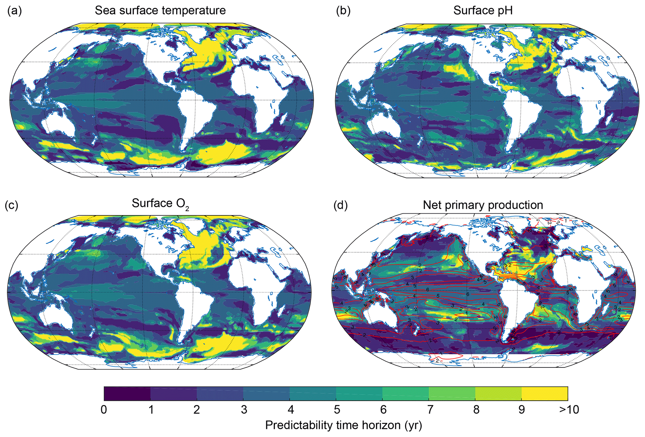
Figure 3Predictability time horizon for (a) SST, (b) surface pH, (c) surface O₂ and (d) NPP integrated over the top 100 m using PPP as a predictability measure. The red contour lines in panel (d) indicate the annual mean total nitrogen production in moles of nitrogen per kilogram per year averaged over the 300-year preindustrial control simulation to highlight regions with low and high NPP. In panel (d) regions north of 69^∘ N and south of 69^∘ S have been excluded since NPP is zero during wintertime there.

At the regional scale, the predictability time horizon shows distinct structured patterns and also large differences between each of the four different marine ecosystem drivers (Fig. 3). In general, SST (Fig. 3a), surface pH (Fig. 3b) and surface O₂ (Fig. 3c) share similar predictability time horizon patterns with short predictability time horizons (1–2 years) between 20 and 40^∘ in both hemispheres, intermediate predictability time horizons (3–5 years) in the tropical oceans, and long predictability time horizons (>10 years) in the North Atlantic between 40 and 70^∘ N, in the Southern Ocean between 40 and 65^∘ S (except for surface pH) and in the Arctic Ocean. Interestingly, the potential predictability time horizon of surface pH is short relative to SST and surface O₂ in the Southern Ocean but longer over both the Caribbean and the eastern subtropical North Pacific relative to SST. The Caribbean and the eastern North Pacific are both regions of importance for resource management, given the high density of neighboring human populations.

The NPP predictability time horizon pattern (Fig. 3d) is fundamentally different from the patterns of the other three ecosystem drivers. NPP has long predictability time horizons (6–10 years) in the midlatitudes, where the annual mean NPP is generally small (indicated with contour lines in Fig. 3d), but very short predictability time horizons of 0–1 years in the Southern Ocean, the North Atlantic and the Pacific, as well as short predictability time horizons of 1–3 years in the tropical oceans, where annual mean NPP is high (Fig. 3d). The spatial pattern of the predictability time horizon and the sequencing of predictability among the ecosystem drivers is very similar when using two other metrics for potential predictability, indicating that our results do not depend on the predictability metric used (Appendix B).

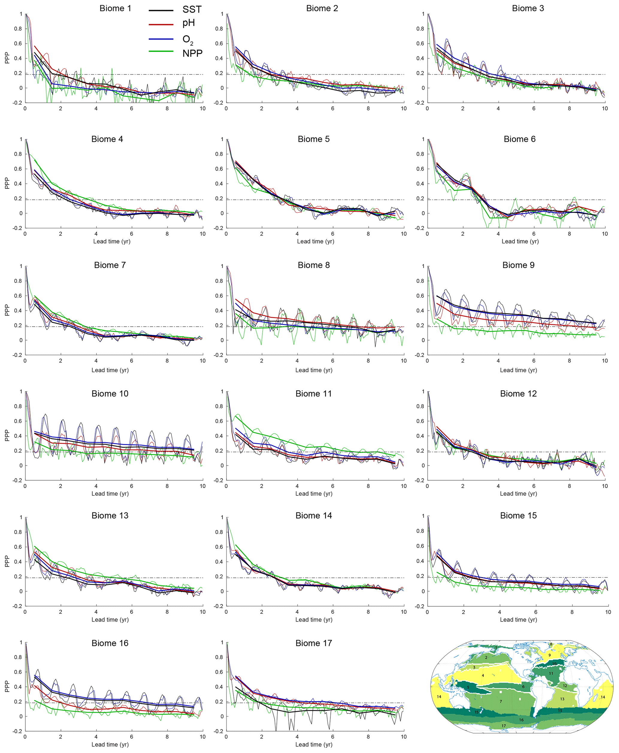
https://www.biogeosciences.net/17/2061/2020/bg-17-2061-2020-f04

Figure 4PPP for all four ecosystem drivers averaged over 17 different biomes at the surface, except for NPP, which is integrated over the top 100 m. Monthly means are shown as thin lines, and annual means are shown as thick lines. The horizontal dashed black lines in each panel represent the predictability threshold. The lower right panel shows the boundaries and the geographical location of biomes 1 to 17.

We further average the local potential predictability across 17 biogeographical biomes (Fig. 4) to highlight the pronounced seasonal cycle in predictability for some variables in particular biomes. The biomes capture patterns of large-scale biogeochemical function at the basin scale and are defined by distinct SSTs, maximum mixed-layer depths, maximum ice fractions and summer chlorophyll concentrations (Fay and McKinley, 2014). As shown in Fig. 4, potential predictability exhibits strong seasonality for SST, surface O₂ and surface pH in the North Atlantic (biomes 8, 9, 10 and 11), in the Southern Ocean (biomes 15 and 16) and in the subtropical/subpolar gyre boundary region of the North Pacific (biome 3). In all these biomes, predictability is higher during the cold season (boreal and austral winter) and lower during the warm season. The biomes with high seasonality in PPP are also the regions which generally show larger predictability in the annual mean. The PPP values of SST and surface O₂ have almost identical seasonal amplitudes, while the seasonal amplitude of the surface pH is generally smaller compared to SST and surface O₂ seasonal amplitude. Interestingly, the PPP for NPP generally shows no large differences amongst the seasons, except in biome 8, which is influenced by seasonal sea ice retreat and growth. Figure 4 also reveals other interesting characteristics of PPP. For example, the changes in PPP over lead time are very small, but they fluctuate around the predictability threshold for NPP in biome 10 and for SST and O₂ in biome 8, making the predictability horizon in some biomes for some variables very sensitive to small changes in PPP. In addition, the PPP for NPP in the eastern equatorial Pacific (biome 6) shows large interannual variations with lead time, indicating that even more ensemble members are needed to robustly assess the predictability there. The PPP for SST in biome 17 (around Antarctica) is even negative, indicating a higher variance simulated in the ensemble simulations than simulated in the 300-year preindustrial control simulation.

3.2 The role of the subsurface ocean in the potential predictability of marine ecosystem drivers

Next, we assess the predictability time horizon for temperature, O₂ and pH in the top 1000 m (Figs. 5 and 6). In theory, the subsurface ocean should be expected to be predictable longer than the surface layer, as the subsurface is not directly coupled to the high-frequency and relatively unpredictable variability of the atmosphere. Indeed, the potential predictability for temperature, oxygen and pH rapidly increases with depth at the global scale (Fig. 5a–c). Below 300 m, the predictability time horizon of all three ecosystem drivers exceeds a decade; i.e., the PPP is still larger than the predictability limit (depth levels with no hatching in Fig. 5a–c). Interestingly, the PPP at depth changes more rapidly with time for temperature than for O₂ and pH. In fact, the PPP for temperature is constant below 500 m for a given year; i.e., the PPP value does not change with depth. This is different for O₂ and pH, for which the PPP increases with all depth levels. Clearly, the overall increasing potential predictability with depth can be attributed to the increasing disconnection of the deeper ocean with the surface ocean (see also Sect. 3.3). However, the biogeochemical processes lead to enhanced predictability below 500 m for O₂ and pH, relative to temperature.

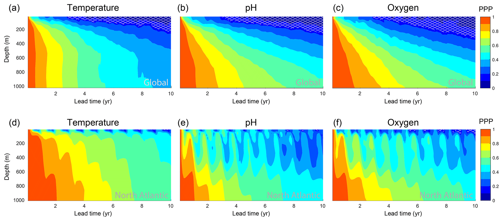
https://www.biogeosciences.net/17/2061/2020/bg-17-2061-2020-f05

Figure 5PPP depth profiles for the top 1000 m for ocean temperature, oxygen and pH at the (a–c) global scale and (d–f) in the North Atlantic. The PPP is shown as monthly means. The light gray hatching indicates a PPP value below the predictability threshold. The North Atlantic is defined as the ocean area between 40 and 60^∘ N in the North Atlantic. Note that the variance over the control simulation for pH is zero for approximately 0.4 % of grid cells at subsurface, which leads to an undefined PPP value there (see Eq. 2). Such grid cells have been excluded here.

Download

The global mean picture of Fig. 5a–c obscures some interesting seasonal features at the regional scale, which are highlighted in Fig. 5d–f for the North Atlantic. Even though the North Atlantic is among the regions with the largest potential predictability at the ocean surface, the predictability at 1000 m depth for pH and O₂ is smaller in the North Atlantic than the global average at the same depth (Fig. 5d–f), especially in boreal winter. For example, the PPP in winter of year 3 for pH is 0.6 at the global scale at 400 m depth (Fig. 5b) but only 0.3 in the North Atlantic (Fig. 5e). The strong connection in the Atlantic between the ocean surface and the upper 1000 m in winter increases the predictability but at the same time decreases the potential predictability within the subsurface. Interestingly, this effect is also visible for temperature but confined to the upper few hundred meters. The reason is that anomalies from the ocean surface do not penetrate as deep for pH and O₂ as they do for temperature.

https://www.biogeosciences.net/17/2061/2020/bg-17-2061-2020-f06

Figure 6Spatial pattern of the predictability time horizon at (a–c) 300 m and (d–f) 1000 m depth for (a, d) ocean temperature, (b, e) pH and (c, f) dissolved oxygen.

Figure 6 shows the spatial pattern of the predictability time horizon for ocean temperature, O₂ and pH at 300 m (panels a–c) and 1000 m (panels d–f) depth, respectively. Although the predictability time horizon is close to 10 years below 300 m on global average, there are specific regions with a reduced predictability time horizon. At 300 m, these regions are the tropical Pacific, the Indian Ocean and parts of the Southern Ocean (Fig. 6a–c). In the equatorial Pacific and Indian Ocean averaged over 20^∘ N and 20^∘ S, the predictability is 4 years for temperature and 7 years for O₂ and pH. For temperature and O₂, the predictability time horizon drops to values lower than 5–6 years in the eastern equatorial Atlantic. At 1000 m depth (Fig. 6d), the spatial pattern of temperature predictability time horizon is similar to the one at 300 m. Large parts of the equatorial Pacific and the Indian Ocean still show relatively short predictability time horizons. This is not the case for O₂ and pH, for which the predictability time horizon largely increases at 1000 m depth compared to 300 m depth in the eastern equatorial Pacific and in the Indian Ocean as well as in the Southern Ocean, so that the predictability time horizon of both O₂ and pH is up to 10 years almost everywhere. Only the western equatorial Pacific (for pH) and the central equatorial Pacific (for O₂) are characterized by reduced potential predictability at 1000 m (predictability time horizons lower than 8 years).

3.3 Deconvolution into physical and biogeochemical control processes

The predictability patterns and timescales presented in the previous sections are investigated next for their underlying dynamical and/or biogeochemical controls. For SST, we compare our findings with previous studies that attributed SST predictability to particular processes. In order to understand the dynamical and biogeochemical control processes of O₂, pH and NPP and to quantify their contribution, we apply a Taylor deconvolution method (see Sect. 2.3.2). It is important to note that a large contribution of a particular driver to the potential predictability of O₂, pH and NPP does not imply a long predictability time horizon of that driver. In addition, the contribution of a process depends not only on its potential predictability (captured by the variance terms in Eq. 3) but also on the potential interaction with the other drivers (covariance terms in Eq. 3).

3.3.1 Sea surface temperature

The long predictability time horizon of SST in the North Atlantic between 40 and 70^∘ N (Fig. 3a) is consistent with previous findings (Boer, 2004; Collins et al., 2006; Griffies and Bryan, 1997a; Pohlmann et al., 2004). The SST in the North Atlantic experiences low-frequency variability that is linked to the Atlantic Meridional Overturning Circulation (AMOC; Buckley and Marshall, 2016). In GFDL-ESM2M, the AMOC experiences strong low-frequency variability, consistent with Msadek et al. (2010), and its predictability time horizon is about 9 years (Fig. C1). Similarly, the Southern Ocean surface waters are also strongly connected to the deep ocean (Morrison et al., 2015), and slow subsurface ocean processes there give rise to decadal predictability in SST (Marchi et al., 2019; Zhang et al., 2017). In CM2.1, the peak in the power spectrum of deep convection in the Weddell Sea is simulated to lie between 70 and 120 years (Zhang et al., 2017). In the North Atlantic and the Southern Ocean, the potential predictability is enhanced during the winter period (Fig. 4), as the surface waters are especially well connected with the deep ocean during the cold season. The long SST predictability time horizon in the Arctic Ocean is due to the overall low-frequency variability in SST there, because these waters are permanently covered by sea ice in the preindustrial ESM2M control simulation and cannot exchange heat (and carbon) with the atmosphere. This is not the case around the Antarctic continent, where sea ice almost vanishes during austral summer in ESM2M, allowing the surface ocean to exchange heat and carbon with the atmosphere. Therefore, the influence of high-frequency atmospheric variability is large, which leads to diminished predictability time horizons around Antarctica. Moderate predictability time horizons in SST of about 3 to 5 years are simulated in the tropical oceans associated with the coupled atmosphere–ocean system (Boer, 2004).

3.3.2 Dissolved oxygen

To understand the processes that give rise to the O₂ predictability pattern, we use a Taylor deconvolution method (see Sect. 2.3.2) to further split the O₂ predictability into respective $O_{2}^{sol}$ and AOU contributions. Figures 7 and 8 show the predictability time horizon of O₂ (identical to patterns shown in Figs. 3c and 6c), $O_{2}^{sol}$ , AOU and their covariance (panels a, b, c and d) as well as their percentage contribution to the normalized ensemble variance (panels e, f and g) for the surface (Fig. 7) and 300 m depth (Fig. 8). The percentage contribution is defined as the value of a given variance term (first term on the right-hand side of the equal sign in Eq. 3) or covariance term (second term on the right-hand side in Eq. 3), divided by the sum of all absolute variance and covariance values. By combining the information from panels e, f and g (i.e., percentage contribution to total predictability) with the information from panels a, b, c and d (i.e., predictability time horizon), we can attribute the local predictability of O₂ to $O_{2}^{sol}$ , AOU or the covariance. For example, if both the percentage contribution and the predictability time horizon of a particular variable are high, then the O₂ predictability is high. If the percentage contribution is generally low for a particular variable, then this variable does not contribute to the overall short or long predictability time horizon of O₂.

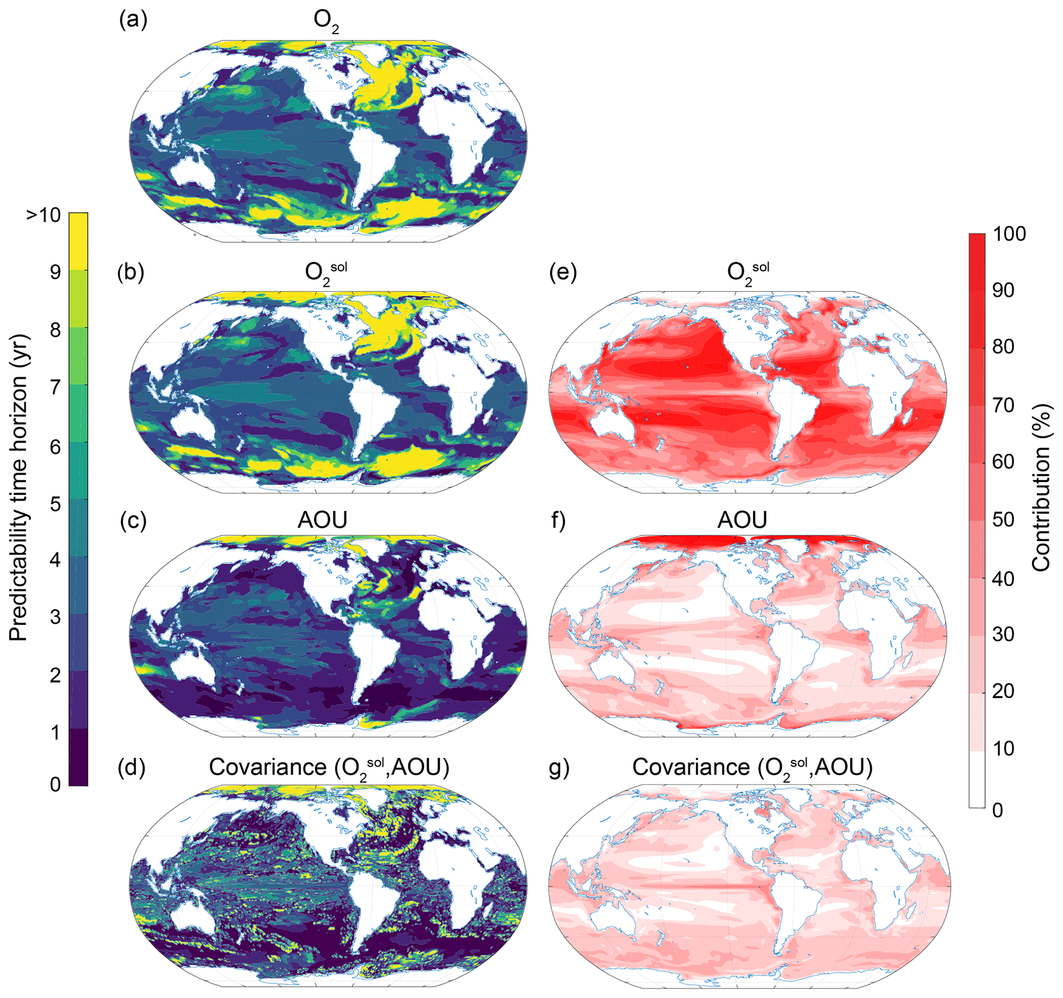
https://www.biogeosciences.net/17/2061/2020/bg-17-2061-2020-f07

Figure 7Spatial pattern of the (a–d) predictability time horizons and (e–g) contribution of different terms to the predictability of oxygen at the surface. (a–d) Predictability time horizon for (a) O₂, (b) $O_{2}^{sol}$ , (c) AOU and (d) covariance between $O_{2}^{sol}$ and AOU. (e–g) Percentage contributions of (e) $O_{2}^{sol}$ , (f) AOU and (g) covariance between $O_{2}^{sol}$ and AOU relative to the sum of all terms. Red shading in panels (e)–(g) represents positive absolute values of the variance and covariance terms. The percentage contributions are shown as averages over the entire 10 years of the simulations. The percentage contributions do not change substantially over the 10 years (always within ±5 % of the 10-year averages).

The largest contribution to the normalized variance in O₂ at the surface stems from $O_{2}^{sol}$ (Fig. 7) with a globally averaged contribution of 58 %, followed by AOU with 23 % and the covariance between $O_{2}^{sol}$ and AOU contributing 19 %. Thus, the $O_{2}^{sol}$ predictability time horizon pattern (Fig. 7b) is almost identical to the O₂ predictability time horizon pattern (Fig. 7a or Fig. 3c), i.e., long predictability time horizons in the North Atlantic, Southern Ocean and Arctic and short predictability time horizons in the midlatitudes. As $O_{2}^{sol}$ at the ocean surface is mainly controlled by temperature (Garcia and Gordon, 1992), it is not surprising that the time horizon pattern of surface O₂ predictability (Figs. 7a and 3c) is also almost identical to the time horizon pattern of SST predictability (Fig. 3a). In the Arctic Ocean and around Antarctica, however, AOU (Fig. 7f) is almost solely responsible for the normalized variance of O₂. As a result, the predictability time horizon of O₂ (Fig. 7a) is similar to the AOU predictability time horizon (Fig. 7c) in these two regions. The covariance between $O_{2}^{sol}$ and AOU overall plays a minor role (Fig. 7g).

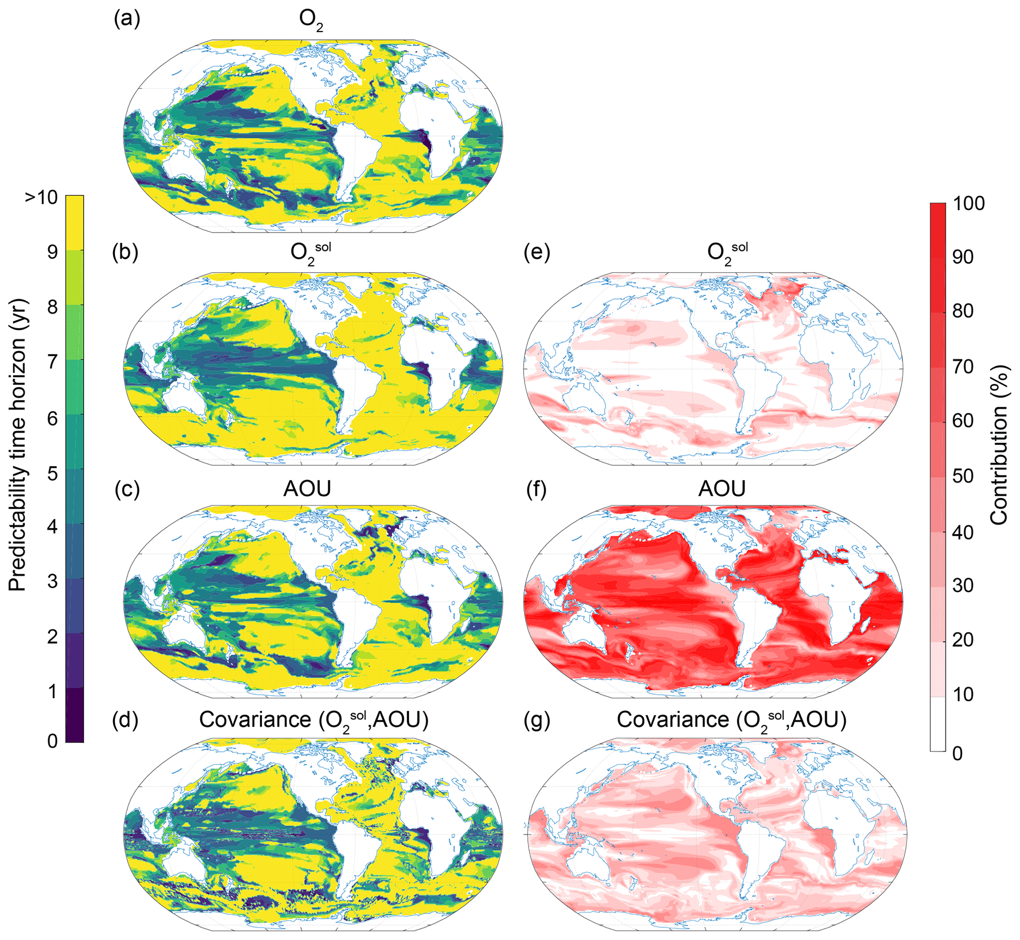
https://www.biogeosciences.net/17/2061/2020/bg-17-2061-2020-f08

Figure 8Same as Fig. 7, but at 300 m depth.

The picture is quite different at 300 m depth (Fig. 8), where the largest contribution percentage-wise to the normalized variance of O₂ stems from AOU (64 % on global average), with minor contributions from $O_{2}^{sol}$ (13 %) and the covariance between $O_{2}^{sol}$ and AOU (23 %). Therefore, the pattern of the AOU predictability time horizon (Fig. 8c) is similar to the pattern of the O₂ predictability time horizon (Fig. 8a). Exceptions are found in the eastern equatorial Pacific, where the covariance dominates (Fig. 8g), and the northern North Atlantic, where $O_{2}^{sol}$ dominates (Fig. 8e). The dominance of AOU in explaining subsurface O₂ predictability is also the reason why O₂ predictability generally increases with depth (Fig. 5c), which is not the case for temperature (Fig. 5a).

3.3.3 pH

The predictability characteristics of pH are decomposed into its primary drivers in the marine carbonate system, namely temperature, salinity, DIC and Alk (Fig. 9). Even though the total normalized ensemble variances from the Taylor deconvolution are only approximations of the total real ensemble variances due to nonlinearities in carbonate chemistry, the values of the Taylor deconvolution are always within ±2 % of the real values, giving us confidence in the appropriateness of the Taylor deconvolution method for pH.

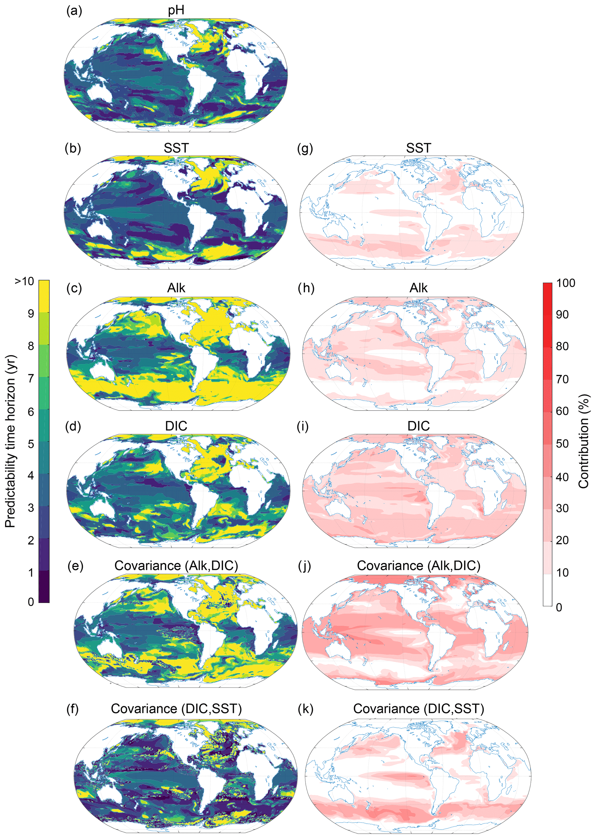
https://www.biogeosciences.net/17/2061/2020/bg-17-2061-2020-f09

Figure 9Spatial pattern of the (a–f) predictability horizons and (g–k) contribution of different terms to the predictability of pH at the surface. (a–f) Predictability time horizon for (a) pH, (b) SST, (c) Alk, (d) DIC, and the covariance between (e) Alk and DIC and (f) DIC and SST. (g–k) Percentage contributions of (g) SST, (h) Alk, (i) DIC, and covariance of (j) ALK and DIC and (k) DIC and SST relative to the sum of all terms. Red shading in panels (g)–(k) represents positive absolute values of the variance and covariance terms. The percentage contributions are shown as averages over the entire 10 years of the simulations. The percentage contributions do not change substantially over the 10 years (always within ±5 % of the 10-year averages). Note that the terms that do not contribute to pH predictability such as sea surface salinity and the covariances between sea surface salinity and all other terms as well as the covariance between SST and Alk are not shown here.

At the surface, the largest contribution percentage-wise stems from the covariance between Alk and DIC (Fig. 9j; with 26 % globally averaged), followed by DIC (Fig. 9i; 22 %), Alk (Fig. 9h; 15 %), the covariance between SST and DIC (Fig. 9k; 14 %), and SST (Fig. 9g; 9 %). All other possible contributors such as sea surface salinity and its covariances (including the covariance between SST and Alk) are not discussed further, as their contributions are below 5 %. The pH predictability time horizon at the surface is mainly determined by Alk and DIC and to a lesser extent SST. The long predictability time horizon of pH in the North Atlantic, the Arctic Ocean and the eastern North Pacific and the short predictability time horizon in the tropical regions (Figs. 9a and 3c) are mainly determined by DIC and Alk and the covariance between DIC and ALK. SST plays a role for parts of the North Atlantic. The predictability of pH in the Southern Ocean is mainly determined by DIC, SST and their covariance. Even though SST exhibits enhanced predictability in the Southern Ocean in relation to pH, the short predictability time horizon of DIC and the covariance of DIC and SST lead to the overall diminished predictability time horizon for pH relative to SST there.

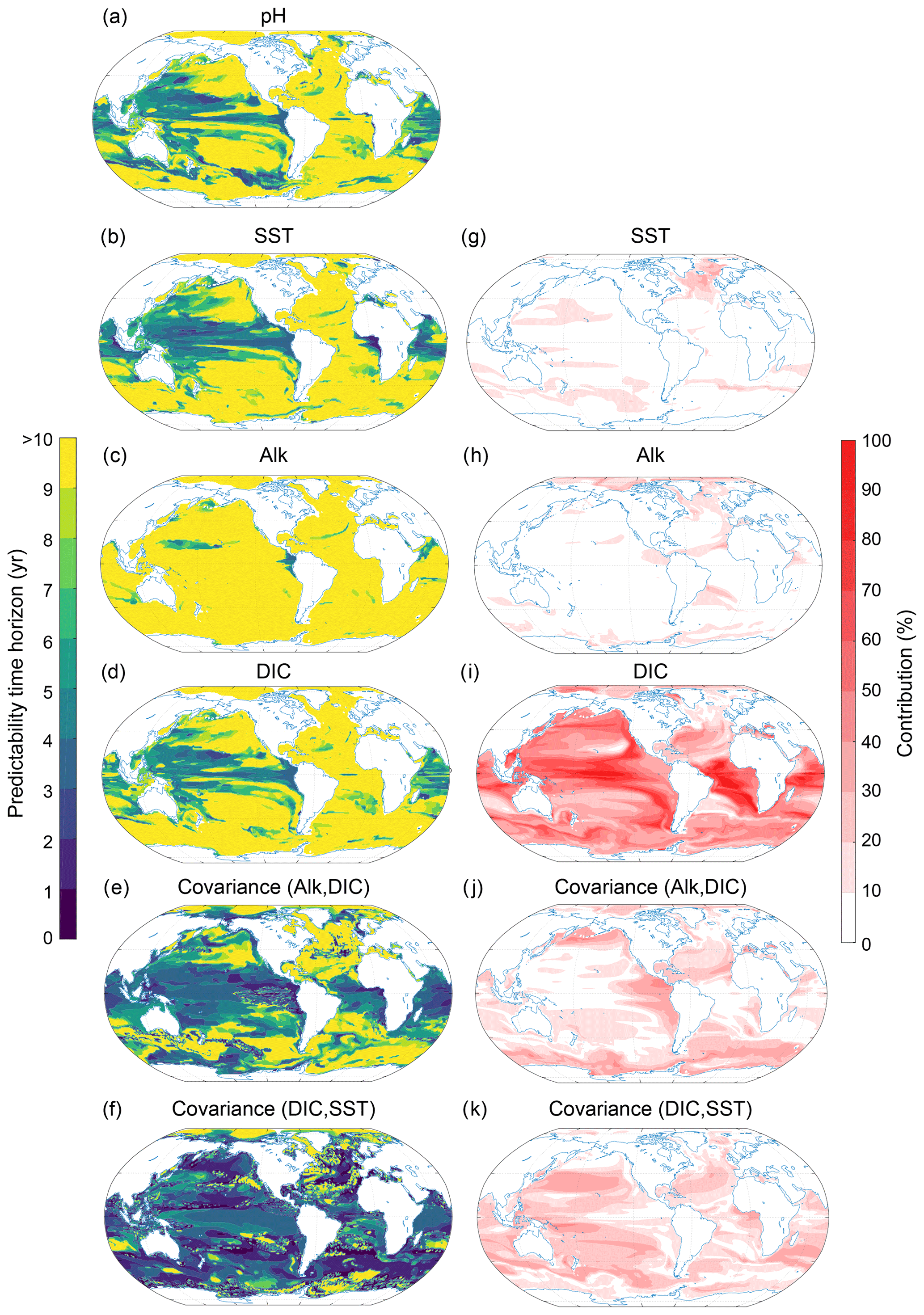
https://www.biogeosciences.net/17/2061/2020/bg-17-2061-2020-f10

Figure 10Same as Fig. 9, but at 300 m depth.

The pH predictability time horizon at 300 m depth (Fig. 10a) is mainly determined by DIC (accounts for 44 % on a global scale; Fig. 10j) and to a lesser extent by the covariance between DIC and SST (19 %; Fig. 10k) and the covariance between Alk and DIC (15 %; Fig. 10j). Interestingly, the relatively short pH predictability time horizon of about 5 years in the western equatorial Pacific and the northern Indian Ocean is also mainly determined by DIC (Fig. 10d, i) and the covariance between DIC and SST (Fig. 10f, k). The short predictability time horizon of pH in the South Pacific is caused by the covariance between SST and DIC. Again, salinity plays a negligible role (not shown).

3.3.4 Net primary production

To understand the drivers that may set the upper limits of NPP predictability, we first split the NPP into the contributions from small-phytoplankton production (NPP_Sm), large-phytoplankton production (NPP_Lg) and production by diazotrophs (NPP_Di; see Sect. 2.3.2 and Appendix A). The largest contribution (i.e., the most important driver of NPP potential predictability) stems from NPP_Sm (65 % averaged globally; Fig. 11). The second most important contributor is the covariance between NPP_Sm and NPP_Lg (19 %) followed by NPP_Lg (9 %). Diazotrophs and all other covariances have only a small impact on the predictability of NPP (less than 5 %; not shown in Fig. 11). The large dominance of NPP_Sm is not unexpected as the small-phytoplankton production overall dominates the total phytoplankton production in ESM2M (Dunne et al., 2013; Laufkötter et al., 2015). NPP_Sm accounts for 84 % of the total NPP at global scales, whereas NPP_Lg and NPP_Di only account for 14 % and 2 %, respectively.

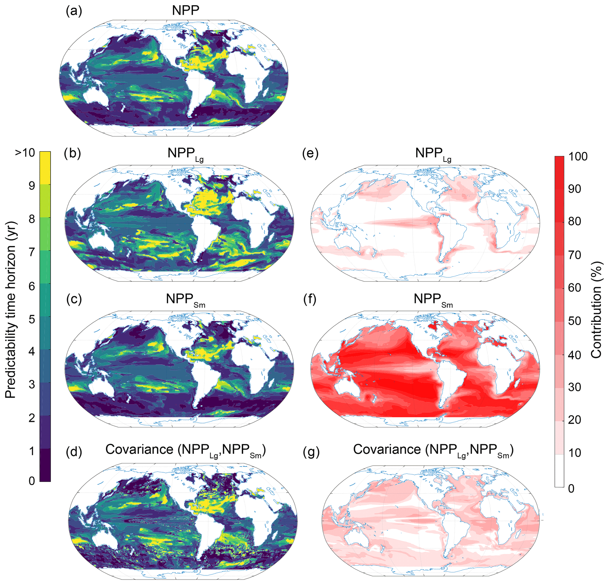
https://www.biogeosciences.net/17/2061/2020/bg-17-2061-2020-f11

Figure 11Spatial pattern of the (a–d) predictability horizons and (e–g) contribution of different terms to the predictability of NPP integrated over the top 100 m. (a–d) Predictability time horizon for (a) NPP, (b) large-phytoplankton production NPP_Lg, (c) small-phytoplankton production NPP_Sm, and (d) the covariance between NPP_Lg and NPP_Sm. (e–g) Percentage contributions of (e) NPP_Lg, (f) NPP_Sm, and (g) covariance of NPP_Lg and NPP_Sm relative to the sum of all terms. Red shading in panels (e)–(g) represents positive absolute values of the variance and covariance terms. The percentage contributions are shown as averages over the entire 10 years of the simulations. The percentage contributions do not change substantially over the 10 years (always within ±5 % of the 10-year averages). Note that the terms that do not substantially contribute to NPP predictability such diazotrophs (NPP_Di) and the covariances between NPP_Di and all other terms are not shown here.

On regional scales, NPP_Smdetermines the predictability of NPP almost everywhere (Fig. 11f). Exceptions are the eastern equatorial Pacific and the higher northern latitudes, where NPP_Lg (Fig. 11e) and the covariance between NPP_Lg and NPP_Sm (Fig. 11g) also play a substantial role. Interestingly, the NPP_Lg (Fig. 11b) has overall a longer predictability time horizon than NPP (Fig. 11a) and NPP_Sm (Fig. 11c).

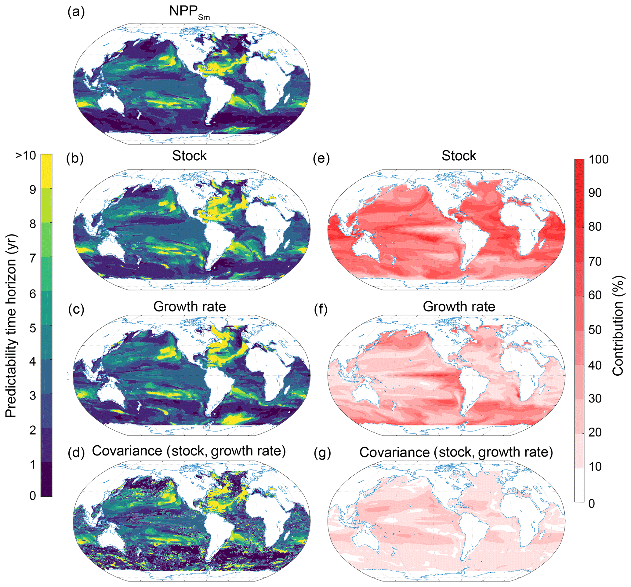
https://www.biogeosciences.net/17/2061/2020/bg-17-2061-2020-f12

Figure 12Spatial pattern of the (a–d) predictability horizons and (e–g) contribution of different terms to the predictability of small-phytoplankton production (NPP_Sm) integrated over the top 100 m. (a–d) Predictability time horizon for (a) NPP_Sm, (b) small-phytoplankton stock, (c) growth rate of small phytoplankton, and (d) the covariance between the stock and the growth rate of small phytoplankton. (e–g) Percentage contributions of (e) stock, (f) growth rate, and (g) covariance of stock and growth rate relative to the sum of all terms. Red shading in panels (e)–(g) represents positive absolute values of the variance and covariance terms. The percentage contributions are shown as averages over the entire 10 years of the simulations. The percentage contributions do not change substantially over the 10 years (always within ±5 % of the 10-year averages).

To understand the drivers of small-phytoplankton predictability, we further deconvolve NPP_Sm into growth rate and small-phytoplankton stock (Fig. 12; Eq. 6 in Sect. 2.3.2). The deconvolution suggests that the largest contribution to the potential predictability on a global scale stems from the small-phytoplankton stock (51 %) followed by the growth rate (31 %) and the covariance between stock and growth rate (18 %). Between 40^∘ S and 40^∘ N, the NPP_Sm predictability is almost solely determined by the small-phytoplankton stock, with the exception of the eastern equatorial Pacific, where the growth rate is more important. Also, the short NPP_Sm predictability time horizon in the North Atlantic mainly originates from the variance of the stock, indicated by the short predictability time horizons of the stock compared to the growth rate there. As we stated previously, NPP has a relatively short potential predictability time horizon over the Southern Ocean compared to the other ecosystem drivers (Fig. 3d). Our analysis shows that small phytoplankton (Fig. 11) and especially the growth rate of the small phytoplankton (Fig. 12) are important for setting this local minimum.

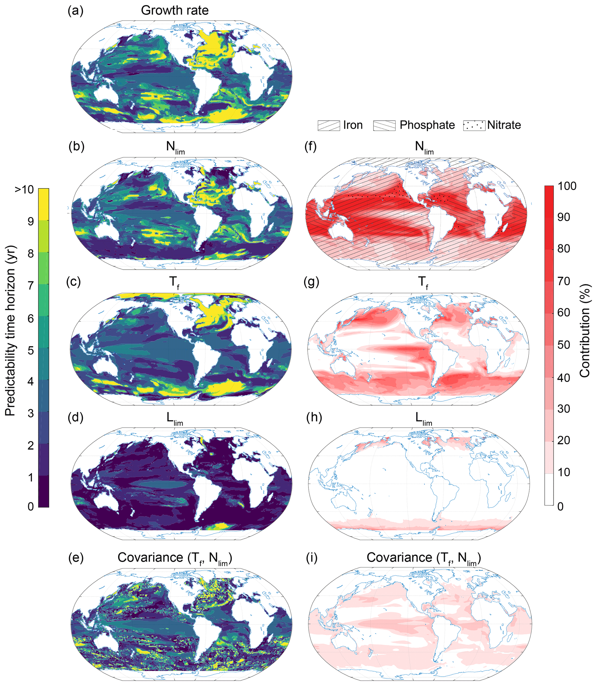
https://www.biogeosciences.net/17/2061/2020/bg-17-2061-2020-f13

Figure 13Spatial pattern of the (a–e) predictability horizons and (f–i) contribution of different terms to the predictability of the small-phytoplankton growth at the surface. (a–e) Predictability time horizon for (a) growth rate of small phytoplankton, (b) nutrient limitation, (c) temperature limitation, (d) light limitation, and (e) the covariance between the temperature and nutrient limitation. (f–i) Percentage contributions of (f) nutrient limitation, (g) temperature limitation, (h) light limitation, and (i) covariance between temperature and nutrient limitation relative to the sum of all terms. Red shading in panels (f)–(i) represents positive absolute values of the variance and covariance terms. The percentage contributions are shown as averages over the entire 10 years of the simulations. The percentage contributions do not change substantially over the 10 years (always within ±5 % of the 10-year averages). Note that the terms that do not substantially contribute to NPP predictability covariances between temperature and light and nutrients are not shown here. The hatching in panel (f) indicates the limiting nutrients as obtained from the 300-year-long preindustrial control simulation.

We further deconvolute the drivers of the surface growth rate predictability of small phytoplankton into their temperature, nutrient and light limiting factors (see Eq. 7 in Sect. 2.3.2; Fig. 13). As the limiting factors are not saved routinely as three-dimensional fields, we focus here on the growth rate and its limiting factors at the surface. Note that the growth rate predictability time horizon at the surface (Fig. 13a) may differ from the growth rate predictability time horizon integrated over the top 100 m (Fig. 12c), especially in the Southern Ocean and the North Atlantic. At the surface and at the global scale, the largest contribution stems from the nutrient limitation term (50 %) followed by the temperature limitation term (25 %) and the covariance between the temperature and nutrient limitations (13 %). At the regional scale, the nutrient limitation term clearly dominates at midlatitudes (Fig. 13f). In GFDL-ESM2M, the subtropical gyres are mainly iron limited (hatching in Fig. 13f), and therefore iron fundamentally constrains the predictability of the growth rate of small phytoplankton there. Exceptions are the boundary region between the subtropical and subpolar gyre in the North Pacific (nitrate limited) as well as the tropical Atlantic (phosphate and nitrate) and the northern Indian Ocean (phosphate). GFDL-ESM2M's overall strong iron limitation is in contrast to the findings of Moore et al. (2013), who suggest that nitrogen is the limiting nutrient in the subtropical gyres. GFDL-ESM2M is a fully coupled Earth system model and assesses iron limitation through the ability to synthesize chlorophyll. In contrast, Moore et al. (2013) use observation-driven parameterizations of phytoplankton growth and assess iron limitation through nutrient uptake alone. The temperature limitation term is dominant in the higher latitudes and the eastern equatorial Pacific (Fig. 13g). The light limitation term only plays a substantial role (up to 20 %) around Antarctica and close to the Arctic sea ice edge (Fig. 13h). The simulated long predictability time horizon for NPP in the midlatitudes can therefore be attributed to the long predictability time horizon of the nutrient limitation, especially given that the growth rate predictability at the surface is similar to the growth rate predictability integrated over the top 100 m in this region. At latitudes north of 40^∘ N and south of 40^∘ S, the temperature limitation is the most important contributor. Therefore, the predictability time horizon pattern of the growth rate strongly resembles the one for SST in these regions. In the Southern Ocean, however, the growth rate predictability time horizon at the surface is much longer than the growth rate predictability integrated over the top 100 m, indicating that a process other than temperature (e.g., light limitation) may limit predictability there.

4 Discussion and conclusion

We set out three goals for this study: (a) assessing the global characteristics of potential predictability for temperature, pH, O₂ and NPP, as a mean to identify an upper bound on our ability to predict conditions for marine ecosystems; (b) assessing regional and depth-dependent characteristics of potential predictability; and (c) identifying the potential mechanisms that limit or increase predictability for the different marine ecosystem drivers. This was pursued within a perfect modeling framework using a comprehensive Earth system model.

The analysis revealed that on global scales the predictability time horizon of each variable is surprisingly similar, i.e., 3 years for all four marine ecosystem drivers (Fig. 2; first goal), despite the fact that the regional processes operating are different over a range of scales (second and third goal). This is unexpected, as the ocean processes that sustain the disparate divers should not be expected to have identical memory as pertains to predictability. For example the relatively long predictability time horizon identified for SST and surface O₂ over the subpolar North Atlantic (the SST to be consistent with Griffies and Bryan, 1997a, b; Boer, 2000; Collins et al., 2006; Keenlyside et al., 2008) and the Southern Ocean (consistent with Zhang et al., 2017 and Marchi et al., 2019) is not reflected in NPP. Likewise, the long predictability time horizon of NPP in the subtropical gyres is not simulated for other ecosystem drivers, and the short predictability time horizon of surface pH in the Southern Ocean is reflected in neither SST nor surface O₂.

Our results suggesting the same global predictability time horizon for all four ecosystem drivers are not inconsistent with time of emergence diagnostics for transient climate warming scenarios where pH (early emergence) and NPP (late emergence) behave oppositely (Frölicher et al., 2016; Rodgers et al., 2015; Schlunegger et al., 2019). Time of emergence is defined as the ratio (large for pH and small for NPP) of the anthropogenic forced change to the background internal variability. Comparing our results with the time of emergence analysis is therefore complicated by the presence of the anthropogenic forced signal in scenario projections. In fact it is the presence of the large invasion flux for CO₂ that renders acidification the most rapidly emergent of the drivers under anthropogenic perturbations, in particular relative to NPP. The similarities between the analyses of predictability and emergence timescales lie in the noise, which is expected to include not only modes of climate variability such as El Niño–Southern Oscillation (ENSO) but also higher-frequency variability such as cloud cover that may impact NPP for both cases.

Our study complements earlier studies which suggested that marine ecosystem drivers may be predictable on multi-annual timescales. In contrast to earlier studies (Chikamoto et al., 2015; Park et al., 2019; Séférian et al., 2014b), rather than focusing on a single ecosystem driver, we compare and contrast the potential predictability of four marine ecosystem drivers and also evaluate the processes behind their respective predictability limits. We find that in contrast to SST, these ecosystem drivers depend on a complex interplay between physical and biogeochemical underlying processes. For O₂, the importance of subsurface AOU reveals a complex interplay between nonlocal circulation and biological consumption, whereas at the surface O₂ is mainly determined by the predictability of SST. For NPP, the growth rate of the small phytoplankton in the Southern Ocean is important for setting the local minimum in predictability time horizon there. The predictability time horizon of surface pH is mainly determined by a complex interplay between DIC and Alk predictability in the low latitudes and DIC, Alk and temperature predictability in high latitudes. Interestingly, we find longer predictability time horizons for SST than for NPP in the equatorial Pacific, which is in contrast to findings of Séférian et al. (2014a). Importantly, this may be indicative of a potential model dependency of the relationship between ecosystem driver predictability. Séférian et al. (2014b) attributed longer NPP predictability time horizons to the idea that the nutrient supply processes that modulate NPP are themselves regulated by thermocline wave adjustment processes, without sizable modulation by surface fluxes. This was framed as being in contrast to the case of SST, where air–sea fluxes reflecting higher-frequency variations act to reduce the predictability of SST. In ESM2M, the predictability time horizon for SST in the eastern equatorial Pacific (biome 6 in Fig. 4) is approximately 3.5 years, modestly longer than the predictability time horizon for NPP of approximately 3 years. In ESM2M, NPP is only weakly correlated with changes in upwelling and nutrient supply in the eastern tropical Pacific (as was shown in Fig. 2 of Kwiatkowski et al., 2017). This is confirmed by our analysis showing that nutrient limitation is not the dominant term for explaining the predictability of NPP there. This indicates that less predictable processes occurring over shorter timescales, such as temperature and/or light level variations, influence NPP predictability.

Even though we consider our conclusion to be robust, a number of potential caveats warrant discussion. These include the (i) ensemble design of the perfect model simulations (e.g., initialization and number of ensemble members) and (ii) the impact of model formulation and biases. For the first of these caveats, our simulations are all initialized with SST perturbations applied to a single grid cell in the Weddell Sea, and therefore a different spatial perturbation strategy may give different results. However, as the signal at the ocean surface spreads very rapidly (i.e., after 4 d all grid cells at the ocean surface are perturbed) our results are insensitive to the spatial initialization method, at least in the upper ocean. Second, all ensemble simulations start on 1 January of the corresponding simulation year. It has been shown that the forecast skill of seasonal predictions may depend strongly on the way the models are initialized. ENSO forecasts, for example, have a much lower predictability if they are initialized before and through spring (Webster and Yang, 1992). However, as our focus is on annual to decadal timescales, this effect is less important for our analysis. Third, we have employed only six starting points for our 40-member ensemble simulation. Even though all six ensemble simulations branched off at different El Niño–Southern Oscillation states of the preindustrial control simulation, our choice of six macro-perturbations may still introduce aliasing issues that could bias our results. Although the computing resources at our disposal for this study did not allow for expanding the number of starting points, we recommend that future studies with CMIP-class models should expand the number of initialization points to further explore the sensitivity of the results to the starting point of the ensembles.

The second caveat in our study is that we only used one single Earth system model and that our results might depend on the model formulation and resolution. Even though the GFDL-ESM2M model achieves sufficient fidelity in its preindustrial states (Bopp et al., 2013; Dunne et al., 2012, 2013; Laufkötter et al., 2015), it is well known that CMIP5-generation models have imperfect representation of biogeochemical and physical processes as well as variability over a range of timescales, ranging from weather variability to ENSO variability (Frölicher et al., 2016; Resplandy et al., 2015) to decadal variability (England et al., 2014; McGregor et al., 2014). Different physical and biogeochemical parameterizations within a given model may change the length of the predictability time horizon. For example, TOPAZ2 represents a hypothetically optimal phytoplankton physiology; namely the model assumes that the fastest growing phytoplankton group always wins in all environments via the upper limit in growth rates. In addition, TOPAZv2 represents a steady-state ecosystem, such that there are no time lags between primary production and the grazing response. In the subsurface, the remineralization of particles is set to reproduce the vertical scale of the nutricline on the timescale of sinking particles, and the sinking particle velocity is fast. All three factors may tend to decrease the memory associated with the real-world surface ecosystem and minimize predictability. For the case of weather prediction, it has been argued that the inclusion of stochastic parameterizations increases potential predictability (Palmer and Williams, 2008). To our knowledge, this remains unexplored for marine biogeochemistry and ecosystem drivers. In any case, it would be necessary to repeat our predictability experiments with a set of different Earth system models including different parameterizations of biogeochemical and/or physical ocean processes to investigate the dependence of our result on the model representation (Séférian et al., 2018), in parallel with broader efforts to further evaluate noise characteristics of these models. Additionally, the ocean model resolution of GFDL-ESM2M is rather coarse and cannot represent the critical scales of small-scale structures of circulation. Predictability studies using high-resolution ocean models with improved process representations are therefore needed to explore potential predictability, especially at the local scale. However, it is currently impossible in many cases to constrain the simulated variability in biogeochemical drivers, especially for the ocean subsurface, with observations due to limited data availability (Frölicher et al., 2016; Laufkötter et al., 2015).

Currently, no global coupled physical–biogeochemical seasonal to decadal forecast system is yet operational (Tommasi et al., 2017). However, our study suggests great promise that physical–biogeochemical forecast systems may have the potential to provide useful information to a wide group of stakeholders, such as, for example, for the management of fisheries (Dunn et al., 2016; Park et al., 2019). Our study therefore underscores the need to further develop integrated physical–biogeochemical forecast systems. Especially in regions with long predictability time horizons, such as the North Atlantic (for temperature, O₂ and pH), the Southern Ocean (for temperature and O₂) and midlatitudes (for NPP), installing and maintaining a spatially and temporally dense physical and biogeochemical ocean observing system would have the potential to significantly improve the effective predictability of marine ecosystem drivers.

Appendix A

The NPP in TOPAZ2, defined as the phytoplankton nitrogen production, is individually described for all phytoplankton groups i by the product of a phytoplankton growth rate μ_i and the amount of nitrogen in the plankton group [N]_i (see Table A1 for numerical values of parameters used in TOPAZ2):

\begin{matrix} (A1) & {NPP}_{i} = μ_{i} \cdot {[N]}_{i} . \end{matrix}

The growth rate of the small-phytoplankton group is given by a maximum growth rate times the limiting factors of nutrients N_lim, light L_lim and temperature T_f:

\begin{matrix} (A2) & μ_{Sm} = \frac{μ_{max}^{'}}{1 + ζ} \cdot N_{\lim} \cdot L_{\lim} \cdot T_{f} . \end{matrix}

The temperature limitation factor is

\begin{matrix} (A3) & T_{f} = \exp (k_{epp} \cdot T) . \end{matrix}

The nutrient limitation factor is

\begin{matrix} (A4) & N_{\lim} = min (N_{Fe}, N_{{PO}_{4}}, N_{{NO}_{3}} + N_{{NH}_{4}}), \end{matrix}

with iron limitation

\begin{matrix} (A5) & N_{Fe} = \frac{Q_{Fe : N}^{2}}{Q_{Fe : N}^{2} + K_{Fe : N}^{2}} \end{matrix}

with

Q_{Fe : N} = min (Q_{Fe : N_{\max}}, \frac{{[Fe]}_{Sm}}{{[N]}_{Sm}}),

with phosphate limitation

\begin{matrix} (A6) & N_{{PO}_{4}} = \frac{Q_{P : N}}{Q_{P : N_{\max}}} \end{matrix}

with

Q_{P : N} = min (Q_{P : N_{\max}}, \frac{{[P]}_{Sm}}{{[N]}_{Sm}}),

with nitrate limitation

\begin{matrix} (A7) & N_{{NO}_{3}} = \frac{[{NO}_{3}]}{[{NO}_{3}] + K_{{NO}_{3}}} \cdot \frac{1 + [{NH}_{4}]}{K_{{NH}_{4}}}, \end{matrix}

and with ammonium limitation

\begin{matrix} (A8) & N_{{NH}_{4}} = \frac{[{NH}_{4}]}{[{NH}_{4}] + K_{{NH}_{4}}} . \end{matrix}

The light limitation factor is

\begin{matrix} (A9) & L_{\lim} = 1 - \exp (\frac{- α θ [IRR]}{N_{\lim} T_{f} μ_{max}}) \end{matrix}

with

\begin{matrix} (A10) & \begin{aligned} θ & = \frac{θ_{max} - θ_{min}}{1 + (θ_{max} - θ_{min}) α [{IRR}_{mem}] / (2 N_{\lim} T_{f} μ_{max})} \\ + θ_{min} \end{aligned} \end{matrix}

and

\begin{matrix} (A11) & θ_{min} = max (0, θ_{min}^{nolim} - θ_{min}^{\lim}) \cdot N_{\lim} + θ_{min}^{\lim}, \end{matrix}

where [IRR] describes the photosynthetically active radiation and [IRR_mem] is the irradiation memory over the last 24 h.

Table A1TOPAZ2 parameters for small phytoplankton.

Download Print Version | Download XLSX

Appendix B

Potential predictability may depend on the choice of the predictability metric (Hawkins et al., 2016). Therefore, we calculate two additional metrics to assess the robustness of our results: the normalized root-mean-square error (NRMSE) and the intra-ensemble anomaly correlation coefficient (ACC_I). The NRMSE is similar to the PPP but uses standard deviations instead of variances and compares every ensemble member to every other member of that ensemble, thereby increasing the effective sample size (Collins et al., 2006):

\begin{matrix} (B1) & NRMSE (t) = 1 - \sqrt{\frac{{〈{(X_{i j} (t) - X_{k j} (t))}^{2}〉}_{i, j, k \neq i}}{2 σ_{c}^{2}}} . \end{matrix}

〈⋅〉 means that we sum over the listed indices and divide by the degrees of freedom. The intra-ensemble anomaly correlation coefficient (ACC_I) is a measure for the correlation between the anomaly of all ensemble members of an ensemble averaged over all ensembles and is regularly used for assessing operational predictions (Goddard et al., 2013). The anomaly is defined as the deviation of a given value from the climatological mean μ_j (i.e., the mean over the control run) over the jth ensemble period.

\begin{matrix} (B2) & {ACC}_{I} (t) = \frac{{〈(X_{i j} (t) - μ_{j}) (X_{k j} (t) - μ_{j})〉}_{i, j, k \neq i}}{{〈{(X_{i j} (t) - μ_{j})}^{2}〉}_{i, j}} \end{matrix}

While PPP and NRMSE estimate predictability by comparing the spread of the ensembles to the natural variability from the control simulation, the anomaly correlation coefficients include the phase alignment of the ensembles and the control simulation. We again use a F test for NRMSE and a t test for ACC_I to estimate the predictability threshold.

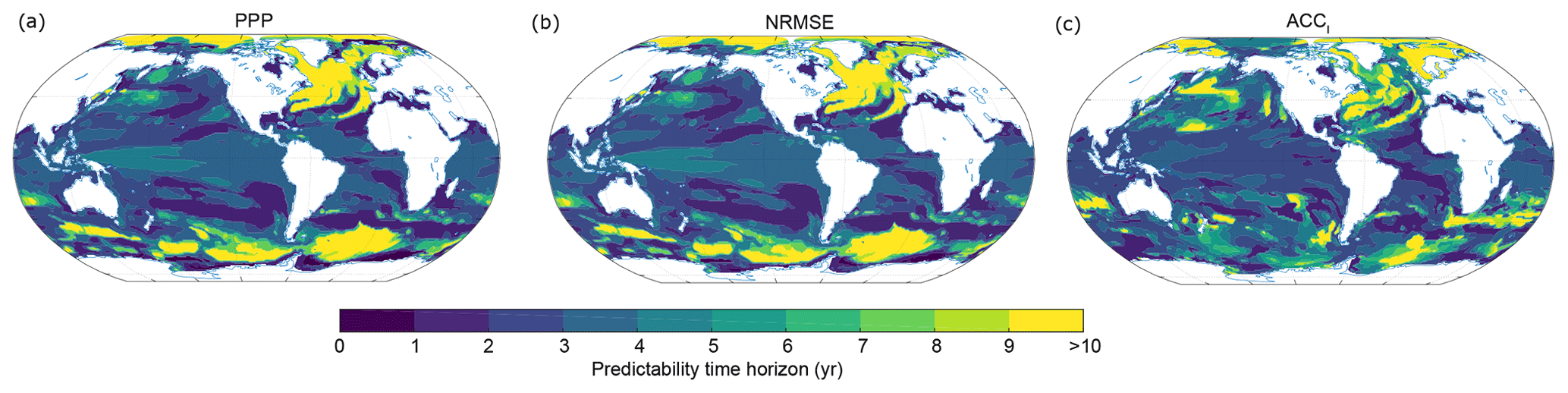
https://www.biogeosciences.net/17/2061/2020/bg-17-2061-2020-f14

Figure B1SST predictability time horizon calculated with different metrics. Spatial pattern of the predictability horizon for sea surface temperature using (a) PPP, (b) NRMSE and (c) ACC_I. Note that we assume an arbitrary predictability threshold for ACC_I so that the emerging pattern matches the PPP predictability best. This allows us to compare the relative differences in predictability.

Figure B1 compares the two additional metrics applied to SST with the PPP metric. We introduce an artificial predictability threshold for ACC_I in such a way that the emerging pattern matches the predictability time horizon best. This allows us to compare the relative differences in predictability between the metrics best. The predictability pattern for SST obtained from all three metrics is very similar. In particular the patterns obtained using PPP and NRMSE are nearly identical. This can be expected since both the PPP and the NRMSE estimate potential predictability by analyzing the ensemble spread. The ACC_I shows some small differences from PPP and NRMSE, especially in the Southern Ocean and the North Pacific.

Appendix C

https://www.biogeosciences.net/17/2061/2020/bg-17-2061-2020-f15

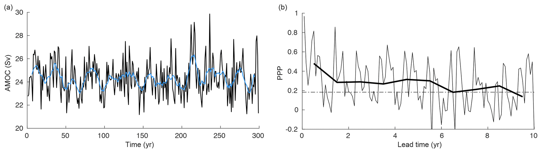
Figure C1(a) Simulated annual mean AMOC maximum of the 300-year-long preindustrial control simulation. The blue line indicates the 10-year running mean. (b) Monthly mean (thin line) and annual mean (thick line) prognostic potential predictability for the AMOC maximum. The horizontal black dashed line represents the predictability threshold.

Download

Data availability

The GFDL-ESM2M simulations are available upon request.

Author contributions

TLF, KBR, LR and CCR designed the study. TLF set up the ensemble simulations and KBR performed the simulations. JD is the lead developer of TOPAZ2. LR performed most of the analysis. TLF wrote the initial manuscript. All authors contributed significantly to the writing of the paper.

Competing interests

The authors declare that they have no conflict of interest.

Acknowledgements

Thomas L. Frölicher and Luca Ramseyer acknowledge support from the Swiss National Supercomputing Centre (CSCS). The authors thank Friedrich Burger for discussions on the Taylor deconvolution method and Natacha Le Grix for discussion on the TOPAZ2 model code.

Financial support

This research has been supported by the Swiss National Science Foundation (grant no. PP00P2_170687), the EU H2020 (grant no. 821003) and the Institute for Basic Science (grant no. IBS-R028-D1).

Review statement

This paper was edited by Stefano Ciavatta and reviewed by Mark Baird and one anonymous referee.

References

Anderson, J. L., Balaji, V., Broccoli, A. J., Cooke, W. F., Delworth, T. L., Dixon, K. W., Donner, L. J., Dunne, K. A., Freidenreich, S. M., Garner, S. T., Gudgel, R. G., Gordon, C. T., Held, I. M., Hemler, R. S., Horowitz, L. W., Klein, S. A., Knutson, T. R., Kushner, P. J., Langenhost, A. R., Lau, N. C., Liang, Z., Malyshev, S. L., Milly, P. C. D., Nath, M. J., Ploshay, J. J., Ramaswamy, V., Schwarzkopf, M. D., Shevliakova, E., Sirutis, J. J., Soden, B. J., Stern, W. F., Thompson, L. A., Wilson, R. J., Wittenberg, A. T., and Wyman, B. L.: The new GFDL global atmosphere and land model AM2-LM2: Evaluation with prescribed SST simulations, J. Climate, 17, 4641–4673, https://doi.org/10.1175/JCLI-3223.1, 2004.

Boer, G. J.: A study of atmosphere-ocean predictability on long time scales, Clim. Dynam., 16, 469–477, https://doi.org/10.1007/s003820050340, 2000.

Boer, G. J.: Long time-scale potential predictability in an ensemble of coupled climate models, Clim. Dynam., 23, 29–44, https://doi.org/10.1007/s00382-004-0419-8, 2004.

Bopp, L., Resplandy, L., Orr, J. C., Doney, S. C., Dunne, J. P., Gehlen, M., Halloran, P., Heinze, C., Ilyina, T., Séférian, R., Tjiputra, J., and Vichi, M.: Multiple stressors of ocean ecosystems in the 21st century: projections with CMIP5 models, Biogeosciences, 10, 6225–6245, https://doi.org/10.5194/bg-10-6225-2013, 2013.

Buckley, M. W. and Marshall, J.: Observations, inferences, and mechanisms of the Atlantic Meridional Overturning Circulation: A review, Rev. Geophys., 54, 5–63, https://doi.org/10.1002/2015RG000493, 2016.

Chikamoto, O. M., Timmermann, A., Chikamoto, Y., Tokinaga, H., and Harada, N.: Mechanisms and predictability of multiyear ecosystem variability in the North Pacific, Global Biogeochem. Cy., 29, 2001–2019, https://doi.org/10.1002/2015GB005096, 2015.

Collins, M., Botzet, M., Carril, A. F., Drange, H., Jouzeau, A., Latif, M., Masina, S., Otteraa, O. H., Pohlmann, H., Sorteberg, A., Sutton, R., and Terray, L.: Interannual to Decadal Climate Predictability in the North Atlantic: A Multimodel-Ensemble Study, J. Climate, 19, 1195–1203, https://doi.org/10.1175/JCLI3654.1, 2006.

Delworth, T. L., Broccoli, A. J., Rosati, A., Stouffer, R. J., Balaji, V., Beesley, J. A., Cooke, W. F., Dixon, K. W., Dunne, J., Dunne, K. A., Durachta, J. W., Findell, K. L., Ginoux, P., Gnanadesikan, A., Gordon, C. T., Griffies, S. M., Gudgel, R., Harrison, M. J., Held, I. M., Hemler, R. S., Horowitz, L. W., Klein, S. A., Knutson, T. R., Kushner, P. J., Langenhorst, A. R., Lee, H. C., Lin, S. J., Lu, J., Malyshev, S. L., Milly, P. C. D., Ramaswamy, V., Russell, J., Schwarzkopf, M. D., Shevliakova, E., Sirutis, J. J., Spelman, M. J., Stern, W. F., Winton, M., Wittenberg, A. T., Wyman, B., Zeng, F., and Zhang, R.: GFDL's CM2 global coupled climate models. Part I: Formulation and simulation characteristics, J. Climate, 19, 643–674, https://doi.org/10.1175/JCLI3629.1, 2006.

Drinkwater, K. F., Beaugrand, G., Kaeriyama, M., Kim, S., Ottersen, G., Perry, R. I., Pörtner, H.-O., Polovina, J. J., and Takasuka, A.: On the processes linking climate to ecosystem changes, J. Marine Syst., 79, 374–388, https://doi.org/10.1016/j.jmarsys.2008.12.014, 2010.

Dunn, D. C., Maxwell, S. M., Boustany, A. M., and Halpin, P. N.: Dynamic ocean management increases the efficiency and efficacy of fisheries management, P. Natl. Acad. Sci. USA, 113, 668–673, https://doi.org/10.1073/pnas.1513626113, 2016.

Dunne, J. P., John, J. G., Adcroft, A. J., Griffies, S. M., Hallberg, R. W., Shevliakova, E., Stouffer, R. J., Cooke, W., Dunne, K. A., Harrison, M. J., Krasting, J. P., Malyshev, S. L., Milly, P. C. D., Phillipps, P. J., Sentman, L. T., Samuels, B. L., Spelman, M. J., Winton, M., Wittenberg, A. T., and Zadeh, N.: GFDL's ESM2 Global Coupled Climate-Carbon Earth System Models. Part I: Physical Formulation and Baseline Simulation Characteristics, J. Climate, 25, 6646–6665, https://doi.org/10.1175/JCLI-D-11-00560.1, 2012.

Dunne, J. P., John, J. G., Shevliakova, S., Stouffer, R. J., Krasting, J. P., Malyshev, S. L., Milly, P. C. D., Sentman, L. T., Adcroft, A. J., Cooke, W., Dunne, K. A., Griffies, S. M., Hallberg, R. W., Harrison, M. J., Levy, H., Wittenberg, A. T., Phillips, P. J., and Zadeh, N.: GFDL's ESM2 global coupled climate-carbon earth system models. Part II: Carbon system formulation and baseline simulation characteristics, J. Climate, 26, 2247–2267, https://doi.org/10.1175/JCLI-D-12-00150.1, 2013.

Eade, R., Hermanson, L., Robinson, N., Smith, D., Hermanson, L., and Robinson, N.: Do seasonal-to-decadal climate predictions underestimate the predictability of the real world?, Geophys. Res. Lett., 41, 5620–5628, https://doi.org/10.1002/2014GL061146, 2014.

England, M. H., McGregor, S., Spence, P., Meehl, G. a, Timmermann, A., Cai, W., Gupta, A. Sen, McPhaden, M. J., Purich, A., and Santoso, A.: Recent intensification of wind-driven circulation in the Pacific and the ongoing warming hiatus, Nat. Clim. Change, 4, 222–227, https://doi.org/10.1038/NCLIMATE2106, 2014.

Fay, A. R. and McKinley, G. A.: Global open-ocean biomes: mean and temporal variability, Earth Syst. Sci. Data, 6, 273–284, https://doi.org/10.5194/essd-6-273-2014, 2014.

Frölicher, T. L., Joos, F., Plattner, G. K., Steinacher, M., and Doney, S. C.: Natural variability and anthropogenic trends in oceanic oxygen in a coupled carbon cycle-climate model ensemble, Global Biogeochem. Cy., 23, GB1003, https://doi.org/10.1029/2008GB003316, 2009.

Frölicher, T. L., Rodgers, K. B., Stock, C. A., and Cheung, W. W. L.: Sources of uncertainties in 21st century projections of potential ocean ecosystem stressors, Global Biogeochem. Cy., 30, 1224–1243, https://doi.org/10.1002/2015GB005338, 2016.

Garcia, H. E. and Gordon, L. I.: Oxygen solubility in seawater: Better fitting equations, Limnol. Oceanogr., 37, 1307–1312, https://doi.org/10.4319/lo.1992.37.6.1307, 1992.

Gattuso, J.-P., Magnan, A., Bille, R., Cheung, W. W. L., Howes, E. L., Joos, F., Allemand, D., Bopp, L., Cooley, S. R., Eakin, C. M., Hoegh-Guldberg, O., Kelly, R. P., Portner, H.-O., Rogers, A. D., Baxter, J. M., Laffoley, D., Osborn, D., Rankovic, A., Rochette, J., Sumaila, U. R., Treyer, S., and Turley, C.: Contrasting futures for ocean and society from different anthropogenic CO₂ emissions scenarios, Science, 349, 1–10, 2015.

Gehlen, M., Barciela, R., Bertino, L., Brasseur, P., Butenschön, M., Chai, F., Crise, A., Drillet, Y., Ford, D., Lavoie, D., Lehodey, P., Perruche, C., Samuelsen, A., and Simon, E.: Building the capacity for forecasting marine biogeochemistry and ecosystems: recent advances and future developments, J. Oper. Oceanogr., 8, s168–s187, https://doi.org/10.1080/1755876X.2015.1022350, 2015.

Gnanadesikan, A., Dunne, J. P., and John, J.: Understanding why the volume of suboxic waters does not increase over centuries of global warming in an Earth System Model, Biogeosciences, 9, 1159–1172, https://doi.org/10.5194/bg-9-1159-2012, 2012.

Goddard, L., Kumar, A., Solomon, A., Smith, D., Boer, G., Gonzalez, P., Kharin, V., Merryfield, W., Deser, C., Mason, S. J., Kirtman, B. P., Msadek, R., Sutton, R., Hawkins, E., Fricker, T., Hegerl, G., Ferro, C. A. T., Stephenson, D. B., Meehl, G. A., Stockdale, T., Burgman, R., Greene, A. M., Kushnir, Y., Newman, M., Carton, J., Fukumori, I., and Delworth, T.: A verification framework for interannual-to-decadal predictions experiments, Clim. Dynam., 40, 245–272, https://doi.org/10.1007/s00382-012-1481-2, 2013.

Griffies, S. M.: Elements of the Modular Ocean Model (MOM), GFDL Model Doc., 3, 1–631, 2012.

Griffies, S. M. and Bryan, K.: A predictability study of simulated North Atlantic multidecadal variability, Clim. Dynam., 13, 459–487, https://doi.org/10.1007/s003820050177, 1997a.

Griffies, S. M. and Bryan, K.: Predictability of North Atlantic Multidecadal Climate Variability, Science, 275, 181–184, https://doi.org/10.1126/science.275.5297.181, 1997b.

Gruber, N.: Warming up, turning sour, losing breath: ocean biogeochemistry under global change, Philos. T. Roy. Soc. A, 369, 1980–1996, https://doi.org/10.1098/rsta.2011.0003, 2011.

Hawkins, E., Tietsche, S., Day, J. J., Melia, N., Haines, K., and Keeley, S.: Aspects of designing and evaluating seasonal-to-interannual Arctic sea-ice prediction systems, Q. J. Roy. Meteor. Soc., 142, 672–683, https://doi.org/10.1002/qj.2643, 2016.

Hobday, A. J., Spillman, C. M., Paige Eveson, J., and Hartog, J. R.: Seasonal forecasting for decision support in marine fisheries and aquaculture, Fish. Oceanogr., 25, 45–56, https://doi.org/10.1111/fog.12083, 2016.

Keenlyside, N. S., Latif, M., Jungclaus, J., Kornblueh, L., and Roeckner, E.: Advancing decadal-scale climate prediction in the North Atlantic sector, Nature, 453, 84–88, https://doi.org/10.1038/nature06921, 2008.

Kumar, A., Peng, P., and Chen, M.: Is There a Relationship between Potential and Actual Skill?, Mon. Weather Rev., 142, 2220–2227, https://doi.org/10.1175/MWR-D-13-00287.1, 2014.

Kwiatkowski, L., Bopp, L., Aumont, O., Ciais, P., Cox, P. M., Laufkötter, C., Li, Y., and Séférian, R.: Emergent constraints on projections of declining primary production in the tropical oceans, Nat. Clim. Chang., 7, 355–358, https://doi.org/10.1038/nclimate3265, 2017.

Laufkötter, C., Vogt, M., Gruber, N., Aita-Noguchi, M., Aumont, O., Bopp, L., Buitenhuis, E., Doney, S. C., Dunne, J., Hashioka, T., Hauck, J., Hirata, T., John, J., Le Quéré, C., Lima, I. D., Nakano, H., Seferian, R., Totterdell, I., Vichi, M., and Völker, C.: Drivers and uncertainties of future global marine primary production in marine ecosystem models, Biogeosciences, 12, 6955–6984, https://doi.org/10.5194/bg-12-6955-2015, 2015.

Lehodey, P., Alheit, J., Barange, M., Baumgartner, T., Beaugrand, G., Drinkwater, K., Fromentin, J.-M., Hare, S. R., Ottersen, G., Perry, R. I., Roy, C., van der Lingen, C. D., and Werner, F.: Climate Variability, Fish, and Fisheries, J. Climate, 19, 5009–5030, https://doi.org/10.1175/JCLI3898.1, 2006.

Li, H., Ilyina, T., Müller, W. A., and Sienz, F.: Decadal predictions of the North Atlantic CO₂ uptake, Nat. Commun., 7, 11076, https://doi.org/10.1038/ncomms11076, 2016.

Li, H., Ilyina, T., Müller, W. A., and Landschützer, P.: Predicting the variable ocean carbon sink, Sci. Adv., 5, eaav6471, https://doi.org/10.1126/sciadv.aav6471, 2019.

Lovenduski, N. S., Yeager, S. G., Lindsay, K., and Long, M. C.: Predicting near-term variability in ocean carbon uptake, Earth Syst. Dynam., 10, 45–57, https://doi.org/10.5194/esd-10-45-2019, 2019.

Marchi, S., Fichefet, T., Goosse, H., Zunz, V., Tietsche, S., Day, J. J., and Hawkins, E.: Reemergence of Antarctic sea ice predictability and its link to deep ocean mixing in global climate models, Clim. Dynam., 52, 2775–2797, https://doi.org/10.1007/s00382-018-4292-2, 2019.

McGregor, S., Timmermann, A., Stuecker, M. F., England, M. H., Merrifield, M., Jin, F.-F., and Chikamoto, Y.: Recent Walker circulation strengthening and Pacific cooling amplified by Atlantic warming, Nat. Clim. Change, 4, 888–892, https://doi.org/10.1038/nclimate2330, 2014.

Meehl, G. A., Goddard, L., Boer, G., Burgman, R., Branstator, G., Cassou, C., Corti, S., Danabasoglu, G., Doblas-Reyes, F., Hawkins, E., Karspeck, A., Kimoto, M., Kumar, A., Matei, D., Mignot, J., Msadek, R., Navarra, A., Pohlmann, H., Rienecker, M., Rosati, T., Schneider, E., Smith, D., Sutton, R., Teng, H., van Oldenborgh, G. J., Vecchi, G., and Yeager, S.: Decadal Climate Prediction: An Update from the Trenches, B. Am. Meteorol. Soc., 95, 243–267, https://doi.org/10.1175/BAMS-D-12-00241.1, 2013.

Moore, C. M., Mills, M. M., Arrigo, K. R., Berman-Frank, I., Bopp, L., Boyd, P. W., Galbraith, E. D., Geider, R. J., Guieu, C., Jaccard, S. L., Jickells, T. D., La Roche, J., Lenton, T. M., Mahowald, N. M., Marañón, E., Marinov, I., Moore, J. K., Nakatsuka, T., Oschlies, A., Saito, M. A., Thingstad, T. F., Tsuda, A., and Ulloa, O.: Processes and patterns of oceanic nutrient limitation, Nat. Geosci., 6, 701–710, https://doi.org/10.1038/ngeo1765, 2013.

Morrison, A. K., Frölicher, T. L., and Sarmiento, J. L.: Upwelling in the Southern Ocean, Phys. Today, 68, 27–32, https://doi.org/10.1063/PT.3.2654, 2015.

Msadek, R., Dixon, K. W., Delworth, T. L., and Hurlin, W.: Assessing the predictability of the Atlantic meridional overturning circulation and associated fingerprints, Geophys. Res. Lett., 37, 1–5, https://doi.org/10.1029/2010GL044517, 2010.

Palmer, T. N. and Williams, P. D.: Introduction. Stochastic physics and climate modelling, Philos. T. Roy. Soc. A, 366, 2419–2425, https://doi.org/10.1098/rsta.2008.0059, 2008.

Palter, J. B., Frölicher, T. L., Paynter, D., and John, J. G.: Climate, ocean circulation, and sea level changes under stabilization and overshoot pathways to 1.5 K warming, Earth Syst. Dynam., 9, 817–828, https://doi.org/10.5194/esd-9-817-2018, 2018.

Park, J.-Y., Stock, C. A., Dunne, J. P., Yang, X., and Rosati, A.: Seasonal to multiannual marine ecosystem prediction with a global Earth system model, Science, 365, 284–288, https://doi.org/10.1126/science.aav6634, 2019.

Payne, M. R., Hobday, A. J., MacKenzie, B. R., Tommasi, D., Dempsey, D. P., Fässler, S. M. M., Haynie, A. C., Ji, R., Liu, G., Lynch, P. D., Matei, D., Miesner, A. K., Mills, K. E., Strand, K. O., and Villarino, E.: Lessons from the First Generation of Marine Ecological Forecast Products , Front. Mar. Sci., 4, 289, doi10.3389/fmars.2017.00289, 2017.

Pohlmann, H., Botzet, M., Latif, M., Roesch, A., Wild, M., and Tschuck, P.: Estimating the decadal predictability of a coupled AOGCM, J. Climate, 17, 4463–4472, https://doi.org/10.1175/3209.1, 2004.

Resplandy, L., Séférian, R., and Bopp, L.: Natural variability of CO₂ and O₂ fluxes: What can we learn from centuries-long climate models simulations?, J. Geophys. Res.-Oceans, 120, 384–404, https://doi.org/10.1002/2014JC010463, 2015.

Rodgers, K. B., Lin, J., and Frölicher, T. L.: Emergence of multiple ocean ecosystem drivers in a large ensemble suite with an Earth system model, Biogeosciences, 12, 3301–3320, https://doi.org/10.5194/bg-12-3301-2015, 2015.

Schlunegger, S., Rodgers, K. B., Sarmiento, J. L., Frölicher, T. L., Dunne, J. P., Ishii, M., and Slater, R.: Emergence of anthropogenic signals in the ocean carbon cycle, Nat. Clim. Change, 9, 719–725, https://doi.org/10.1038/s41558-019-0553-2, 2019.

Séférian, R., Bopp, L., Gehlen, M., Swingedouw, D., Mignot, J., Guilyardi, E., and Servonnat, J.: Multiyear predictability of tropical marine productivity, P. Natl. Acad. Sci. USA, 111, 11646–11651, https://doi.org/10.1073/pnas.1315855111, 2014a.

Séférian, R., Berthet, S., and Chevallier, M.: Assessing the Decadal Predictability of Land and Ocean Carbon Uptake, Geophys. Res. Lett., 45, 2455–2466, https://doi.org/10.1002/2017GL076092, 2018.

Tommasi, D., Stock, C. A., Hobday, A. J., Methot, R., Kaplan, I. C., Eveson, J. P., Holsman, K., Miller, T. J., Gaichas, S., Gehlen, M., Pershing, A., Vecchi, G. A., Msadek, R., Delworth, T., Eakin, C. M., Haltuch, M. A., Séférian, R., Spillman, C. M., Hartog, J. R., Siedlecki, S., Samhouri, J. F., Muhling, B., Asch, R. G., Pinsky, M. L., Saba, V. S., Kapnick, S. B., Gaitan, C. F., Rykaczewski, R. R., Alexander, M. A., Xue, Y., Pegion, K. V, Lynch, P., Payne, M. R., Kristiansen, T., Lehodey, P., and Werner, F. E.: Managing living marine resources in a dynamic environment: The role of seasonal to decadal climate forecasts, Prog. Oceanogr., 152, 15–49, https://doi.org/10.1016/j.pocean.2016.12.011, 2017.

Webster, P. J. and Yang, S.: Monsoon and Enso: Selectively Interactive Systems, Q. J. Roy. Meteor. Soc., 118, 877–926, https://doi.org/10.1002/qj.49711850705, 1992.

Winton, M.: A Reformulated Three-Layer Sea Ice Model, J. Atmos. Ocean. Tech., 17, 525–531, https://doi.org/10.1175/1520-0426(2000)017<0525:ARTLSI>2.0.CO;2, 2000.

Wittenberg, A. T., Rosati, A., Lau, N.-C., and Ploshay, J. J.: GFDL's CM2 Global Coupled Climate Models. Part III: Tropical Pacific Climate and ENSO, J. Climate, 19, 698–722, https://doi.org/10.1175/JCLI3631.1, 2006.

Wittenberg, A. T., Rosati, A., Delworth, T. L., Vecchi, G. A., and Zeng, F.: ENSO modulation: Is it decadally predictable?, J. Climate, 27, 2667–2681, https://doi.org/10.1175/JCLI-D-13-00577.1, 2014.

Zhang, L., Delworth, T. L., Yang, X., Gudgel, R. G., Jia, L., Vecchi, G. A., and Zeng, F.: Estimating decadal predictability for the Southern Ocean using the GFDL CM2.1 model, J. Climate, 30, 5187–5203, https://doi.org/10.1175/JCLI-D-16-0840.1, 2017.

Articles

Download

Article (23538 KB)
Full-text XML

Short summary

Climate variations can have profound impacts on marine ecosystems. Here we show that on global scales marine ecosystem drivers such as temperature, pH, O₂ and NPP are potentially predictable 3 (at the surface) and more than 10 years (subsurface) in advance. However, there are distinct regional differences in the potential predictability of these drivers. Our study suggests that physical–biogeochemical forecast systems have considerable potential for use in marine resource management.