the Creative Commons Attribution 4.0 License.
the Creative Commons Attribution 4.0 License.
 | 16 Apr 2020
Drivers and modelling of blue carbon stock variability in sediments of southeastern Australia
Carolyn J. Ewers Lewis
Mary A. Young
Daniel Ierodiaconou
Jeffrey A. Baldock
Bruce Hawke
Jonathan Sanderman
Paul E. Carnell
Peter I. Macreadie
Tidal marshes, mangrove forests, and seagrass meadows are important global carbon (C) sinks, commonly referred to as coastal “blue carbon”. However, these ecosystems are rapidly declining with little understanding of what drives the magnitude and variability of C associated with them, making strategic and effective management of blue C stocks challenging. In this study, our aims were threefold: (1) identify ecological, geomorphological, and anthropogenic variables associated with 30 cm deep sediment C stock variability in blue C ecosystems in southeastern Australia, (2) create a predictive model of 30 cm deep sediment blue C stocks in southeastern Australia, and (3) map regional 30 cm deep sediment blue C stock magnitude and variability. We had the unique opportunity to use a high-spatial-density C stock dataset of sediments to 30 cm deep from 96 blue C ecosystems across the state of Victoria, Australia, integrated with spatially explicit environmental data to reach these aims. We used an information theoretic approach to create, average, validate, and select the best averaged general linear mixed effects model for predicting C stocks across the state. Ecological drivers (i.e. ecosystem type or ecological vegetation class) best explained variability in C stocks, relative to geomorphological and anthropogenic drivers. Of the geomorphological variables, distance to coast, distance to freshwater, and slope best explained C stock variability. Anthropogenic variables were of least importance. Our model explained 46 % of the variability in 30 cm deep sediment C stocks, and we estimated over 2.31 million Mg C stored in the top 30 cm of sediments in coastal blue C ecosystems in Victoria, 88 % of which was contained within four major coastal areas due to the extent of blue C ecosystems (∼87 % of total blue C ecosystem area). Regionally, these data can inform conservation management, paired with assessment of other ecosystem services, by enabling identification of hotspots for protection and key locations for restoration efforts. We recommend these methods be tested for applicability to other regions of the globe for identifying drivers of sediment C stock variability and producing predictive C stock models at scales relevant for resource management.
- Article
(8031 KB) -
Supplement
(1300 KB) - BibTeX
- EndNote


Vegetated coastal wetlands – particularly tidal marshes, mangrove forests, and seagrass meadows – serve as valuable organic carbon (C) sinks, earning them the term “blue carbon” (Nellemann et al., 2009). Still, an increasing proportion of these ecosystems are being degraded and converted, and with pressures associated with human population growth the competition for land use in coastal zones continues to increase. With the current momentum for including blue C ecosystems in global greenhouse gas inventories, there is a need to quantify the magnitude of C stocks and fluxes, especially in the sediments where the majority of the long-term C pool persists (Mcleod et al., 2011). However, global and regional assessments of blue C reveal large variability in sediment C stocks, both on small and large scales (Ewers Lewis et al., 2018; Liu et al., 2017; Macreadie et al., 2017a; Ricart et al., 2015; Sanderman et al., 2018). Identification of environmental variables driving differences in sediment C stocks in blue C ecosystems has become a key objective in blue C science and a necessary next step for quantifying C storage as an ecosystem service. Knowledge of such drivers is also important for coastal blue C management, including identification of hotspots to prioritize for conservation, as well as maximization of C gains through strategic restoration efforts.
Drivers of sediment C stock variability are innately difficult to identify in that the stocks represent the net result of many complex processes acting simultaneously, simplified as follows: (1) production of autochthonous C, (2) trapping and burial of autochthonous and allochthonous C, and (3) remineralization and preservation of buried and surface C. Spatial variability in sediment blue C stocks resulting from these processes exists in hierarchical levels across global, regional, local, and ecosystem patch level scales (Ewers Lewis et al., 2018; Sanderman et al., 2018) and may be influenced by climatic, ecological, geomorphological, and anthropogenic factors (Osland et al., 2018; Rovai et al., 2018; Twilley et al., 2018).
At the global scale, climatic parameters appear to drive broadscale variability in C stocks through effects on C sequestration (Chmura et al., 2003). Mangroves in the tropics have higher C stocks compared to subtropical and temperate mangroves, with rainfall being the single greatest predictor; when modelled, a combination of temperature, tidal range, latitude, and annual rainfall explained 86 % of the variability in global mangrove forest C (Sanders et al., 2016). Sanderman et al. (2018) found large-scale factors driving soil formation (e.g. parent material, vegetation, climate, relief) were 4 times more important than local drivers for predicting mangrove sediment C stock density. Despite this, localized covariates were necessary for modelling the variability of sediment C stocks at finer spatial scales.
Differences in sediment stocks have also been observed across blue C ecosystem types, with metre-deep C stocks being highest in tidal marshes (389.6 Mg C ha−1), followed by mangroves (319.6 Mg C ha−1), and finally seagrass (69.9 Mg C ha−1; Siikamäki et al., 2013). In southeastern Australia this trend was observed on a regional scale, where an assessment of 96 blue C ecosystems revealed sediment C stocks to 30 cm deep were highest in tidal marshes (87.1±4.9 Mg C ha−1) and mangroves (65.6±4.2 Mg C ha−1), followed by seagrasses (24.3±1.8 Mg C ha−1; Ewers Lewis et al., 2018).
Considerable variability in sediment C stocks has also been observed across species of vegetation. Lavery et al. (2013) compared 17 Australian seagrass habitats encompassing 10 species and found an 18-fold difference in sediment C stocks across them. Similarly, saltmarsh species differ not only in magnitude of C stocks but also in their capacity to retain allochthonous C (Sousa et al., 2010a). Species richness within an ecosystem type may also play a role in sediment C stock variability. In a global assessment, mangrove stands with five genera had 70 %–90 % higher sediment C stocks per unit area compared to other richness levels (one to seven species stands; Atwood et al., 2017).
Beyond vegetation type, geomorphological factors appear to be most important when considering fine spatial scale sediment C stock variability (Sanderman et al., 2018). Elevation is likely an important driver of C stock variability in blue C ecosystems. Generally, the majority of the variability in C sequestration rates is linked to differences in sediment supply and inundation (Chmura et al., 2003). At lower elevations, faster sediment deposition may aid in C sequestration by trapping organic matter from macrophytes and microbes growing on soil surfaces (Connor et al., 2001). At higher elevations, tidal flooding is less frequent, providing less opportunity for particles and C to settle out of the water column, resulting in a lower contribution of allochthonous C from marine or other sources compared to lower, more frequently inundated marshes (Chen et al., 2016; Chmura et al., 2003; Chmura and Hung, 2004).
The relative importance of elevation on sediment C stocks may vary depending on the contributions of autochthonous and allochthonous C. In ecosystems where the majority of the sediment C pool is autochthonous, elevation may be less important. Large variations in the origin of organic C can occur in mangroves, often with high C stocks being associated with autochthonous C and lower C stocks being associated with imported allochthonous C from marine and estuarine sources (Bouillon et al., 2003); similar variability in C origin has been observed in temperate tidal marshes. Higher C accumulation rates have been observed for upper tidal marsh assemblages that included rush (Juncus), compared to succulent (Sarcocornia) and grass (Sporobolus) tidal marsh assemblages located lower in the tidal frame (Kelleway et al., 2017). Rushes had high autochthonous C inputs, while sedimentation in succulents and grasses were mainly mineral.
Evidence is mounting that blue C ecosystems higher up in catchments (i.e. primarily fluvially influenced) maintain larger sediment C stocks than ecosystems further down in catchments (i.e. primarily marine influenced). For example, in southeastern Australia, tidal marshes in brackish fluvial environments had sediment C stocks 2 times higher than those in marine tidal settings (Kelleway et al., 2016; Macreadie et al., 2017a). The deeper, stable C stores of tidal marshes are also higher in fluvial vs. marine-influenced settings, aiding long-term preservation of C (Van De Broek et al., 2016; Saintilan et al., 2013). The influence of fluvial inputs on sediment C stocks appears to be linked to three possible mechanisms: (1) fluvial environments are usually associated with smaller grain size sediments (silts and muds), which can enhance C preservation by reducing sediment aeration compared to sandy sediments (Kelleway et al., 2016; Saintilan et al., 2013), (2) higher freshwater input may lead to higher plant biomass and therefore autochthonous C inputs (Kelleway et al., 2016), and (3) there is a greater contribution of terrestrial sediments via suspended particulate organic C and suspended sediment concentration higher up in the catchment compared to near the coast (Van De Broek et al., 2016).
Along with position in an estuary or catchment, proximity to freshwater inputs may drive differences in sediment C stocks among and within ecosystem patches. Tidal marsh accretion rates, which have been positively correlated (87 %) with organic matter inventory, tend to decrease with distance from freshwater channels (Chmura and Hung, 2004), suggesting sediment C stocks may be higher closer to channels. Distance to freshwater is positively correlated with surface elevation, suggesting areas further from channels are inundated less frequently and thus have less sedimentation and slower accretion rates (Chmura and Hung, 2004).
It is important to note that high sedimentation rates do not necessarily result in high C sequestration rates or stocks if inorganic sediments make up a substantial portion of new sediment composition. Finer particles have higher surface area to volume ratios and tend to bind more organic molecules than coarse particles (Mayer, 1994). In seagrasses, high mud content is correlated with high sediment organic C content, except when large autochthonous inputs (e.g. seagrass detritus from large species such as those of Posidonia and Amphibolis genera) disrupt this correlation (Serrano et al., 2016a).
Anthropogenic activities may also influence the C sink capacity of blue C ecosystems, even when the sediments are not directly disturbed (Lovelock et al., 2017). Land use, particularly in areas dominated by farmland and urbanization, has been associated with worsening of seagrass condition, including abundance and species richness (Quiros et al., 2017), which may result in impacts on sediment C stocks. Nutrient additions resulting from agriculture and urbanization may increase primary productivity in nutrient-limited areas (Armitage and Fourqurean, 2016). However, reduced nutrient inputs to coastal ecosystems could benefit C sequestration, as nutrient additions can result in net C loss through plant mortality, erosion, efflux, and remineralization via enhanced microbial activity (Macreadie et al., 2017b). Further, excess N has been linked to enhanced decomposition and an overall increase in tidal marsh ecosystem respiration due to shifts in microbial communities (Kearns et al., 2018).
Land use and human population may also impact blue C sediment stocks through erosion of terrestrial soils. Human activities causing erosion on land can result in increased sediment loads to coastal areas, including fine particles with a high affinity for C (Mazarrasa et al., 2017; Serrano et al., 2016b). An average of 60 % of global soil erosion has been tied to human activities, particularly population density, agriculture, and deforestation (Yang et al., 2003). Export of fine sediments to coastal ecosystems from eroded terrestrial soils may encourage trapping and preservation of C within the sediments of blue C ecosystems.
Assessments of the drivers of blue C stock variability are often completed at global scales (Atwood et al., 2017; Rovai et al., 2018). Given the variability of sediment C stocks at finer spatial scales and that coastal resources are managed on finer scales, we wanted to investigate drivers influencing regional blue C sediment stock variability. Here, we had the opportunity to exclude comparisons between temperate and tropical climates or effects of latitude by working on a stretch of coastline that spans approximately 1500 km west to east. We tested the relationship between ecological, geomorphological, and anthropogenic variables and sediment blue C stocks in the mineral-dominated sediments of southeastern Australia. By identifying drivers of small-scale variability in sediment C stocks, across and within ecosystem patches, we created a predictive model for estimating C stocks on a scale relevant to coastal resource management. Our specific objectives were to (1) identify ecological, geomorphological, and anthropogenic factors driving variability in 30 cm deep sediment blue C stocks within and across ecosystem patches in southeastern Australia; (2) produce a spatially explicit model of current 30 cm deep sediment blue C stocks based on the relative importance of environmental drivers in southeastern Australia; and (3) map regional 30 cm deep sediment blue C stock magnitude and variability.
2.1 Sediment C stock dataset
Sediment C stocks to 30 cm deep were estimated for 287 sediment cores from 96 blue C ecosystems across Victoria in southeastern Australia (Ewers Lewis et al., 2020; Ewers Lewis et al., 2018; Fig. 1). Full details of sample collection, laboratory analyses, and calculations of C stocks can be found in Ewers Lewis et al. (2018). Briefly, three replicate sediment cores (5 cm inner diameter) were taken in each ecosystem (n=125 in tidal marsh, n=60 in mangroves, and n=102 in seagrasses). Once back in the laboratory, samples were taken from three depths (0–2, 14–16, and 28–30 cm) within each core. Samples were dried at 60∘ until a consistent weight was achieved and then ground. Dry bulk density (DBD) was calculated as the dry weight divided by the original volume for all samples.
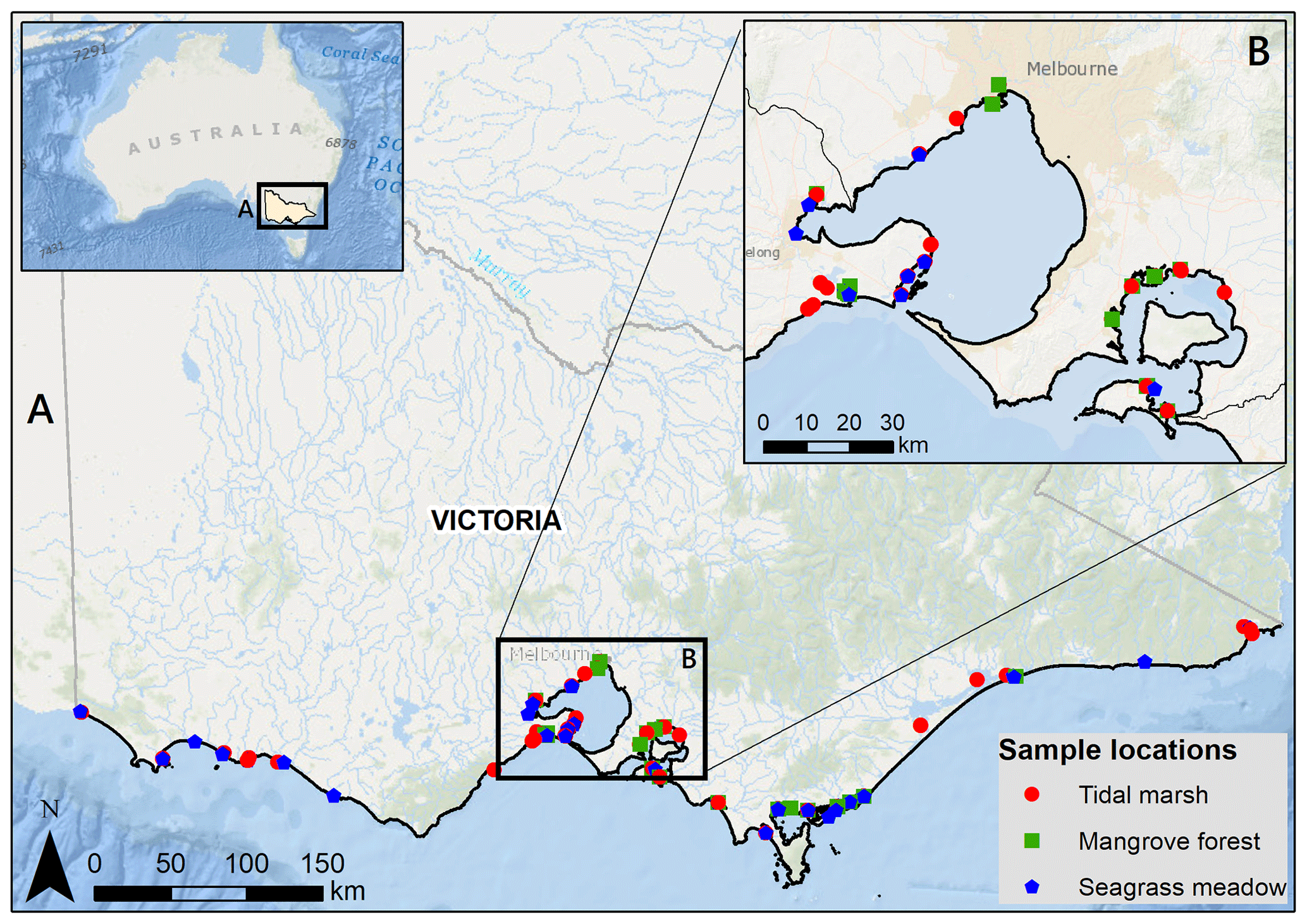
Figure 1Sample locations for 30 cm deep sediment blue C stock measurements across Victoria, Australia (a), focusing in on Port Phillip and Western Port bays (b). Service layer credits: Esri, Garmin, GEBCO, NOAA NGDC, and other contributors. Adapted from Ewers Lewis et al. (2018).
Based on the protocols by Baldock et al. (2013), a combination of diffuse reflectance Fourier transform mid-infrared (MIR) spectroscopy and elemental analysis via oxidative combustion using a LECO Trumac CN analyser was used to determine organic C contents of all samples. Previous studies have demonstrated the accuracy of using MIR to estimate organic C stocks of sediments (Baldock et al., 2013; Van De Broek and Govers, 2019; Ewers Lewis et al., 2018). MIR spectra were acquired for all samples, and a subset of 200 representative samples was selected based on a principal components analysis (PCA) of the MIR results utilizing the Kennard-Stone algorithm. Gravimetric contents of organic carbon were measured directly in the laboratory for the 200-sample subset (Baldock et al., 2013). A partial least-squares regression (PSLR) was created using a Random Cross-Validation Approach (Unscrambler 10.3, CAMO Software AS, Oslo, Norway) and used to build algorithms to predict square-root-transformed total carbon, total organic carbon, total nitrogen, and inorganic carbon for the entire dataset. The PSLR model was evaluated based on parameters from the chemometric analysis of soil properties (Bellon-Maurel et al., 2010; Bellon-Maurel and McBratney, 2011), and the relationship between measured and predicted values was assessed based on slope, offset, correlation coefficient (r), R2, the root-mean-square error (RMSE), bias, and standard error (SE) of calibration (SEC) and validation (SEP; see Ewers Lewis et al., 2018 for full details). R2 for all square-root-transformed variables was ≥0.94.
Sediment C stocks were calculated based on Howard et al. (2014). Organic C density (mg C cm−3) was calculated by multiplying organic C content (mg C g−1) by DBD (g cm−3). Linear splines were applied to each core to estimate C density for each 2 cm increment within the 30 cm core, then C densities for each interval (measured and extrapolated) were summed and converted to Mg C ha−1 to estimate total stock down to 30 cm deep for each core location.
Though it is common in the literature to sample to 1 m deep in blue C sediments, the sampling protocol used for collecting these data (Ewers Lewis et al., 2018) was designed to maximize spatial coverage of sediment C samples rather than sample entire sediment profiles (which may extend well beyond 1 m deep). Greater spatial coverage allowed us to test the relationships between a variety of potential drivers and 30 cm deep sediment C stocks on both fine and broad scales.
2.2 Generation of predictor variables
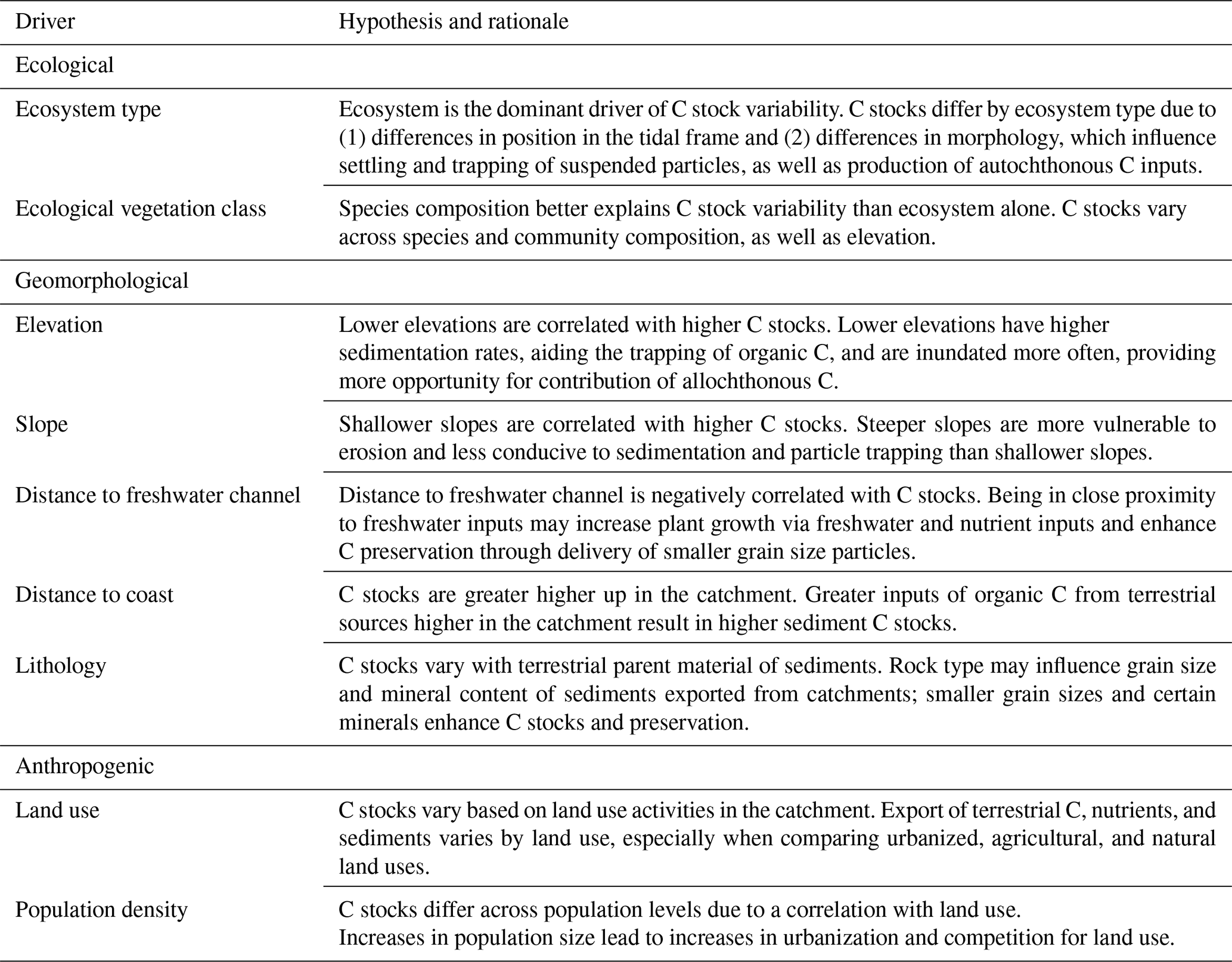
Our general approach to identifying potential drivers of 30 cm deep sediment C stock variability was to develop a predictive model based on spatially explicit environmental factors associated with our high spatial density of sediment C sampling. For clarity, we have grouped predictor variables into three categories – ecological, anthropogenic, and geomorphological – though the processes impacting C storage for each may span all three categories (Tables 1, S1 in the Supplement).
Values of predictor variables for each core were determined from spatial data either as the collective value representing activities within the catchment or based on the exact location of sample collection, depending on the variable. Geographical boundaries for catchments in Victoria were derived using high-resolution elevation data and flow accumulation models to define the spatial extents influencing fluvial and estuarine catchments (Barton et al., 2008; Fig. S1 in the Supplement). In some instances, seagrass locations sampled were beyond fluvial and estuarine catchments defined, thus we allocated characteristics of the nearest catchment region to characterize catchment influences at these locations.
Plant community was defined in two ways. First, more generally as “ecosystem” (mangrove forest, tidal marsh, or seagrass meadow) based on the plant cover where the sample was taken. Second, plant communities were further defined by either dominant species (for seagrasses, for which most were monotypic beds) or ecological vegetation class (EVC; for tidal marshes); for clarity, classification by either dominant species or EVC will be referred to as EVC from here on out. EVC was determined for each sampling location based on percentage cover of 1 m2 quadrat photos taken during sample collection. Tidal marsh EVCs sampled included coastal tussock saltmarsh, wet saltmarsh herbland, and wet saltmarsh shrubland, as described by Boon et al. (2011). Only one mangrove species is present in Victoria (the grey mangrove, Avicennia marina); therefore, further classification of this ecosystem was not used. Seagrass species sampled included Lepilaena marina, Posidonia australis, Ruppia megacarpa, Zostera muelleri, and Zostera nigricaulis.
Topographical variables for each sample location included elevation and slope. Elevation data were obtained from the Victorian Coastal Digital Elevation Model 2017 from the Cooperative Research Centre for Spatial Information. Elevation data at 2.5 m spatial resolution were used where available. Where not available (for 2.8 % of cores), 10 m spatial resolution elevation data were used to fill in the gaps. Slope was calculated from these data using the “Slope” tool in ArcMap (v. 10.2.2 for desktop). The elevation data are a composite product that integrated terrestrial and bathymetric lidar as well as multi-beam sonar data. The vertical accuracies of the data varied with sensor setup for acquisition: ±10 cm at 1 sigma (68 % conf. level) in bare ground for topographic lidar data (for the majority of our dataset), ±50 cm for bathymetric lidar, and ±<10 cm for multi-beam sonar data. Examples of spatial data used to develop models can be seen in Fig. 2. Geomorphological setting was represented for each sample location using two proxies: distance to coast and distance to freshwater channel. For each, continuous Euclidean distance rasters at 10 m resolution were created for the feature of interest using the “Euclidean Distance” tool in ArcMap. Coastline and freshwater channel data came from the State of Victoria, Department of Environment, Land, Water and Planning 2018 (Victorian Coastline 2008 and Vicmap Hydro shapefiles, respectively). The “Extract Values to Points” tool in ArcMap was used to extract raster values to each sample location.
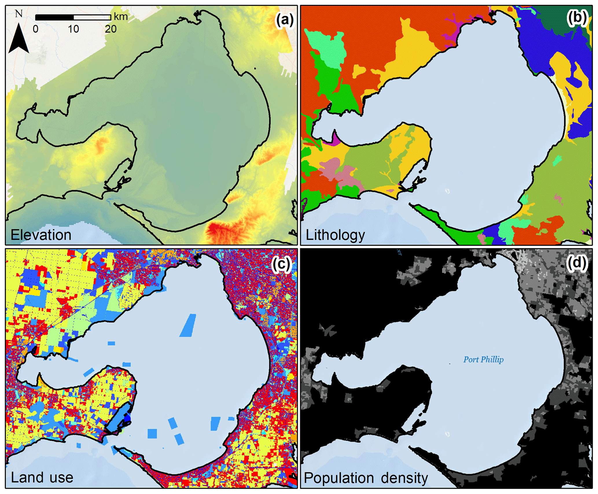
Figure 2Variability of select potential C stock drivers in Port Phillip Bay, Victoria, Australia. Raw spatial data layers were processed to define covariate values at each sample location or for the catchment of the sample location. Pictured layers include (a) elevation raster at 10 m resolution, (b) lithology polygons, (c) land use polygons, and (d) population density polygons.
Primary lithology (rock type, i.e. potential sediment parent material) was defined as the rock type covering the greatest proportion of the catchment area intersecting with sample locations. To calculate area of each lithology, the “Tabulate Area” tool was used in ArcMap based on the catchment region polygons. From the total area of each lithology in each catchment, the one with the greatest proportion was identified and input into a new field from which a new primary lithology raster was created. The Extract Values to Points tool in ArcMap was used to extract primary lithology raster values to each sample location. In total, 21 lithologies were identified in the dataset, 17 of which were identified as primary lithologies of the coastal catchments (Table S2).
Variables to assess the influence of anthropogenic processes on 30 cm deep sediment blue C stocks included three relating to land use and one relating to human population. Primary land use for the catchment was first defined as the primary land use (based on land use in individual polygons) covering the greatest proportion of the catchment area. Land use spatial data were obtained from the Victorian Land Use Information System (2014/2015) from the Victoria State Government, Department of Economic Development, Jobs, Transport and Resources. In total, nine general primary land use categories were identified in the dataset, all of which were identified as primary land uses of the coastal catchments (Table S3). The nine land use categories were pooled into three simplified categories: urbanized, agricultural, and natural. Then the areas of each within the catchment were summed and divided by total catchment area to provide the proportion of each catchment associated with those categories.
Human population densities were calculated for each catchment based on 2011 Australian census data, which were the most recent data available (Table S1). Population density was calculated for each district by dividing the population of the district by the area; this was then converted to a raster (100 m2 resolution) to calculate the mean population density for the area of each catchment.
Complete details of data availability for inputs and outputs of our models can be found in Table S10.
2.3 Model generation, selection, averaging, and validation
To identify drivers of 30 cm deep sediment C stock variability and create the best predictive model of sediment C stocks to 30 cm deep, we utilized a multi-step process based on an information theoretic approach and multi-model inference (Fig. 3). Traditional approaches have relied on identification of the “best” data-based model; however, information-theoretic approaches allow for more reliable predictions through utilization of multiple models, especially in cases where lower-ranked models may be essentially as good as the best ranked model (Burnham and Anderson, 2002; Symonds and Moussalli, 2011). Further, information theoretic model selection has been demonstrated to provide significant advantages for explaining phenomena with more complex drivers (Richards et al., 2011). Here, we first looked broadly at our variables of interest by narrowing down to the best models containing all possible variables (“global” models, as explained below) using AICC (Akaike information criteria, corrected for small sample size) to explain the variability observed in the training dataset (70 % of total C stock data; Symonds and Moussalli, 2011). From there, we identified which variables within the best global models best explained the observed variability in C stock data in order to remove unnecessary variables from the model equation (through the process of “dredging” and selecting the best subset, explained in detail below). The validity of removing unnecessary variables from the model is supported by the concept of parsimony, which suggests that models more complicated than the best model provide little benefit and should be eliminated (Burnham and Anderson, 2002; Richards, 2008). The best subset of models generated from the global models (“dredge products”) were selected based on delta AICC<2, which are viewed as essentially interchangeable with the best model (Symonds and Moussalli, 2011). Each subset of best models was used to generate an averaged model, which was tested by generating predictions of C stocks for a reserved (30 %) subset of the dataset. The best-performing model was used to generate a predictive map of C stocks to 30 cm deep for mapped blue C ecosystems in Victoria. R code for this project can be found in the Harvard Dataverse (Ewers Lewis and Young, 2020).
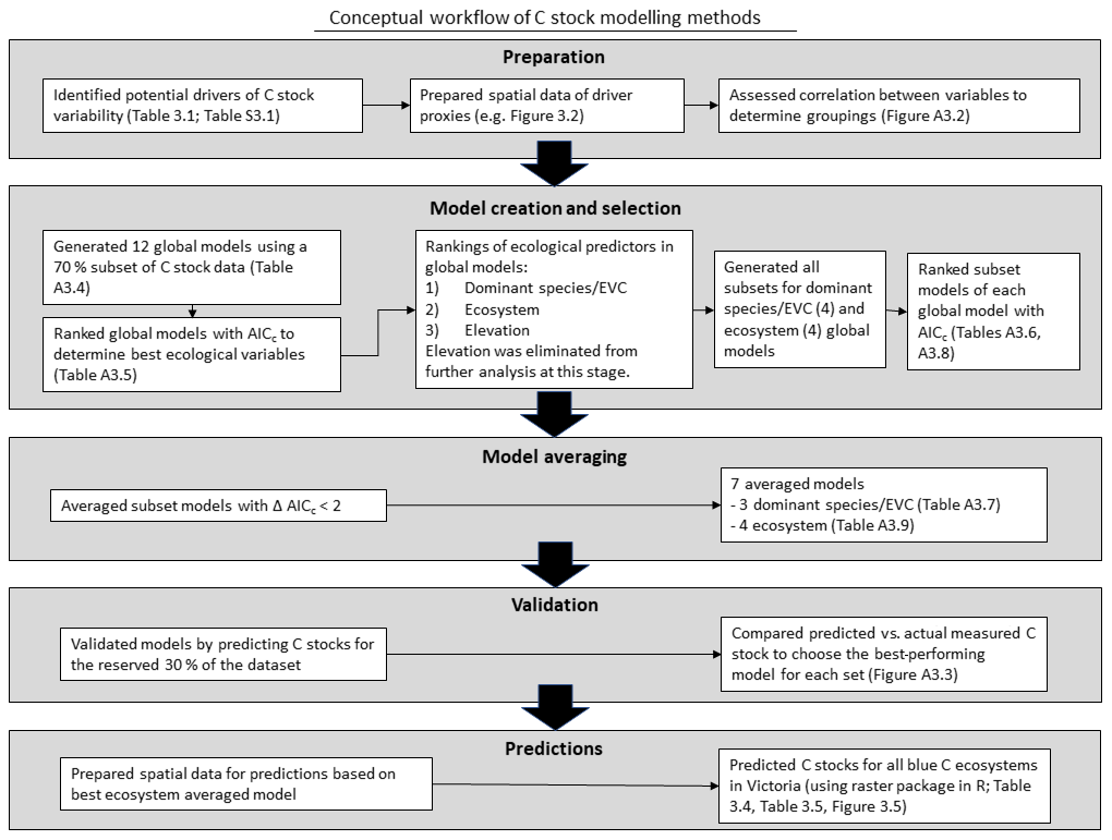
Figure 3Conceptual workflow of sediment C stock modelling methods: preparation, model creation and selection, model averaging, validation, and predictions.
To begin this process, potential ecological, geomorphological, and anthropogenic drivers were identified from the literature, and relevant proxies were extracted from available spatial data using ArcMap (Tables 1; S1). Predictor variable values derived from spatial data (along with our response variable values of C stocks) were compiled into a master data table in ArcMap. Sample rows were randomly assigned as either “training” data to build the model (70 % of the data) or “evaluating” data with which to validate the model (the remaining 30 % of the data). The training dataset was imported into R (R Core Team, 2018) for further analysis.
Table 1Hypothesized drivers of 30 cm deep sediment blue C stock variability. Drivers were grouped into three categories: (1) ecological (ecosystem type and dominant species or EVC), (2) geomorphological (elevation, slope, distance to freshwater channel, distance to coast, and lithology), and (3) anthropogenic (land use and population). A more detailed explanation of driver rationale, along with literature and spatial data references, can be found in Table S1.
Covariates were tested for correlation before composing the global models. From our 11 covariates of interest, covariate pairs were considered correlated and not used together in modelling based on a threshold value of correlation. The exception to this was covariate pairs that had a correlation value <0.4 but were still considered correlated by definition and therefore were not used together in modelling (e.g. proportion of the catchment area urbanized and proportion agricultural, Fig. S2). This resulted in four variables that did not correlate with other covariates and could be used together in all models (slope, distance to coast, distance to freshwater, and primary lithology – hereafter referred to as “geomorphological covariates”), along with correlating covariates that fell into one of two groupings: (1) ecosystem, EVC, and elevation were correlated (hereafter referred to as “ecological covariates”, and (2) mean population density, proportion urbanized land use, proportion agricultural land use, and proportion natural land use were correlated (hereafter referred to as “anthropogenic covariates”).
As a first step, we aimed to identify which models that included all (non-correlated) variables were best for explaining the variability in C stock data. Global models (i.e. containing all possible variables) were created and ranked to identify the most important drivers of C stock variability. General linear mixed-effects models (GLMMs) were generated (family = gamma, as our data were right-skewed; lme4 package v. 1.1–17; Bates et al., 2015) using all geomorphological covariates, along with one covariate each from the ecological and anthropogenic variable groups, resulting in 12 global models containing 6 covariates each (Table S4). Continuous covariates were scaled in R. Site (i.e. a single sampling area that contained from one ecosystem up to all three ecosystems) was used as a random effect in all models to account for spatial autocorrelation observed at ∼78 km.
The 12 global models were ranked using AICC (AICcmodavg package v. 2.1–1; Mazerolle, 2017; Table S5). The four best global models were chosen for further analysis based on delta AIC compared to >30 for all other models. Because the top four global models all used EVC as the ecological variable, this process was repeated for the next four best models – those that included ecosystem as the ecological predictor – to create averaged models that could be tested and used for predictions when more specific, spatially explicit plant community data (i.e. EVC) were not available.
The eight global models were “dredged” (MuMIn package v. 1.42.1; Barton, 2018) to assess the relative importance of covariates included in each model. In this context, dredging refers to the generation of a set of models that includes all possible combinations of fixed effects from the global model, containing from six to one variables (i.e. all combinations of five variables, all combinations of four variables, and so on). The dredge products of each global model (i.e. models created from dredging) were ranked using AICC and the best models (delta AICC<2) were used to produce averaged models (named based on the global model they were generated from, e.g. global model 7 → dredged and averaged → averaged model 7). Averaged models were produced using the “model.avg” function (MuMIn package v. 1.42.1; Barton, 2018). The parameter estimates for each averaged model represent the average of that parameter's values from the models in which the variable appeared (from within the subset AICC<2).
Averaged models were validated using the 30 % evaluation dataset. Due to the limitations of using cross-validation and bootstrapping on models with random effects (Colby and Bair, 2013), a direct comparison was done between predicted and actual values of the reserved dataset. The “predict” function in R was used to generate predicted C stock values for 30 cm deep sediments using each of the eight averaged models on the reserved dataset. Each set of predicted values was compared to measured 30 cm deep sediment C stock values using a linear model to compute R2 (adjusted) values. The models with the highest R2(adj) value from each set (one for “ecosystem-based” models and one for EVC-based” models) were applied to generate C stock predictions.
To test for differences in 30 cm deep sediment C stocks among EVCs, C stocks were log transformed to meet assumptions of normality and equal variances (log(Mg C ha−1)) and a one-way analysis of variance (ANOVA) was run using EVC as the factor. A Tukey's post hoc analysis was used to distinguish groupings.
2.4 Prediction of 30 cm deep sediment blue C stocks
Spatial data relevant to the best ecosystem model were compiled for prediction of current ecosystem extent sediment C stocks to 30 cm deep and included rasters for total current ecosystem extent across Victoria (all mapped tidal marsh, mangrove, and seagrass), Euclidean distance to coast, and slope. Details and source information for all spatial data can be found in Table S1. All rasters were 10 m resolution and cut to the same extent using the “Extract by Mask” tool in ArcMap. The rasters were brought into R and processed using the raster package (Hijmans, 2017). Continuous variables were scaled to match the scaled variables of the model. Rasters were then compiled into a list, stacked, and used to generate a predictive raster map (TIF file) of 30 cm deep sediment C stocks using the predict function. The C stock prediction raster (10 m resolution) was brought into ArcMap and resampled to 5 m resolution to better align to ecosystem extents. Sediment C stock values for each ecosystem extent were extracted to separate rasters and used to generate zonal statistics tables for estimating 30 cm deep sediment C stock sums and means. Rasters used for calculating C sums were converted to proper units to match map resolution using the “Map Algebra” tool (e.g. Mg C ha−1 converted to Mg C per 25 m2 raster cell). Sediment C stocks to 30 cm deep were summed for each ecosystem by catchment region, regions of interest, and the entire state. Regions of interest were identified visually as bays or estuaries hosting a substantial fraction of the state's blue C ecosystem distribution. Mapped predictions of modelled 30 cm deep sediment C stocks for this study can be found on the Harvard Dataverse (Ewers Lewis, 2020).
3.1 Drivers of 30 cm deep sediment blue C stock variability
Ranking of the 12 global models using AICC suggested the ecological variable was the most important for determining model quality (Tables S4 and S5). The top four models all contained EVC as the ecological variable, with the following four containing ecosystem, and the remaining four containing elevation. The top four models fell within a delta AICC value of ∼5.0 and under, compared to the remaining models having delta AICC values of ∼35 or more, suggesting the top four models using EVC were much better at explaining 30 cm deep sediment C stock variability than the remaining models. Within rankings for each ecological variable, anthropogenic variables in the top eight models ranked as follows, from highest to lowest importance: proportion catchment land use that is natural, proportion urbanized land use, mean population density, and proportion agricultural land use.
Dredging the top four global models and averaging the best dredge products (delta AICC<2; Table S6) resulted in only three unique sets of model-averaged parameters (Table 2; full output can be seen in Table S7). The anthropogenic variables of mean population density and proportion agricultural land use did not appear in the best models produced from dredging global models 2 and 8, respectively. Therefore, both resulted in averaged models containing the same ecological and geomorphological variables, with no anthropogenic variable, and will hereafter be referred to as averaged model 2.
Table 2Parameter estimates for averaged models containing ecological vegetation class (EVC) as the ecological variable. Parameter estimates were calculated based on averaging the best model products (delta AICC<2) resulting from dredging the top four EVC global models (global model 11, 5, 2, and 8; descriptions of global models can be found in Table S4). Note that averaged model 2 and 8 are the same because neither of the anthropogenic covariates from the global models (mean population density and proportion of agricultural land use for global models 2 and 8, respectively) appeared in the best dredge model products. EVCs are coded by ecosystem type: bold is tidal marsh, italic is mangrove, bold and italic is seagrass. Adj SE stands for adjusted standard error, RI stands for relative importance. N/A: the parameter was not included in the averaged model.

Parameter estimates from averaged models suggests EVC was the most important predictor of 30 cm deep sediment C stocks and was the only variable for which the 95 % confidence interval of the estimates did not cross 0 (Tables 2 and S7), suggesting a true effect of the variable on observed C stock variability (an estimate that included 0 means that there is potentially no impact of the variable on C stocks). Specifically, seagrasses P. australis, R. megacarpa, Z. muelleri, and Z. nigricaulis had 30 cm deep sediment C stocks that were significantly different than those of coastal tussock saltmarsh (assigned as the intercept in the model, or baseline EVC for which to compare the effect of other EVCs on C stocks), while all other tidal marsh EVCs, mangroves, and seagrass L. marina did not. This was confirmed by the ANOVA and Tukey's pairwise comparisons; there was a significant difference in 30 cm deep sediment C stocks based on EVC , p<0.001, R2(adj) = 48.77 %); tidal marsh, mangrove, and seagrass L. marina had significantly higher C stocks than seagrasses P. australis, Z. nigricaulis, and Z. muelleri (Fig. 4).
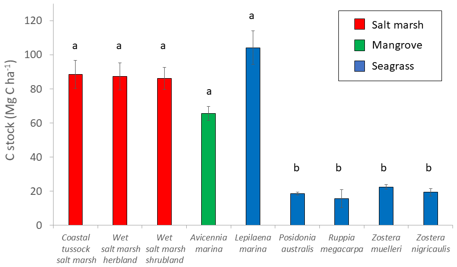
Figure 4Measured C stocks (Mg C ha−1; average ± standard error) in the top 30 cm of sediment by EVC. Bars are colour-coded by ecosystem type: red is tidal marsh, green is mangrove, and blue is seagrass. C stocks differed significantly by EVC, with higher C stocks in coastal tussock saltmarsh, wet saltmarsh herbland, wet saltmarsh shrubland, mangroves A. marina, and seagrass L. marina (group a), compared to seagrasses P. australis, Z. nigricaulis, and Z. muelleri (group b; ANOVA and Tukey pairwise comparison: ; p<0.001; R2(adj) =48.77 %). Error bars represent standard error of the mean.
Across all three EVC-averaged models, distance to coast was the next most important geomorphological predictor, ranging from 50 % to 51 % relative importance compared to EVC, followed by distance to freshwater (23 %–29 % relative importance compared to EVC), and finally slope (19 %–24 % relative importance compared to EVC). Of the two anthropogenic variables included, proportion urbanized land use was 47 % relative importance compared to EVC (averaged model 5) and proportion natural land use was 21 % relative importance compared to EVC (averaged model 11), suggesting proportion urbanized better explains variability in 30 cm deep sediment C stocks. The factor lithology did not appear in any of the best dredged models from the four global models.
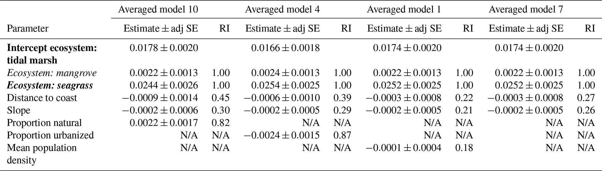
For the next four averaged models, the ecological variable, ecosystem, was again the most important covariate (relative importance = 1.00; Table 3; Tables S8 and S9). Seagrasses impacted 30 cm deep sediment C stocks differently to tidal marshes (the intercept), as evidenced by the seagrass confidence intervals not crossing zero, while mangroves were no different to tidal marshes. However, in these averaged models, anthropogenic variables had greater relative importance than geomorphological predictors, unlike the models using EVC as the ecological covariate. Proportion urbanization was still the most important anthropogenic variable, followed by proportion natural, but both had much higher relative importance (0.87 and 0.82, respectively) to the ecological variable compared to in the EVC models. Additionally, mean population density appeared in one of the averaged models, though it did not appear in any of the EVC models. Geomorphological variables, on the other hand, appeared less important in the ecosystem models than the EVC models. Relative importance of distance to coast and slope were both lower than in the previous models, and distance to freshwater channels did not appear in the top dredged models with ecosystem at all.
Table 3Parameter estimates for averaged models containing ecosystem as the ecological variable. Parameter estimates were calculated based on averaging the best model products (delta AICC<2) resulting from dredging the four global models that used ecosystem as the ecological variable (global models 10, 4, 1, and 7; descriptions of global models can be found in Table S4), combined with geomorphological and anthropogenic variables as specified. Ecosystems are coded by ecosystem type: bold is tidal marsh, italic is mangrove, bold and italic is seagrass. Adj SE stands for adjusted standard error, RI stands for relative importance. N/A: the parameter was not included in the averaged model.
3.2 Model validation
Comparison of 30 cm deep sediment C stock predictions from averaged models to actual C stock values in the 30 % evaluation dataset show that our models accounted for ∼44 %–49 % of the observed variability in 30 cm deep sediment C stock values (Fig. S3). The best three averaged models, using EVC as the ecological predictor (averaged models 11, 5, and 2), had very similar R2(adj) values (ranging 0.4829–0.4881), with the best model (averaged model 2) being the one that did not include any anthropogenic variables. The same was true when comparing models using ecosystem as the ecological variable (averaged models 10, 4, 1, and 7); the best R2(adj) was for the model with no anthropogenic variable (averaged model 7; 0.4618 compared to 0.4514, 0.4465, and 0.4566; Fig. S3).
3.3 Modelled 30 cm deep sediment blue C stocks
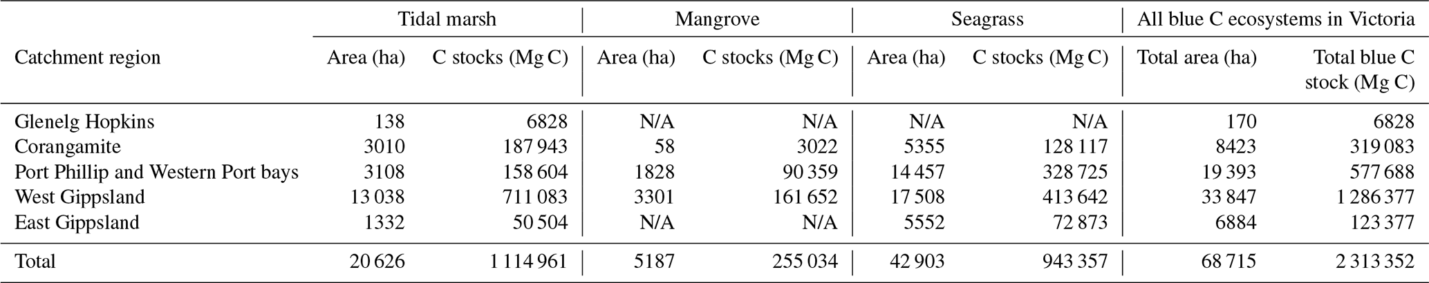
We estimated a total of over 2.31 million Mg C stored in the top 30 cm of sediments in the ∼68 700 ha of blue C ecosystems across Victoria (Table 4; Fig. 5). This estimate is based on predictions from our best averaged model that utilized ecosystem type as the ecological variable (averaged model 7), which explained 46.18 % of observed variability in C stock data and had an RMSE of 39.29. Tidal marshes stored 48.2 %, mangroves stored 11.0 %, and seagrasses stored 40.8 % of total predicted 30 cm deep sediment C stocks. Mean predicted sediment C stocks (±SD) to 30 cm deep for each ecosystem type were 57.96 (±2.90) Mg C ha−1 for tidal marsh, 50.64 (±1.35) Mg C ha−1 for mangroves, and 23.48 (±0.57) Mg C ha−1 for seagrass based on predicted C stock values in all raster cells of each ecosystem's mapped areal extent in Victoria. These 30 cm deep sediment C stock values ranged from 23.33 to 291.18, 23.34 to 77.81, and 23.33 to 73.42 Mg C ha−1 for tidal marsh, mangroves, and seagrass, respectively.
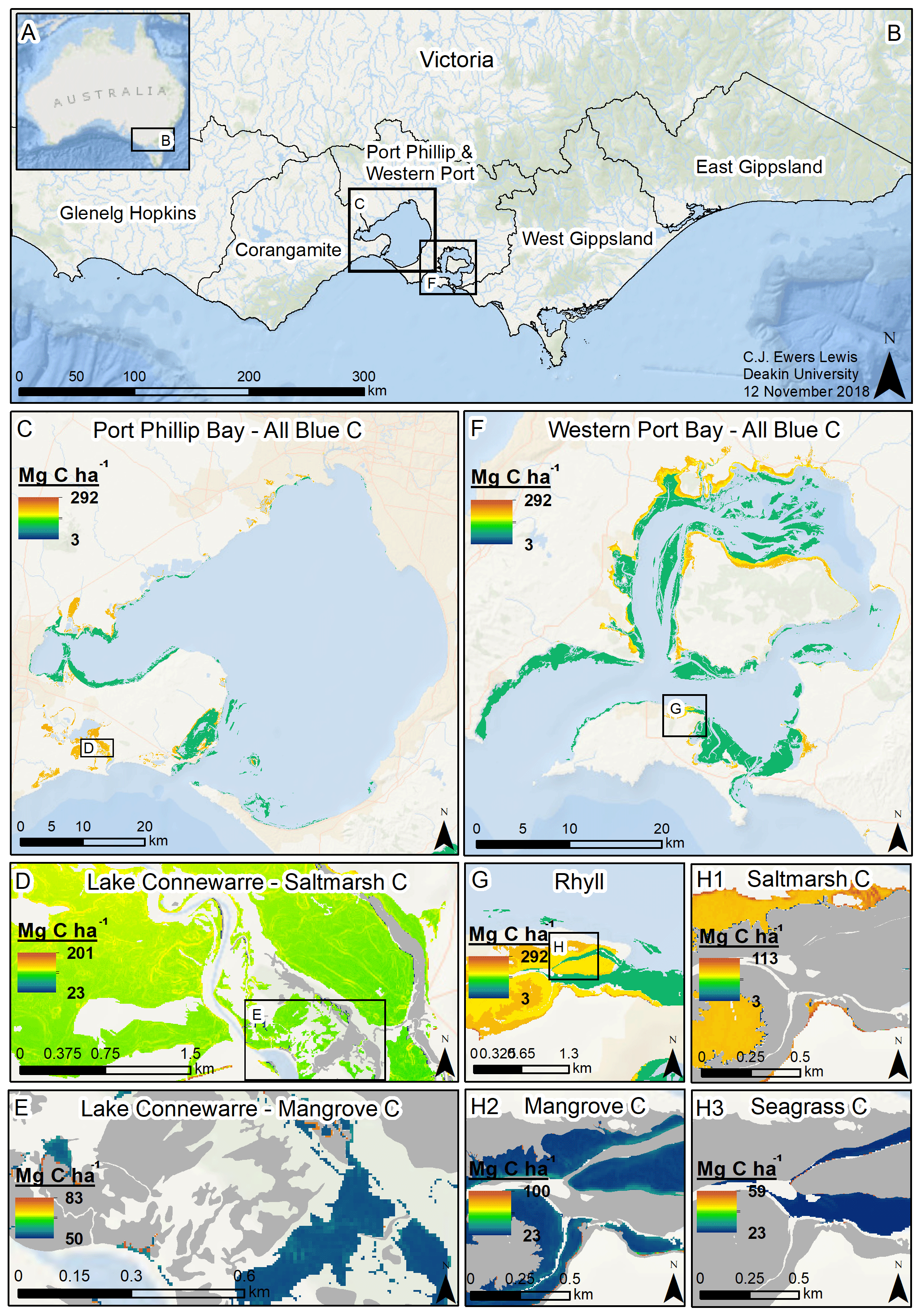
Figure 5Modelled 30 cm deep sediment blue C stocks for Victoria, Australia. Location of Victoria in Australia (a); coastal catchment regions of Victoria (b); modelled C stocks for all blue C ecosystems in Port Phillip Bay (c); modelled saltmarsh C stocks in Lake Connewarre (d); modelled mangrove C stocks in subsection of Lake Connewarre (e); modelled C stocks for all blue C ecosystems in Western Port Bay (f); modelled C stocks for all blue C ecosystems in Rhyll (Phillip Island) (g); and modelled saltmarsh C stocks (h1), mangrove C stocks (h2), and seagrass C stocks (h3) in a subsection of Rhyll. Base map service layer credits: Esri, Garmin, GEBCO, NOAA NGDC, and other contributors.
Table 4Blue C ecosystem area (ha) and modelled 30 cm deep sediment C stocks (Mg C) by catchment region and total across the state (Victoria, Australia). N/A signifies that no ecosystem extent is reflected in recent mapping in these catchment regions; therefore, C stock measurements could not be scaled up or modelled by ecosystem area.
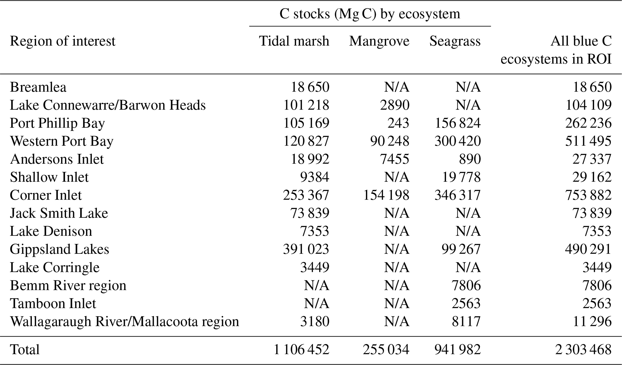
A total of 14 areas of the coast were identified as regions of interest (ROIs) and contained over 99.5 % of Victoria's total 30 cm deep sediment blue C stocks (Table 5) in 95.6 % of the state's blue C ecosystem area (∼65 700 ha). Of these regions, four of them contained over 87.6 % of total estimated 30 cm deep sediment C stocks in 86.5 % (∼59 410 ha) of the state's blue C ecosystem area. Listed from highest to lowest C stocks, they were as follows: Corner Inlet, Western Port Bay, Gippsland Lakes, and Port Phillip Bay.
Table 5Modelled 30 cm deep sediment blue C stocks (Mg C) by region of interest (ROI; listed from west to east). N/A: ecosystem does not occur in ROI.
4.1 Drivers of 30 cm deep sediment blue C stock variability
Our best model explained 48.8 % of the observed variability in 30 cm deep sediment C stocks, with the ecological variable, i.e. plant community, being the greatest predictor of C stock variability in all of the models. Plant community is related to C stocks both directly and indirectly through correlation with other variables driving C stock variability. Plant morphology may directly influence 30 cm deep sediment C stocks through the magnitude of plant biomass contributed to autochthonous C stocks and through an interaction with hydrodynamics. For example, higher C stock values in larger seagrass species, such as P. australis, are thought to be linked to both higher inputs of autochthonous C (larger rhizomes with more refractory C) and better particle trapping via a deeper canopy, which reduces water velocities and resuspension (Lavery et al., 2013). Under similar hydroperiods, saltmarsh grasses have been shown to have better sediment trapping abilities compared to mangrove trees (Chen et al., 2018), further suggesting plant traits (e.g. productivity and morphology) are an important driver of C stocks, rather than indirect impacts of inundation regimes alone.
Plant community is correlated with a number of other variables that may influence C storage, such as inundation regimes. Within and among similar ecosystems, elevation is a proxy for inundation regimes and can drive differences in C stocks. For example, in southeastern Australia, tidal marshes in the upper intertidal zone had lower C accumulation rates than mangroves, with the cause hypothesized to be that the tidal inundation was shallower, less frequent, and for shorter durations, limiting the amount of allochthonous C accumulation (Saintilan et al., 2013). This appeared to be a more important driver in C accumulation variability than the difference in biomass production between the two ecosystems (Saintilan et al., 2013), highlighting the importance of elevation in determining C stocks. In our study, elevation was correlated to ecosystem and EVC, thus the differing effects of elevation compared to vegetation community could not be teased apart without violating assumptions of non-collinearity in our models. However, the higher ranking of global models with EVC or ecosystem above those with elevation in our study suggests that the plant community itself is a better predictor of 30 cm deep sediment C stocks than simply position in the tidal frame.
Our global models specifying dominant species (for seagrass meadows) or EVC (for tidal marshes) ranked higher in our model selection than those that only specified the ecosystem (i.e. tidal marsh, mangrove, or seagrass). This ranking was supported by our model validation, in which our averaged model that best explained 30 cm deep sediment C stock variability included EVC and accounted for 48.8 % of the variability observed (Fig. S3). Still, the best averaged model containing ecosystem as the ecological predictor performed nearly as well and explained 46.2 % of the variability. These results suggest that even when specific data on species composition are not available, 30 cm deep sediment C stocks can be estimated with a similar degree of confidence based on ecosystem type, which is often a much more readily available form of data and therefore favourable for calculating sediment C stocks in data-deficient areas.
Geomorphological variables were more important than most anthropogenic variables in our models (Tables 2 and 3). Though lithology was not part of our averaged models, it is possible that its exclusion was due mostly to scale (catchment) and that it may be important when accounted for on a more local scale. Distance to coast, distance to freshwater channels, and slope all appeared in the averaged models using EVC, with distance to coast being most important. However, in models using ecosystem, distance to freshwater channels was no longer important enough to appear in the averaged models, and the anthropogenic variables, proportion urbanized and proportion natural, were more important than any of the geomorphological variables. Model validation revealed that the best predictions for either set of models (those using EVC and those using ecosystem as the ecological variable) came from the model that did not include any anthropogenic variables.
Although our models suggest anthropogenic variables have little impact on 30 cm deep sediment C stocks, it is more likely that anthropogenic variables are impacting processes we could not measure. For example, excess nutrients resulting from certain land uses may stress plants to the point of affecting survival and therefore sediment stability (Macreadie et al., 2017b). Without measuring changes to ecosystem distribution or sediment thickness (i.e. erosion), we could not pick up on these sediment C losses. Similarly, though enhanced sedimentation rates may increase C burial in catchments with certain land uses (e.g. high population density or high area of agriculture; Yang et al., 2003), this addition to C stocks would be reflected in sequestration rate, which we did not measure in this study.
Proxies for the drivers of sediment C stock variability can be quantified and described for modelling in numerous ways. Though we maximized our ability to choose variables representing meaningful relationships with 30 cm deep sediment C stocks by alternating the forms of the anthropogenic variables tested in our models (i.e. proportion urban vs. proportion agriculture vs. proportion natural vs. mean population density), it may be beneficial to incorporate more direct measures of anthropogenic impacts in C stock modelling, such as nutrients and suspended particulate organic matter coming from catchments.
We also aimed to maximize our ability to capture relationships between contemporary drivers and sediment C stocks by utilizing sediment C stock data to only 30 cm deep, a sediment horizon more directly impacted by recent environmental conditions compared to deeper stocks due to age. Based on previously estimated sediment accretion rates in blue C ecosystems in the study region (averaging 2.51 to 2.66 mm yr−1 in tidal marshes, Ewers Lewis et al., 2019; Rogers et al., 2006a; and 7.14 mm yr−1 in mangroves, Rogers et al., 2006a), the top 30 cm of sediment represents roughly ∼113–120 years of accretion in Victorian tidal marshes and ∼42 years of accretion in Victorian mangroves. These timescales suggest sediments depths utilized in this study are more appropriate for assessing the impacts of modern environmental conditions on sediment C stocks compared to metre-deep stocks, which can be thousands of years old (e.g. Ewers Lewis et al., 2019). Using 30 cm deep sediment C stocks also allows us to be more confident that the vegetation present now has been there during the time of sediment accretion, unlike deeper sediments that are thousands of years old and for which it is difficult to determine what vegetation, if any, was present at the time of accretion.
The variability in 30 cm deep sediment C stocks that could not be explained by our modelling may also be related to the inherent challenges surrounding spatial and temporal matching of driver proxies and sediment C stock measurements; the relationship between 30 cm deep sediment C stocks and contemporary environmental settings can be represented more accurately for some variables over others.
Ecosystem type was a relatively powerful predictor of 30 cm deep sediment C stock variability in our study and this is likely due, in part, to the direct relationship between vegetation and surface sediments. In most vegetated ecosystems, the majority of underground plant biomass and microbial activity exists within the top 20 cm of soils (Trumbore, 2009). For saltmarsh, it has been demonstrated that the top 30 cm of sediment are directly impacted by current vegetation (Owers et al., 2016). Therefore, using 30 cm deep sediment C stock measurements allowed us to target the portion of the sediment profile most likely to be influenced by current vegetation.
The portion of recently accreted sediments influenced by contemporary anthropogenic drivers is harder to identify than that influenced by ecosystem vegetation. Based on estimated accretion rates for this region from the literature (Ewers Lewis et al., 2019; Rogers et al., 2006b), 30 cm deep sediments would have taken an average of ∼80 years to accumulate in Victoria (∼117 years in tidal marsh and ∼42 years in mangroves). Though sedimentation rates vary over time, they are relatively steady in comparison to changes in anthropogenic drivers, such as land use change, which can happen abruptly. This means that modern-day maps of land use, though useful for looking at the general impact of human activities on ecosystem processes, may be more useful for relating to variability in sediment C stocks when the data are assessed at finer temporal resolutions. For example, comparing land use area data across various time periods with C densities in aged bands of sediment could help capture the pulse effects of sudden land use changes in narrower sediment horizons representative of the same time periods. In this study, the effects of land-use change may have been too diluted within the 30 cm horizons to relate to impacts on sediment C stock.
Spatially, anthropogenic variables are also difficult to assign to particular ecosystem locations or depths. Many blue C ecosystems in Victoria are located in coastal embayments and receive inputs from multiple catchments, making the influence of specific areas of land-use or population changes difficult to track to specific ecosystem locations. Modern-day factors influencing vegetation can also have impacts on C stocks deeper than the sediments we measured. The effects of underground biomass on sediment C stocks can extend beyond the top 30 cm, and in fact new C inputs and active C cycling by microbial communities can occur as deep as underground roots extend (Trumbore, 2009). These new C additions (and fluxes) at depth fall outside the general pattern of sediment C decay down-core in vegetated ecosystems (Trumbore, 2009), which has previously allowed for linear or logarithmic regressions to be used to extrapolate 1 m deep C contents from shallow (e.g. 30–50 cm deep) sediment C data (Macreadie et al., 2017a; Serrano et al., 2019). The activity of underground biomass and microbes at depth, when considered over space and time, may account for large C fluxes. The influence of anthropogenic activities, such as land use changes, on these processes via impacts to vegetation may largely go unnoticed based on current methods (Trumbore, 2009), both in this study and in blue C stock assessments on larger scales. We suggest further research to understand the dynamics of active C cycling at sediment depths traditionally considered stable.
Another limitation to C stock modelling is knowledge of environmental features that may be important in influencing C storage but are generally not monitored. For example, the maturity of a blue C ecosystem can affect C storage and composition (Kelleway et al., 2015). Within a single saltmarsh species, the maturity of the system is a major factor determining the role of the marsh as a C sink. Mature systems of Spartina maritime have higher C retention – via higher below ground production, slower decomposition rate, and higher C content in sediments – than younger S. maritime marsh systems (Sousa et al., 2010b). Mature marshes have also been observed to have greater contributions of allochthonous C storage over time, while younger marshes predominantly have autochthonous organic matter signatures (Chen et al., 2016; Tu et al., 2015). Long-term mapping of blue C ecosystems could be beneficial for tracking maturity of vegetation for C stock modelling as well as reducing the error in C stock measurements associated with changes to blue C ecosystem area.
Finally, we suggest future studies examine the relationship between the drivers we have described and individual blue C ecosystem types in order to further refine sediment blue C stock modelling. With a large dataset from a single ecosystem, relationships may be identified that were overshadowed in this study by the inclusion of all three ecosystems. For example, because elevation correlated with our two ecological variables, it was not included in our best models. However, within a single ecosystem, elevation may be an important driver of sediment C stock variability due to its relationship with inundation regimes (Chen et al., 2016; Chmura et al., 2003; Chmura and Hung, 2004).
4.2 Modelled 30 cm deep sediment blue C stocks
Our estimate of 2.31 million Mg C stored in the top 30 cm of sediment in all blue C ecosystems in Victoria was about 20 % lower than that of Ewers Lewis et al. (2018), who estimated 2.91 million Mg C based on the same C stock data but calculated total stocks based on average C stock values and ecosystem extent in each of the five coastal catchments. These results suggest that modelling 30 cm deep sediment C stocks based on environmental drivers may reduce the chances of overestimating sediment C stocks by better accounting for fine-scale variability. Our modelled 30 cm deep sediment C stock estimates support our earlier findings that tidal marshes store more C than any other blue C ecosystem in Victoria. Our estimates are now refined in that modelled stocks suggest tidal marshes store closer to 48 % (rather than 53 %) and seagrasses store closer to 41 % (rather than 36 %) of total 30 cm deep sediment blue C stocks (Ewers Lewis et al., 2018). Our original estimate of mangrove contribution to total blue C was supported by our modelling: by either method, we estimated mangroves to store 11 % of Victoria's 30 cm deep sediment blue C stocks.
It is important to emphasize here that total sediment depths in blue C ecosystems can vary greatly, and are commonly deeper than 30 cm. Blue C ecosystems can have sediments up to several metres deep (e.g. Lavery et al., 2013; Scott and Greenberg, 1983), suggesting the estimates of C stocks measured here are conservative. In spite of these limitations, 30 cm deep sediment C stock estimates give us valuable knowledge about the sediment C pool most vulnerable to disturbance and how it may be impacted by environmental drivers.
In examining C stocks within ROIs, i.e. areas of the coast containing substantial distributions of blue C ecosystems, we found that just four of the 14 ROIs housed nearly 88 % of 30 cm deep sediment blue C stocks in the state, a direct reflection of the large proportion of blue C ecosystem area in these regions (nearly 87 % of the state's total blue C area). This trend appears to be driven by the presence of extensive seagrass sediment C stocks (Table 5) in these four regions, accompanied by extensive tidal marsh sediment C stocks. This result has important implications for management of coastal blue C. In cases where resources are limited, identification of areas housing major blue C sinks, in conjunction with evaluation of other ecosystem services, can help provide insight to guide conservation strategies. For example, strategies to conserve tidal marshes in the four major ROIs could serve the additional purpose of helping to preserve the adjacent seagrass meadows via facilitation; tidal marshes serve as filters of excess nutrients coming down from the catchment (Nelson and Zavaleta, 2012) that may otherwise cause a loss of seagrass beds due to light reduction resulting from the growth of algal epiphytes, macroalgae, and phytoplankton (Burkholder et al., 2007). Further, our mapping of within-ecosystem-patch variability in 30 cm deep sediment C stocks is an important output for facilitating management actions on an applicable level, allowing prioritization of particular parts of an ecosystem patch for conservation when necessary.
In this study, we had the unique opportunity to assess a large regional dataset of 30 cm deep sediment blue C stocks to explore the influence of ecological, geomorphological, and anthropogenic variables in driving sediment blue C stock variability. Because of the high spatial resolution of sampling within similar latitudes we were able to focus on variables driving differences in 30 cm deep sediment C stocks within catchments. We found that plant community was most important for determining 30 cm deep sediment C stocks and that combining this variable with geomorphological variables relating to position in the catchment allowed us to model stocks at a fine spatial resolution. Identification and mapping of these dense 30 cm deep sediment blue C sinks in Victoria, in conjunction with evaluation of other ecosystem services, will be useful for conservation management regionally, e.g. through the identification of hotspots for protection and key locations for restoration efforts. We recommend these methods be tested in other areas of the globe to determine whether they may be applicable for identifying relationships between potential environmental drivers and sediment blue C stocks and creating predictive sediment C stock models and maps for blue C ecosystems at scales relevant to resource management applications in other regions.
The data associated with this study are accessible through the Harvard Dataverse: (1) sediment carbon stock data (Ewers Lewis et al., 2020, https://doi.org/10.7910/DVN/6PFBO0), (2) R code (Ewers Lewis and Young, 2020 https://doi.org/10.7910/DVN/0WKEHJ), and (3) blue carbon stock predictions map of Victoria, Australia (Ewers Lewis, 2020, https://doi.org/10.7910/DVN/UDOAUT).
The supplement related to this article is available online at: https://doi.org/10.5194/bg-17-2041-2020-supplement.
CJEL, DI, MAY, and PIM conceived the study. CJEL, JAB, BH, JS, PEC, and PIM produced the input carbon data for the model. CJEL and MAY wrote the code. CJEL analysed the data, performed the calculations, and produced the GIS data and maps. CJEL prepared the paper with contributions from all authors.
The authors declare that they have no conflict of interest.
We thank Parks Victoria and the Victorian Coastal Catchment Management Authorities (CMAs) for their support and funding: Marty Gent and Glenelg Hopkins CMA, Chris Pitfield and Corangamite CMA, Emmaline Froggatt and Port Phillip Western Port CMA, Belinda Brennan and West Gippsland CMA, and Rex Candy and East Gippsland CMA. Carolyn J. Ewers Lewis also thanks the University of Technology Sydney for scholarship support.
This research has been supported by Parks Victoria; the Victorian Coastal Management Authorities of Glenelg Hopkins, Corangamite, Port Phillip and Western Port, West Gippsland, and East Gippsland; and the Australian Research Council (DECRA Fellowship no. DE130101084 and Linkage Project no. LP160100242).
This paper was edited by Steven Bouillon and reviewed by two anonymous referees.
Armitage, A. R. and Fourqurean, J. W.: Carbon storage in seagrass soils: long-term nutrient history exceeds the effects of near-term nutrient enrichment, Biogeosciences, 13, 313–321, https://doi.org/10.5194/bg-13-313-2016, 2016.
Atwood, T. B., Connolly, R. M., Almahasheer, H., Carnell, P. E., Duarte, C. M., Ewers Lewis, C. J., Irigoien, X., Kelleway, J. J., Lavery, P. S., Macreadie, P. I., Serrano, O., Sanders, C. J., Santos, I., Steven, A. D. L., and Lovelock, C. E.: Global patterns in mangrove soil carbon stocks and losses, Nat. Clim. Change, 7, 523–528, https://doi.org/10.1038/NCLIMATE3326, 2017.
Baldock, J. A., Hawke, B., Sanderman, J., and MacDonald, L. M.: Predicting contents of carbon and its component fractions in Australian soils from diffuse reflectance mid-infrared spectra, Soil Res., 51, 577–595, https://doi.org/10.1071/SR13077, 2013.
Barton, J., Pope, A., Quinn, G., and Sherwood, J.: Identifying threats to the ecological condition of Victorian estuaries, Department of Sustainability and Environment Technical Report, Warrnambool, Victoria, 1–54, 2008.
Barton, K.: MuMIn: Multi-Model Inference, available at: https://cran.r-project.org/package=MuMIn, last access: 12 January 2018.
Bates, D., Mächler, M., Bolker, B., and Walker, S.: Fitting Linear Mixed-Effects Models using lme4, J. Stat. Softw., 67, 1–48, https://doi.org/10.18637/jss.v067.i01, 2015.
Bellon-Maurel, V. and McBratney, A.: Near-infrared (NIR) and mid-infrared (MIR) spectroscopic techniques for assessing the amount of carbon stock in soils – Critical review and research perspectives, Soil Biol. Biochem., 43, 1398–1410, https://doi.org/10.1016/j.soilbio.2011.02.019, 2011.
Bellon-Maurel, V., Fernandez, E., Palagos, B., Roger, J., and McBratney, A.: Prediction of soil attributes by NIR/MIR spectroscopy. Coming back to statistics fundamentals to improving prediction accuracy, Trends Anal. Chem., 29, 1073–1081, 2010.
Boon, P. I., Allen, T., Brook, J., Carr, G., Frood, D., Harty, C., Hoye, J., Mcmahon, Andrew Mathews, S., Rosengren, N., Sinclair, S., White, M., and Yugovic, J.: Mangroves and coastal saltmarsh of Victoria: distribution, condition, threats and management, Institute for Sustainability and Innovation, Victoria University, Melbourne, 2011.
Bouillon, S., Dahdouh-Guebas, F., Rao, A. V. V. S., Koedam, N., and Dehairs, F.: Sources of organic carbon in mangrove sediments: variability and possible ecological implications, Hydrobiologia, 495, 33–39, 2003.
Burkholder, J. M., Tomasko, D. A., and Touchette, B. W.: Seagrasses and eutrophication, J. Exp. Mar. Biol. Ecol., 350, 46–72, https://doi.org/10.1016/j.jembe.2007.06.024, 2007.
Burnham, K. P. and Anderson, D. R.: Model Selection and Multimodel Inference: A Practical Information-TheoreticApproach, 2nd Edn., Springer, New York, 1–22, 2002.
Chen, S., Torres, R., and Goñi, M. a.: The Role of Salt Marsh Structure in the Distribution of Surface Sedimentary Organic Matter, Estuar. Coast., 39, https://doi.org/10.1007/s12237-015-9957-z, 2016.
Chen, Y., Li, Y., Thompson, C., Wang, X., Cai, T., and Chang, Y.: Differential sediment trapping abilities of mangrove and saltmarsh vegetation in a subtropical estuary, Geomorphology, 318, 270–282, https://doi.org/10.1016/j.geomorph.2018.06.018, 2018.
Chmura, G. L. and Hung, G. A.: Controls on Salt Marsh Accretion: A Test in Salt Marshes of Eastern Canada, Estuaries, 27, 70–81, 2004.
Chmura, G. L., Anisfeld, S. C., Cahoon, D. R., and Lynch, J. C.: Global carbon sequestration in tidal, saline wetland soils, Global Biogeochem. Cy., 17, 1111, https://doi.org/10.1029/2002GB001917, 2003.
Colby, E. and Bair, E.: Cross-validation for nonlinear mixed effects models, J. Pharmacokinet. Pharmacodyn., 40, 243–252, https://doi.org/10.1007/s10928-013-9313-5, 2013.
Connor, R. F., Chmura, G. L., and Beecher, C. B.: Carbon accumulation in Bay of Fundy salt marshes: Implications for restoration of reclaimed marshes, Global Biogeochem. Cy., 15, 943–954, 2001.
Ewers Lewis, C. J.: 2020, Model Predictions Map: 30-cm Deep Sediment Blue Carbon Stocks for Victoria, Australia, https://doi.org/10.7910/DVN/UDOAUT, Harvard Dataverse, V1, 2020.
Ewers Lewis, C. J. and Young, M.: R Code for 30-cm Sediment Blue Carbon Stock Modelling, https://doi.org/10.7910/DVN/0WKEHJ, Harvard Dataverse, V1, 2020.
Ewers Lewis, C. J., Carnell, P., and Macreadie, P.: Victoria Coastal Blue Carbon Sediment Dataset, https://doi.org/10.7910/DVN/6PFBO0, Harvard Dataverse, V1, 2020.
Ewers Lewis, C. J., Carnell, P. E., Sanderman, J., Baldock, J. A., and Macreadie, P. I.: Variability and Vulnerability of Coastal “Blue Carbon” Stocks: A Case Study from Southeast Australia, Ecosystems, 21, 263–247, https://doi.org/10.1007/s10021-017-0150-z, 2018.
Ewers Lewis, C. J., Baldock, J. A., Hawke, B., Gadd, P. S., Zawadzki, A., Heijnis, H., Jacobsen, G. E., Rogers, K., and Macreadie, P. I.: Impacts of land reclamation on tidal marsh “blue carbon” stocks, Sci. Total Environ., 672, 427–437, https://doi.org/10.1016/j.scitotenv.2019.03.345, 2019.
Hijmans, R. J.: raster: Geographic Data Analysis and Modeling, available at: https://cran.r-project.org/package=raster (last access: 12 January 2018), 2017.
Howard, J., Hoyt, S., Isensee, K., Pidgeon, E., and Telszewski, M. (Eds.): Coastal Blue Carbon: Methods for assessing carbon stocks and emissions factors in mangroves, tidal salt marshes, and seagrass meadows, Conservation International, Intergovernmental Oceanographic Commission of UNESCO, International Union for Conservation of Nature, Arlington, Virginia, USA, 39–66, 2014.
Kearns, P. J., Bulseco-Mckim, A. N., Hoyt, H., Angell, J. H., and Bowen, J. L.: Nutrient Enrichment Alters Salt Marsh Fungal Communities and Promotes Putative Fungal Denitrifiers, Microb. Ecol., 77, 358–369, https://doi.org/10.1007/s00248-018-1223-z, 2018.
Kelleway, J. J., Saintilan, N., Macreadie, P. I., Skilbeck, C. G., Zawadzki, A., and Ralph, P. J.: Seventy years of continuous encroachment substantially increases “blue carbon” capacity as mangroves replace intertidal salt marshes, Glob. Change Biol., 22, 1097–1109, https://doi.org/10.1111/gcb.13158, 2015.
Kelleway, J. J., Saintilan, N., Macreadie, P. I., and Ralph, P. J.: Sedimentary Factors are Key Predictors of Carbon Storage in SE Australian Saltmarshes, Ecosystems, 19, 865–880, https://doi.org/10.1007/s10021-016-9972-3, 2016.
Kelleway, J. J., Saintilan, N., Macreadie, P. I., Baldock, J. A., and Ralph, P. J.: Sediment and carbon deposition vary among vegetation assemblages in a coastal salt marsh, Biogeosciences, 14, 3763–3779, https://doi.org/10.5194/bg-14-3763-2017, 2017.
Lavery, P. S., Mateo, M.-Á., Serrano, O., and Rozaimi, M.: Variability in the carbon storage of seagrass habitats and its implications for global estimates of blue carbon ecosystem service, PLoS One, 8, e73748, https://doi.org/10.1371/journal.pone.0073748, 2013.
Liu, S., Jiang, Z., Wu, Y., Zhang, J., Arbi, I., Ye, F., Huang, X., and Macreadie, P. I.: Effects of nutrient load on microbial activities within a seagrass-dominated ecosystem: Implications of changes in seagrass blue carbon, Mar. Pollut. Bull., 117, 214–221, https://doi.org/10.1016/j.marpolbul.2017.01.056, 2017.
Lovelock, C. E., Atwood, T., Baldock, J., Duarte, C. M., Hickey, S., Lavery, P. S., Masque, P., Macreadie, P. I., Ricart, A. M., Serrano, O., and Steven, A.: Assessing the risk of carbon dioxide emissions from blue carbon ecosystems, Front. Ecol. Environ., 15, 257–265, https://doi.org/10.1002/fee.1491, 2017.
Macreadie, P., Ollivier, Q., Kelleway, J., Serrano, O., Carnell, P., Ewers Lewis, C., Atwood, T., Sanderman, J., Baldock, J., Connolly, R., Duarte, C., Lavery, P., Steven, A., and Lovelock, C.: Carbon sequestration by Australian tidal marshes, Sci. Rep., 7, 44071, https://doi.org/10.1038/srep44071, 2017a.
Macreadie, P. I., Nielsen, D. A., Kelleway, J. J., Atwood, T. B., Seymour, J. R., Petrou, K., Connolly, R. M., Thomson, A. C., Trevathan-Tackett, S. M., and Ralph, P. J.: Can we manage coastal ecosystems to sequester more blue carbon?, Front Ecol Env., 15, 206–213, https://doi.org/10.1002/fee.1484, 2017b.
Mayer, L. M.: Relationships between mineral surfaces and organic carbon concentrations in soil and sediments, Chem. Geol., 114, 347–363, https://doi.org/10.1016/0009-2541(94)90063-9, 1994.
Mazarrasa, I., Marbà, N., Garcia-Orellana, J., Masqué, P., Arias-Ortiz, A., and Duarte, C. M.: Effect of environmental factors (wave exposure and depth) and anthropogenic pressure in the C sink capacity of Posidonia oceanica meadows, Limnol. Oceanogr., 62, 1436–1450, https://doi.org/10.1002/lno.10510, 2017.
Mazerolle, M. J.: AICcmodavg: Model selection and multimodel inference based on (Q)AIC(c), available at: https://cran.r-project.org/package=AICcmodavg (last access: 12 January 2018), 2017.
Mcleod, E., Chmura, G. L., Bouillon, S., Salm, R., Björk, M., Duarte, C. M., Lovelock, C. E., Schlesinger, W. H., and Silliman, B. R.: A blueprint for blue carbon: toward an improved understanding of the role of vegetated coastal habitats in sequestering CO2, Front. Ecol. Environ., 9, 552–560, https://doi.org/10.1890/110004, 2011.
Nellemann, C., Corcoran, E., Duarte, C. M., Valdes, L., Young, C. D., Fonseca, L., and Grimsditch, G. (Eds.): Blue carbon: the role of healthy oceans in binding carbon: a rapid response assessment. UNEP/Earthprint, 2009.
Nelson, J. L. and Zavaleta, E. S.: Salt Marsh as a Coastal Filter for the Oceans: Changes in Function with Experimental Increases in Nitrogen Loading and Sea-Level Rise, edited by J. Cebrian, PLoS One, 7, e38558, https://doi.org/10.1371/journal.pone.0038558, 2012.
Osland, M. J., Gabler, C. A., Grace, J. B., Day, R. H., McCoy, M. L., McLeod, J. L., From, A. S., Enwright, N. M., Feher, L. C., Stagg, C. L., and Hartley, S. B.: Climate and plant controls on soil organic matter in coastal wetlands, Glob. Change Biol., 24, 5361–5379, https://doi.org/10.1111/gcb.14376, 2018.
Owers, C. J., Rogers, K., and Woodroffe, C. D.: Identifying spatial variability and complexity in wetland vegetation using an object-based approach, Int. J. Remote Sens., 37, 4296–4316, https://doi.org/10.1080/01431161.2016.1211349, 2016.
Quiros, T. E. A. L., Croll, D., Tershy, B., Fortes, M. D., and Raimondi, P.: Land use is a better predictor of tropical seagrass condition than marine protection, Biol. Conserv., 209, 454–463, https://doi.org/10.1016/j.biocon.2017.03.011, 2017.
R Core Team: R: A Language and Environment for Statistical Computing, available at: https://www.r-project.org/, last access: 12 January 2018.
Ricart, A. M., York, P. H., Rasheed, M. A., Pérez, M., Romero, J., Bryant, C. V., and Macreadie, P. I.: Variability of sedimentary organic carbon in patchy seagrass landscapes, Mar. Pollut. Bull., 100, 476–482, https://doi.org/10.1016/j.marpolbul.2015.09.032, 2015.
Richards, S. A.: Dealing with overdispersed count data in applied ecology, J. Appl. Ecol., 45, 218–227, https://doi.org/10.1111/j.1365-2664.2007.01377.x, 2008.
Richards, S. A., Whittingham, M. J., and Stephens, P. A.: Model selection and model averaging in behavioural ecology: The utility of the IT-AIC framework, Behav. Ecol. Sociobiol., 65, 77–89, https://doi.org/10.1007/s00265-010-1035-8, 2011.
Rogers, K., Wilton, K. M., and Saintilan, N.: Vegetation change and surface elevation dynamics in estuarine wetlands of southeast Australia, Estuar. Coast. Shelf Sci., 66, 559–569, https://doi.org/10.1016/j.ecss.2005.11.004, 2006a.
Rogers, K., Wilton, K. M., and Saintilan, N.: Vegetation change and surface elevation dynamics in estuarine wetlands of southeast Australia, Estuar. Coast. Shelf Sci., 66, 559–569, https://doi.org/10.1016/j.ecss.2005.11.004, 2006b.
Rovai, S., Twilley, R. R., Castaamp, E., Riul, P., Cifuentes-Jara, M., Manrow-Villalobos, M., Horta, P. A., Simonassi, C., Fonseca, A. L., and Pagliosa, P. R.: Global controls on carbon storage in mangrove soils, Nat. Clim. Change, 8, 534–538, https://doi.org/10.1038/s41558-018-0162-5, 2018.
Saintilan, N., Rogers, K., Mazumder, D., and Woodroffe, C.: Allochthonous and autochthonous contributions to carbon accumulation and carbon store in southeastern Australian coastal wetlands, Estuar. Coast. Shelf Sci., 128, 84–92, https://doi.org/10.1016/j.ecss.2013.05.010, 2013.
Sanderman, J., Hengl, T., Fiske, G., Solvik, K., Adame, M. F., Benson, L., Bukoski, J. J., Carnell, P., Cifuentes-Jara, M., Donato, D., Duncan, C., Eid, E. M., Ermgassen, P., Ewers Lewis, C. J., Glass, L., Gress, S., Jardine, S. L., Jones, T., Macreadie, P., Nsombo, E. N., Rahman, M. M., Sanders, C., Spalding, M., and Landis, E.: A global map of mangrove forest soil carbon at 30 m spatial resolution, Environ. Res. Lett., 13, 055002, https://doi.org/10.1088/1748-9326/aabe1c, 2018.
Sanders, C. J., Maher, D. T., Tait, D. R., Williams, D., Holloway, C., Sippo, J. Z., and Santos, I. R.: Are global mangrove carbon stocks driven by rainfall?, J. Geophys. Res.-Biogeo., 121, 2600–2609, https://doi.org/10.1002/2016JG003510, 2016.
Scott, D. B. and Greenberg, D. A.: Relative sea-level rise and tidal development in the Fundy tidal system, Can. J. Earth Sci., 20, 1554–1564, https://doi.org/10.1139/e83-145, 1983.
Serrano, O., Lavery, P. S., Duarte, C. M., Kendrick, G. A., Calafat, A., York, P. H., Steven, A., and Macreadie, P. I.: Can mud (silt and clay) concentration be used to predict soil organic carbon content within seagrass ecosystems?, Biogeosciences, 13, 4915–4926, https://doi.org/10.5194/bg-13-4915-2016, 2016a.
Serrano, O., Lavery, P., Masque, P., Inostroza, K., Bongiovanni, J., and Duarte, C.: Seagrass sediments reveal the long-term deterioration of an estuarine ecosystem, Glob. Change Biol., 22, 1523–1531, https://doi.org/10.1111/gcb.13195, 2016b.
Serrano, O., Lovelock, C. E., B. Atwood, T., Macreadie, P. I., Canto, R., Phinn, S., Arias-Ortiz, A., Bai, L., Baldock, J., Bedulli, C., Carnell, P., Connolly, R. M., Donaldson, P., Esteban, A., Ewers Lewis, C. J., Eyre, B. D., Hayes, M. A., Horwitz, P., Hutley, L. B., Kavazos, C. R. J., Kelleway, J. J., Kendrick, G. A., Kilminster, K., Lafratta, A., Lee, S., Lavery, P. S., Maher, D. T., Marbà, N., Masque, P., Mateo, M. A., Mount, R., Ralph, P. J., Roelfsema, C., Rozaimi, M., Ruhon, R., Salinas, C., Samper-Villarreal, J., Sanderman, J., J. Sanders, C., Santos, I., Sharples, C., Steven, A. D. L., Cannard, T., Trevathan-Tackett, S. M., and Duarte, C. M.: Australian vegetated coastal ecosystems as global hotspots for climate change mitigation, Nat. Commun., 10, 4313, https://doi.org/10.1038/s41467-019-12176-8, 2019.
Siikamäki, J., Sanchirico, J. N., Jardine, S., McLaughlin, D., and Morris, D.: Blue carbon: coastal ecosystems, their carbon storage, and potential for reducing emissions, Environ. Sci. Policy Sustain. Dev., 55, 14–29, https://doi.org/10.1080/00139157.2013.843981, 2013.
Sousa, A. I., Lillebø, A. I., Pardal, M. a., and Caçador, I.: Productivity and nutrient cycling in salt marshes: Contribution to ecosystem health. Estuarine, Coast. Shelf Sci., 87, 640–646, 2010a.
Sousa, A. I., Lillebø, A. I., Pardal, M. a., and Caçador, I.: The influence of Spartina maritima on carbon retention capacity in salt marshes from warm-temperate estuaries, Mar. Pollut. Bull., 61, 215–223, 2010b.
Symonds, M. R. E. and Moussalli, A.: A brief guide to model selection, multimodel inference and model averaging in behavioural ecology using Akaike's information criterion, Behav. Ecol. Sociobiol., 65, 13–21, https://doi.org/10.1007/s00265-010-1037-6, 2011.
Trumbore, S.: Radiocarbon and Soil Carbon Dynamics, Annu. Rev. Earth Planet. Sc., 37, 47–66, https://doi.org/10.1146/annurev.earth.36.031207.124300, 2009.
Tu, Q., Yang, S., Zhou, Q., and Yang, J.: Sediment transport and carbon sequestration characteristics along mangrove fringed coasts, Acta Oceanol. Sin., 34, 21–26, 2015.
Twilley, R. R., Rovai, A. S., and Riul, P.: Coastal morphology explains global blue carbon distributions, Front. Ecol. Environ., 16, 1–6, https://doi.org/10.1002/fee.1937, 2018.
Van De Broek, M. and Govers, G.: Quantification of organic carbon concentrations and stocks of tidal marsh sediments via mid-infrared spectroscopy, Geoderma, 337, 555–564, https://doi.org/10.1016/j.geoderma.2018.09.051, 2019.
Van De Broek, M., Temmerman, S., Merckx, R., and Govers, G.: Controls on soil organic carbon stocks in tidal marshes along an estuarine salinity gradient, Biogeosciences, 13, 6611–6624, https://doi.org/10.5194/bg-13-6611-2016, 2016.
Yang, D., Kanae, S., Oki, T., Koike, T., and Musiake, K.: Global potential soil erosion with reference to land use and climate changes, Hydrol. Process., 17, 2913–2928, https://doi.org/10.1002/hyp.1441, 2003.
Blue carbonecosystems – tidal marsh, mangrove, and seagrass – serve as important organic carbon sinks, mitigating impacts of climate change. We utilized a robust regional carbon stock dataset to identify ecological, geomorphological, and anthropogenic drivers of carbon stock variability and create high-spatial-resolution predictive carbon stock maps. This work facilitates strategic conservation and restoration of coastal blue carbon ecosystems to contribute to climate change mitigation.
Blue carbonecosystems – tidal marsh, mangrove, and seagrass – serve as important organic carbon...