the Creative Commons Attribution 4.0 License.
the Creative Commons Attribution 4.0 License.
 | 26 Feb 2020
Estimating causal networks in biosphere–atmosphere interaction with the PCMCI approach
Jakob Runge
Diego G. Miralles
Mirco Migliavacca
Oscar Perez-Priego
Tarek El-Madany
Arnaud Carrara
Miguel D. Mahecha
The dynamics of biochemical processes in terrestrial ecosystems are tightly coupled to local meteorological conditions. Understanding these interactions is an essential prerequisite for predicting, e.g. the response of the terrestrial carbon cycle to climate change. However, many empirical studies in this field rely on correlative approaches and only very few studies apply causal discovery methods. Here we explore the potential for a recently proposed causal graph discovery algorithm to reconstruct the causal dependency structure underlying biosphere–atmosphere interactions. Using artificial time series with known dependencies that mimic real-world biosphere–atmosphere interactions we address the influence of non-stationarities, i.e. periodicity and heteroscedasticity, on the estimation of causal networks. We then investigate the interpretability of the method in two case studies. Firstly, we analyse three replicated eddy covariance datasets from a Mediterranean ecosystem. Secondly, we explore global Normalised Difference Vegetation Index time series (GIMMS 3g), along with gridded climate data to study large-scale climatic drivers of vegetation greenness. We compare the retrieved causal graphs to simple cross-correlation-based approaches to test whether causal graphs are considerably more informative. Overall, the results confirm the capacity of the causal discovery method to extract time-lagged linear dependencies under realistic settings. For example, we find a complete decoupling of the net ecosystem exchange from meteorological variability during summer in the Mediterranean ecosystem. However, cautious interpretations are needed, as the violation of the method's assumptions due to non-stationarities increases the likelihood to detect false links. Overall, estimating directed biosphere–atmosphere networks helps unravel complex multidirectional process interactions. Other than classical correlative approaches, our findings are constrained to a few meaningful sets of relations, which can be powerful insights for the evaluation of terrestrial ecosystem models.


The terrestrial biosphere responds to atmospheric drivers such as radiation intensity, temperature, vapour pressure deficit, and composition of trace gases. On the other hand, the biosphere influences the atmosphere via partitioning incoming net radiation into sensible, latent, and ground heat fluxes, as well as via controlling the exchange of trace gases and volatile organic compounds. Over the past few decades, many of these processes have been identified and their physical, chemical, and biological effects have been investigated (see, e.g. Monson and Baldocchi, 2014; McPherson, 2007, for overviews). However, there are still substantial unknowns regarding the exact causal dependencies among the different processes (Baldocchi et al., 2016; Miralles et al., 2018), which leads to large uncertainties when predicting, e.g. ecosystem responses to drought conditions (von Buttlar et al., 2018; Sippel et al., 2017).
Multiple ecological monitoring systems have been set up to monitor ecosystem dynamics. Networks of eddy covariance towers continuously monitor carbon, water, and energy fluxes in high temporal resolution (Baldocchi, 2014). Satellite remote sensing data complement this picture and can be used in tandem (Papale et al., 2015; Mahecha et al., 2017). They typically only monitor vegetation states at multi-day resolutions and some products offer nearly complete global coverage (Justice et al., 2002; Woodcock et al., 2008). The actual and future satellite missions are leading to rapid development in the field with ever higher spatial, temporal, and spectral measurements (Malenovský et al., 2012; Guanter et al., 2015; Qi and Dubayah, 2016).
The study of biosphere–atmosphere interactions using observations typically relies on correlative approaches, or is based on model data, i.e. requires a priori knowledge. In recent years, a new branch in statistics aiming for causal inference from empirical data has experienced substantial progress. The idea of causal inference had already emerged in the early 20th century (Wright, 1921). Later, Granger (1969) suggested one of the first applicable formalisms; since then, several efforts in ecology and climate science have concentrated on the bivariate form of Granger causality (Elsner, 2006, 2007; Kodra et al., 2011; Attanasio, 2012; Attanasio et al., 2012). From an information theory perspective, transfer entropy (Schreiber, 2000) evolved as a frequently used measure to infer directionality and amount of information flow (Kumar and Ruddell, 2010; Ruddell et al., 2015; Gerken et al., 2018; Yu et al., 2019). For instance, Ruddell and Kumar (2009) used transfer entropy to estimate networks of information flow. These networks constructed for an agricultural site under drought and non-drought conditions showed substantial differences in connectivity, especially between subsystems comprised of variables of land and atmospheric conditions. Those changes in connectivity are attributed to changes in the feedback patterns between the subsystems for drought and normal conditions. The original forms of both Granger causality and transfer entropy are bivariate and converge for the case of vector auto-regressive models. While Granger causality is typically limited to linear relationships, transfer entropy also captures non-linear interactions but requires very large data quantities for the estimation of the probability density function.
Aiming to mitigate some of the limitations of the traditional Granger causality, Detto et al. (2012) used a conditional spectral Granger causality framework that allowed them to disentangle system inherent periodic couplings from external forcing. The disentanglement is enabled via decomposition into the frequency domain using wavelet theory. This method led them to the finding that soil respiration in a pine and hardwood forested ecosystem in winter is not influenced by canopy assimilation but only by temperature, a result that would not be detectable via lagged correlation or bivariate Granger causality. A time frequency representation of Granger causality was presented by Shadaydeh et al. (2019), which allowed them to identify anomalous events in marine and ecological time series. Green et al. (2017) used a similar approach to Detto et al. (2012) to investigate biosphere–atmosphere feedback loops. It was found that they can explain up to 30 % of variance in radiation and precipitation in certain regions. Recently, Papagiannopoulou et al. (2017a) applied a non-linear multivariate conditional Granger causality framework to study climatic drivers of vegetation at the global scale. This approach revealed that water availability dominates plant productivity, as 61 % of the vegetated surface appeared water-limited rather than controlled by radiation or temperature (Papagiannopoulou et al., 2017b). In cases of transfer entropy, Goodwell and Kumar (2017a, b) developed a redundancy measure, which allows them to distinguish unique, synergistic, and redundant information transfer of a bivariate or (potentially) multivariate system to a target variable. This modification enables a stronger multivariate interpretation of process networks constructed with transfer entropy. Changes in connectivity then potentially point to different ecosystem response strategies to disturbances (Goodwell et al., 2018). These examples highlight that unexpected interaction patterns can in principle be identified from data only and may challenge theoretical assumptions. In fact, in the last few years the science of causal inference has developed a strong theoretical foundation and several algorithms have been proposed (Spirtes et al., 2001; Pearl, 2009; Peters et al., 2017; Pearl and Mackenzie, 2018; Runge et al., 2019a). However, only a few studies test the suitability of this latest generation of methods for understanding ecosystem dynamics (see, e.g. Shadaydeh et al., 2018, 2019; Christiansen and Peters, 2020).
Ecological and climate data are often time-ordered. This property can be exploited to construct time series graphs (Ebert-Uphoff and Deng, 2012). Recently, Runge et al. (2019b) introduced an algorithm to estimate such graphs, called PCMCI, a combination of the PC algorithm (named after its inventors Peter and Clark; Spirtes and Glymour, 1991) and the Momentary Conditional Independence (MCI) test. PCMCI has been successfully applied to artificial (Runge et al., 2018) and climatological case studies (Runge et al., 2014; Kretschmer et al., 2016). Hence, this method could be potentially of high relevance for learning the causal dependency structure underlying biosphere–atmosphere interactions.
In this study, we explore the potential of PCMCI for disentangling and quantifying interactions and feedbacks between terrestrial biosphere state and fluxes and meteorological variables. The study is structured as follows. In Sect. 2, we justify and introduce the method from an ecological perspective, and we also describe artificial and real-world datasets explored in this study. The results in Sect. 3 describe the performance of the method on artificial time series data with known dependencies that mimic some basic properties of observed land surface fluxes such as heteroscedasticity. We then report on the exploration of three replicated eddy covariance measurement towers in a Mediterranean ecosystem and explore how the identified interdependencies of carbon and energy fluxes and micro-meteorological observations vary over time. Further, we present the analysis of global satellite data of vegetation greenness to understand the lagged dependency of ecosystems with respect to climatic drivers. Based on these results, Sect. 4 discusses the potentials and limitations of PCMCI for other applications in land–atmosphere studies and give recommendations for further methodological developments.
2.1 From bivariate to multivariate measures of causality
Monitoring an ecosystem with continuous observations of net ecosystem exchange (NEE), the underlying gross primary production (GPP), and ecosystem respiration (Reco) together with the relevant drivers, i.e. global radiation (Rg), surface air temperature (T), and soil moisture (SM), allows us to study the dynamics of the carbon cycle in terrestrial ecosystems. To foster its understanding, a fundamental question is how these variables causally depend on each other. This requires the identification of directional dependencies such as the well-known effects of SM → GPP and GPP → Reco and their differentiation from physically implausible links such as Reco → GPP. Graphical causal models (Spirtes et al., 2001) provide a framework to represent and identify causal relations based on conditional independence relations in data streams of this kind. In the case of an ecological monitoring site as described here, we can exploit the temporal information of the observations for identifying a time series graph as a type of graphical model (Runge, 2018). Formally this can be stated as follows. The variable is part of a multivariate stochastic process X (where i is the variable index, in the example , and t is the time index). A time series graph 𝒢 visualises how the individual variables Xi∈X depend on each other at specific time lags τ, i.e. with (see Runge, 2018, for definitions). In the following, we refer to a variable that is causally affecting a variable as “parent” or “driver” and the latter as “receiver” or “target”. To come to a causal interpretation, it is important to exclude dependencies between two variables that are due to common drivers () or indirect paths (). For instance, when estimating the effects of GPP on Reco and Rg on Reco using a bivariate measure, one likely obtains implausible results like links that are too strong or even unexpected links because T, respectively, as the common driver and mediator (indirect path), is not accounted for. To exclude dependencies due to common drivers or indirect paths, conditional independence tests are used, denoted as , with some conditioning set 𝒮. If any variable (or their combination) in 𝒮 explains the dependence between and , then the CI statistic is 0.
Two prominent methods that aim for directional dependencies are Granger causality and transfer entropy (Granger, 1969; Schreiber, 2000). Granger causality is typically estimated as a vector auto-regressive model and thus captures only linear links. Transfer entropy, based on information theory, also captures non-linear dependencies. It can be shown that for multivariate Gaussians, transfer entropy is equivalent to Granger causality (Barnett et al., 2009). Both can be phrased as testing for conditional independence (Runge et al., 2019a). In their original bivariate form, neither of these two methods accounts for third variables, but both can also be extended to deal with multivariate time series as required here (Runge et al., 2012; Granger, 1969). There are even non-linear and spectral modifications of Granger causality which have been applied to study biosphere–atmosphere interactions (Papagiannopoulou et al., 2017a; Detto et al., 2012; Claessen et al., 2019). However, the estimation of multivariate transfer entropy is challenging due to the “curse of dimensionality” (Runge et al., 2012), and multivariate Granger causality also exhibits low link detection power for larger number of variables (higher dimensions) and limited sample size, as is the case in our application (Runge et al., 2019b). The strong decrease in detection power happens when using the whole past of , truncated at a maximum lag τmax, as a conditioning set 𝒮. The problem is that this set can contain a high number of conditions that are irrelevant. For example, when assessing the effect of Rg at a specific time lag τ on GPP using multivariate Granger causality one would create a vector auto-regressive model comprised of all variables, i.e. Rg, T, SM, GPP, and Reco, at each available lag, but Reco, dominated by heterotrophic respiration, is not expected to affect gross primary productivity and could be removed to decrease the dimensionality. However, manually selecting conditions is not desirable when the underlying dependence structure is unknown, which is why ideally the conditioning set is identified automatically.
PCMCI addresses this issue by reducing the set of conditions 𝒮 prior to quantifying the dependence between two variables. The two-step approach utilises a variant of the PC algorithm (Spirtes and Glymour, 1991) and the momentary conditional independence measure (MCI) (Runge et al., 2019b). More detailed descriptions are given in Sect. 2.4 and 2.5, respectively (a full description of PCMCI including proofs and quantitative comparisons with other methods are provided in Runge et al., 2019b). A schematic of the PCMCI approach is given in Scheme A1 in Appendix A. PCMCI belongs to the family of causal graphical models (Spirtes et al., 2001; Pearl, 2009) and follows the assumptions listed in Sect. 2.2. In the limit of infinite time series length, PCMCI converges to the true graph of dependencies, which is why we use the term “causal”. As we deal with finite sample length and partially unfulfilled assumptions, spurious links can still appear (beyond the expected false positive rate) and therefore each detected link has to be interpreted with caution.
2.2 Assumptions
PCMCI assesses the causal structure of a multivariate dataset or process X by estimating its time series graph. To draw causal conclusions from observational data, any causal method must adopt a number of assumptions (Pearl, 2009; Spirtes et al., 2001). For the time series case, here we assume time order, the causal Markov condition, faithfulness, causal sufficiency, causal stationarity, and no contemporaneous causal effects (Runge et al., 2018). PCMCI is applied in combination with the ParCorr linear independence test based on partial correlations (see Sect. 2.3). This application additionally requires stationarity in the mean and variance and linear dependencies. In the following, we briefly discuss these assumptions (further details in Runge, 2018; Runge et al., 2019b).
The time order within the time series allows us to orient directed links which are only pointing forward in time. This accounts for causal information propagating forward in time only, i.e. the cause shall precede the effect. Therefore, a directed causal link can only exist between two nodes if t1<t2. When a contemporaneous link is found, i.e. t1=t2, it is considered to be undirected. In ecological language it means that in order to claim that Rg is driving GPP, any change in Rg that is affecting GPP must be measured at a time step before the change in GPP occurs. The causal Markov and faithfulness assumptions relate the underlying physical causal mechanisms to statistical relationships manifest in the data. The causal Markov condition states that if two processes are not directly connected by some physical mechanism, then they should be statistically independent conditional on their direct drivers, like Rg and Reco conditional on T. The faithfulness assumption concerns the other direction: if two processes are statistically independent, then there cannot be a direct physical mechanism. The causal sufficiency assumption implies that every common cause of two or more variables Xi∈X is included in X. If this is not the case, detected links may be indirect or due to an unobserved common driver. However, the absence of a link in the detected graph still implies that no direct link is present (as this only requires the assumption of faithfulness). For example, Rg is expected to influence Reco via T, the indirect path. However, a link between Rg and Reco might be detected if T is not included in the analysis. However, a missing link between T and Reco might indicate conditions inhibiting respiratory processes, i.e. very cold temperatures with frozen surfaces or very dry conditions with dead vegetation coverage. Causal stationarity refers to the existence of links over time. In a deciduous forest, for example, the ecosystem's CO2 exchange is not causally stationary as the link Rg → GPP is given in summer but not in winter. Formally, a process X with graph 𝒢 is called causally stationary over a time index 𝒯 if and only if for all links in the graph the condition holds for all t∈𝒯.
2.3 Independence test
At the core of PCMCI there are conditional independence tests to evaluate whether given a conditioning set 𝒮. Within the PCMCI software package TIGRAMITE (Runge, 2017), several independence tests are implemented. Here, we focus on the linear independence test called ParCorr. The ParCorr conditional independence test is based on partial correlations and a t test. This assumes the following model:
with coefficients β and Gaussian noise ϵ. This leads to the following residuals:
with estimated . ParCorr removes the influence of 𝒮 on Xi and Xj via ordinary least-squares regression and tests for independence of the residuals using the Pearson correlation with a t test. The independence test returns a p value and test statistic value I, i.e. the correlation coefficient in case of ParCorr. Thus, to identify the effect of GPP on Reco that does account for their common driver T∈𝒮, ParCorr will perform a linear regression of T on both GPP and Reco accounting for time lags. The p value of the residuals' partial correlation test can be used to assess whether the two variables are dependent.
2.4 PC algorithm
To efficiently estimate the conditioning set 𝒮 should be as small as possible, which means that it should only contain relevant conditions, which allows us to isolate the unique influence of on . For an estimation of , for example, 𝒮 should contain T and SM (at certain lags), as they influence the ability of an ecosystem to perform photosynthesis. Likewise, when estimating , 𝒮 should include Rg and SM for the same reasons. A sufficient set of relevant conditions includes the drivers and parents of the variable . Consequently, the aim of the PC step is to identify an as small as possible superset of the parents of each variable included in the process. The algorithm uses a variant of the PC algorithm (Spirtes et al., 2001); a comprehensive pseudo-code of this procedure is given in the Supplement of Runge et al. (2019b). In the limit of infinite sample size, the relevant conditions indeed converge to the true causal parents, although, practically, an estimate that contains a few irrelevant conditions, like Reco, is sufficient as well.
The PC step starts by initialising the whole past of a process: . Next, by evaluating , conditions are removed from that are independent of conditionally on a subset . 𝒮 starts as the empty set ∅ and is iteratively increased. For instance, let be Reco (at a specific lag) and be GPP. The conditional independence between GPP and Reco will be estimated first by using no conditions. If GPP and Reco appear related, one variable will be included in the conditioning set. If the residuals are still dependent, a second variable is included and so on. When T is part of the conditioning set, the residuals of GPP and Reco might not be dependent anymore and Reco is removed from the estimated set of parents of GPP. The PC algorithm adopted in PCMCI efficiently selects those conditioning sets to limit the number of tests conducted.
Every conditional independence test is evaluated at a significance threshold αpc, which is usually set to a liberal value between 0.1 and 0.4. Alternatively, in TIGRAMITE one can let αpc be unspecified. PCMCI then evaluates the best choice of αpc based on the Akaike information criterion (AIC), which is further explained in Runge et al. (2018).
2.5 MCI tests
MCI is the actual causal discovery step that ascribes a p value and strength to each possible link. MCI iterates through all pairs , and calculates , where 𝒮 consists of the two (super-)sets of parents and obtained in the PC step. is constructed by shifting the time series of by τ. In cases where , has to be removed from . If τ=0, conditional dependence is estimated for contemporaneous nodes and . Due to missing time order, a dependence would be left undirected. Further, as the parents and used in each conditional dependence test are defined to lie in the past of and , links, both contemporaneous and lagged, can be spurious due to contemporaneous common drivers or contemporaneous indirect paths. The absence of a link, though, means that a physical (contemporaneous) link is unlikely (assuming faithfulness; see Runge et al., 2018). For simplicity, the previously given examples were omitting the time lag. Thus, if Reco responds instantaneously (considering the sampling temporal resolution) to changes in T but T responds with a time lag to Rg, both variables will likely appear contemporaneously coupled to Rg.
The link strength in the PCMCI framework can be given by the effect size of the conditional independence test statistic measure CI used in combination with MCI. In case of ParCorr, the effect size is given by the partial correlation value, which is between −1 and 1. Assuming a linear Gaussian model the partial correlation value is shown to directly depend on the receiver's and driver's variance as well as the coupling coefficient (Runge et al., 2019a):
where are the variances of the noise terms driving and , respectively, and c is their coupling coefficient. In practice, non-linear links can often also be well detected with ParCorr in so far as they are linearly approximated. In case the linear part is even “stronger” than the non-linear part, ParCorr might also have a better detection power than a non-linear independence test (Runge et al., 2018).
2.6 Data
2.6.1 Artificial dataset – test model
We tested the algorithm on artificial datasets prior to its application to real-world data. The artificial dataset was created using a test model that takes time series of measured global radiation (ℛg) and creates three artificial time series that conceptually represent temperature (𝒯), gross primary production (𝒢𝒫𝒫), and ecosystem respiration (ℛeco). Note that this test model is not intended to accurately represent observed land–atmosphere fluxes but only serves to test the procedure. The model incorporates one linear auto-dependence , one linear additive cross-dependence , and two non-linear dependencies, multiplicative and multiplicative exponential (see Fig. 1), according to the following equations:
The parameters c1, c2, …, c5 are referred to as coupling coefficients, and the time lags are noted as τ1, τ2, …, τ5. The subscripts mo and obs abbreviate model and observation, respectively. Tref is set to 15 ∘C. The term ξ, termed “intrinsic” or “dynamical noise”, here represents values from uncorrelated, normally distributed noise. Having dynamic noise is essential for a method utilising conditional independence tests. It is based on the assumption that a process or state is never fully described by its deterministic part because there are unresolved intrinsic processes, summarised as ξ.
The model was fitted to real observational data (using radiation, temperature, and land–atmosphere fluxes) of daily time resolution, measured by the eddy-covariance method (Baldocchi et al., 1988; Baldocchi, 2003) from FLUXNET, by minimising the sum of squared residuals using the gradient descent implemented in the Optim.jl package (Mogensen and Riseth, 2018). We fitted the model to 72 sites listed in Table A2 given in Appendix A. The value range for the coupling coefficients c1 to c4 and c5 were set to [0.2,1] and [1,2.5], respectively. The lags were limited to integer values in the range [0,25]. The distributions of obtained lags and coupling coefficients are given in Figs. A2 to A5 in Appendix A. The fitting process thus generated 72 sets of parameters, containing coupling coefficients and lag values, which were used for the time series generation.
From each of the 72 sets of parameters we generated four sets of time series, each having a length of 500 years. The time series generation was initiated using two types of data: first, uncorrelated, normally distributed noise, and second, unprocessed radiation data as used during the fitting (the available radiation data were repeated to 500 years). The resulting datasets are called baseline dataset and seasonality dataset, respectively. In both cases, the model was run twice, once with homoscedastic (constant variance of ξ), once with heteroscedastic dynamical noise ξ. To induce heteroscedasticity, ξ was multiplied with a mean daily variance that was extracted for each variable at each FLUXNET site. In Fig. A6, a 5-year time series excerpt from the Hainich site (Knohl et al., 2003b) is shown. A third dataset is generated by anomalisation (subtraction of smoothed seasonal mean) of the seasonality dataset.
2.6.2 Eddy covariance data – Majadas de Tiètar experimental site
Data from three towers located in Majadas de Tiètar, (ES-LMa, ES-LM1, ES-LM2), a Mediterranean Savanna in central Spain, are used (coordinates of the central tower: 39∘56′25′′ N, 5∘46′29′′ W). Measurements include the exchange of CO2 between the land surface and atmosphere at half-hourly resolution using the eddy covariance method. The three tower footprints received different fertilisation treatments in spring 2015 (El-Madany et al., 2018). We consider data from before the fertilisation from April 2014 to March 2015 of shortwave downward radiation (Rg), air temperature (T), net ecosystem exchange (NEE), vapour pressure deficit (VPD), sensible heat (H) and latent heat (LE). The average temperature within this period was 17.3∘ C, with a total precipitation of 765 mm. Most precipitation fell between October and April.
We expect the causal imprints in the data to vary between seasons and during the course of the day. To satisfy causal stationarity, we estimate networks separately for each month and consider only samples for which the potential radiation was above four-fifths of the potential daily maximum, which corresponds to midday samples. We used a mask type that limits only the receiver variable to the respective month and day time values (see Table A1 for PCMCI parameter settings). This setting causes time series lengths ranging from 239 datapoints in December to 372 datapoints in July. Minimal and maximal lags were set to 0 and 8, respectively. We left the data unprocessed, i.e. we did not subtract a seasonal mean for anomalisation. Constraining the samples to separate month and midday values reduces the effect of seasonality as a common driver that would lead to spurious links. Furthermore, to correct for multiple testing we applied the Benjamini–Hochberg false discovery rate correction (Benjamini and Hochberg, 1995). Thereby, the p values for the whole graph obtained from the MCI step are adjusted to control the number of false discoveries (Runge et al., 2018). We chose a two-sided significance level of 0.01.
2.6.3 Gridded global dataset
The second observational case study was performed on a global dataset. We used data with 0.5∘ spatial and monthly temporal resolution from 1982 to 2008. The dataset is composed of three climatic variables, global radiation (Rg), temperature (T) and precipitation (P), and one vegetation state index, the Normalised Difference Vegetation Index (NDVI). Both temperature and precipitation datasets were taken from the Climate Research Unit (CRU), version TS3.10 (Harris et al., 2014). The radiation data stems from the Climate Research Unit and National Centers for Environmental Prediction dataset (CRUNCEP, Viovy, 2016). The used NDVI data stems from the Global Inventory Monitoring and Modeling Systems (GIMMS) in version 3g_v1 (Pinzon and Tucker, 2014).
To examine the influence of radiation, temperature, and precipitation on NDVI by means of PCMCI, we used the following settings. We compute the anomalies by subtracting a smoothed seasonal mean. A maximal time lag of 3 months was chosen based on the largest lag with significant partial correlation among all pairs of variables, partialling out only the autocorrelation of each variable. The receiver variable was limited to the growing season defined by T>0 and NDVI>0.2, which allows good comparison to Wu et al. (2015). The significance level (αpc) in the condition selection phase (see Sect. 2.4) was chosen based on the AIC selection criterion. A concise list of PCMCI parameters that were altered from default settings is given in Table A1.
3.1 Test model
As an example, in Fig. 1 we show PCMCI and lagged correlation networks in the form of process graphs. It is clearly visible that many more spurious links pass the significance threshold of 0.01 using lagged correlation as compared to using PCMCI. Those spurious links can complicate the analysis or lead to false conclusions and misleading hypotheses. We examined four cases of different time series lengths: 91 [] and 120 [] d and 1 and 5 years for daily data (doy: day of the year). For each time series length and each parameter set, the causal network structure was estimated for 100 realisations of the model (each based on a realisation of intrinsic noise), which allowed the estimation of false positive (FPR) and true positive (TPR) detection rates. The detection rates are calculated for each tower, FPR in general and TPR link-wise. The TPR for each link is its sum of detections among 100 realisations divided by 100. The FPR is the number of falsely detected links divided by the number of all possible false links and 100. The summary of the experiments, i.e. the overall false positive rate (FPR) and the distributions of the link's true positive rate (TPR) across sites are given in Figs. 2 and 3, respectively. The blue violin plots always report the case of normal distributed (non-heteroscedastic) intrinsic noise and the corresponding orange violin plots summarise the case of heteroscedastic noise. The effect of heteroscedasticity and seasonality is then assessed by comparing the distributions obtained from the baseline dataset to the results of the seasonality dataset.

Figure 1The artificial datasets are generated with a prescribed interaction structure (true network), which is obtained by fitting the test model to the FLUXNET sites. Here we show for four time series lengths the process graphs estimated via both lagged correlation and PCMCI. The data used stems from the homoscedastic realisation of the seasonality dataset of the Hainich site. The significance level was set to 0.01. The number of time lag labels were limited to five in the correlation networks. However, for the longest time series typically the whole range of lags (0–25) was significant.
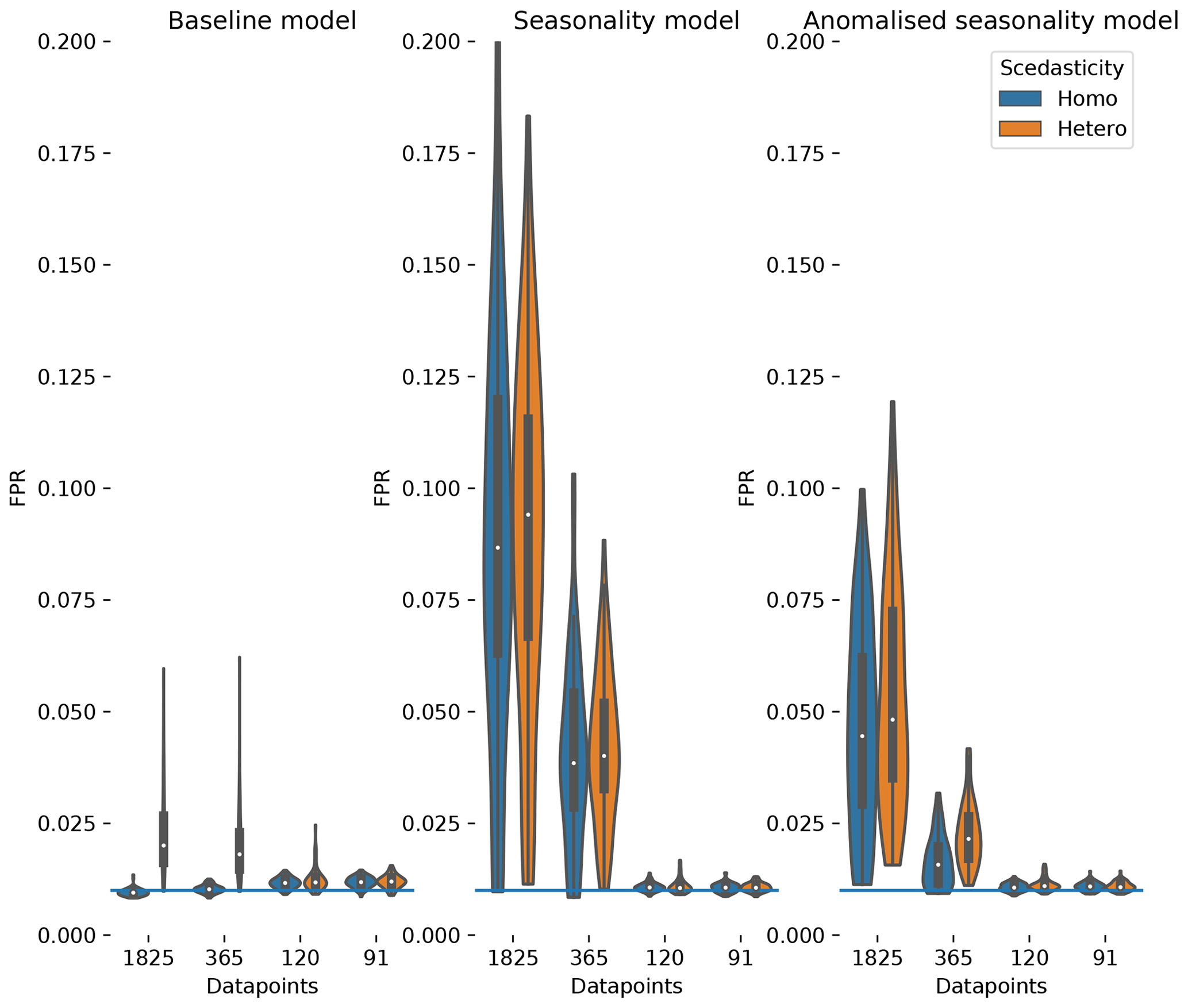
Figure 2The distribution of false positive detection rates estimated for the baseline dataset, the seasonality dataset and the anomalised seasonality dataset (mean seasonal cycle subtracted). The distributions are given for different time series length (number of datapoints). Additionally, the distributions are split to show the impact of heteroscedastic noise (orange) compared to normal distributed noise (blue). The significance level of 0.01 is given by a blue horizontal line.
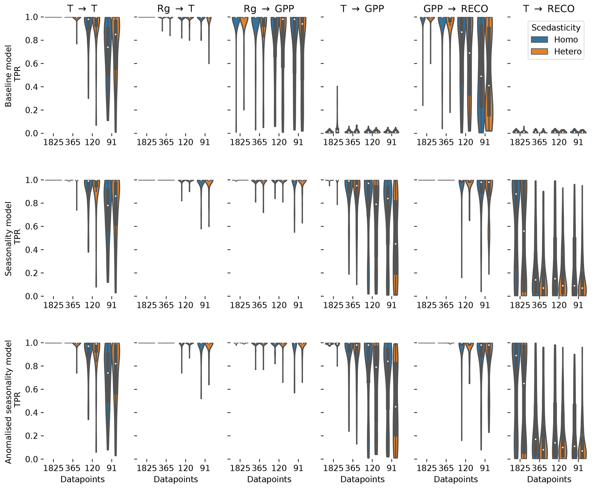
Figure 3The distribution of the true positive detection rates for each link in the test model estimated for the baseline dataset, the seasonality dataset, and the anomalised seasonality dataset. The distributions are given for different time series lengths (number of datapoints). Additionally, the distributions are split to show the impact of heteroscedastic noise (orange) compared to normally distributed noise (blue).
The FPR of homoscedastic time series in the baseline dataset is in the expected range of 0.01, the chosen significance level, indicating a well-calibrated test due to fulfilled assumptions. The assumption of stationarity is violated as soon as heteroscedasticity or seasonality is present. The effect on the FPR is an increase above 0.01 for time series length of 1 and 5 years, with a much stronger increase due to seasonality (factors of 4 and 8, respectively) than for heteroscedasticity (factor of 2).
The effect of non-stationarities on the TPR differs among the links. The detection of linear links (ℛg→𝒯 and 𝒯→𝒯) is not affected by seasonality and slightly improves for heteroscedastic dynamical noise. The detection of non-linear links is improved by seasonality, with the strongest effects in the link 𝒯→𝒢𝒫𝒫. The link 𝒯→ℛeco has a stronger non-linearity, and therefore the detection rate shows a weaker effect on seasonality. Furthermore, the coupling coefficient c5, the base of T, can be close to or be exactly 1 (see Fig. A3). This would actually cause, on the one hand, 𝒯→ℛeco to vanish, rendering a detection impossible and, on the other hand, result in a linear dependence of 𝒢𝒫𝒫 on ℛeco, which improves its detection. Heteroscedasticity seems to have a slight negative effect on non-linear links. In general, the TPRs in the seasonality dataset are quite high, even for non-linear links, and predominantly above 80 % and often reaching 100 %.
Comparing the TPRs of the non-linear links shows some disparity. The links 𝒯→𝒢𝒫𝒫 and 𝒯→ℛeco experience zero detection in the baseline dataset but partially considerable rates in the seasonality dataset with a strong dependence on the time series length. On the contrary, the median of the TPR of the links ℛg→𝒢𝒫𝒫 and 𝒢𝒫𝒫→ℛeco is above 95 % in the seasonality dataset, even for time series length as short as 91 d, but remains high in the baseline dataset. The removal of the seasonal cycle keeps the TPRs largely unaffected but reduces the FPR. Nevertheless, it still remains above the significance level by factors of 4 and 2 for 5-year and 1-year time series lengths, respectively.
In summary, the seasonality dataset exhibits high TPR even for non-linear links. Compared to stationary time series, the detection of non-linear links actually benefits from seasonality. The high detection, though, comes at the cost of a high false positive rate for time series length of and above 1 year. To a certain degree, the increase in FPR can be counteracted by anomalisation.
3.2 Majadas de Tiètar dataset
First, we look at the link consistency by comparing networks that were obtained for each tower within a month. The comparison is done for 2 months with strongly differing climate conditions: April and August. In Fig. 4 we compare the estimated link strengths (effect size estimated via partial correlation) as long as the corresponding links are significant in at least one network. The confidence intervals are overlapping for the majority of links, suggesting that the uncertainty of the fluxes is much smaller than the observed effects (El-Madany et al., 2018). Exceptions are found for only a few links (, , , , , , ; the number above the arrow indicates the lag) where the detection rates do not or barely overlap. Cross-links (a link from one variable to another) with two or more significant appearances are predominantly at zero lag. Approximately half of the links with lag 1 are auto-dependent links (a link from the past of a variable to its present). Comparing the links between the months of April and August, distinct differences can be noticed. First, August has slightly fewer significant links compared to April. Second, the only links remaining that are significant in two or three towers are between atmospheric variables. Third, the remaining link strengths tend to be weaker in August than in April.
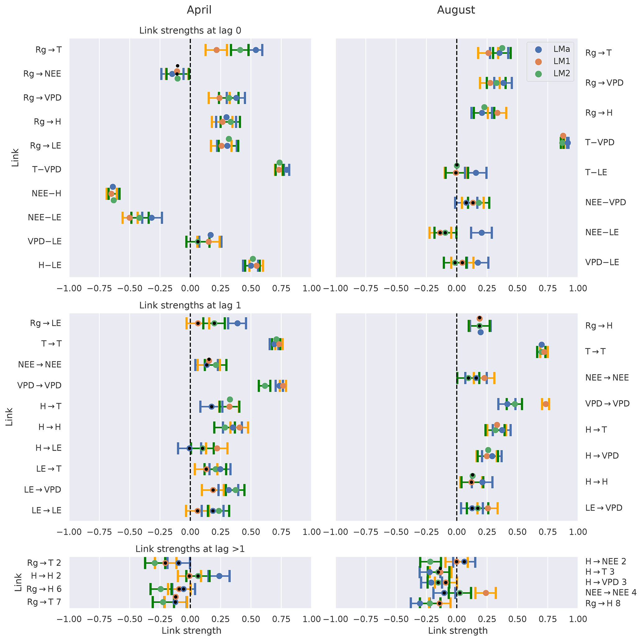
Figure 4Comparison of the networks of three eddy covariance measurement stations (LMa, LM1, LM2) located in Majadas de Tiètar (Spain). Links that are found to be significant in one of the three networks are included. For each link, the calculated strength of all three networks is plotted with its 90 % confidence interval. The colours blue, orange, and green correspond to the towers LMa, LM1, and LM2, respectively. The significance threshold is 0.01. If a link does not pass the significance, it is marked by a black dot. The links are grouped into lag 0 (top), lag 1 (middle), and all lags greater than 1 (bottom). Negative NEE is associated with carbon uptake by the ecosystem. Links at lag 0 are left undirected (–), yet as Rg is set as main driver, links incorporating Rg at lag 0 are directed (→).
The difference among the seasons is further investigated in Fig. 5, which shows process graphs for each month of the year. We combine the networks of the three towers to one process graph by plotting every link that is significant in at least one tower. The process graphs in Fig. 5 visualise clearly gradual changes within the interaction structure of the biosphere–atmosphere system during the course of a year. During the main growing season from February to May, NEE is coupled strongly to the energy fluxes latent (LE) and sensible heat (H). These connections weaken, disappear, or even switch sign during the dry season. Less regularly, NEE also shows connections to radiation (Rg) and temperature (T). Between the atmospheric variables, a basic network between VPD, T, Rg, and H remains intact and relatively constant in strength. The dominance of contemporaneous links is found as well, as already seen in Fig. 4. Aside from the decoupling of NEE from any variable in the dry period, there are additional interesting patterns. For example, the positive reappearance of the link between NEE and LE in September. Here, the onset of precipitation events (see Fig. A10) occurred, which led to strong respiration peaks (Ma et al., 2012). Creating such a network via lagged correlation would result in much more significant links (causing the network to be not interpretable as opposed to PCMCI) and NEE does not decouple from the atmosphere in August (see Fig. A7).
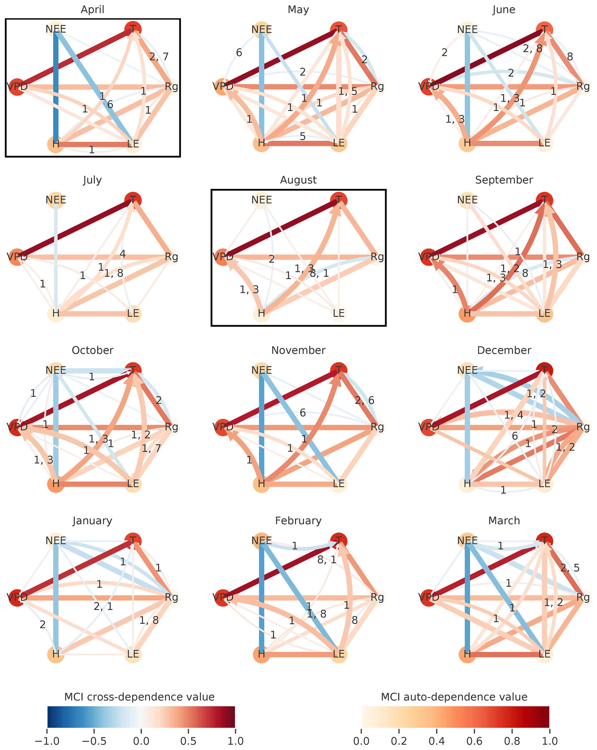
Figure 5To visualise the gradual changes in interaction structure the networks of the three towers are combined for each month. The number of significant occurrences of a link is given by its width. The link strength, given by the link colour, is calculated by averaging the significant links of the towers. The link's lag is shown in the centre of each arrow, sorted in descending order of link strength. The resulting graphs are shown for April 2014 until March 2015. The significance threshold is 0.01. The networks of April and August, illustrated in Fig. 4, are highlighted by a box.
The above results demonstrate that PCMCI is sensitive enough to capture seasonal differences and certain physiological reasonable biosphere behaviour. Moreover, PCMCI yields a better interpretable network structure than pure correlation approaches.
3.3 Gridded global dataset
The significant lags and MCI values of each climatic variable on NDVI were subject to inspection. In Fig. 6 the maximal MCI value and the corresponding lag are plotted for the links , with X being one of the climatic drivers: radiation, temperature, or precipitation. The chosen significance threshold was set to 0.05. Figure 7 shows the climatic driver with the largest MCI per grid point. PCMCI detects a regionally varying influence of climatic drivers. As expected, the boreal regions are strongly driven by temperature instantaneously, while (semi-)arid regions, which correspond predominantly to grass- or prairie-dominated areas, respond strongest to precipitation at a time lag of 1 month. Radiation is found to have a comparatively low spatial effect, with hotspots in southern and eastern China, central Russia, and eastern Canada.
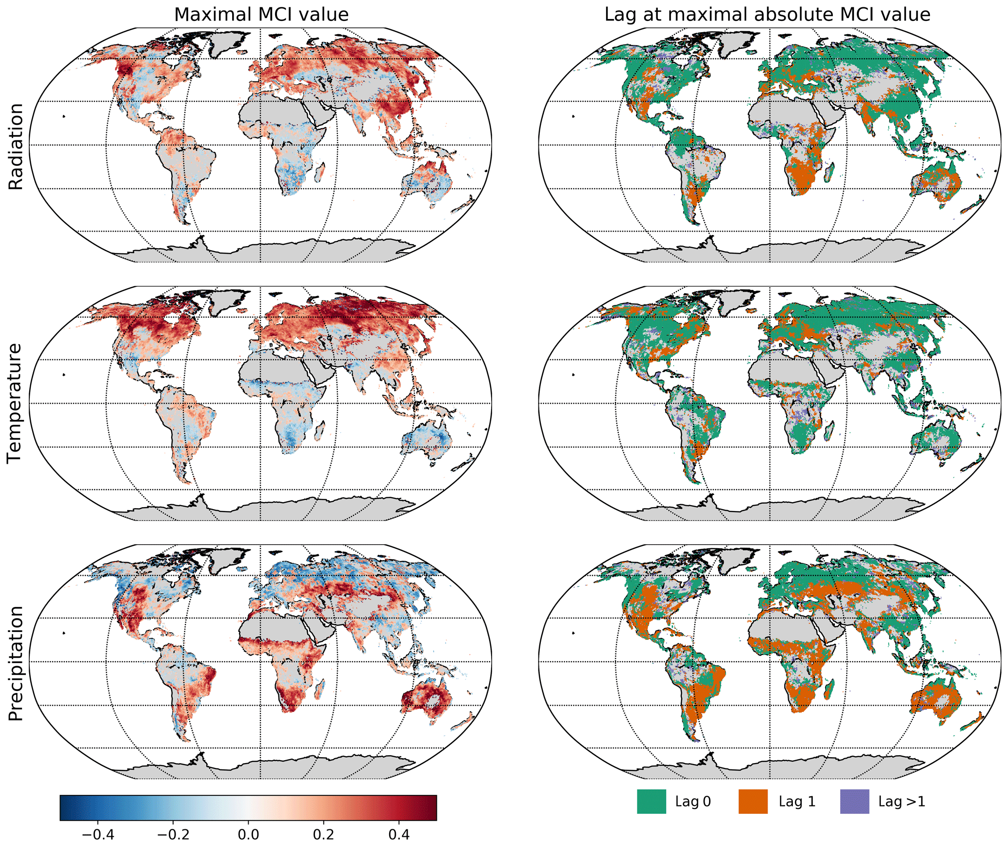
Figure 6Influence of climatic drivers on NDVI as calculated by PCMCI. The first column shows the estimated causal influence given as maximal absolute MCI value of climatic drivers on NDVI. The second column gives the time lag at which the maximal absolute MCI value occurs (in months).
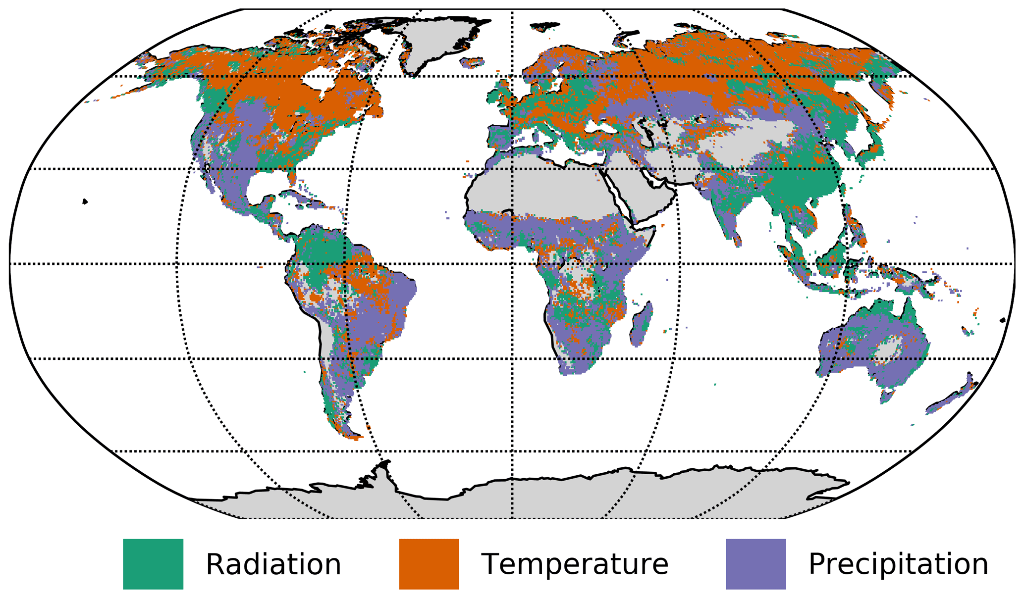
Figure 7Map of the strongest climatic driver (largest absolute MCI value) per grid point.
The dominant lags are found to be 0 and 1. Only a very small fraction of the total area shows a maximal MCI value at a higher lag of two or three months. The lags are also not equally distributed among the climatic drivers. Radiation and temperature are predominantly strongest at lag 0, while precipitation has a much larger fraction of area showing the strongest response at lag 1. Regions where the impact of Rg on NDVI is strongest at lag 1 tend to respond negatively to Rg but positively to precipitation at lag 1. On the other hand, a large part of the regions with the strongest impact of precipitation at lag 0 respond negatively to it but positively to radiation.
In summary, PCMCI estimates coherent interaction patterns that match well with anticipated behaviour based on vegetation type and prevailing climatic conditions.
Causal discovery methods promise an improved understanding and can help to come up with new hypotheses about the interaction between biosphere and atmosphere (Christiansen and Peters, 2020; Runge et al., 2019a). However, the underlying assumptions need to be properly taken into account. The coupled biosphere–atmosphere system possesses several challenges that potentially violate the underlying assumptions of causal discovery in general and the employed method's assumptions in particular. Here, we investigate the effect of a violation of assumptions on PCMCI network estimates.
With regard to expected non-linearities in biosphere–atmosphere interactions, using a linear independence test within the PCMCI framework may not be adequate. We justify our choice with the following arguments: first, non-linearities are often approximated linearly. Second, a linear regression based test has a much higher power for detecting linear links than a non-parametric test (Runge, 2018) and can hence already detect links at smaller sample sizes. Third, linear partial correlation is easily interpretable, for example, positive and negative MCI values. This motivation is supported on the one hand by the results of the test model and on the other hand by additionally performed analyses on the observational datasets using Gaussian regression and distance correlation as an independence test. These results (see Figs. A8, A9, A11) show similar patterns, but due to the low sample sizes exhibit lower statistical significance. In general, the derived results show a high detection power with a strong consistency in calculated effect strengths on eddy covariance data and global, regularly gridded reanalysis data that leads to easily interpretable patterns. Observed drawbacks are a high FPR in cases of violated assumptions, especially strong periodicity, as well as the appearance of contemporaneous lags in measurement datasets.
4.1 Lessons learned from the test model
The probability of detecting a link with PCMCI depends strongly on a link's MCI effect size, which is larger for strong variance in the driver and a low variance in the receiver (see Sect. 2.5). Several results can be explained by this observation. First, the variance of three out of five drivers of cross dependencies in the test model are either directly or indirectly (via 𝒢𝒫𝒫) influenced by ℛg, which has the highest variance of all variables. Consequently, the detection power of the three links is large, almost 100 %. In comparison, the other variables' variances are weaker, since they are influenced by 𝒯, which results in a lower detection power. This is the origin of the disparity in detection rates of the non-linear links. Second, the partially strong increase in TPR of non-linear links (influenced in a multiplicative way by 𝒯) from the baseline dataset to the seasonality dataset can also be explained by this increase in variance. A multiplicative link is actually not generally expected to be found by ParCorr (Runge, 2018), but the value of the multiplicative factor is dominated by the seasonal value, and not the dynamical noise, which might cause a scaling of the dynamical noise terms rather than a random distortion. Third, the dependence on the variance ratio can also explain the difference in TPR between homoscedastic (equal error variance) and heteroscedastic (error variance changing over time) time series, i.e. the variance of ℛg and 𝒢𝒫𝒫 exhibits a strong seasonality, with its peak in summer, while the variance of 𝒯 is rather constant. This explains, for example, the strong decrease in TPR for the link 𝒯→𝒢𝒫𝒫 at 91 d time series length when comparing homoscedasticity to heteroscedasticity. The decrease in TPR is less pronounced when another season, implying a different variance, is chosen for this comparison. As links with weak driver variance and strong response variance are more likely to be missed, one may ask what effect this will have on the detection of feedback loops where one variable has low and the other high variance. Here lies a limitation of the test model where no feedback loops were implemented.
Seasonality and heteroscedasticity constitute violations of the stationarity assumption underlying the independence test ParCorr. Seasonality constitutes a common driver in this model. In general, such common drivers increase the dependence among the variables and hence lead to a higher detection rate for true links (TPR) as well as a higher false positive rate (FPR) for absent links if this driver is not conditioned out properly. This additionally causes the TPR and the FPR rate to increase in the seasonality model. As shown in Runge (2018), including the cause of the non-stationarity as an exogenous driver in the analysis allows PCMCI to regress out its influence on the other variables. However, for ParCorr this is only valid if the dependence on the non-stationary driver is linear. Therefore, the regression on ℛg fails for 𝒢𝒫𝒫 and ℛeco in the test model. With this ill-posed setting, the probability to detect false links increases with increasing time series length or when more periods are included. Stationarity in the mean is obviously also not fully guaranteed when subtracting the seasonal mean. Here we observe that the FPR stays above the significance level for the anomalised seasonality dataset. One can ask whether the FPR stays above the significance threshold because subtracting the seasonal mean does not remove the heteroscedasticity. However, we attribute this high FPR to a not fully removed seasonality since the FPR of both homoscedastic and heteroscedastic time series decreases by roughly the same amount in the anomalised seasonality dataset and the effect of heteroscedasticity is rather weak in the baseline dataset. The increasing FPR with increasing time series length can further raise doubts regarding the analysis of long time series. For such an analysis, though, the assumption of causal stationarity should first be assessed. For example, the link from radiation to GPP vanishes in winter as there is mostly no active plant material left. To account for causal stationarity, the analysis should be limited to time series sections where the causal structure is expected to be similar. This is typically done by limiting the analysis to a specific time period (i.e. “masking”), e.g. a specific season, month, or time of the day. Such masking additionally further reduces influences of remaining seasonality or heteroscedasticity. One can argue, as in Peters et al. (2017), that the causality of a system is invariant even between seasons because the physical mechanism is the same in all seasons. Yet, while the physical, i.e. functional relationship might be constant over time, its imprint in the time series might vary. For example, a functional dependence f(x) might be “flat” for small values of x and linearly increasing for larger values. If only small values occur in the winter season, then the link is absent, while it “appears” only in the summer season. Across all seasons, this can be considered a non-linear functional dependence f(x). In practice, restricting an analysis to different seasons can help in interpreting the mechanism and is performed here using a linear framework.
Summarising the results of the test model, the different detection rates, disparity among non-linear links, and the detection of multiplicative links are largely explainable via the effect of the variance on the link detection. Yet, the discussion revealed the need for further research in several aspects. On the one hand, feedback loops are not included in the test model yet are an important aspect in natural systems. On the other hand, removing non-stationarities is essential to keep the false positive rate in the expected range, but standard procedures of subtracting the mean seasonal cycle are not sufficient. Further, the effect of non-stationarity on the causal network structure needs to be investigated.
4.2 Causal interpretation of estimated networks from observational data
In both the half-hourly time-resolved eddy covariance data and the monthly global dataset, the predominant type of dependence found is contemporaneous. PCMCI leaves these undirected since no time order indicating the flow of causal information is available. Further, as discussed in Sect. 2.2, contemporaneous common drivers or mediators are not accounted for. The consequence is that both spurious contemporaneous and spurious lagged links can appear if they are due to contemporaneous variables. For interactions that are contemporaneous in nature, since they occur on considerably shorter timescales than the time resolution, PCMCI is not the optimal choice regarding a causal interpretation and other methods should be applied in conjunction (Runge et al., 2019a). Further, we faced a trade-off between fulfilling causal assumptions and detection power. In practice, accounting for causal stationarity (by limiting the analysis to certain periods of the dataset) means decreasing the number of available data points but accounting for causal sufficiency leads to an increase in dimensionality by adding variables and increasing the maximal lag. Both will lead to a decrease in detection power, which can affect the network structure. PCMCI alleviates the curse of dimensionality by applying a condition selection step, but one still cannot indefinitely add more variables. Another important factor that affects detection power and dimensionality is the time resolution. There are several points in favour and against increasing time resolution. On the one hand, increasing time resolution can resolve contemporaneous links and potentially increases the detection power due to an increased number of datapoints. On the other hand, the dimensionality increases if the maximal lag is adapted. Further, causal information might be split apart and distributed over more lags, rendering the links at each individual lag less detectable. This can cause links to disappear, but links can also appear if new processes are resolved at a higher timescale. Finally, observational noise (measurement errors) might be larger in higher-resolution data than in aggregated data, as it is averaged out in the latter and thus affects link detection less. Consequently, when comparing network structures based on different settings, i.e. maximal lag, included variables, time resolution, and considered time period, the (dis)appearance of single links among specific variables can stem from several factors, i.e. a change in detection power, a changed (conditional) dependency, or due to a common driver. These factors together with a non-zero false positive detection rate are challenging for a causal interpretation. Therefore, detected links should be interpreted with care and can give rise to new hypotheses and analyses involving further variables. Generally, a causal interpretation is more robust regarding the absence of links (see Sect. 2.2). Specifically, it does not require that all common drivers are observed.
Nevertheless, robust patterns were identified in our studies that are also consistent with other studies. Furthermore, a causal analysis has the advantage of an enhanced interpretability compared to correlative approaches. First of all, we could show that the networks' estimated link strengths are consistent for observational data, even though measurement error affects the data. The dataset used was suitable for this analysis, as the measurement stations are located in a reasonably homogeneous ecosystem that shows only little spatial variation (El-Madany et al., 2018). Thus, also the interaction between biosphere and atmosphere is expected to change only marginally across space within this ecosystem. Second, the gradual changes in plant activity that are taking place in the ecosystem of Majadas de Tiètar throughout the year do emerge very well in the coupling strength of daytime NEE to the atmospheric variables. The observed decoupling during the dry season is in accordance with the one of a soybean field during drought conditions observed by Ruddell and Kumar (2009). The gradual changes in ecosystem activity are not visible in a pure (lagged) correlation analysis or are only visible in colour or density changes but the large number of significant links prevents any detailed interpretation on the physical mechanisms and changes thereof. The large number of significant links compared to the PCMCI networks stems solely from the absence of conditioning in common drivers or mediating variables, which often leads to an overestimation of the link strength in correlation networks. As a result, processes, such as the decoupling of NEE during the dry period, stay hidden. To reduce the effect of confounding, analyses often utilise partial correlation (see, e.g. Buermann et al., 2018). However, a partial correlation can introduce new dependencies (as opposed to removing them) if one conditions on causal effects of the variables under consideration (the “marrying parents” effect). This issue is avoided in PCMCI by only conditioning on past variables. Additionally, PCMCI chooses only relevant variables as conditions by applying the PC condition selection step, which is especially valuable in high-dimensional study cases and improves detection power and computation time (Runge, 2018).
The global study of climatic drivers of vegetation shows a general pattern of lags and dependence strengths of vegetation on climatic variables that is easily interpretable. The boreal regions appear energy limited and especially driven by temperature (see Fig. 6c), while the strongest dependence of (semi-)arid regions on precipitation reflects their limitation in water supply. Two recent studies performed a similar analysis. Both Wu et al. (2015) and Papagiannopoulou et al. (2017b) investigated lagged effects and dependence strengths of NDVI on precipitation, temperature, and radiation. Wu et al. (2015) estimated the lags of the strongest effects via an univariate regression of the climatic drivers on NDVI and subsequently used those lags to fit a multivariate regression model of the climatic drivers on NDVI and determined their relative effects. Papagiannopoulou et al. (2017b) applied a non-linear Granger causality framework utilising a random forest predictive model; the method was presented by Papagiannopoulou et al. (2017a). We recognise that similar patterns are observed in Wu et al. (2015), but the lags at the maximal MCI value are usually lower than the one found in Wu et al. (2015), which stems from the methodical differences. Besides having used anomaly values, PCMCI regresses both NDVI and the climatic drivers on their parents before calculating the MCI value (see Sect. 2.5). This especially removes the influence of autocorrelation. Runge et al. (2014) shows how autocorrelation affects the correlative lag causing it to be larger for stronger autocorrelation; thereby, the correlative lag may become larger than the causal lag. Therefore, according to Fig. 6b, the causal information embedded in monthly resolution is predominantly received within 1 month. Finding the strongest causal links at a time lag up to 1 month appear in agreement with Papagiannopoulou et al. (2017b). Additionally, the spatial distribution of the strongest climatic influences compares well, but there are certain noteworthy differences that do not necessarily stem from masking differences, i.e. that we took only values belonging to the growing season while Papagiannopoulou et al. (2017b) took the whole time series. First, there is little significant Granger causality of water availability found in boreal regions while there are significant negative causal dependencies detected via PCMCI. Second, NDVI in arid regions is not (or is only partially) Granger caused by radiation and temperature but in part shows a negative PCMCI value for those variables. There might be physiological reasons that can explain the PCMCI patterns, i.e. waterlogging or temperatures that are too high. To explain the differences though, we could identify two possible reasons. First, Papagiannopoulou et al. (2017b) masked out negative influences of radiation, arguing that radiation is not negatively affecting NDVI. They found that negative influences of Rg are usually a consequence of poor conditioning on other variables. Second, a precipitation event in boreal regions coincides with a reduction in radiation and temperature. Boreal regions usually do not suffer from water shortages. Thus, they respond more strongly to the reduction of radiation and temperature than precipitation. As precipitation is coupled negatively to radiation and temperature at lag 0, the effect of precipitation on NDVI is found to be negative. Thus, the link might be an effect of the contemporaneous common driver scheme and therefore would not be causal. In fact, a similar argumentation can be given for the negative impact of temperature and radiation on NDVI in arid regions.
In summary, we pointed out the need for careful interpretations in applying causal discovery methods and especially highlighted the challenges linked to the study of biosphere–atmosphere interaction via PCMCI. We demonstrated that the network structures estimated from observational data are explainable with respect to plant physiology and climatic effects. Finally, our study shows that causal methods can deliver better interpretability and a much improved process understanding in comparison to correlation and bivariate Granger causality analyses that are ambiguous to interpret since they do not account for common drivers.
4.3 Outlook
The preceding discussion has shed light on the merits of PCMCI, as well as the challenges of applying causal discovery methods. Runge et al. (2019a) discuss further challenges and methods and give an outlook of how multiple methods can be combined to alleviate limitations.
Here we tested PCMCI, an algorithm that estimates causal graphs from empirical time series. We specifically explored two types of datasets that are highly relevant in biogeosciences: eddy covariance measurements of land–atmosphere fluxes and global satellite remote sensing of vegetation greenness. The causal graphs estimated from the eddy covariance data collected in a Mediterranean site confirm patterns we would expect in these ecosystems: during the dry season's plants senescence, for instance, the ecosystem's carbon cycle (NEE) decouples from meteorological variability. On the contrary, during the main growing season, with warm and humid conditions, strong links between NEE, LE and H characterise the graph. Using the causal framework, not only the strongly contrasting states emerge in the graph structure but also the gradual transitions that relate to minor changes like the connectivity of sensible heat to temperature with progressing dryness. A purely correlative analysis, instead, is not able to resolve these patterns. PCMCI allows us to identify and focus on fewer (only those that are highly relevant) dependencies. Applying the approach to three replicated eddy covariance systems shows the robustness of the method to random errors in the fluxes measurements and confirms one of the assumptions of eddy covariance: above a relatively homogeneous terrain the fluxes measured should be spatially invariant as should the underlying causal relationship between climate and fluxes. The global analysis of NDVI in relation to climatic drivers confirms the known patterns of dependence strengths of vegetation on climatic variables: boreal regions are energy limited and especially driven by temperature and secondarily by radiation, while in semi-arid regions vegetation dynamics are strongly dependent on water supply. However, obtained response times of vegetation to climatic variations are lower using PCMCI than correlation which can be attributed to a better treatment of the autocorrelation in the time series and cross-relations among climate variables. Compared to merely correlative approaches, this leads to a interpretable pattern of driver–response relationships. In short, the new developments achieved in causal inference allow us to gain well-constrained insights on processes that would otherwise be drowning in the correlation chaos. Therefore, we hope that this study fosters usage of causal inference in analysing interactions and feedbacks of the biosphere–atmosphere system and furthermore exhibits our demand of further developments.
Table A1PCMCI parameters that were used differently from default settings.
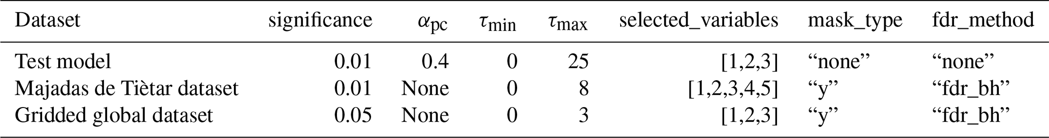
Table A2List of FLUXNET sites used for the generation of artificial datasets and the time period used.

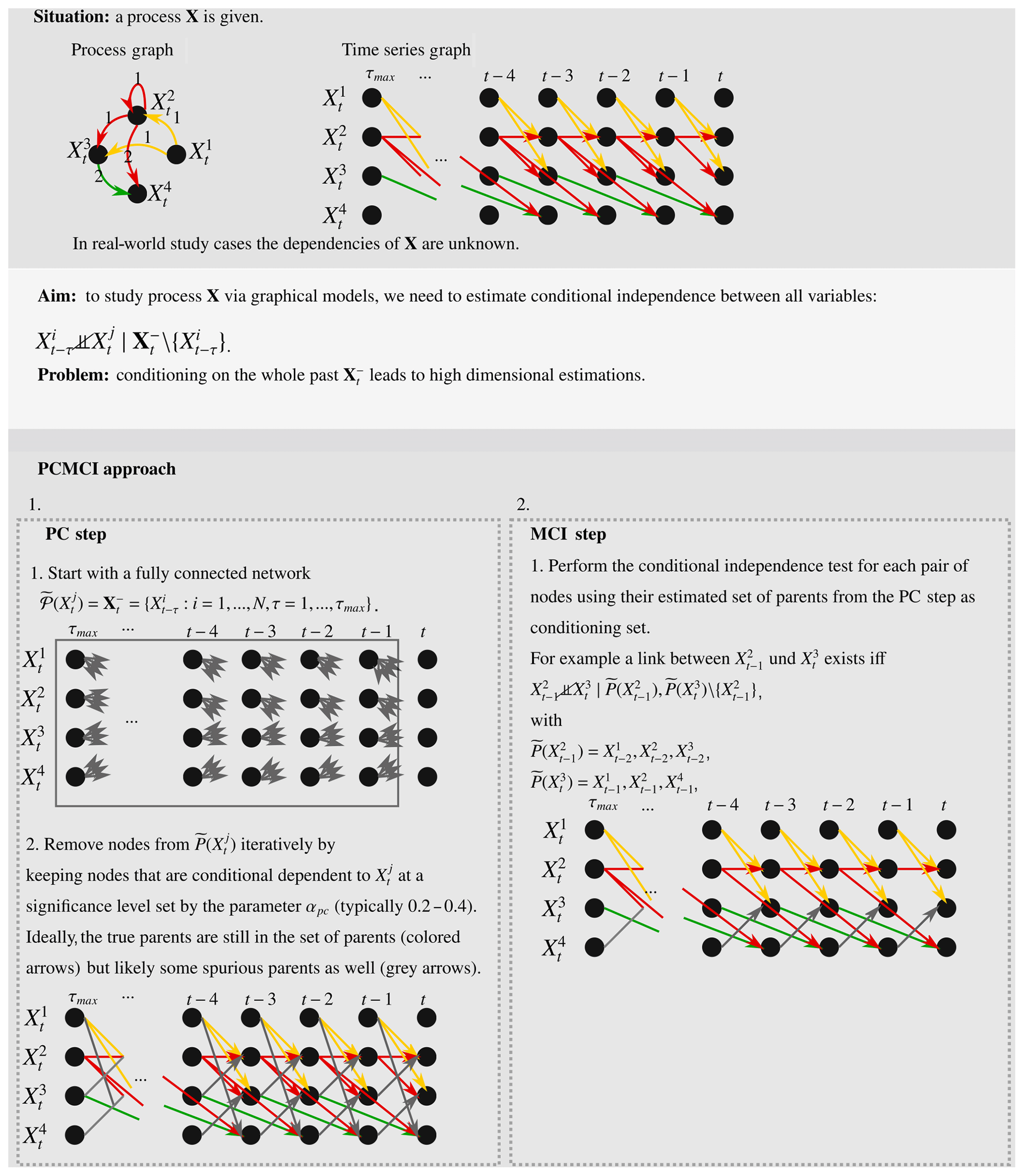
Scheme A1Schematic overview of the aim and approach of PCMCI using time series graphs as a visualisation tool.
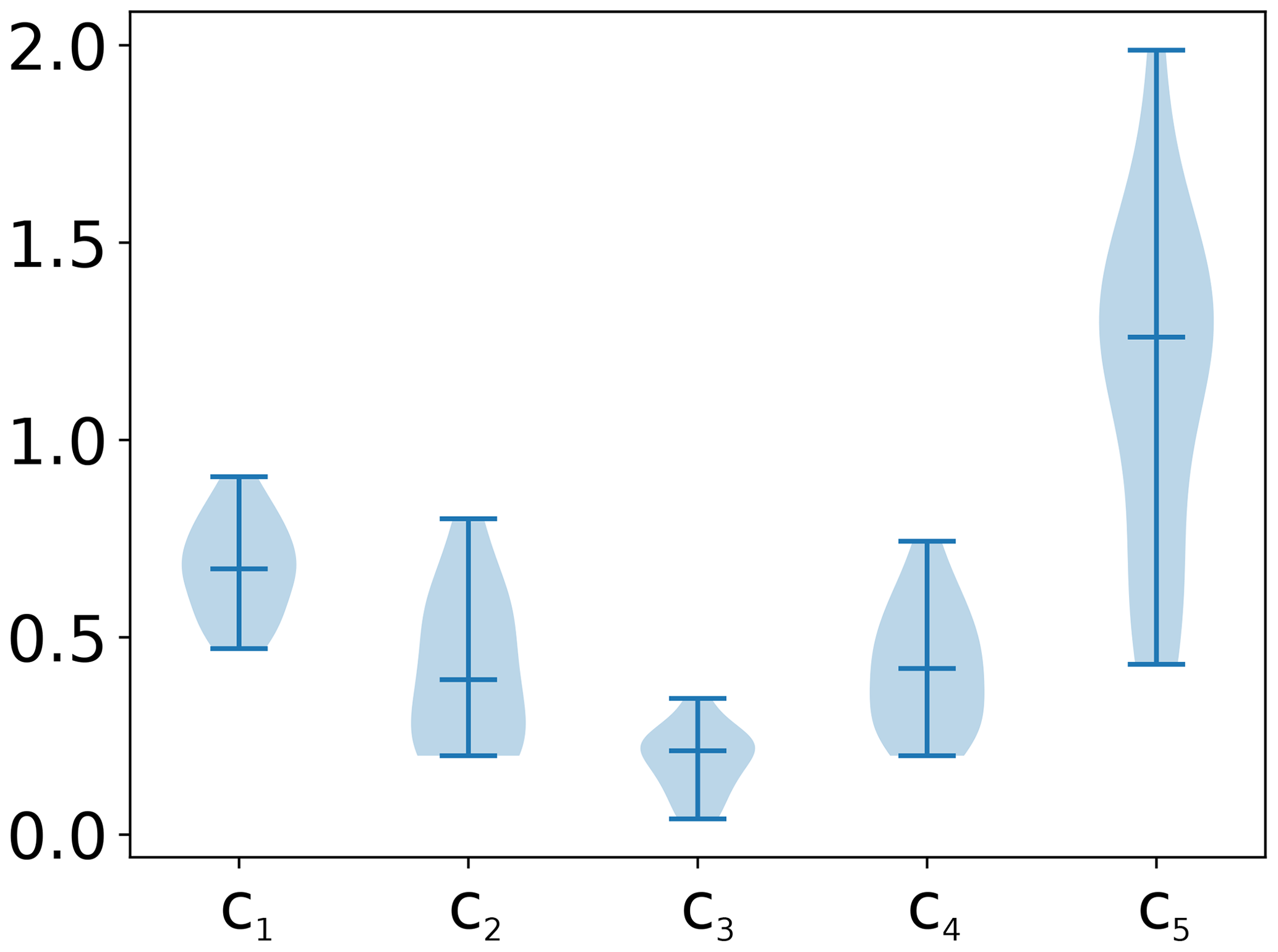
Figure A1Distribution of coupling coefficients obtained after fitting the test model to the Fluxnet sites. Shown here are the distributions used for generation of heteroscedastic time series.
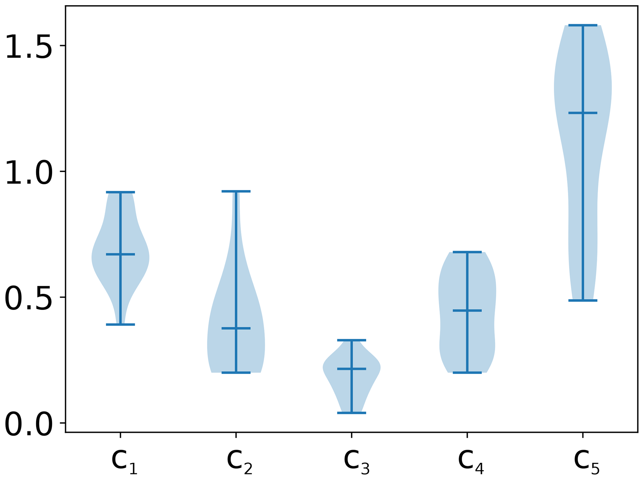
Figure A2Distribution of coupling coefficients obtained after fitting the test model to the Fluxnet sites. Shown here are the distributions used for generation of homoscedastic time series.

Figure A3Distribution of time lags obtained after fitting the test model to the Fluxnet sites. Shown here are the distributions used for generation of heteroscedastic time series.
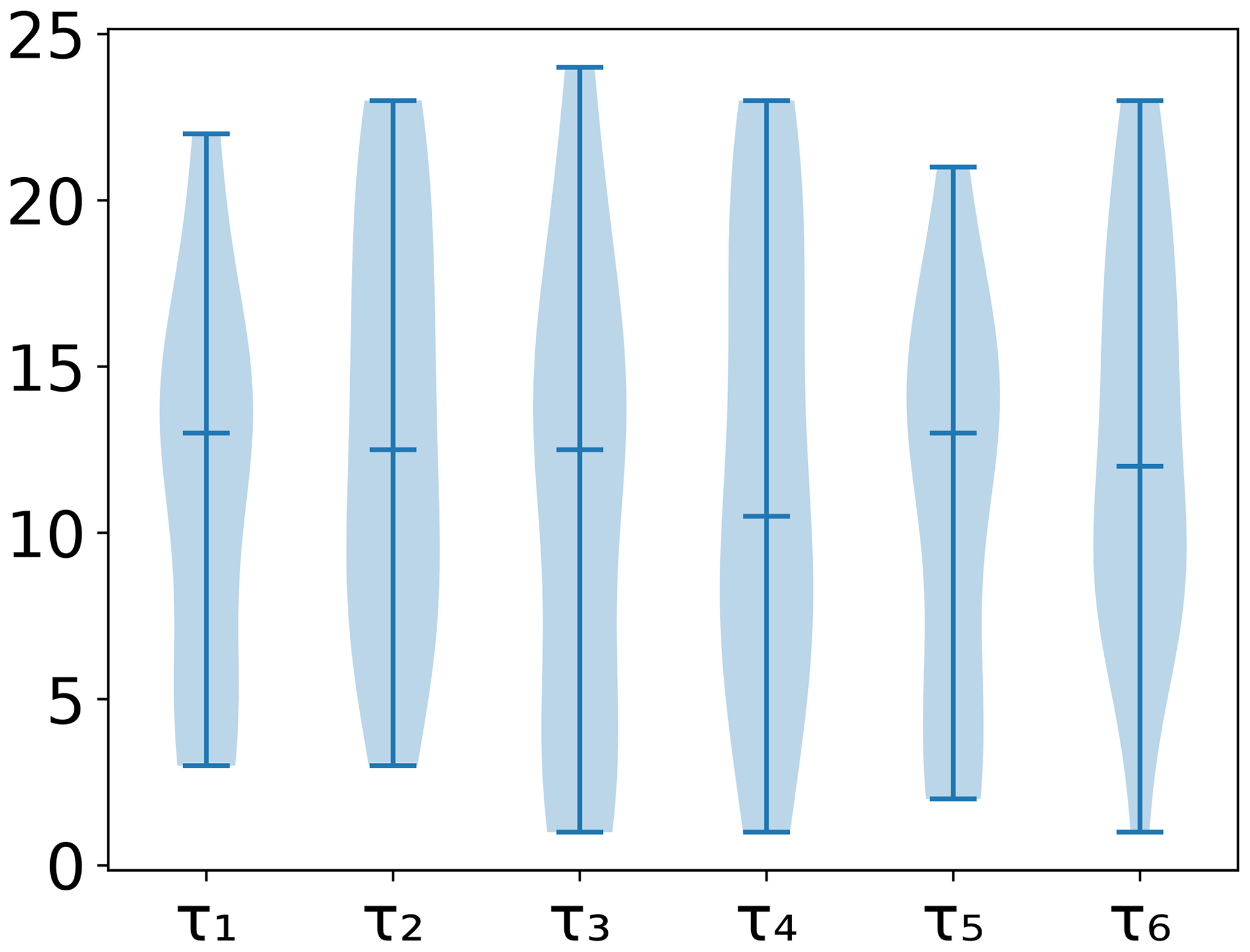
Figure A4Distribution of time lags obtained after fitting the test model to the Fluxnet sites. Shown here are the distributions used for generation of homoscedastic time series.
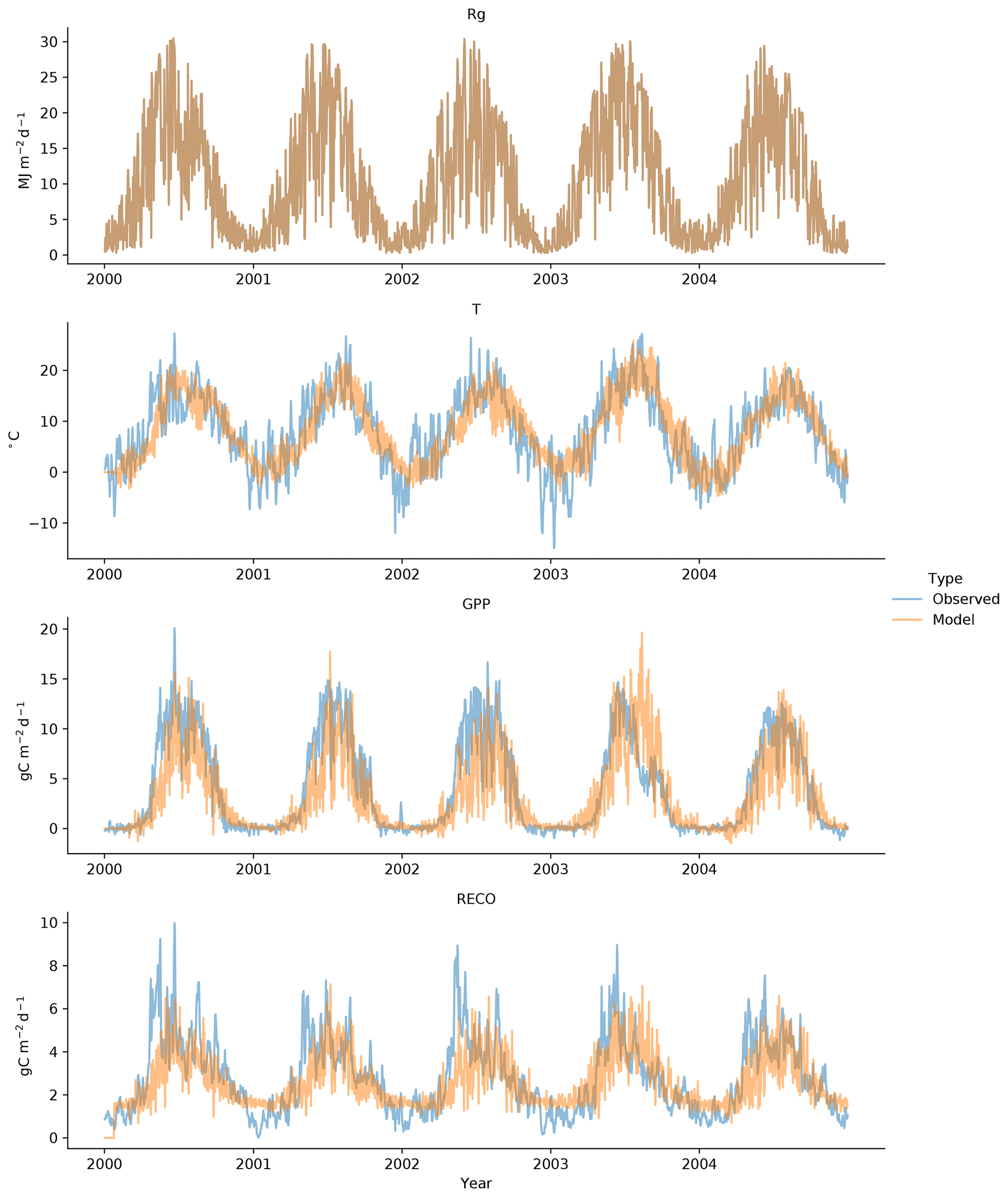
Figure A5Observed (blue) and test model (orange) time series for the Hainich Fluxnet site. The model data were produced with heteroscedastic noise.
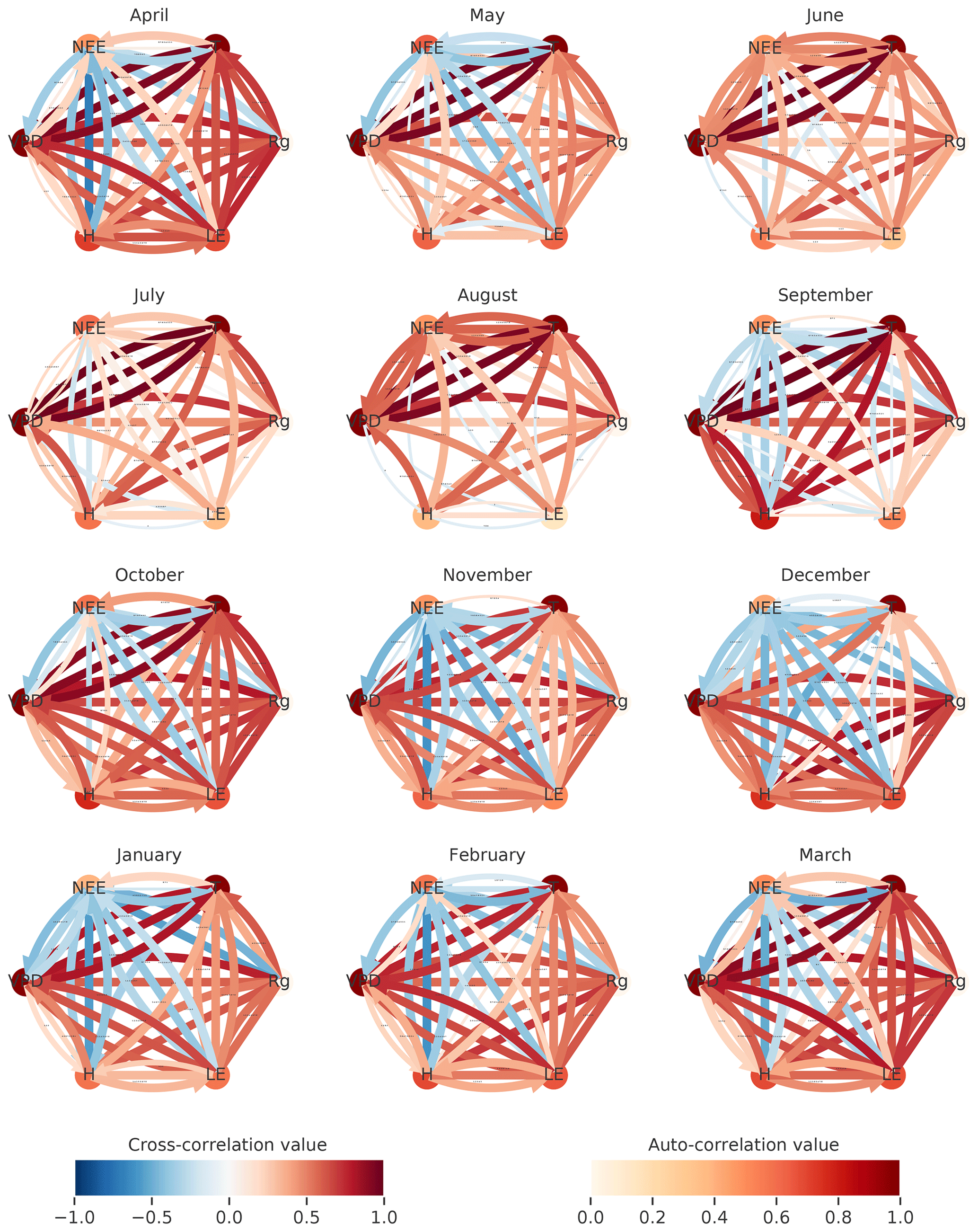
Figure A6The same as Fig. 5 but using simple correlation analysis to estimate the graph structures. The number of significant occurrences of a link is given by its width. The link strength, given by the link colour, is calculated by averaging the significant links of the towers. Link labels indicating the lag were removed to improve link visibility. They typically ranged from 1 to 8 (full range of possible lags). The resulting graphs are shown for April 2014 until March 2015. The significance threshold is 0.01.
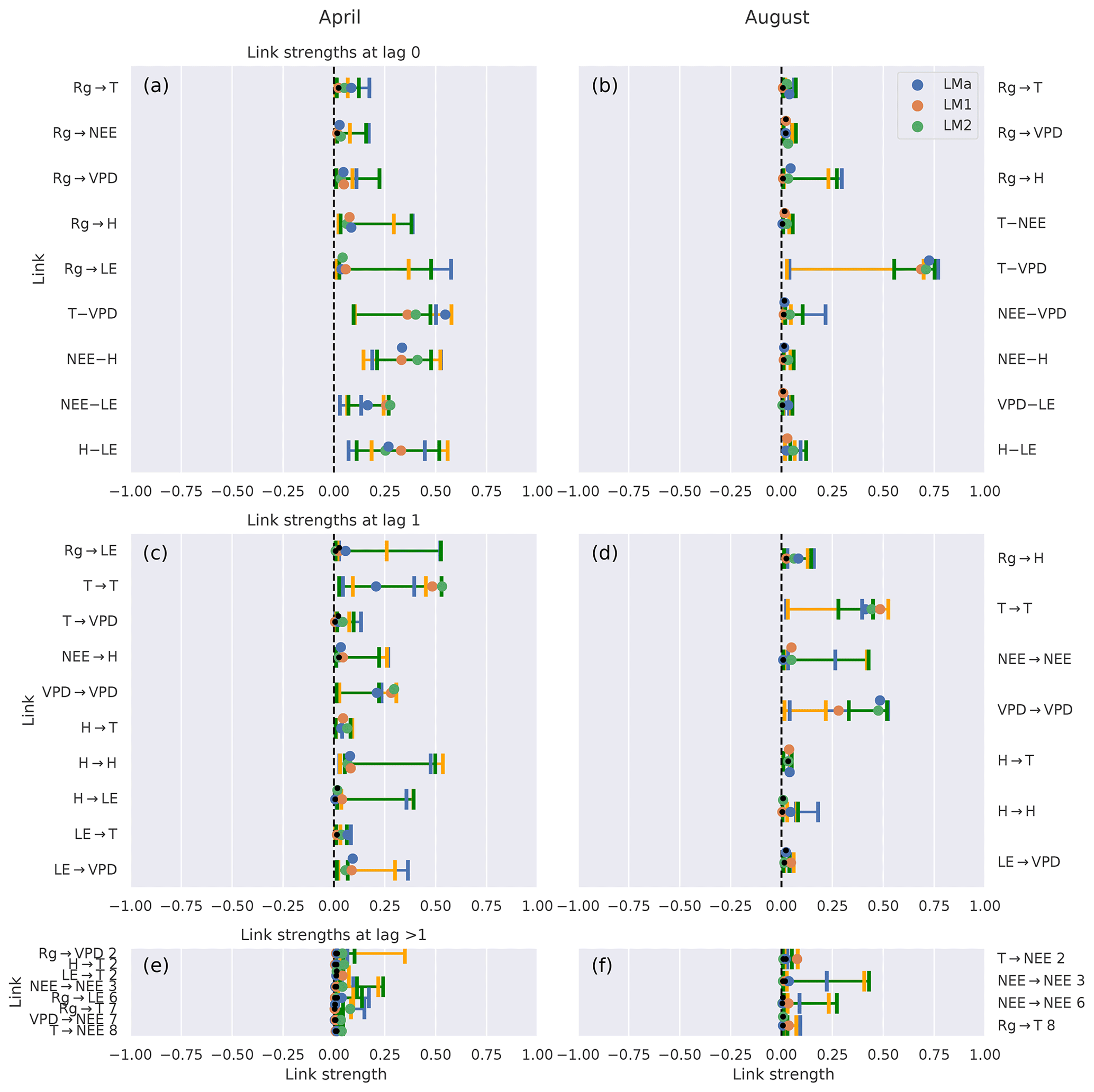
Figure A7The same as Fig. 4, but the analysis was performed using a non-linear independence test. Comparison of the networks of three eddy covariance measurement stations (LMa, LM1, LM2) located in Majadas de Tiètar (Spain). Links that are found to be significant in one of the three networks are included. For each link, the calculated strength of all three networks is plotted with its 90 % confidence interval. The colours blue, orange, and green correspond to the towers LMa, LM1, and LM2, respectively. The significance threshold is 0.01. If a link does not pass the significance, it is marked by a black dot. The links are grouped into lag 0 (a, b), lag 1 (c, d) and all lags greater than 1 (e, f). Links at lag 0 are left undirected (−), yet as Rg is set as main driver, links incorporating Rg at lag 0 are directed (→). Note that Gaussian process regression and distance correlation (GPDC) only yields positive link strengths. Further, the strength values estimated with GPDC are rather weak due to the low number of datapoints and the larger sensitivity of that method to the sample size.
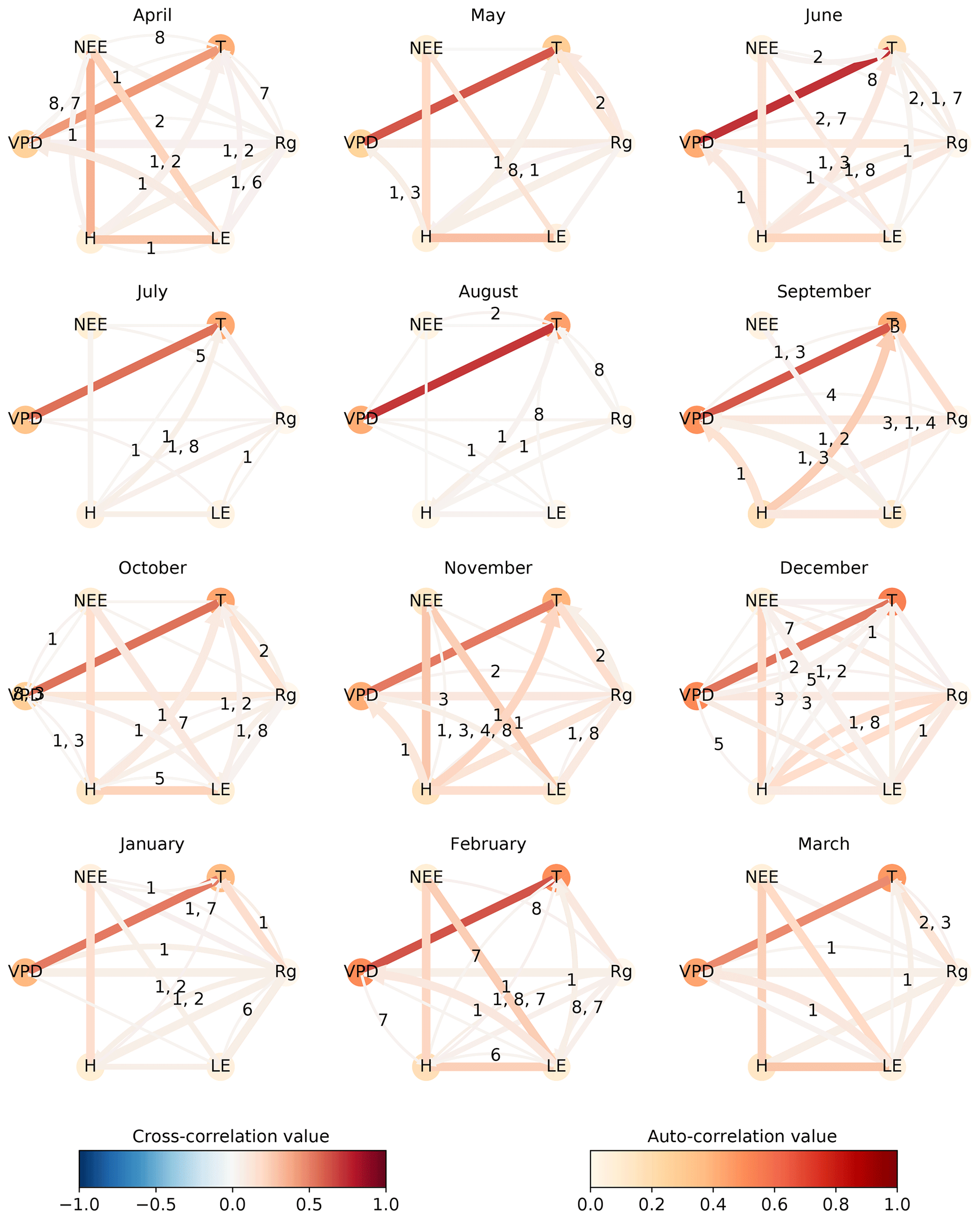
Figure A8The same as Fig. 5, but the analysis was performed using a non-linear independence test. The number of significant occurrences of a link is given by its width. The link strength, given by the link colour, is calculated by averaging the significant links of the towers. The link's lag is shown in the centre of each arrow, sorted in descending order of link strength. The resulting graphs are shown for April 2014 till March 2015. The significance threshold is 0.01. Note that GPDC only yields positive link strengths. Further, the strength values estimated with GPDC are rather weak due to the low number of datapoints and the larger sensitivity of that method to the sample size
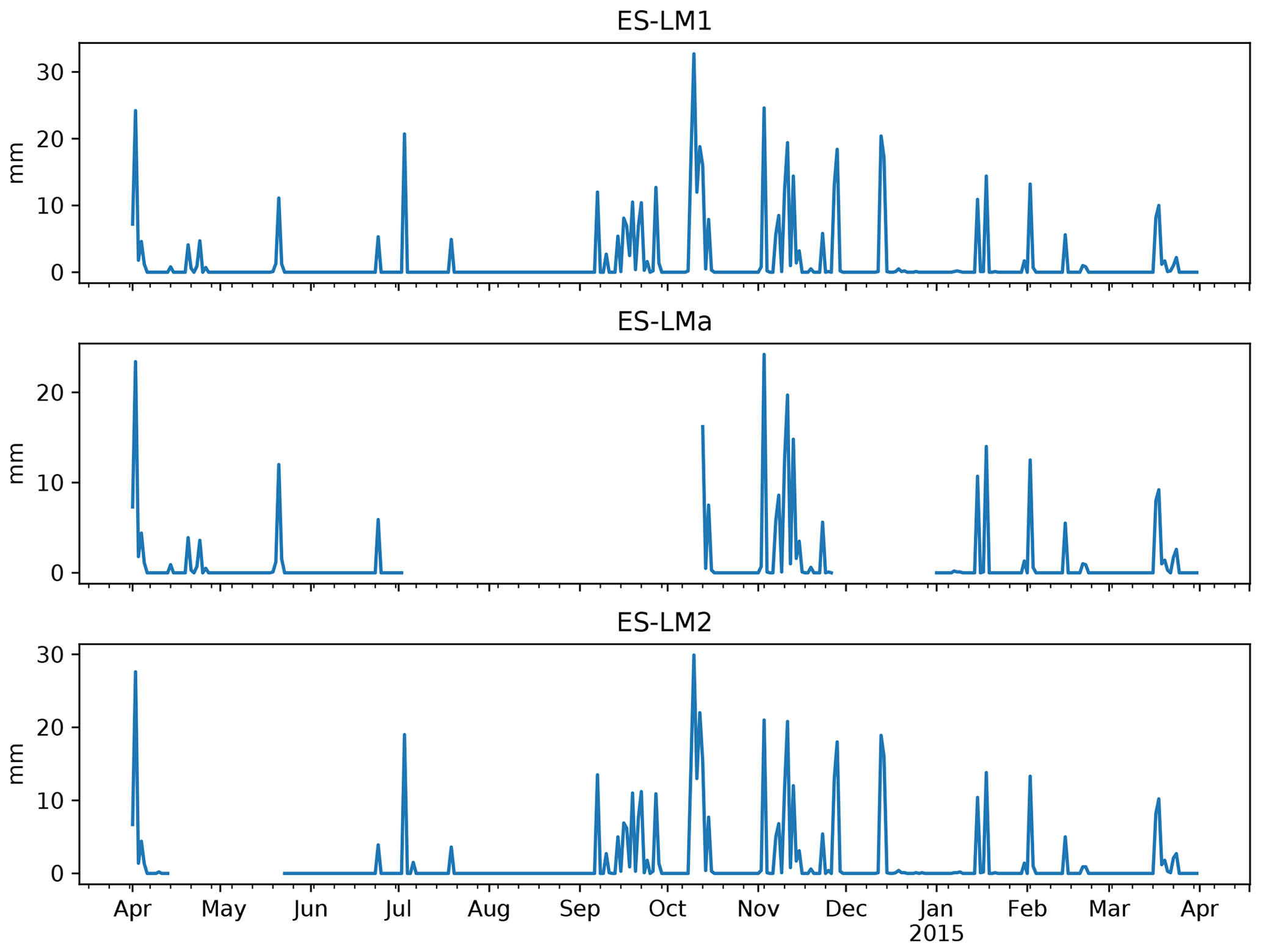
Figure A9Daily aggregated precipitation in Majadas de Tiètar measured at the three tower sites from April 2014 to March 2015. Missing values are plotted as gaps.
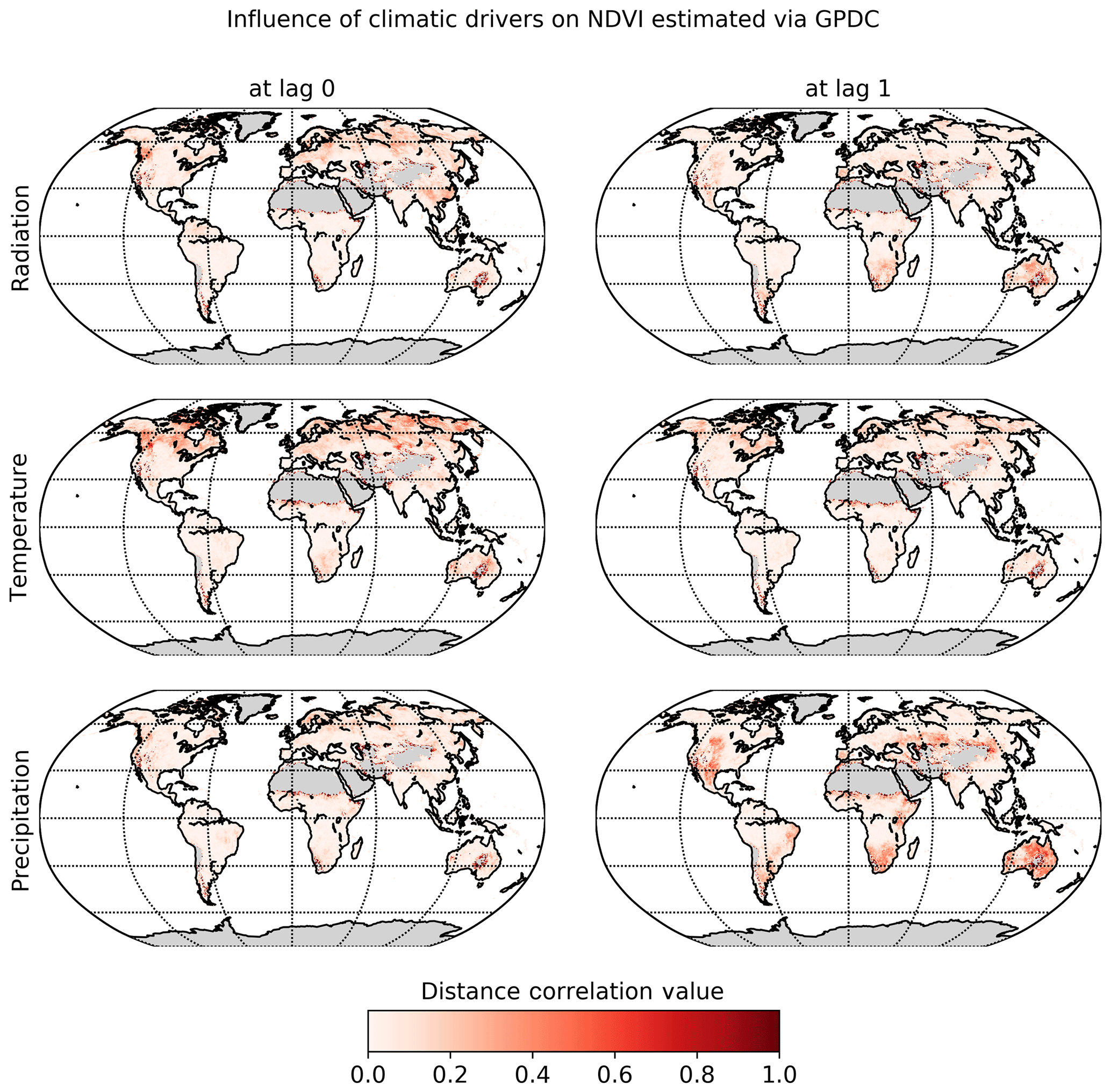
Figure A10Influence of climatic drivers on NDVI as calculated by PCMCI in conjunction with the non-linear independence test GPDC (similar to Fig. 6). The first and second columns show the estimated causal influences of climatic drivers on NDVI at lag 0 and 1, respectively.
The eddy covariance data of the FLUXNET sites can be downloaded from the official web page (https://fluxnet.fluxdata.org/, last access: 14 June 2018). For further information, please see Table A2.
CRU temperature and precipitation data are available at http://catalogue.ceda.ac.uk/uuid/3f8944800cc48e1cbc29a5ee12d8542d (University of East Anglia Climatic Research Unit et al., 2008).
CRUNCEP radiation data can be downloaded via ftp://nacp.ornl.gov/synthesis/2009/frescati/temp/land_use_change/original/readme.htm (Viovy, 2016).
The NDVI dataset is available at https://ecocast.arc.nasa.gov/data/pub/gimms/3g.v1/ (Pinzon and Tucker, 2014).
The TIGRAMITE software package that includes PCMCI can be found on github https://github.com/jakobrunge/tigramite/ (Runge, 2017). All other code will be made available upon request.
CK and MDM designed the study with contributions from JR and DGM. CK conducted the analysis and wrote the manuscript. All authors helped to improve the manuscript. AC, MM, TEM, and OPP conducted field experiments in Majadas de Tiètar, processed and provided its data, and helped with their interpretation.
The authors declare that they have no conflict of interest.
We thank Maha Shadaydeh, Rune Christiansen, Jonas Peters, Milan Flach and Markus Reichstein for useful comments. Christopher Krich thanks the Max Planck Research School for global Biogeochemical Cycles for supporting his PhD project. The authors affiliated with the Max Planck Institute for Biogeochemistry thank the European Space Agency for funding the “Earth System Data Lab” project.
This work used eddy covariance data acquired and shared by the FLUXNET community, including these networks: AmeriFlux, AfriFlux, AsiaFlux, CarboAfrica, CarboEuropeIP, CarboItaly, CarboMont, ChinaFlux, Fluxnet-Canada, GreenGrass, ICOS, KoFlux, LBA, NECC, OzFlux-TERN, TCOS-Siberia, and USCCC. The ERA-Interim reanalysis data are provided by ECMWF and processed by LSCE. The FLUXNET eddy covariance data processing and harmonisation was carried out by the European Fluxes Database Cluster, AmeriFlux Management Project, and Fluxdata project of FLUXNET, with the support of CDIAC; ICOS Ecosystem Thematic Center; and the OzFlux, ChinaFlux, and AsiaFlux offices.
The article processing charges for this open-access publication were covered by the Max Planck Society.
This paper was edited by Ivonne Trebs and reviewed by Benjamin L. Ruddell and two anonymous referees.
Ammann, C., Spirig, C., Leifeld, J., and Neftel, A.: Assessment of the Nitrogen and Carbon Budget of Two Managed Temperate Grassland Fields, Agr. Ecosyst. Environ., 133, 150–162, https://doi.org/10.1016/j.agee.2009.05.006, 2009. a
Anthoni, P. M., Knohl, A., Rebmann, C., Freibauer, A., Mund, M., Ziegler, W., Kolle, O., and Schulze, E.-D.: Forest and Agricultural Land-Use-Dependent CO2 Exchange in Thuringia, Germany, Glob. Change Biol., 10, 2005–2019, https://doi.org/10.1111/j.1365-2486.2004.00863.x, 2004. a
Attanasio, A.: Testing for linear Granger causality from natural/anthropogenic forcings to global temperature anomalies, Theor. Appl. Climatol., 110, 281–289, https://doi.org/10.1007/s00704-012-0634-x, 2012. a
Attanasio, A., Pasini, A., and Triacca, U.: A contribution to attribution of recent global warming by out-of-sample Granger causality analysis, Atmos. Sci. Lett., 13, 67–72, https://doi.org/10.1002/asl.365, 2012. a
Aubinet, M., Chermanne, B., Vandenhaute, M., Longdoz, B., Yernaux, M., and Laitat, E.: Long Term Carbon Dioxide Exchange above a Mixed Forest in the Belgian Ardennes, Agr. Forest Meteorol., 108, 293–315, https://doi.org/10.1016/S0168-1923(01)00244-1, 2001. a
Baldocchi, D.: Measuring fluxes of trace gases and energy between ecosystems and the atmosphere – the state and future of the eddy covariance method, Glob. Change Biol., 20, 3600–3609, https://doi.org/10.1111/gcb.12649, 2014. a
Baldocchi, D., Ryu, Y., and Keenan, T.: Terrestrial Carbon Cycle Variability, F1000 Research, 5, 2371, https://doi.org/10.12688/f1000research.8962.1, 2016. a
Baldocchi, D. D.: Assessing the eddy covariance technique for evaluating carbon dioxide exchange rates of ecosystems: past, present and future, Glob. Change Biol., 9, 479–492, https://doi.org/10.1046/j.1365-2486.2003.00629.x, 2003. a
Baldocchi, D. D., Hincks, B. B., and Meyers, T. P.: Measuring Biosphere-Atmosphere Exchanges of Biologically Related Gases with Micrometeorological Methods, Ecology, 69, 1331–1340, https://doi.org/10.2307/1941631, 1988. a
Barnett, L., Barrett, A. B., and Seth, A. K.: Granger causality and transfer entropy Are equivalent for gaussian variables, Phys. Rev. Lett., 103, 238701, https://doi.org/10.1103/PhysRevLett.103.238701, 2009. a
Benjamini, Y. and Hochberg, Y.: Controlling the False Discovery Rate: A Practical and Powerful Approach to Multiple Testing, J. R. Stat. Soc. B, 57, 289–300, https://doi.org/10.1111/j.2517-6161.1995.tb02031.x, 1995. a
Berbigier, P., Bonnefond, J.-M., and Mellmann, P.: CO2 and Water Vapour Fluxes for 2 Years above Euroflux Forest Site, Agr. Forest Meteorol., 108, 183–197, https://doi.org/10.1016/S0168-1923(01)00240-4, 2001. a
Beringer, J., Hutley, L. B., Tapper, N. J., and Cernusak, L. A.: Savanna Fires and Their Impact on Net Ecosystem Productivity in North Australia, Glob. Change Biol., 13, 990–1004, https://doi.org/10.1111/j.1365-2486.2007.01334.x, 2007. a
Beringer, J., Hutley, L. B., Hacker, J. M., Neininger, B., and U, K. T. P.: Patterns and Processes of Carbon, Water and Energy Cycles across Northern Australian Landscapes: From Point to Region, Agr. Forest Meteorol., 151, 1409–1416, https://doi.org/10.1016/j.agrformet.2011.05.003, 2011a. a
Beringer, J., Hutley, L. B., Hacker, J. M., Neininger, B., and U, K. T. P.: Patterns and Processes of Carbon, Water and Energy Cycles across Northern Australian Landscapes: From Point to Region, Agr. Forest Meteorol., 151, 1409–1416, https://doi.org/10.1016/j.agrformet.2011.05.003, 2011b. a
Bernhofer, C., Grünwald, T., Moderow, U., Hehn, M., Eichelmann, U., and Prasse, H.: FLUXNET2015 DE-Obe Oberbärenburg, https://doi.org/10.18140/FLX/1440151, 2008–2014. a
Bernhofer, C., Grünwald, T., Moderow, U., Hehn, M., Eichelmann, U., and Prasse, H.: FLUXNET2015 DE-Akm Anklam, https://doi.org/10.18140/FLX/1440213, 2009–2014. a
Bernhofer, C., Grünwald, T., Moderow, U., Hehn, M., Eichelmann, U., Prasse, H., and Postel, U.: FLUXNET2015 DE-Spw Spreewald, https://doi.org/10.18140/FLX/1440220, 2010–2014. a
Bonal, D., Bosc, A., Ponton, S., Goret, J.-Y., Burban, B., Gross, P., Bonnefond, J.-M., Elbers, J., Longdoz, B., Epron, D., Guehl, J.-M., and Granier, A.: Impact of Severe Dry Season on Net Ecosystem Exchange in the Neotropical Rainforest of French Guiana, Glob. Change Biol., 14, 1917–1933, https://doi.org/10.1111/j.1365-2486.2008.01610.x, 2008. a
Bond-Lamberty, B., Wang, C., and Gower, S. T.: Net Primary Production and Net Ecosystem Production of a Boreal Black Spruce Wildfire Chronosequence, Glob. Change Biol., 10, 473–487, https://doi.org/10.1111/j.1529-8817.2003.0742.x, 2004. a
Brooks, J. R., Flanagan, L. B., Varney, G. T., and Ehleringer, J. R.: Vertical gradients in photosynthetic gas exchange characteristics and refixation of respired CO2 within boreal forest canopies, Tree Physiol., 17, 1–12, https://doi.org/10.1093/treephys/17.1.1, 1997. a
Buermann, W., Forkel, M., O'Sullivan, M., Sitch, S., Friedlingstein, P., Haverd, V., Jain, A. K., Kato, E., Kautz, M., Lienert, S., Lombardozzi, D., Nabel, J. E. M. S., Tian, H., Wiltshire, A. J., Zhu, D., Smith, W., and Richardson, A. D.: Widespread seasonal compensation effects of spring warming on northern plant productivity, Nature, 562, 110–114, https://doi.org/10.1038/s41586-018-0555-7, 2018. a
Cassman, K. G., Dobermann, A., Walters, D. T., and Yang, H.: Meeting Cereal Demand While Protecting Natural Resources and Improving Environmental Quality, Annu. Rev. Env. Resour., 28, 315–358, https://doi.org/10.1146/annurev.energy.28.040202.122858, 2003a. a
Cassman, K. G., Dobermann, A., Walters, D. T., and Yang, H.: Meeting Cereal Demand While Protecting Natural Resources and Improving Environmental Quality, Annu. Rev. Env. Resour., 28, 315–358, https://doi.org/10.1146/annurev.energy.28.040202.122858, 2003b. a
Cernusak, L. A., Hutley, L. B., Beringer, J., Holtum, J. A. M., and Turner, B. L.: Photosynthetic Physiology of Eucalypts along a Sub-Continental Rainfall Gradient in Northern Australia, Agr. Forest Meteorol., 151, 1462–1470, https://doi.org/10.1016/j.agrformet.2011.01.006, 2011. a
Chen, J. M., Govind, A., Sonnentag, O., Zhang, Y., Barr, A., and Amiro, B.: Leaf Area Index Measurements at Fluxnet-Canada Forest Sites, Agr. Forest Meteorol., 140, 257–268, https://doi.org/10.1016/j.agrformet.2006.08.005, 2006. a
Chiesi, M., Maselli, F., Bindi, M., Fibbi, L., Cherubini, P., Arlotta, E., Tirone, G., Matteucci, G., and Seufert, G.: Modelling Carbon Budget of Mediterranean Forests Using Ground and Remote Sensing Measurements, Agr. Forest Meteorol., 135, 22–34, https://doi.org/10.1016/j.agrformet.2005.09.011, 2005. a
Christiansen, R. and Peters, J.: Switching Regression Models and Causal Inference in the Presence of Latent Variables, J. Mach. Lear. Res., in press, 2020. a, b
Claessen, J., Molini, A., Martens, B., Detto, M., Demuzere, M., and Miralles, D. G.: Global biosphere–climate interaction: a causal appraisal of observations and models over multiple temporal scales, Biogeosciences, 16, 4851–4874, https://doi.org/10.5194/bg-16-4851-2019, 2019. a
Delpierre, N., Berveiller, D., Granda, E., and Dufrêne, E.: Wood Phenology, Not Carbon Input, Controls the Interannual Variability of Wood Growth in a Temperate Oak Forest, New Phytol., 210, 459–470, https://doi.org/10.1111/nph.13771, 2016. a
Detto, M., Molini, A., Katul, G., Stoy, P., Palmroth, S., and Baldocchi, D.: Causality and Persistence in Ecological Systems: A Nonparametric Spectral Granger Causality Approach, Am. Nat., 179, 524–535, https://doi.org/10.1086/664628, 2012. a, b, c
Dietiker, D., Buchmann, N., and Eugster, W.: Testing the Ability of the DNDC Model to Predict CO2 and Water Vapour Fluxes of a Swiss Cropland Site, Agr. Ecosyst. Environ., 139, 396–401, https://doi.org/10.1016/j.agee.2010.09.002, 2010. a
Dušek, J., Čížková, H., Stellner, S., Czerný, R., and Květ, J.: Fluctuating Water Table Affects Gross Ecosystem Production and Gross Radiation Use Efficiency in a Sedge-Grass Marsh, Hydrobiologia, 692, 57–66, https://doi.org/10.1007/s10750-012-0998-z, 2012. a
Ebert-Uphoff, I. and Deng, Y.: Causal Discovery for Climate Research Using Graphical Models, J. Climate, 25, 5648–5665, https://doi.org/10.1175/JCLI-D-11-00387.1, 2012. a
El-Madany, T. S., Reichstein, M., Perez-Priego, O., Carrara, A., Moreno, G., Martín, M. P., Pacheco-Labrador, J., Wohlfahrt, G., Nieto, H., Weber, U., Kolle, O., Luo, Y.-P., Carvalhais, N., and Migliavacca, M.: Drivers of spatio-temporal variability of carbon dioxide and energy fluxes in a Mediterranean savanna ecosystem, Agr. Forest Meteorol., 262, 258–278, https://doi.org/10.1016/j.agrformet.2018.07.010, 2018. a, b, c
Elsner, J. B.: Evidence in support of the climate change–Atlantic hurricane hypothesis, Geophys. Res. Lett., 33, L16705, https://doi.org/10.1029/2006GL026869, 2006. a
Elsner, J. B.: Granger causality and Atlantic hurricanes, Tellus A, 59, 476–485, https://doi.org/10.1111/j.1600-0870.2007.00244.x, 2007. a
Emmerich, W. E.: Carbon Dioxide Fluxes in a Semiarid Environment with High Carbonate Soils, Agr. Forest Meteorol., 116, 91–102, https://doi.org/10.1016/S0168-1923(02)00231-9, 2003. a
Etzold, S., Ruehr, N. K., Zweifel, R., Dobbertin, M., Zingg, A., Pluess, P., Häsler, R., Eugster, W., and Buchmann, N.: The Carbon Balance of Two Contrasting Mountain Forest Ecosystems in Switzerland: Similar Annual Trends, but Seasonal Differences, Ecosystems, 14, 1289–1309, https://doi.org/10.1007/s10021-011-9481-3, 2011. a
Fischer, M. L., Billesbach, D. P., Berry, J. A., Riley, W. J., and Torn, M. S.: Spatiotemporal Variations in Growing Season Exchanges of CO2, H2O, and Sensible Heat in Agricultural Fields of the Southern Great Plains, Earth Interact., 11, 1–21, https://doi.org/10.1175/EI231.1, 2007. a
Galvagno, M., Wohlfahrt, G., Cremonese, E., Rossini, M., Colombo, R., Filippa, G., Julitta, T., Manca, G., Siniscalco, C., di Cella, U. M., and Migliavacca, M.: Phenology and Carbon Dioxide Source/Sink Strength of a Subalpine Grassland in Response to an Exceptionally Short Snow Season, Environ. Res. Lett., 8, 025008, https://doi.org/10.1088/1748-9326/8/2/025008, 2013. a
Gerken, T., Ruddell, B. L., Fuentes, J. D., Araújo, A., Brunsell, N. A., Maia, J., Manzi, A., Mercer, J., dos Santos, R. N., von Randow, C., and Stoy, P. C.: Investigating the mechanisms responsible for the lack of surface energy balance closure in a central Amazonian tropical rainforest, Agr. Forest Meteorol., 255, 92–103, https://doi.org/10.1016/j.agrformet.2017.03.023, 2018. a
Gitelson, A. A., Viña, A., Arkebauer, T. J., Rundquist, D. C., Keydan, G., and Leavitt, B.: Remote Estimation of Leaf Area Index and Green Leaf Biomass in Maize Canopies, Geophys. Res. Lett., 30, 1248, https://doi.org/10.1029/2002GL016450, 2003. a
Goodwell, A. E. and Kumar, P.: Temporal Information Partitioning Networks (TIPNets): A process network approach to infer ecohydrologic shifts, Water Resour. Res., 53, 5899–5919, https://doi.org/10.1002/2016WR020218, 2017a. a
Goodwell, A. E. and Kumar, P.: Temporal information partitioning: Characterizing synergy, uniqueness, and redundancy in interacting environmental variables, Water Resour. Res., 53, 5920–5942, https://doi.org/10.1002/2016WR020216, 2017b. a
Goodwell, A. E., Kumar, P., Fellows, A. W., and Flerchinger, G. N.: Dynamic process connectivity explains ecohydrologic responses to rainfall pulses and drought, P. Natl. Acad. Sci. USA, 115, E8604–E8613, https://doi.org/10.1073/pnas.1800236115, 2018. a
Granger, C. W. J.: Investigating Causal Relations by Econometric Models and Cross-spectral Methods, Econometrica, 37, 424–438, 1969. a, b, c
Green, J., Konings, A. G., Alemohammad, S. H., Berry, J., Entekhabi, D., Kolassa, J., Lee, J.-E., and Gentine, P.: Regionally strong feedbacks between the atmosphere and terrestrial biosphere, Nat. Geosci., 10, 410–414, https://doi.org/10.1038/ngeo2957, 2017. a
Grünwald, T. and Bernhofer, C.: A Decade of Carbon, Water and Energy Flux Measurements of an Old Spruce Forest at the Anchor Station Tharandt, Tellus B, 59, 387–396, https://doi.org/10.1111/j.1600-0889.2007.00259.x, 2007. a
Guanter, L., Kaufmann, H., Segl, K., Foerster, S., Rogass, C., Chabrillat, S., Kuester, T., Hollstein, A., Rossner, G., Chlebek, C., Straif, C., Fischer, S., Schrader, S., Storch, T., Heiden, U., Mueller, A., Bachmann, M., Mühle, H., Müller, R., Habermeyer, M., Ohndorf, A., Hill, J., Buddenbaum, H., Hostert, P., Van der Linden, S., Leitão, P. J., Rabe, A., Doerffer, R., Krasemann, H., Xi, H., Mauser, W., Hank, T., Locherer, M., Rast, M., Staenz, K., and Sang, B.: The EnMAP Spaceborne Imaging Spectroscopy Mission for Earth Observation, Remote Sensing, 7, 8830–8857, https://doi.org/10.3390/rs70708830, 2015. a
Harris, I., Jones, P., Osborn, T., and Lister, D.: Updated high-resolution grids of monthly climatic observations – the CRU TS3.10 Dataset, Int. J. Climatol., 34, 623–642, https://doi.org/10.1002/joc.3711, 2014. a
Hatala, J. A., Detto, M., and Baldocchi, D. D.: Gross Ecosystem Photosynthesis Causes a Diurnal Pattern in Methane Emission from Rice, Geophys. Res. Lett., 39, L06409, https://doi.org/10.1029/2012GL051303, 2012. a
Hutley, L. B., Beringer, J., Isaac, P. R., Hacker, J. M., and Cernusak, L. A.: A Sub-Continental Scale Living Laboratory: Spatial Patterns of Savanna Vegetation over a Rainfall Gradient in Northern Australia, Agr. Forest Meteorol., 151, 1417–1428, https://doi.org/10.1016/j.agrformet.2011.03.002, 2011. a
Imer, D., Merbold, L., Eugster, W., and Buchmann, N.: Temporal and spatial variations of soil CO2, CH4 and N2O fluxes at three differently managed grasslands, Biogeosciences, 10, 5931–5945, https://doi.org/10.5194/bg-10-5931-2013, 2013. a
Jacobs, C. M. J., Jacobs, A. F. G., Bosveld, F. C., Hendriks, D. M. D., Hensen, A., Kroon, P. S., Moors, E. J., Nol, L., Schrier-Uijl, A., and Veenendaal, E. M.: Variability of annual CO2 exchange from Dutch grasslands, Biogeosciences, 4, 803–816, https://doi.org/10.5194/bg-4-803-2007, 2007. a
Justice, C., Townshend, J., Vermote, E., Masuoka, E., Wolfe, R., Saleous, N., Roy, D., and Morisette, J.: An overview of MODIS Land data processing and product status, Remote Sens. Environ., 83, 3–15, https://doi.org/10.1016/S0034-4257(02)00084-6, 2002. a
Knohl, A., Schulze, E.-D., Kolle, O., and Buchmann, N.: Large Carbon Uptake by an Unmanaged 250-Year-Old Deciduous Forest in Central Germany, Agr. Forest Meteorol., 118, 151–167, https://doi.org/10.1016/S0168-1923(03)00115-1, 2003a. a
Knohl, A., Schulze, E.-D., Kolle, O., and Buchmann, N.: Large carbon uptake by an unmanaged 250-year-old deciduous forest in Central Germany, Agr. Forest Meteorol., 118, 151–167, https://doi.org/10.1016/S0168-1923(03)00115-1, 2003b. a
Kodra, E., Chatterjee, S., and Ganguly, A. R.: Exploring Granger causality between global average observed time series of carbon dioxide and temperature, Theor. Appl. Climatol., 104, 325–335, https://doi.org/10.1007/s00704-010-0342-3, 2011. a
Kretschmer, M., Coumou, D., Donges, J. F., and Runge, J.: Using Causal Effect Networks to Analyze Different Arctic Drivers of Midlatitude Winter Circulation, J. Climate, 29, 4069–4081, https://doi.org/10.1175/JCLI-D-15-0654.1, 2016. a
Kumar, P. and Ruddell, B.: Information driven ecohydrologic self-organization, Entropy, 12, 2085–2096, https://doi.org/10.3390/e12102085, 2010. a
Kurbatova, J., Li, C., Varlagin, A., Xiao, X., and Vygodskaya, N.: Modeling carbon dynamics in two adjacent spruce forests with different soil conditions in Russia, Biogeosciences, 5, 969–980, https://doi.org/10.5194/bg-5-969-2008, 2008. a
Leuning, R., Cleugh, H. A., Zegelin, S. J., and Hughes, D.: Carbon and Water Fluxes over a Temperate Eucalyptus Forest and a Tropical Wet/Dry Savanna in Australia: Measurements and Comparison with MODIS Remote Sensing Estimates, Agr. Forest Meteorol., 129, 151–173, https://doi.org/10.1016/j.agrformet.2004.12.004, 2005. a
Lindauer, M., Schmid, H. P., Grote, R., Mauder, M., Steinbrecher, R., and Wolpert, B.: Net Ecosystem Exchange over a Non-Cleared Wind-Throw-Disturbed Upland Spruce Forest – Measurements and Simulations, Agr. Forest Meteorol., 197, 219–234, https://doi.org/10.1016/j.agrformet.2014.07.005, 2014. a
Lund, M., Falk, J. M., Friborg, T., Mbufong, H. N., Sigsgaard, C., Soegaard, H., and Tamstorf, M. P.: Trends in CO2 Exchange in a High Arctic Tundra Heath, 2000–2010, J. Geophys. Res.-Biogeo., 117, G02001, https://doi.org/10.1029/2011JG001901, 2012. a
Ma, S., Baldocchi, D. D., Hatala, J. A., Detto, M., and Yuste, J. C.: Are rain-induced ecosystem respiration pulses enhanced by legacies of antecedent photodegradation in semi-arid environments?, Agr. Forest Meteorol., 154–155, 203–213, https://doi.org/10.1016/j.agrformet.2011.11.007, 2012. a
Mahecha, M. D., Gans, F., Sippel, S., Donges, J. F., Kaminski, T., Metzger, S., Migliavacca, M., Papale, D., Rammig, A., and Zscheischler, J.: Detecting impacts of extreme events with ecological in situ monitoring networks, Biogeosciences, 14, 4255–4277, https://doi.org/10.5194/bg-14-4255-2017, 2017. a
Malenovský, Z., Rott, H., Cihlar, J., Schaepman, M. E., García-Santos, G., Fernandes, R., and Berger, M.: Sentinels for science: Potential of Sentinel-1, -2, and -3 missions for scientific observations of ocean, cryosphere, and land, Remote Sens. Environ., 120, 91–101, https://doi.org/10.1016/j.rse.2011.09.026, 2012. a
Marcolla, B., Pitacco, A., and Cescatti, A.: Canopy Architecture and Turbulence Structure in a Coniferous Forest, Bound.-Lay. Meteorol., 108, 39–59, https://doi.org/10.1023/A:1023027709805, 2003. a
Marcolla, B., Cescatti, A., Manca, G., Zorer, R., Cavagna, M., Fiora, A., Gianelle, D., Rodeghiero, M., Sottocornola, M., and Zampedri, R.: Climatic Controls and Ecosystem Responses Drive the Inter-Annual Variability of the Net Ecosystem Exchange of an Alpine Meadow, Agr. Forest Meteorol., 151, 1233–1243, https://doi.org/10.1016/j.agrformet.2011.04.015, 2011. a
Matsumoto, K., Ohta, T., Nakai, T., Kuwada, T., Daikoku, K., Iida, S., Yabuki, H., Kononov, A. V., van der Molen, M. K., Kodama, Y., Maximov, T. C., Dolman, A. J., and Hattori, S.: Energy Consumption and Evapotranspiration at Several Boreal and Temperate Forests in the Far East, Agr. Forest Meteorol., 148, 1978–1989, https://doi.org/10.1016/j.agrformet.2008.09.008, 2008. a
McDowell, N. G., Bowling, D. R., Bond, B. J., Irvine, J., Law, B. E., Anthoni, P., and Ehleringer, J. R.: Response of the Carbon Isotopic Content of Ecosystem, Leaf, and Soil Respiration to Meteorological and Physiological Driving Factors in a Pinus Ponderosa Ecosystem, Global Biogeochem. Cy., 18, GB1013, https://doi.org/10.1029/2003GB002049, 2004. a
McPherson, R. A.: A review of vegetation–atmosphere interactions and their influences on mesoscale phenomena, Prog. Phys. Geogr., 31, 261–285, https://doi.org/10.1177/0309133307079055, 2007. a
Merbold, L., Eugster, W., Stieger, J., Zahniser, M., Nelson, D., and Buchmann, N.: Greenhouse Gas Budget (CO2, CH4 and N2O) of Intensively Managed Grassland Following Restoration, Glob. Change Biol., 20, 1913–1928, https://doi.org/10.1111/gcb.12518, 2014. a
Meyer, W. S., Kondrlova, E., and Koerber, G. R.: Evaporation of Perennial Semi-Arid Woodland in Southeastern Australia Is Adapted for Irregular but Common Dry Periods, Hydrol. Process., 29, 3714–3726, https://doi.org/10.1002/hyp.10467, 2015. a
Miralles, D. G., Gentine, P., Seneviratne, S. I., and Teuling, A. J.: Land–atmospheric feedbacks during droughts and heatwaves: state of the science and current challenges, Ann. NY Acad. Sci., 1436, 19–35, https://doi.org/10.1111/nyas.13912, 2018. a
Mogensen, P. K. and Riseth, A. N.: Optim: A mathematical optimization package for Julia, Journal of Open Source Software, 3, 615, https://doi.org/10.21105/joss.00615, 2018. a
Monson, R. and Baldocchi, D.: Terrestrial Biosphere-Atmosphere Fluxes, Cambridge University Press, Cambridge, https://doi.org/10.1017/CBO9781139629218, 2014. a
Moureaux, C., Debacq, A., Bodson, B., Heinesch, B., and Aubinet, M.: Annual Net Ecosystem Carbon Exchange by a Sugar Beet Crop, Agr. Forest Meteorol., 139, 25–39, https://doi.org/10.1016/j.agrformet.2006.05.009, 2006. a
Nave, L. E., Gough, C. M., Maurer, K. D., Bohrer, G., Hardiman, B. S., Moine, J. L., Munoz, A. B., Nadelhoffer, K. J., Sparks, J. P., Strahm, B. D., Vogel, C. S., and Curtis, P. S.: Disturbance and the Resilience of Coupled Carbon and Nitrogen Cycling in a North Temperate Forest, J. Geophys. Res.-Biogeo., 116, G04016, https://doi.org/10.1029/2011JG001758, 2011. a
Papagiannopoulou, C., Miralles, D. G., Decubber, S., Demuzere, M., Verhoest, N. E. C., Dorigo, W. A., and Waegeman, W.: A non-linear Granger-causality framework to investigate climate–vegetation dynamics, Geosci. Model Dev., 10, 1945–1960, https://doi.org/10.5194/gmd-10-1945-2017, 2017a. a, b, c
Papagiannopoulou, C., Miralles, D. G., Dorigo, W. A., Verhoest, N. E. C., Depoorter, M., and Waegeman, W.: Vegetation anomalies caused by antecedent precipitation in most of the world, Environ. Res. Lett., 12, 074016, https://doi.org/10.1088/1748-9326/aa7145, 2017b. a, b, c, d, e, f
Papale, D., Black, T. A., Carvalhais, N., Cescatti, A., Chen, J., Jung, M., Kiely, G., Lasslop, G., Mahecha, M. D., Margolis, H., Merbold, L., Montagnani, L., Moors, E., Olesen, J. E., Reichstein, M., Tramontana, G., van Gorsel, E., Wohlfahrt, G., and Ráduly, B.: Effect of spatial sampling from European flux towers for estimating carbon and water fluxes with artificial neural networks, J. Geophys. Res.-Biogeo., 120, 1941–1957, https://doi.org/10.1002/2015JG002997, 2015. a
Pearl, J.: Causality, Cambridge, New York, Melbourne, Madrid, Cape Town, Singapore,São Paulo, Delhi, Dubai, Tokyo, https://doi.org/10.1017/CBO9780511803161, 2009. a, b, c
Pearl, J. and Mackenzie, D.: The Book of Why: The New Science of Cause and Effect, 1st Edn., Basic Books, Inc., New York, NY, USA, 2018. a
Peters, J., Janzing, D., and Schölkopf, B.: Elements of Causal Inference: Foundations and Learning Algorithms, MIT Press, Cambridge, MA, USA, 2017. a, b
Pilegaard, K., Ibrom, A., Courtney, M. S., Hummelshøj, P., and Jensen, N. O.: Increasing Net CO2 Uptake by a Danish Beech Forest during the Period from 1996 to 2009, Agr. Forest Meteorol., 151, 934–946, https://doi.org/10.1016/j.agrformet.2011.02.013, 2011. a
Pinzon, J. E. and Tucker, C. J.: A Non-Stationary 1981–2012 AVHRR NDVI3g Time Series, Remote Sensing, 6, 6929–6960, https://doi.org/10.3390/rs6086929, 2014 (data available at: https://ecocast.arc.nasa.gov/data/pub/gimms/3g.v1/, last access: 2 Feruary 2019). a, b
Prescher, A.-K., Grünwald, T., and Bernhofer, C.: Land Use Regulates Carbon Budgets in Eastern Germany: From NEE to NBP, Agr. Forest Meteorol., 150, 1016–1025, https://doi.org/10.1016/j.agrformet.2010.03.008, 2010a. a
Prescher, A.-K., Grünwald, T., and Bernhofer, C.: Land Use Regulates Carbon Budgets in Eastern Germany: From NEE to NBP, Agr. Forest Meteorol., 150, 1016–1025, https://doi.org/10.1016/j.agrformet.2010.03.008, 2010b. a
Pryor, S. C., Barthelmie, R. J., and Jensen, B.: Nitrogen Dry Deposition at an AmeriFlux Site in a Hardwood Forest in the Midwest, Geophys. Res. Lett., 26, 691–694, https://doi.org/10.1029/1999GL900066, 1999. a
Qi, W. and Dubayah, R. O.: Combining Tandem-X InSAR and simulated GEDI lidar observations for forest structure mapping, Remote Sens. Environ., 187, 253–266, https://doi.org/10.1016/j.rse.2016.10.018, 2016. a
Rambal, S., Joffre, R., Ourcival, J. M., Cavender-Bares, J., and Rocheteau, A.: The Growth Respiration Component in Eddy CO2 Flux from a Quercus Ilex Mediterranean Forest, Glob. Change Biol., 10, 1460–1469, https://doi.org/10.1111/j.1365-2486.2004.00819.x, 2004. a
Rayment, M. B. and Jarvis, P. G.: Seasonal Gas Exchange of Black Spruce Using an Automatic Branch Bag System, Can. J. Forest Res., 29, 1528–1538, https://doi.org/10.1139/x99-130, 1999a. a
Rayment, M. B. and Jarvis, P. G.: Seasonal Gas Exchange of Black Spruce Using an Automatic Branch Bag System, Can. J. Forest Res., 29, 1528–1538, https://doi.org/10.1139/x99-130, 1999b. a
Rey, A., Pegoraro, E., Tedeschi, V., Parri, I. D., Jarvis, P. G., and Valentini, R.: Annual Variation in Soil Respiration and Its Components in a Coppice Oak Forest in Central Italy, Glob. Change Biol., 8, 851–866, https://doi.org/10.1046/j.1365-2486.2002.00521.x, 2002. a
Rothstein, D. E., Zak, D. R., Pregitzer, K. S., and Curtis, P. S.: Kinetics of Nitrogen Uptake by Populus Tremuloides in Relation to Atmospheric CO2 and Soil Nitrogen Availability, Tree Physiol., 20, 265–270, https://doi.org/10.1093/treephys/20.4.265, 2000. a
Ruddell, B., Yu, R., Kang, M., and Childers, D.: Seasonally varied controls of climate and phenophase on terrestrial carbon dynamics: modeling eco-climate system state using Dynamical Process Networks, Landscape Ecol., 31, 165–180, https://doi.org/10.1007/s10980-015-0253-x, 2015. a
Ruddell, B. L. and Kumar, P.: Ecohydrologic process networks: 1. Identification, Water Resour. Res., 45, w03419, https://doi.org/10.1029/2008WR007279, 2009. a, b
Ruehr, N. K., Martin, J. G., and Law, B. E.: Effects of Water Availability on Carbon and Water Exchange in a Young Ponderosa Pine Forest: Above- and Belowground Responses, Agr. Forest Meteorol., 164, 136–148, https://doi.org/10.1016/j.agrformet.2012.05.015, 2012a. a
Ruehr, N. K., Martin, J. G., and Law, B. E.: Effects of Water Availability on Carbon and Water Exchange in a Young Ponderosa Pine Forest: Above- and Belowground Responses, Agr. Forest Meteorol., 164, 136–148, https://doi.org/10.1016/j.agrformet.2012.05.015, 2012b. a
Runge, J.: TIGRAMITE-Causal discovery for time series datasets, available at: https://github.com/jakobrunge/tigramite/ (last access: 14 December 2017), 2017. a, b
Runge, J.: Causal network reconstruction from time series: From theoretical assumptions to practical estimation, Chaos, 28, 075310, https://doi.org/10.1063/1.5025050, 2018. a, b, c, d, e, f, g
Runge, J., Heitzig, J., Petoukhov, V., and Kurths, J.: Escaping the Curse of Dimensionality in Estimating Multivariate Transfer Entropy, Phys. Rev. Lett., 108, 258701, https://doi.org/10.1103/PhysRevLett.108.258701, 2012. a, b
Runge, J., Petoukhov, V., and Kurths, J.: Quantifying the Strength and Delay of Climatic Interactions: The Ambiguities of Cross Correlation and a Novel Measure Based on Graphical Models, J. Climate, 27, 720–739, https://doi.org/10.1175/JCLI-D-13-00159.1, 2014. a, b
Runge, J., Nowack, P., Kretschmer, M., Flaxman, S., and Sejdinovic, D.: Detecting causal associations in large nonlinear time series datasets, arXiv e-prints, arXiv:1702.07007v2, available at: https://arxiv.org/abs/1702.07007v2 (last access: 15 September 2019), 2018. a, b, c, d, e, f
Runge, J., Bathiany, S., Bollt, E., Camps-Valls, G., Coumou, D., Deyle, E., Glymour, C., Kretschmer, M., Mahecha, M. D., Muñoz-Marí, J., van Nes, E. H., Peters, J., Quax, R., Reichstein, M., Scheffer, M., Schölkopf, B., Spirtes, P., Sugihara, G., Sun, J., Zhang, K., and Zscheischler, J.: Inferring causation from time series in Earth system sciences, Nat. Commun., 10, 2553, https://doi.org/10.1038/s41467-019-10105-3, 2019a. a, b, c, d, e, f
Runge, J., Nowack, P., Kretschmer, M., Flaxman, S., and Sejdinovic, D.: Detecting and quantifying causal associations in large nonlinear time series datasets, Sci. Adv., 5, eaau4996, https://doi.org/10.1126/sciadv.aau4996, 2019b. a, b, c, d, e, f
Saleska, S. R., Miller, S. D., Matross, D. M., Goulden, M. L., Wofsy, S. C., da Rocha, H. R., de Camargo, P. B., Crill, P., Daube, B. C., de Freitas, H. C., Hutyra, L., Keller, M., Kirchhoff, V., Menton, M., Munger, J. W., Pyle, E. H., Rice, A. H., and Silva, H.: Carbon in Amazon Forests: Unexpected Seasonal Fluxes and Disturbance-Induced Losses, Science, 302, 1554–1557, https://doi.org/10.1126/science.1091165, 2003. a
Schade, G. W., Goldstein, A. H., and Lamanna, M. S.: Are Monoterpene Emissions Influenced by Humidity?, Geophys. Res. Lett., 26, 2187–2190, https://doi.org/10.1029/1999GL900444, 1999. a
Schreiber, T.: Measuring Information Transfer, Phys. Rev. Lett., 85, 461–464, https://doi.org/10.1103/PhysRevLett.85.461, 2000. a, b
Scott, R. L., Huxman, T. E., Cable, W. L., and Emmerich, W. E.: Partitioning of Evapotranspiration and Its Relation to Carbon Dioxide Exchange in a Chihuahuan Desert Shrubland, Hydrol. Process., 20, 3227–3243, https://doi.org/10.1002/hyp.6329, 2006. a
Scott, R. L., Cable, W. L., and Hultine, K. R.: The Ecohydrologic Significance of Hydraulic Redistribution in a Semiarid Savanna, Water Resour. Res., 44, W02440, https://doi.org/10.1029/2007WR006149, 2008. a
Shadaydeh, M., Garcia, Y. G., Mahecha, M., Reichstein, M., and Denzler, J.: Analyzing the Time Variant Causality in Ecological Time Series: A Time-Frequency Approach, in: International Conference on Ecological Informatics (ICEI), 151–152, available at: https://icei2018.uni-jena.de/ (last access: 14 December 2019), 2018. a
Shadaydeh, M., Denzler, J., Garcia, Y. G., and Mahecha, M.: Time-Frequency Causal Inference Uncovers Anomalous Events in Environmental Systems, in: German Conference on Pattern Recognition (GCPR), Springer International Publishing, Cham, 2019. a, b
Sippel, S., Forkel, M., Rammig, A., Thonicke, K., Flach, M., Heimann, M., Otto, F. E. L., Reichstein, M., and Mahecha, M. D.: Contrasting and interacting changes in simulated spring and summer carbon cycle extremes in European ecosystems, Environ. Res. Lett., 12, 075006, https://doi.org/10.1088/1748-9326/aa7398, 2017. a
Spano, D., Duce, P., Marras, S., Sirca, C., Arca, A., Zara, P., and Ventura, A.: FLUXNET2015 IT-Noe Arca di Noe – Le Prigionette, https://doi.org/10.18140/FLX/1440171, 2004–2014. a
Spirtes, P. and Glymour, C.: An Algorithm for Fast Recovery of Sparse Causal Graphs, Soc. Sci. Comput. Rev., 9, 62–72, https://doi.org/10.1177/089443939100900106, 1991. a, b
Spirtes, P., Glymour, C., and Scheines, R.: Causation, prediction, and search, MIT Press, Cambridge, 2001. a, b, c, d, e
Suni, T., Rinne, J., Reissell, A., Altimir, N., Keronen, P., Rannik, U., Dal Maso, M., Kulmala, M., and Vesala, T.: Long-Term Measurements of Surface Fluxes above a Scots Pine Forest in Hyytiala, Southern Finland, 1996–2001, Boreal Environ. Res., 8, 287–301, 2003. a
Tang, J., Baldocchi, D. D., Qi, Y., and Xu, L.: Assessing Soil CO2 Efflux Using Continuous Measurements of CO2 Profiles in Soils with Small Solid-State Sensors, Agr. Forest Meteorol., 118, 207–220, https://doi.org/10.1016/S0168-1923(03)00112-6, 2003. a
Thum, T., Aalto, T., Laurila, T., Aurela, M., Kolari, P., and Hari, P.: Parametrization of Two Photosynthesis Models at the Canopy Scale in a Northern Boreal Scots Pine Forest, Tellus B, 59, 874–890, https://doi.org/10.1111/j.1600-0889.2007.00305.x, 2007. a
University of East Anglia Climatic Research Unit, Jones, P. D., and Harris, I. C.: Climatic Research Unit (CRU): Time-series (TS) datasets of variations in climate with variations in other phenomena v3, NCAS British Atmospheric Data Centre, available at: http://catalogue.ceda.ac.uk/uuid/3f8944800cc48e1cbc29a5ee12d8542d (last access: 2 February 2019), 2008. a
Valentini, R., Angelis, P. D., Matteucci, G., Monaco, R., Dore, S., and Mucnozza, G. E. S.: Seasonal Net Carbon Dioxide Exchange of a Beech Forest with the Atmosphere, Glob. Change Biol., 2, 199–207, https://doi.org/10.1111/j.1365-2486.1996.tb00072.x, 1996. a
Viovy, N.: CRUNCEP data set, available at: ftp://nacp.ornl.gov/synthesis/2009/frescati/temp/land_use_change/original/readme.htm, last access: June 2016. a, b
Vitale, L., Di Tommasi, P., D'Urso, G., and Magliulo, V.: The Response of Ecosystem Carbon Fluxes to LAI and Environmental Drivers in a Maize Crop Grown in Two Contrasting Seasons, Int. J. Biometeorol., 60, 411–420, https://doi.org/10.1007/s00484-015-1038-2, 2016. a
von Buttlar, J., Zscheischler, J., Rammig, A., Sippel, S., Reichstein, M., Knohl, A., Jung, M., Menzer, O., Arain, M. A., Buchmann, N., Cescatti, A., Gianelle, D., Kiely, G., Law, B. E., Magliulo, V., Margolis, H., McCaughey, H., Merbold, L., Migliavacca, M., Montagnani, L., Oechel, W., Pavelka, M., Peichl, M., Rambal, S., Raschi, A., Scott, R. L., Vaccari, F. P., van Gorsel, E., Varlagin, A., Wohlfahrt, G., and Mahecha, M. D.: Impacts of droughts and extreme-temperature events on gross primary production and ecosystem respiration: a systematic assessment across ecosystems and climate zones, Biogeosciences, 15, 1293–1318, https://doi.org/10.5194/bg-15-1293-2018, 2018. a
Wang, C., Bond-Lamberty, B., and Gower, S. T.: Environmental Controls on Carbon Dioxide Flux from Black Spruce Coarse Woody Debris, Oecologia, 132, 374–381, https://doi.org/10.1007/s00442-002-0987-4, 2002a. a
Wang, C., Bond-Lamberty, B., and Gower, S. T.: Environmental Controls on Carbon Dioxide Flux from Black Spruce Coarse Woody Debris, Oecologia, 132, 374–381, https://doi.org/10.1007/s00442-002-0987-4, 2002b. a
Wang, C., Bond-Lamberty, B., and Gower, S. T.: Environmental Controls on Carbon Dioxide Flux from Black Spruce Coarse Woody Debris, Oecologia, 132, 374–381, https://doi.org/10.1007/s00442-002-0987-4, 2002c. a
Westergaard-Nielsen, A., Lund, M., Hansen, B. U., and Tamstorf, M. P.: Camera Derived Vegetation Greenness Index as Proxy for Gross Primary Production in a Low Arctic Wetland Area, ISPRS J. Photogramm., 86, 89–99, https://doi.org/10.1016/j.isprsjprs.2013.09.006, 2013. a
Wofsy, S. C., Goulden, M. L., Munger, J. W., Fan, S.-M., Bakwin, P. S., Daube, B. C., Bassow, S. L., and Bazzaz, F. A.: Net Exchange of CO2 in a Mid-Latitude Forest, Science, 260, 1314–1317, https://doi.org/10.1126/science.260.5112.1314, 1993. a
Wohlfahrt, G., Hammerle, A., Haslwanter, A., Bahn, M., Tappeiner, U., and Cernusca, A.: Seasonal and inter-annual variability of the net ecosystem CO2 exchange of a temperate mountain grassland: Effects of weather and management, J. Geophys. Res.-Atmos., 113, D08110, https://doi.org/10.1029/2007JD009286, 2008. a
Woodcock, C. E., Allen, R., Anderson, M., Belward, A., Bindschadler, R., Cohen, W., Gao, F., Goward, S. N., Helder, D., Helmer, E., Nemani, R., Oreopoulos, L., Schott, J., Thenkabail, P. S., Vermote, E. F., Vogelmann, J., Wulder, M. A., and Wynne, R.: Free Access to Landsat Imagery, Science, 320, 1011–1011, https://doi.org/10.1126/science.320.5879.1011a, 2008. a
Wright, S.: Correlation and causation, J. Agr. Res., 20, 557–580, 1921. a
Wu, D., Zhao, X., Liang, S., Zhou, T., Huang, K., Tang, B., and Zhao, W.: Time-lag effects of global vegetation responses to climate change, Glob. Change Biol., 21, 3520–3531, https://doi.org/10.1111/gcb.12945, 2015. a, b, c, d, e
Xu, L., Baldocchi, D. D., and Tang, J.: How Soil Moisture, Rain Pulses, and Growth Alter the Response of Ecosystem Respiration to Temperature, Global Biogeochem. Cy., 18, GB4002, https://doi.org/10.1029/2004GB002281, 2004. a
Yu, R., Ruddell, B. L., Kang, M., Kim, J., and Childers, D.: Anticipating global terrestrial ecosystem state change using FLUXNET, Glob. Change Biol., 25, 2352–2367, https://doi.org/10.1111/gcb.14602, 2019. a
Zielis, S., Etzold, S., Zweifel, R., Eugster, W., Haeni, M., and Buchmann, N.: NEP of a Swiss subalpine forest is significantly driven not only by current but also by previous year's weather, Biogeosciences, 11, 1627–1635, https://doi.org/10.5194/bg-11-1627-2014, 2014. a