Optimal inverse estimation of ecosystem parameters from observations of carbon and energy fluxes

Dutta, Debsunder; Schimel, David S.; Sun, Ying; van der Tol, Christiaan; Frankenberg, Christian

doi:https://doi.org/10.5194/bg-16-77-2019

Articles | Volume 16, issue 1

https://doi.org/10.5194/bg-16-77-2019

Articles | Volume 16, issue 1

Research article

11 Jan 2019

Research article |

| 11 Jan 2019

Optimal inverse estimation of ecosystem parameters from observations of carbon and energy fluxes

Debsunder Dutta, David S. Schimel, Ying Sun, Christiaan van der Tol, and Christian Frankenberg

Abstract

Canopy structural and leaf photosynthesis parameterizations such as maximum carboxylation capacity (V_cmax), slope of the Ball–Berry stomatal conductance model (BB_slope) and leaf area index (LAI) are crucial for modeling plant physiological processes and canopy radiative transfer. These parameters are large sources of uncertainty in predictions of carbon and water fluxes. In this study, we develop an optimal moving window nonlinear Bayesian inversion framework to use the Soil Canopy Observation Photochemistry and Energy fluxes (SCOPE) model for constraining V_cmax, BB_slope and LAI with observations of coupled carbon and energy fluxes and spectral reflectance from satellites. We adapted SCOPE to follow the biochemical implementation of the Community Land Model and applied the inversion framework for parameter retrievals of plant species that have both the C₃ and C₄ photosynthetic pathways across three ecosystems. We present comparative analysis of parameter retrievals using observations of (i) gross primary productivity (GPP) and latent energy (LE) fluxes and (ii) improvement in results when using flux observations along with reflectance. Our results demonstrate the applicability of the approach in terms of capturing the seasonal variability and posterior error reduction (40 %–90 %) of key ecosystem parameters. The optimized parameters capture the diurnal and seasonal variability in the GPP and LE fluxes well when compared to flux tower observations ( $0.95 > R^{2} > 0.79$ ). This study thus demonstrates the feasibility of parameter inversions using SCOPE, which can be easily adapted to incorporate additional data sources such as spectrally resolved reflectance and fluorescence and thermal emissions.

Download & links

Article (PDF, 11430 KB)

Supplement (8066 KB)

Download & links

Article (11430 KB)
Supplement (8066 KB)
BibTeX
EndNote

How to cite

How to cite.

Dates

Received: 25 Jun 2018 – Discussion started: 16 Jul 2018 – Revised: 17 Nov 2018 – Accepted: 16 Dec 2018 – Published: 11 Jan 2019

1 Introduction

Terrestrial ecosystems play a very important role in regulating the carbon exchange over land surfaces (Falkowski et al., 2000; Schimel, 1995). Although they are known to be important sinks in buffering the increasing anthropogenic CO₂ emissions (Friedlingstein et al., 2006; Sitch et al., 2015), there is a large variability and heterogeneity in the carbon exchange mechanisms, which are tightly correlated with inter-annual climatic variations (Cox et al., 2013; Liu et al., 2017). Moreover, terrestrial ecosystems also control the exchange of energy, water and momentum between the atmosphere and the land surface, thus regulating climate–ecosystem (carbon) feedbacks leading to amplification or dampening of regional and global climate change (Heimann and Reichstein, 2008). Measurements and modeling of carbon and water vapor fluxes over terrestrial ecosystems are therefore important to better understand these issues and account for the regional and global carbon and water budgets (Baldocchi et al., 1996, 2001; Sitch et al., 2003, 2008). Terrestrial ecosystem models have been used to study the carbon and water fluxes (Cramer et al., 2001; Kucharik et al., 2000; McGuire et al., 2001; Sitch et al., 2003); however, there are large uncertainties in fluxes associated with poorly quantified model parameters (Knorr and Heimann, 2001; Pappas et al., 2013; Rogers et al., 2017; Wramneby et al., 2008; Zaehle et al., 2005). Some of these parameters have temporal and spatial variability and are hard to measure directly over large scales (Dutta et al., 2017; Simioni et al., 2004; Wilson et al., 2000). For the majority of model implementations these parameters and their temperature dependence are represented as a single constant value according to plant functional types with little or no seasonal variability. In this study, we present an inversion approach which can be implemented with ecosystem models involving canopy physiological processes to better estimate the seasonal variability in photosynthesis and canopy structural parameters, which in turn can reduce the uncertainty in estimation of carbon and water fluxes over ecosystems.

The micrometeorological data from flux towers are extremely useful in understanding the biogeochemistry and thermodynamics of ecosystems (Baldocchi et al., 2000; McGuire et al., 2002). A number of approaches have been developed to model and estimate photosynthesis, respiration, energy balance, stomatal behavior, radiation transfer and turbulent gas exchange across the plant canopy on the basis of data from flux tower experiments (Oleson et al., 2010; Running and Coughlan, 1988; van der Tol et al., 2009). Detailed canopy models are often resolved into multiple layers, thus providing a better treatment of radiation regime and energy balance across the canopy (Dai et al., 2004; Wang and Leuning, 1998; van der Tol et al., 2009). At the heart of these models lies the leaf-level biochemical model of photosynthesis and carbon fixation (Farquhar et al., 1980) together with a stomatal conductance (most often the widely used Ball–Berry) model (Collatz et al., 1991 b). The fluxes of carbon and water are tightly coupled through stomatal regulation and photosynthesis (Baldocchi, 1994; Collatz et al., 1992). Further, the process-based canopy models require some environmental drivers such as incoming shortwave and longwave radiation, air temperature, relative humidity, wind speed, and ambient CO₂ concentration, along with a number of leaf and canopy parameters to simulate the fluxes of carbon in terms of gross primary production (GPP), flux of water or latent energy (LE), sensible heat (H), net radiation and others.

One of the most important ecosystem descriptors is the maximum rate of carboxylation (V_cmax), which is directly related to the concentration of the enzyme rubisco. V_cmax is a key parameter in the Michaelis–Menten kinetics for an enzyme-catalyzed reaction of the substrates CO₂ or O₂ with ribulose-1,5-bisphosphate, representing the enzyme-limited photosynthesis rate (Farquhar et al., 1980). Other rate-limiting photosynthesis parameters such as maximum electron transport rate (J_max) are generally parameterized with respect to V_cmax. The Ball–Berry equation calculates the stomatal conductance (g_s) for water vapor as a function of net assimilation, relative humidity, leaf surface CO₂ concentration, minimum conductance and a proportionality constant called the Ball–Berry slope (BB_slope) (Ball et al., 1987; Beerling and Quick, 1995; Tanaka et al., 2002; Wullschleger, 1993). The BB_slope plays a crucial role in regulating the stomatal conductance and water use efficiency, and thus the surface energy fluxes in terms of partitioning the turbulent energy into LE and H fluxes. Thus, it is a crucial parameter regulating the tradeoff between carbon gain and water loss, e.g. during drought conditions (Monteith and Unsworth, 2007). The leaf area index (LAI) is a canopy structural and key ecosystem variable in most terrestrial biosphere models, which determines interception of radiation as well as photosynthesis and energy exchange across the canopy (Chen et al., 1997). The parameters V_cmax and BB_slope can be determined experimentally from leaf-level gas exchange measurements and generated A−C_i curves (Tanaka et al., 2002; Wullschleger, 1993; Xu and Baldocchi, 2003). LAI can be estimated from destructive and nondestructive optical methods (Chen et al., 1997; Dutta et al., 2017; Myneni et al., 1997), as well as inversion approaches on spectrally resolved reflectance data from satellite and airborne platforms (Houborg et al., 2007; Jacquemoud et al., 1995). However, these measurements are much more complex and labor intensive, being measured less frequently than flux tower observations.

Inversion of detailed process-based models using observations of carbon and energy fluxes could thus yield these key ecosystem parameters. Process-based models such as the Soil Canopy Observation, Photochemistry and Energy fluxes (SCOPE) model (van der Tol et al., 2009) can simulate the radiative transfer and the fluxes of carbon and energy vertically resolved within the canopy. Our hypothesis is that the inversion of a detailed vertically resolved canopy model such as SCOPE with multiple layers consisting of sunlit and shaded fractions together with fully spectrally resolved radiation regime and energy balance computations (van der Tol et al., 2009) is able to retrieve the ecosystem parameters accurately using observations of carbon and energy fluxes, and in the future remote sensing data, as SCOPE can model the spectrally resolved shortwave reflectance, thermal emission and solar-induced chlorophyll fluorescence.

A few studies have used inversion approaches to extract ecosystem parameters from flux (Reichstein et al., 2003; Schulze et al., 1994) and reflectance (Quaife et al., 2008) measurements but not yet to constrain all three key parameters (V_cmax, BB_slope and LAI) simultaneously using the fluxes of water and carbon. A previous study by Wolf et al. (2006) used a deterministic linear least-squares inversion method to estimate the key ecosystem parameters (V_cmax, BB_slope, LAI and respiration rate) using the net ecosystem exchange (NEE) and sensible and latent heat fluxes. The approach assumed a simple model of radiation-driven photosynthesis, respiration and energy balance using a two-component (sunlit and shaded) canopy. The optimization used total energy (H + LE) to fit LAI values, the NEE to fit V_cmax and respiration rate and energy difference (H − LE) to fit BB_slope. In comparison to a deterministic approach, stochastic Monte Carlo approaches (Knorr and Kattge, 2005; Mackay et al., 2012; Ricciuto et al., 2008; Xu et al., 2006) constrain a number of parameters (including the photosynthetic parameters) using eddy covariance observations but assuming them to be time invariant. These studies consider multiple temporal resolutions such as seasonal or half-yearly resolutions and present a range of parameters without providing a definite error characterization as Bayesian methods (Wu et al., 2009). Moreover, since the stochastic methods sample the probability distribution in parameter space, they are better suited to nonlinear models, but the associated computational costs can often be prohibitive.

In this study, we develop an inversion framework for estimating the temporal dynamics of key ecosystem parameters using the SCOPE model, which represents detailed plant physiological processes including sun-induced chlorophyll fluorescence (SIF). SIF is chlorophyll re-emission during photosynthesis, acts as a direct probe into photosynthesis measurable from space and is strongly correlated with flux-based GPP estimates at canopy to ecosystem scales (Flexas et al., 2002; Frankenberg et al., 2011). Thus, the SCOPE-based inversion approach has the flexibility and advantage of incorporating tower-based observations of fluxes including SIF as well as spectrally resolved reflectance and thermal emissions for optimal estimation of a wide range of ecosystem parameters. In this paper, we first focus on the conceptual framework of parameter inversion using SCOPE followed by parameter retrieval examples, with specific objectives as follows:

implementation of photosynthesis model and its temperature dependencies consistent with a well-accepted major Earth system model (Community Land Model CLM4.5) in SCOPE;
development of a Bayesian nonlinear inversion framework using SCOPE to estimate ecosystem parameters using eddy covariance flux observations;
demonstrating the retrieval and posterior error reduction of key ecosystem parameters using (i) observations of carbon and water fluxes and (ii) combining flux observations together with satellite reflectance across different ecosystems.

The rest of the paper is organized as follows. Section 2 provides a brief overview of the SCOPE model and the new implementation of photosynthesis and its temperature dependencies. Section 2.2 provides a comparison of the old and new photosynthesis implementations in SCOPE. Sections 3, 4 and 5 describes the formulation of the inverse problem followed by linearization of the forward model and mechanisms of the retrieval algorithm. Section 6 describes the results of the inversion framework across three different ecosystems and finally Sect. 7 provides a discussion summary and conclusions.

2 SCOPE model

The SCOPE model (van der Tol et al., 2009) is an integrated 1-D vertical radiative transfer and energy balance model. The model utilizes the spectrally resolved visible to thermal (0.4 to 50 µm) infrared irradiation at the canopy top to derive the fluxes of water, energy, carbon dioxide and vertical profiles of temperature as a function of canopy structure and weather variables. The four most important SCOPE modules represent (i) radiative transfer of incident solar radiation and generated fluorescence within the leaf (Fluspect), (ii) radiative transfer of incident direct and indirect solar radiation (0.4–50 µm), (iii) radiative transfer of internally generated thermal radiation by vegetation and soil (Verhoef et al., 2007), (iv) an energy balance module and (v) a radiative transfer module for computing the top-of-canopy radiance spectrum of fluorescence from leaf-level chlorophyll fluorescence. SCOPE resolves top-of-canopy incoming and outgoing shortwave radiation and reflectance in the spectral range of 400 to 2500 nm at 1 nm wavelength bands. Further, it also computes the spectrally resolved fluorescence emission in the range of 650 to 850 nm at 1 nm wavelength bands.

One important aspect is that SCOPE relaxes the assumption of constant temperatures for the sunlit and shaded fractions of the leaves across the different canopy layers. This is true when we consider different orientations and their vertical positions in the canopy. Therefore, an iterative solution scheme is implemented in SCOPE as stomatal conductance affects leaf temperature, which in turn affects photosynthesis (and thus again stomatal conductance). Thus, the fully integrated thermal radiative transfer and energy balance modules allow feedback between leaf temperatures, photosynthesis, chlorophyll fluorescence and radiative fluxes.

2.1 The SCOPE biochemical module

The SCOPE biochemical module is a submodule of the energy balance routine, which provides an iterative solution of the photosynthesis, energy balance, net radiation and heterogeneous skin temperatures for a particular net external forcing. The main functions of the biochemical module include leaf temperature dependent computation of photosynthesis and fluorescence. Some of the photosynthesis parameterizations in the current version of the SCOPE model (V1.70) are outdated and more in line with previous versions of the Community Land Model (CLM version 4) or based on a mix of other model implementations. CLM is a community-developed land model which focuses on the modeling of land surface processes including biogeophysics, carbon cycle, vegetation dynamics and river routing. Specifically, the main modifications in the more recent CLM (version 4.5, CLM4.5) (Lawrence et al., 2011; Oleson et al., 2013) include updates to the canopy radiation scheme and canopy scaling of leaf processes, colimitations on photosynthesis, revisions to photosynthetic parameters (Bonan et al., 2011), temperature acclimation of photosynthesis, and improved stability of the iterative solution in the photosynthesis and stomatal conductance model (Sun et al., 2012). CLM4.5 implements a multi-layer canopy modeling framework with coupled photosynthesis (Farquhar et al., 1980) and Ball–Berry stomatal conductance models similar to the SCOPE framework.

https://www.biogeosciences.net/16/77/2019/bg-16-77-2019-f01

Figure 1Temperature response functions of V_cmax for C₃ (a) and C₄ (b) plants. For the C₃ species the mean and ±1σ variability (shown as broken black lines) in the net temperature response are computed using data presented in Leuning (2002), shown in the left panel. The temperature range corresponding to maximum V_cmax response for both the C₃ and C₄ pathways is between 30 and 40 ^∘C. The overall temperature response from the previous version (V1.70) is shown as dashed brown line.

Download

The main inconsistencies of SCOPE (V1.70) with the CLM4.5 parameterizations are as follows:

Similar, generic temperature response functions are implemented for both C₃ and C₄ species, excepting V_cmax, and further it uses a Q₁₀-based exponential function with the same functional parameters for computing the temperature response of the various photosynthetic parameters.
There is no J_max (maximum potential electron transport rate, ETR) or its temperature dependence in the computation of light limited C₃ photosynthesis rate.
The net assimilation, internal CO₂ concentration and stomatal conductance (A-C_i-g_s) iterative solution method is not quite robust or was lacking in the previous versions, with the V1.70 implementation being complicated and unpublished.

We therefore attempt to improve the SCOPE biochemical module by implementing the photosynthesis and temperature dependence of the photosynthetic parameters according to the well established and widely used CLM4.5. All the detailed implementation steps and equations for modeling the photosynthesis and temperature dependence primarily as per Bonan et al. (2011) is presented in detail in the Appendix A and B. Within the inverse framework described later, we only invert V_cmax at the reference temperature of 25^∘ and apply the given temperature dependencies. Any systematic difference in the temperature function could thus alias into the derived V_cmax. Overall, the major new updates made to the model (biochemical module) are as follows:

The electron limited photosynthesis rate A_j is computed using the potential ETR J, which is obtained by solving the smaller root of Eq. (A5), comprising the light utilized in photosystem II (I_PSII) and the maximum potential ETR (J_max).
The light limited photosynthesis rate for C₄ is given by Eq. (A3).
The temperature dependence of photosynthetic parameters (Bonan et al., 2011) now uses the activation, deactivation energies and entropy terms in the temperature response and high temperature inhibition functions (Leuning, 2002) (see Appendix B for details). The temperature response of C₃ (Bernacchi et al., 2001; Leuning, 2002) and C₄ photosynthesis is represented by Eqs. (B1)–(B5).
Finally we also incorporate a new simplified implementation of A-C_i-g_s iterations (Sun et al., 2012) and include the computation of oxidative photosynthesis (Bernacchi et al., 2001) within the photosynthesis model. See Appendix B1 for details.

In the following section, we demonstrate the photosynthesis results with the newer photosynthesis and temperature dependence implementation as well as its comparison with the previous version (V1.70) in SCOPE for different ecosystems.

2.2 Comparison of current and previous photosynthesis implementations in SCOPE

Figure 1 shows the temperature response functions for V_cmax for both C₃ (left) and C₄ (right) photosynthetic pathways. The functions of mean temperature response, high temperature inhibition and the 1σ variance as per the different photosynthesis-pathway-dependent parameterization (e.g. activation energy, deactivation energy, entropy) are shown according to Leuning (2002). The new temperature dependency parameterizations follow the temperature functions and high temperature inhibition for C₃ and the Q₁₀ functions for the C₄ pathways. We have also shown the temperature dependence of V_cmax from the previous (old) implementation of the SCOPE model (V1.70). The differences in the net response at both lower and higher than optimal temperature can be clearly identified in the figure for both C₃ and C₄ species. It can be observed that the difference in temperature response is more for C₄, and clearly the maximum is in the leaf temperature range 30–40^∘C; however, it continues into the higher temperatures as well. Moreover, it can be noted that the overall shapes of the response functions are nearly identical (with some lag) for the different parameters for the previous SCOPE implementation compared to the newer implementation as per CLM4.5 (Bonan et al., 2011).

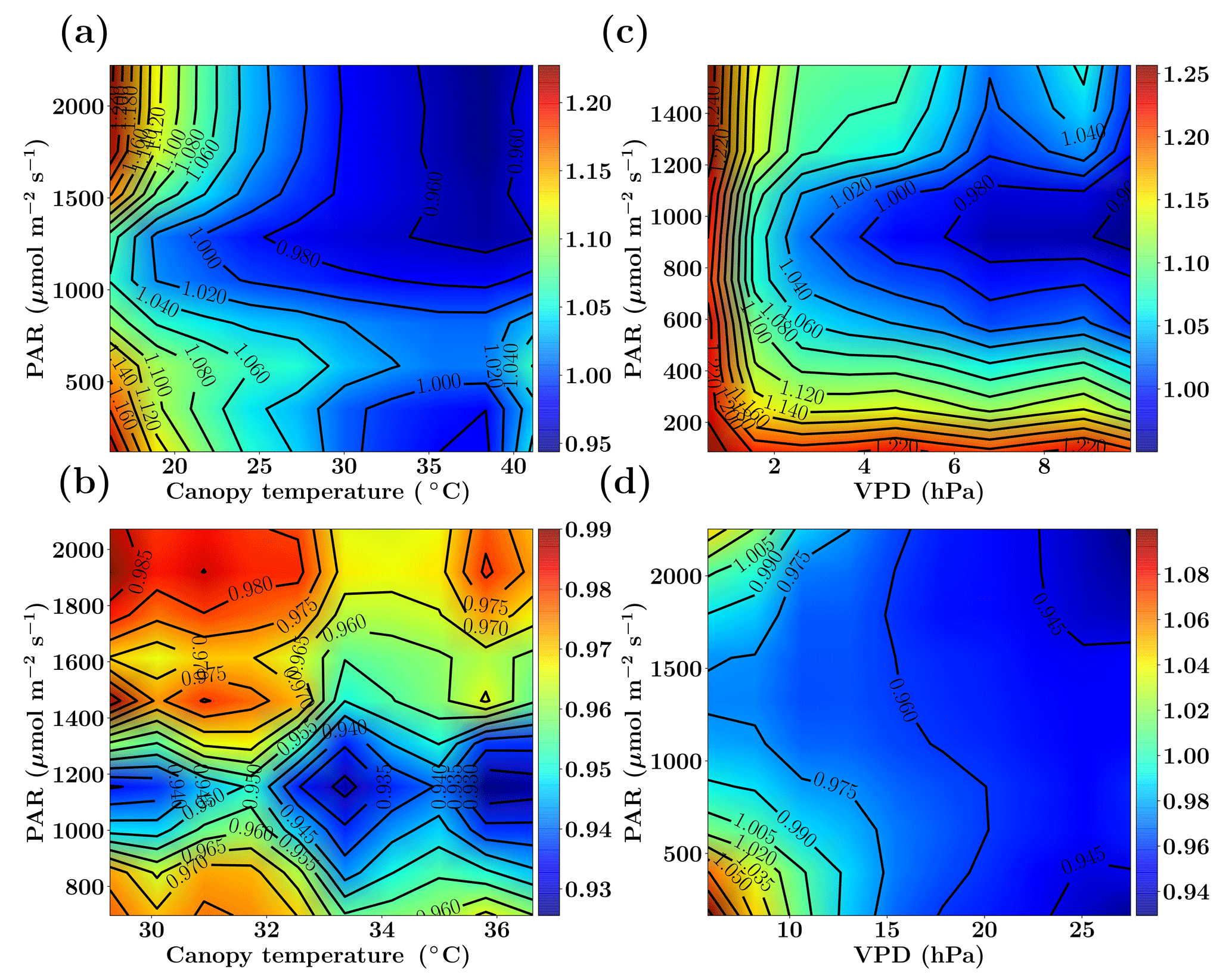
https://www.biogeosciences.net/16/77/2019/bg-16-77-2019-f02

Figure 2Figure showing the ratio of old and new SCOPE GPP ( $f_{GPP} = \frac{{GPP}_{new}}{{GPP}_{old}}$ ) simulations as a function of PAR, canopy temperature and VPD for the C₃ species. The Missouri Ozark fluxnet site comprising of deciduous broadleaf forests for the year 2009 is used and the SCOPE simulations are driven with identical forcings and parameters for both the new and old simulations, the only difference being the implementation of photosynthesis and its temperature dependence (see text). The left column shows f_GPP as a function of PAR and canopy temperature with data points in the low VPD range of 10–15 hPa (a) and high VPD range of 25–30 hPa (b). The right column shows f_GPP as a function of PAR and VPD with data points in the low temperature range of 10–15 ^∘C (c) and moderate temperature range of 25–30 ^∘C (d).

Download

A number of analyses were performed to study the differences in net response of canopy-level carbon and energy fluxes for both C₃ and C₄ species from the SCOPE model due to modification in photosynthesis implementation (old and new) and its temperature dependence (see Supplement Sect. S1).

Figure 2 shows the comparison between the old and new SCOPE versions as the ratio of overall canopy GPP, which is defined as $f_{GPP} = \frac{{GPP}_{new}}{{GPP}_{old}}$ . This ratio is further represented as a function of the three most important forcing variables: PAR (photosynthetically active radiation), canopy temperature and VPD (vapor pressure deficit). The results for the Missouri Ozark site (see Sect. 6.4.1 for site details) with C₃ plant species for the year 2009 are presented in Fig. 2. For this analysis, the SCOPE model simulations are computed for the entire growing season and the f_GPP values are binned according to the PAR temperature (for specific VPD ranges) and PAR VPD (for specific temperature ranges) as 2-D histograms, of which only the mean ( $f_{{GPP}_{mean}}$ ) is represented in Fig. 2.

We find that over the larger parts of the domain of random variables, f_GPP is around 1 and the maximum change in overall GPP is around 25 %. From Fig. 2, it can be observed that in the case of C₃ species, for the combinations of higher canopy temperature and low VPD values (panel a), the new GPP values remain the same or are reduced by about 5 %, although from Fig. 1 we find an increase in the V_cmax response at >25 ^∘C temperature, which may indicate photosynthesis being limited by light instead of the enzyme rubisco. For the combination of low canopy temperature and lower VPD values (panel c), f_GPP values are close to 1 (except for very low PAR/VPD values and with a maximum of about 4 %–6 % increase), which can be explained by an almost identical V_cmax response at lower temperatures in Fig. 1. At high PAR values with higher temperatures (25–30 ^∘C) and low VPD values (panel d) we find that GPP increases by about 6 %–14 %, which can be directly explained by the new increased V_cmax response in that temperature range as indicated in Fig. 1. The results for a similar comparative study with C₄ species is presented in the Sect. S1. Overall, we find that the new model implementation of photosynthesis and its temperature dependence as well as A−C_i iterations works well and only result in moderate, yet noticeable changes. It also underlines that tabulated model parameters can only be optimized for a specific model implementation, which is not necessarily universally transferable to other carbon cycle models.

3 Formulation of inverse problem

The problem of ecosystem flux computation (e.g. GPP, latent energy) from meteorological variables (e.g. VPD, air temperature, relative humidity) and other ecosystem parameters can be represented as follows:

\begin{matrix} (1) & Y = F (X^{'}) + ε, \end{matrix}

where $F () : X^{'} ⟶ Y$ is a functional representation of the model, which maps the model input and parameter space (X^′) quantitatively to the space of ecosystem fluxes (Y), and ε represents the residual error which includes the precision error, the model error and random errors. In our case, SCOPE represents the forward model ℱ(), which is complex and moderately nonlinear, representing a range of physics and canopy physiological processes. We can further represent our forward problem as follows:

\begin{matrix} (2) & Y = F (X; p) + ε, \end{matrix}

where X represents the state vector of parameters to be retrieved, p ( $X, p \subset X^{'}$ and $X^{'} = X \cup p$ ) is a vector of parameters which represents those quantities that influence the measurement and are known with some accuracy but are not meant to be retrieved. We call these parameters the forward functional parameters. In our example p represents the set of all fixed model (SCOPE) parameters not involved in the retrieval. The error term ε represents the measurement noise (e.g. noise or errors in the flux measurements). Given a set of measurements Y, the optimal state vector $\hat{X}$ can be obtained by a generalized inverse method ℛ represented as follows:

\begin{matrix} (3) & \hat{X} = R (Y, \hat{p}, X_{a}, c), \end{matrix}

where $\hat{p}$ represents the best estimate of the forward function parameters. The parameters X_a and c represent the parameters that do not appear in the forward function but they do affect the retrieval and are associated with uncertainties. X_a represents the prior estimate of X and c represents any other parameters in the retrieval scheme as a catch-all for anything else that is used in the retrieval method, which also includes the convergence criteria.

4 Linearization of the forward model

A basic prerequisite for inverting the forward model is to compute its sensitivity with respect to input parameters, i.e. the partial derivatives with respect to all the state vector elements (Jacobi matrix). For linear models, the Jacobians are independent of the actual state. In our case, the SCOPE forward model is moderately nonlinear and its Jacobians need to be computed numerically as analytical methods are currently lacking and hard to implement given some peculiarities in the FvCB equations.

With the Jacobian matrix and a simple forward model call, we can thus write a first-order Taylor expansion for the forward model

\begin{matrix} (4) & F (X; p) = F (X; p)_{X = X_{l}} + {\frac{δ F}{δ X}|}_{X = X_{l}} (X - X_{l}), \end{matrix}

where X_l is an arbitrary linearization point, and $\frac{δ F}{δ X}$ is the partial derivative or Jacobian at the point X=X_l.

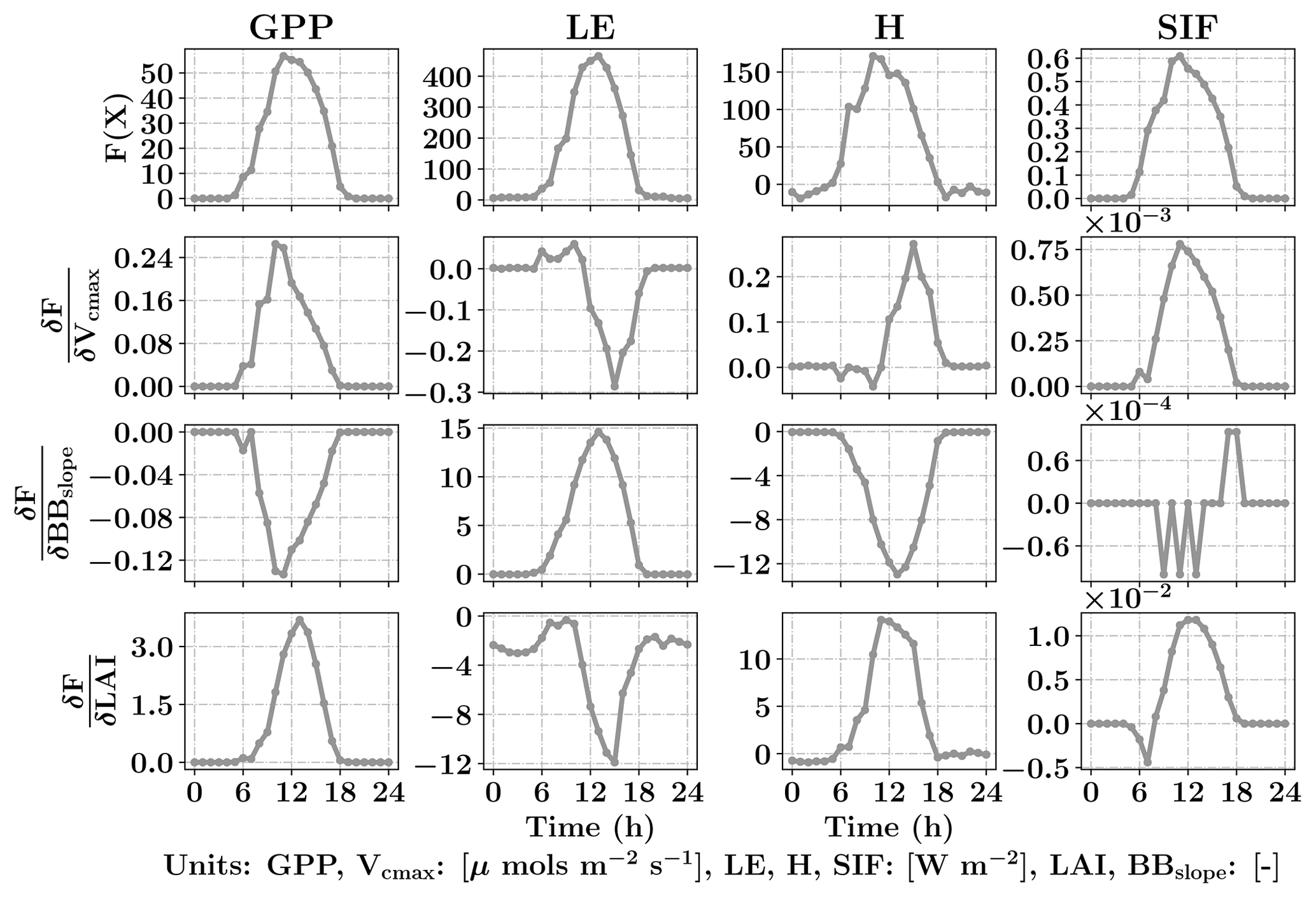
https://www.biogeosciences.net/16/77/2019/bg-16-77-2019-f03

Figure 3Diurnal variability of GPP, LE, H and SIF from SCOPE model simulations (top row) for a typical day in the growing season (3 August 2010) for C₄ corn using data from the Nebraska Mead-1 flux tower site with parameter values V_cmax=50 µmols m⁻² s⁻¹, BB_slope=7 and LAI =4. Second, third and fourth rows from the top shows the diurnal variability in the gradient of GPP, LE, H and SIF with respect to the parameters using SCOPE with positive perturbations δV_cmax=5 µmols m⁻² s⁻¹, δBB_slope=1 and δLAI =0.5 which constitutes the Jacobian matrix for the inversions. It can be observed that the Jacobian matrix is nonlinear with maximum values near the midday period. Our retrieval framework uses concatenated 3-day GPP and LE fluxes (modeled and observed) and their gradients successively within a 3-day window.

Download

5 Iterative retrieval algorithm setup

In the remainder of the paper, we will omit the vector of forward model parameters p which are not a part of the retrieval framework. For the nonlinear problem we use the maximum a posteriori approach. The Bayesian solution for the nonlinear inverse problem where the forward model is a general function of the state, the measurement error is Gaussian (S_ε) and with a prior estimate of the state (X_a) with a Gaussian uncertainty in the prior state (S_a) (Rodgers, 2000) can be represented as follows:

\begin{array}{l} - 2 \ln P (X | Y) & = [Y - F (X)]^{T} S_{ε}^{- 1} [Y - F (X)] \\ (5) & + [X - X_{a}]^{T} S_{a}^{- 1} [X - X_{a}] + c^{'}, \end{array}

where c^′ is a constant. Our aim is to find the best estimate of the state vector $\hat{X}$ (denoted as X henceforth) and an error characterization that describes the posterior PDF. The Gauss–Newton iteration steps for determining the state vector is given by the following:

\begin{array}{l} X_{i + 1} & = X_{i} + (S_{a}^{- 1} + K_{i}^{T} S_{ε}^{- 1} K_{i})^{- 1} [K_{i}^{T} S_{ε}^{- 1} [Y - F (X_{i})] \\ (6) & - S_{a}^{- 1} [X_{i} - X_{a}]], \end{array}

where K_i is the Jacobi matrix. A brief derivation of Eq. (6) is presented in Appendix C; for a more in-depth treatment the reader is referred to Rodgers (2000).

5.1 Levenberg–Marquardt method

In general, the Gauss–Newton iterations discussed previously finds the minimum in one step if the cost function is quadratic with respect to X. However, in our case the cost function is not perfectly quadratic and the initial guess potentially far away from the solution, thus requiring multiple iterations. In addition, the nonlinearity of the problem sometimes results in steps that would actually increase rather than decrease the fit quality. In order to overcome this issue Levenberg (1944) and Marquardt (1963) proposed the following iteration for nonlinear least-squares problem:

\begin{matrix} (7) & X_{i + 1} = X_{i} + ({KK}^{T} + γ_{i} D)^{- 1} K^{T} [Y - F (X_{i})], \end{matrix}

where γ_i is chosen at each step to minimize the cost function and D is a diagonal scaling matrix to scale the elements of the state vector. It can be noted that for γ_i→0, Eq. (7) leads to a Gauss–Newton iteration step and for γ_i→∞ Eq. (7) tends to steepest descent and further the step size tends to 0. It is also expected that the cost function will decrease corresponding to the decrease in γ_i from infinity to zero. The value of γ_i is sequentially updated at each iteration by evaluating the change in cost function. Here, we follow the general recommendations as outlined in Marquardt (1963) and Rodgers (2000).

The guidance for choosing the scaling matrix D is that it must be positive definite. For the current problem we choose it to be $S_{a}^{- 1}$ (as in Rodgers, 2000) and apply the Levenberg–Marquardt (LM) modification to the Gauss–Newton method (iteration Eq. C8), resulting in the following iterative inversion scheme:

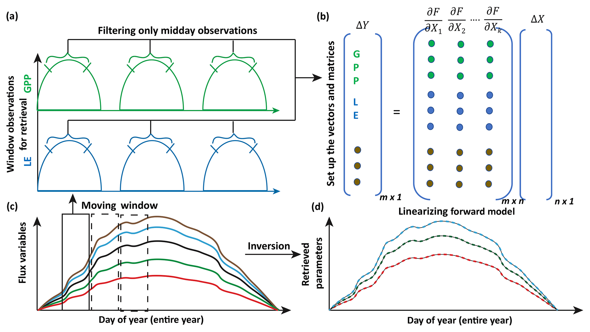
\begin{array}{l} X_{i + 1} & = X_{i} + [(1 + γ) S_{a}^{- 1} + K_{i}^{T} S_{ε}^{- 1} K_{i}]^{- 1} \\ (8) & {K_{i}^{T} S_{ε}^{- 1} [Y - F (X_{i})] - S_{a}^{- 1} [X_{i} - X_{a}]} . \end{array}

https://www.biogeosciences.net/16/77/2019/bg-16-77-2019-f04

Figure 4Illustration of moving window inversion retrieval setup. The bottom left part illustrates the annual ecosystem time series flux variables used for driving the SCOPE model. A 3-day time window is selected for each retrieval in the yearly growing season and a time filter is implemented for concatenating the measurement vector (flux tower observations, with each color representing a different observation variable) of length m in the retrieval windows. The top right shows the vector and matrix setup and the linearization of the forward model. ΔY represents the difference between concatenated observation and modeled vector and ΔX represents the corresponding change in the state vector comprising of n variables (parameters). The bottom right shows the retrieved model parameters after implementing the moving window approach.

Download

5.2 A moving window setup of the inversion problem using flux tower observations

The top row of Fig. 3 shows the SCOPE model simulations of GPP, LE, H and SIF for one day (3 August 2010) in the growing season for C₄ corn using data from the Nebraska Mead-1 flux tower site with parameter values V_cmax=50 µmols m⁻² s⁻¹, BB_slope=7 and LAI =4. The second, third and fourth rows from the top show the numerically computed partial derivatives of GPP, LE, H and SIF with respect to the parameters using SCOPE with positive perturbations δV_cmax=5 µmols m⁻² s⁻¹, δBB_slope=1 and δLAI =0.5. Each column of Fig. 3 represents a row of Jacobian matrices used for the inversions. The figure clearly demonstrates the influence of each of the parameter variables in the state vector (X) on the modeled fluxes (F(X)). We can observe the counteracting nature of variables and the fluxes from the Jacobian. For example, for LE flux, BB_slope has a positive gradient but LAI has a negative gradient. The decrease in LE is attributed to less radiation reaching the soil and a corresponding increase in soil aerodynamic resistance. In this case the canopy resistance goes up but does not compensate for the decreased soil evaporation and results in low sensitivities. Similarly we find V_cmax has a positive gradient for GPP but a negative one for LE, which may again be attributed to the soil evaporation responding to soil temperature. It can be noted that the nature of these sensitivities at the canopy level are sometimes counterintuitive from their leaf-level mechanisms and may vary depending on environmental conditions, such as incoming PAR as well as air temperature and vapor pressure deficit. This also creates diversity in the Jacobians over the diurnal cycle, which allows us to derive more than two parameters from two sets of measurements (GPP and LE). In Fig. 3, we have not only shown derivatives of GPP and LE but also H and SIF (not used here). In this paper, we outline the general framework of parameter inversion, which can easily be modified to make use of more measurements such as H, SIF, reflectance or thermal emissions, all of which can be modeled with SCOPE.

For setting up the observation vector Y_m×1 (see Eq. 8), we use observations of carbon and latent energy fluxes from eddy covariance tower time series records. The observational error matrix (S_ε[m×m]) is assumed to be a diagonal matrix and computed using noise standard deviation as 10 % of the half-hourly to hourly observations (Leuning et al., 2012). We use an initial prior state value of the state vector (X_a[n×1]) as well as the prior error covariance matrix (S_a[n×n]). As mentioned previously, the Jacobian matrix K_m×n is computed numerically by a small perturbation to the value of the state vector X_i+δ (see Fig. 3) at a particular iteration step. The observed (Y) and modeled (F(X)) fluxes in the inversion framework are set up as a long concatenated vector as shown in Fig. 4. The concatenation of different flux variables is done using a time filter to represent the part of the day we wish to include in the retrieval framework as illustrated in Fig. 4. This is logical as we have already demonstrated in Fig. 3 that the gradients are variable throughout the day. Ideally, the time filter applied for concatenating the data should capture the maxima and a range of variations in the gradients, but at the same time reduce the data points to make the retrieval computationally efficient and further tend towards providing stable solutions (retrievals) of the parameter values. Further, the time filter helps to eliminate the nighttime anomalies in the observations for accurate parameter estimation. For other observations such as spectral reflectance a daily noontime average is suitable for concatenation in the observations Y. The assumptions behind the long-term (seasonal) retrieval of important ecosystem and plant physiological parameters is that these parameters change significantly over the growing season but at a slower rate compared to and in response to the environmental and meteorological forcing. Thus, the ecosystem parameters can be assumed to be constant over some finite time window. We implement this assumption to set up our inverse parameter retrieval framework for finite N-day contiguous moving windows over the entire growing season (Fig. 4). We extend the 1-day diurnal setup of Y, F(X) and K as shown in Fig. 3 to multiple days for setting up the N-day windows as illustrated by color coding in Fig. 4. After computing the necessary vectors and matrices for the N-day window, iterations are performed by applying the LM algorithm until convergence to obtain the posterior estimation of the state vector. The retrieval window is moved over to the contiguous next N days and the process is repeated. The retrieval proceeds thus for the entire length of the growing season (Fig. 4). For our retrieval example, we choose a 3-day moving window which seems optimal for the plant response in terms of the photosynthesis parameters (V_cmax, BB_slope and LAI) towards the change in environmental drivers.

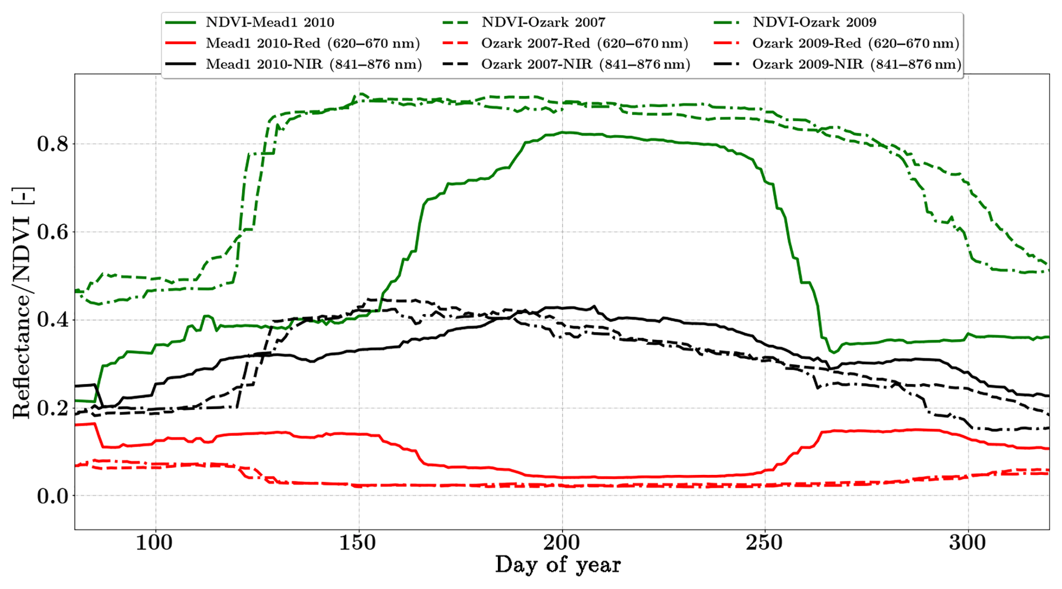
https://www.biogeosciences.net/16/77/2019/bg-16-77-2019-f05

Figure 5Figure showing the seasonal variability of red, NIR MODIS nadir reflectance and NDVI for the Nebraska Mead-1 and Missouri Ozark Site. This dataset is used in SCOPE model inversions in conjunction with fluxes of carbon and water for retrieval of ecosystem parameters.

Download

5.3 Error characterization and convergence criteria for the retrievals

As mentioned in Sect. 5.1, we have selected a convergence criteria for the parameter retrievals in each of the moving windows based on the ratio of the true error to the expected error for each of the iteration steps. The total error minimized for the retrieval is given by $[Y - F (X_{i})]^{T} S_{ε}^{- 1} [Y - F (X_{i})] + [X - X_{a}]^{T} S_{a}^{- 1} [X - X_{a}]$ . However, for testing the convergence within each iteration step, we use the method suggested by Rodgers (2000), which adapts the Levenberg–Marquardt parameter depending on the nonlinearity of the forward model.

After convergence, the posterior error covariance matrix for the retrieved state vector $\hat{X}$ can be computed as follows:

\begin{matrix} (9) & S = [S_{a}^{- 1} + K_{i}^{T} S_{ε}^{- 1} K_{i}]^{- 1} . \end{matrix}

The reduction in error is defined as follows:

\begin{matrix} (10) & ζ_{i} = 1 - {(\frac{S_{j j}}{S_{a_{j j}}})}^{0.5}, \end{matrix}

where S_jj and $S_{a_{j j}}$ represent the diagonal elements in the posterior and prior error covariance matrices respectively. In our LM retrieval process, we use the retrieved state vector $\hat{X}$ of the previous window as the first guess (but not prior) for the current window. This saves computational cost and is based on the assumption that our state vector varies smoothly in time.

6 Results for implementing the inversion framework in SCOPE

In this section, we discuss the results of optimal parameter estimation by applying the Bayesian inversion framework to three different ecosystems. The aim is to demonstrate the applicability for the retrieval (as well as capturing the seasonal variability) of canopy structural and photosynthesis parameters using carbon and water fluxes, and to further compare and contrast the results across the different ecosystems. In order to demonstrate the greater potential of SCOPE in modeling spectrally resolved reflectance (not found in other general carbon cycle models) and versatility of the inversion framework we have also incorporated Moderate Resolution Imaging Spectrometer (MODIS) satellite reflectance bands in the retrievals. We further demonstrate how reflectance and fluxes are able to better constrain parameters such as V_cmax, BB_slope and LAI compared to just using flux tower observations.

6.1 Data filtering criteria in the moving window retrievals

Apart from the overall algorithmic steps as described previously, we apply the following filter criteria on the results and the data for a computationally efficient retrieval.

In constructing the observation vector Y we apply a time-of-the-day filter (e.g. data between 09:00 and 16:00 LT and so on) for the initial forward SCOPE model.
For computing the Jacobians, a PAR-based threshold (PAR >100 µmols m⁻² s⁻¹) is applied to ensure sensitivity of the measurement vector with respect to state vector variations and to minimize the occurrence of unreasonable flux tower data (high fractional errors).
A filter is implemented to check and ensure that the state vector remains positive at every iteration. If somehow due to a small enough γ the state vector is negative, the γ value is adjusted in an iterative manner to keep it within bounds.

6.2 MODIS satellite reflectance data

We use the daily MODIS MCD43A reflectance product in this study (Schaaf and Wang, 2015). The spatial resolution of the dataset is 500 m and bands 1 and 2 (red and NIR) centered at 620 and 841 nm respectively were used in the inversion. These data are adjusted using a bidirectional reflectance distribution function to model the values as if they were collected from a nadir view. Figure 5 shows the distinct seasonality in greenness which is represented by NDVI over the two sites. SCOPE models the full Nadir VSWIR spectral reflectance (400 to 2500 nm) from which values corresponding to the two MODIS reflectance bands are extracted and used concurrently with the observations in the inversion framework.

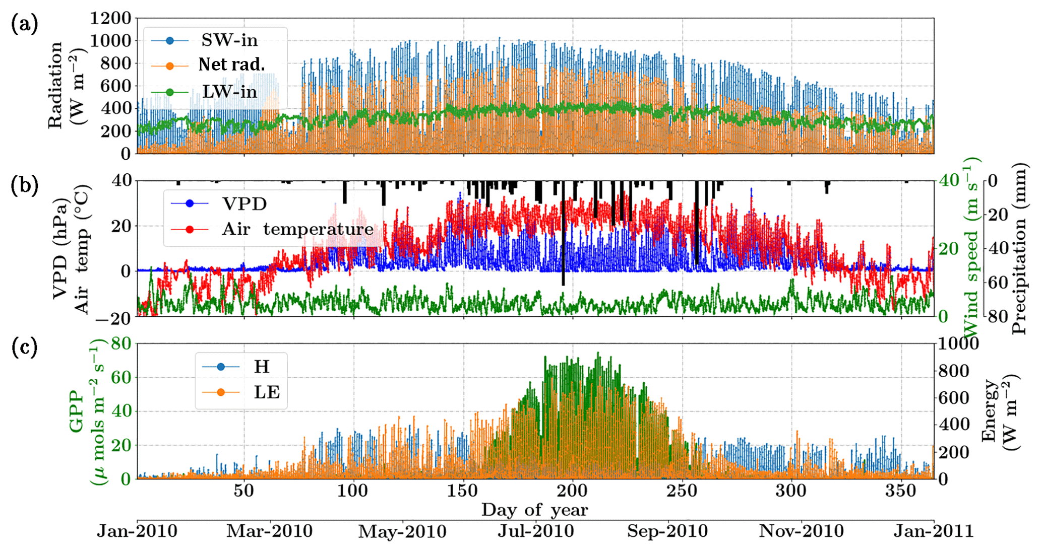
https://www.biogeosciences.net/16/77/2019/bg-16-77-2019-f06

Figure 6Figure showing the diurnal and seasonal variability of important environmental and meteorological forcings together with the tower observed fluxes of carbon and energy used in SCOPE model inversions for the Nebraska Mead flux tower site. The variables in (a) and (b) are used as inputs to the SCOPE model and the variables in (c) are used as a target in a moving window retrieval approach.

Download

6.3 Retrieval results for the Nebraska Mead-1 site

6.3.1 Site description

The Nebraska Mead-1 site is a part of the AmeriFlux network, located in Lincoln, Nebraska, and is one of the three cropland sites at the University of Nebraska Agricultural Research and Development Center, with continuous data records from 2001 until the present (Suyker et al., 2005). This site is a continuously irrigated corn (C₄, species) crop site, with mean annual precipitation of 790 mm and mean annual temperature of 10.07 ^∘C. We choose the year 2010 and an hourly time resolution for the analysis. The site meteorology and forcing variables relevant to the SCOPE inversion retrievals are shown in Fig. 6. The top two panels show the environmental forcing variables which are used as input (except precipitation) in the SCOPE simulations. The bottom panel represents carbon (GPP) and energy (LE, H) fluxes, which are used to construct the observation vector Y. The figure indicates that the growing season extends from around June through September, coinciding with high temperature, VPD and net radiation. We focus on the retrieval of the parameters V_cmax, BB_slope and LAI during this entire growing season.

Table 1Prior values for LM inversion (units: V_cmax, µmols m⁻² s⁻¹; BB_slope, no unit; LAI, no unit).

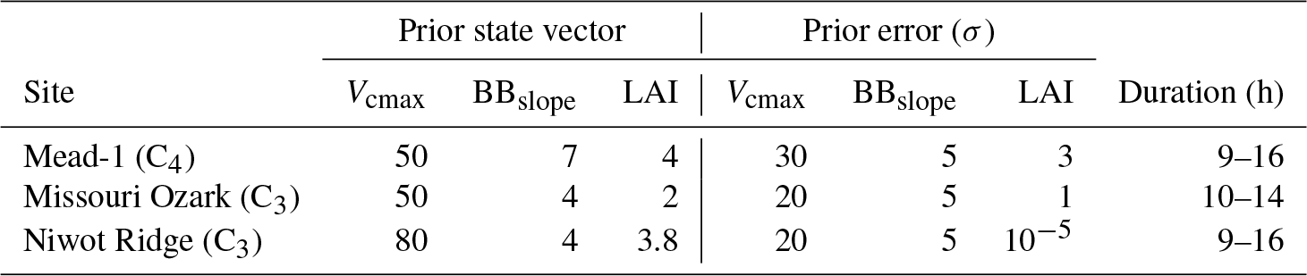
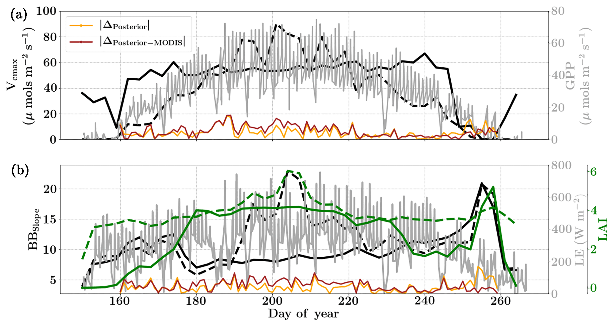
Download Print Version | Download XLSX

https://www.biogeosciences.net/16/77/2019/bg-16-77-2019-f07

Figure 7Figure showing the seasonal variability in retrieved parameter values of V_cmax, BB_slope and LAI for the Nebraska Mead-1 site using a 3-day moving window inversion approach for the year 2010. The actual points in the time series (grey lines) of the GPP and LE fluxes used as the target observations (Y) for the moving window inversion approach are shown in the background. The figure shows the comparison of the retrieved parameters using only GPP and LE fluxes (shown as dashed lines) as well as using a combination of fluxes and MODIS reflectance (shown as solid lines). The results show reasonable trends in the retrieved parameters along with their sensitivity to GPP and LE fluxes across the growing season.

Download

6.3.2 Inversion parameters and results

For each of the retrieval windows, the prior value of the state vector along with prior errors and daytime duration, which is used for filtering the GPP and LE observations, are shown in Table 1. Here, we use a purely diagonal prior error covariance matrix, with zero off-diagonal elements. Figure 7 shows the retrievals of parameters V_cmax, BB_slope and LAI. The grey time series of GPP and LE values in the background are the actual filtered values used for constructing the observation (Y) vector corresponding to each retrieval window. The dashed lines indicate the retrieved parameters using only GPP and LE fluxes. The solid lines indicate the retrieved parameters using the fluxes together with MODIS reflectance. The orange (with fluxes only) and brown (with fluxes and MODIS red and NIR reflectance) lines show the result of posterior simulations of fluxes with the optimized parameters. These lines represent the absolute daily average posterior simulation errors ( $Δ = | Observed - Posterior |$ ) in the fluxes without and with the use of MODIS reflectance along with the flux observations in the inversions.

We find a seasonal variability in the retrieved parameters, which follow a similar pattern in GPP or LE. In particular, the retrieved LAI as well as V_cmax shows a similar seasonality to GPP. There is also some variability in retrieved BB_slope, which is correlated with LE observations. We found that including MODIS reflectance places better constraints on the parameters during the peak of the growing season, with much less variability in retrieved LAI and V_cmax.

As expected, the optimized parameters using just flux observations (dashed lines) are quite sensitive to the variation in GPP and LE, for example around DOY 190 and 210, where there is sudden dip in the retrieved V_cmax. Including the MODIS reflectance (solid lines) in the inversions alleviates most of these large variabilities due to fluctuations in the observed fluxes or meteorology. Moreover, with this additional MODIS reflectance constraint the range of variability for all the three parameters V_cmax, BB_slope and LAI is more realistic. The comparison of posterior simulations (brown and orange lines) indicates the net errors in the prediction of fluxes are quite similar in both cases (with and without MODIS reflectance) with the difference between the two being δ_Δ≤15 % during the middle of the growing season. This may indicate that in this example there is an equifinality in the posterior simulation of fluxes with the retrieved parameters, which gets alleviated with the reflectance data. We find that the MODIS reflectance better constrains LAI during the beginning of the growing season between DOY 160 and 180. The unexpectedly large increases in BB_slope and LAI around DOY 250–260 may be partially attributed to the largest rainfall events (see Fig. 6). Part of this variability and correlation between BB_slope and LAI may also be due to the diminishing role of soil evaporation (parameterized by a single resistance in SCOPE) with increasing LAI. Another part may be due to evaporation from the wet canopies, which is not currently represented in SCOPE. This may cause the inversion to overestimate BB_slope, even though it would not represent the gas exchange through the stomata. From the inversion results it is clear that all three parameters V_cmax, BB_slope and LAI are much better constrained (with more realistic values and better seasonal variability) with the assimilation of reflectance data together with fluxes in the optimal estimation framework.

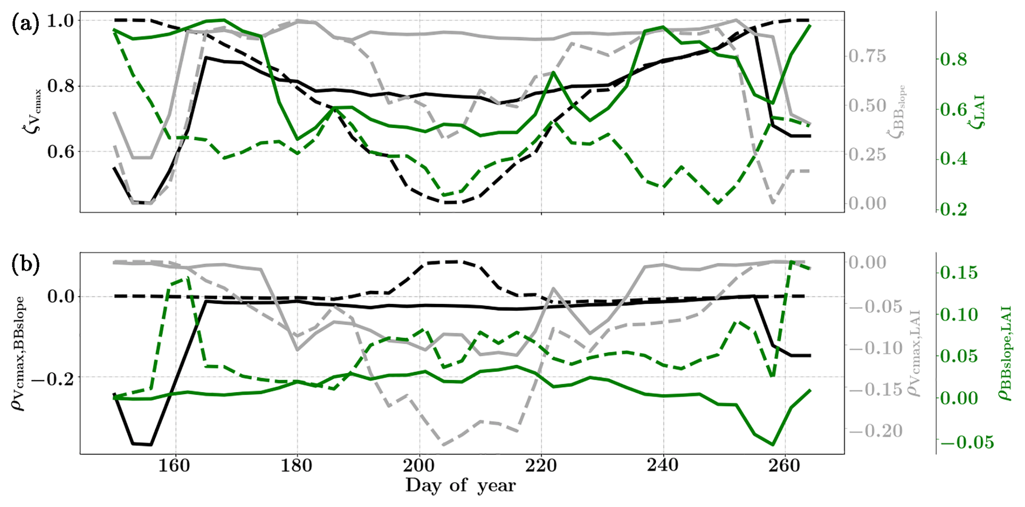
https://www.biogeosciences.net/16/77/2019/bg-16-77-2019-f08

Figure 8Figure showing the seasonal variability of the posterior error reduction (ζ) and correlation coefficient of the retrieved parameter values of V_cmax, BB_slope and LAI for the Nebraska Mead-1 site using a 3-day moving window inversion approach for the year 2010. Panel (a) shows the $ζ_{V_{cmax}}$ , $ζ_{{BB}_{slope}}$ and ζ_LAI for the entire growing season and (b) shows the correlation coefficients (normalized off-diagonal elements of posterior error covariance matrix) among these variables. The results of retrievals using only GPP and LE fluxes are shown as dashed lines and the results using a combination of fluxes and MODIS reflectance are shown as solid lines. Both the ζ and correlation coefficients are computed using the final Jacobian matrix at the end of each retrieval window.

Download

Figure 8a shows the final posterior error reduction (ζ_i-Eq. 10) of the retrieval iterations for each moving window. The dashed lines indicate retrieval results using GPP and LE observations only and the solid lines show retrievals that use reflectance observations in addition. The value of ζ_i is computed from the diagonal elements of the posterior error covariance matrix. We find a significant reduction in the posterior errors of the variables in the state vector. There is a strong seasonality in $ζ_{V_{cmax}}$ and ζ_LAI values and moderate to no seasonality for the $ζ_{{BB}_{slope}}$ . It can be clearly seen that the posterior error reduction is significantly greater (∼50 %) when combining the reflectance data with the flux observations. The error reduction provides more confidence in the retrieved parameters, which are also more realistic. The posterior error covariance matrix also indicates whether the retrieved parameters are truly independent (as in the case of a diagonal matrix) or whether they covary (indicated by significant off-diagonal elements). The error correlation is given by $ρ_{x, y} = \frac{COV (x, y)}{σ_{x} σ_{y}}$ and should be considered when interpreting covariations of retrieved parameters as the nature and magnitude of the associations between the variable pairs are true for the retrievals only and may or may not represent the behavior of the variable pairs in nature due to different environmental conditions. Figure 8b shows the growing season error correlation patterns between the three parameters from the retrievals. From the results which include reflectance data with flux observations, it can be seen that during the peak growing season $ρ_{{BB}_{slope, LAI}}$ and $ρ_{V_{cmax, LAI}}$ have opposite signs, indicating slightly positive and negative association between the variable pairs in the retrievals. These trends are also true when only flux data are used for the retrievals. However, in comparison $ρ_{V_{cmax}, {BB}_{slope}}$ is mostly zero but has opposite signs with and without reflectance data and thus indicates both favorable and competing effects during the middle of the growing season.

Finally, Fig. 9 demonstrates the net improvement in canopy GPP and LE fluxes due to the optimized state vector using flux observations only over their prior values. The first column represents the diurnal and seasonal variability in the time series of GPP and LE fluxes with optimized and unoptimized parameters and further its comparisons with flux tower values. The right column represents the one-to-one comparisons of the same. We find a significant improvement in the estimation of GPP (R²=0.94) and the optimized parameters are able to capture the growing seasonal variability well as measured by flux tower observations (slope =1.04). The improvement in modeling the fluxes with the posterior over the prior value of the state vector is also captured by the χ² error statistic ( $χ^{2} = \sum_{i = 0}^{k} ((y_{i} - F (x_{i})) / σ_{i})^{2}$ ) for the prior (unoptimized) and posterior (optimized) simulations. 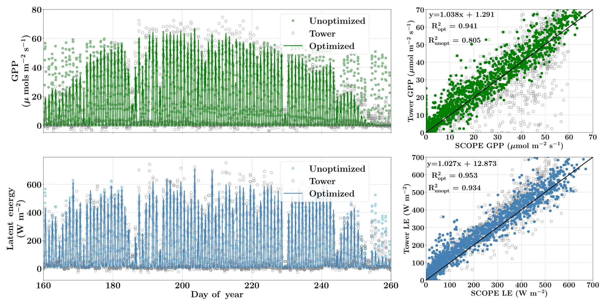The corresponding values are $χ_{GPP - opt}^{2} = 9382$ , $χ_{GPP - unopt}^{2} = 10 728$ , $χ_{LE - opt}^{2} = 19 235$ and $χ_{LE - unopt}^{2} = 20 554$ .

https://www.biogeosciences.net/16/77/2019/bg-16-77-2019-f09

Figure 9Figure showing the improvement in diurnal and seasonal variability in modeling the GPP and LE fluxes with optimized parameters over prior values using SCOPE for the Nebraska Mead-1 site for the year 2010. The figure also shows the one-to-one comparison (indicated by the black line) with the observed flux tower values. The optimization of the photosynthetic parameters improves the accuracy of computing the carbon and water fluxes as indicated by the R² value and the equation of the regression line.

Download

6.4 Retrieval results for the Missouri Ozark site

6.4.1 Site description

The Missouri Ozark site is also a part of the AmeriFlux network and is located in the University of Missouri Baskett Wildlife Research area, situated in the Ozark region of central Missouri. It is uniquely located in the ecologically important transitional zone between the central hardwood region and the central grassland region of the US (Gu et al., 2006). This site has a mean annual precipitation of 986 mm and a mean annual temperature of 12.11 ^∘C and has continuous data records from 2004 until the present. It is a deciduous broadleaf forest site comprised of C₃ plant species. We use half-hourly datasets from the year 2007 and 2009 in the present analysis. The site meteorology and forcing variables relevant to the SCOPE inversion retrievals are shown in Figs. S4 and S5 in the Supplement. From the meteorological data it can be seen that the year 2009 was a normal wet year and the year 2007 was a year with a midsummer drought around DOY 250. This is also reflected in observed GPP and LE fluxes with two distinct peaks in the growing season, caused by a late-summer drought and associated low productivity around DOY 250. This decrease in productivity is not distinguishable from the MODIS reflectance data in Fig. 5, which indicates that plants maintain greenness during this time, making this a unique test case for our inversion setup as the V_cmax fits reflect the stress factor as well, which is usually applied to downscale the physiological V_cmax during environmental stress. We focus on the retrieval of the parameters V_cmax, BB_slope and LAI during this entire (longer) growing season. For both years we demonstrate the parameter retrievals using GPP and LE fluxes only as well as compare our retrievals using additional constraints of MODIS red and NIR reflectances (Fig. 5).

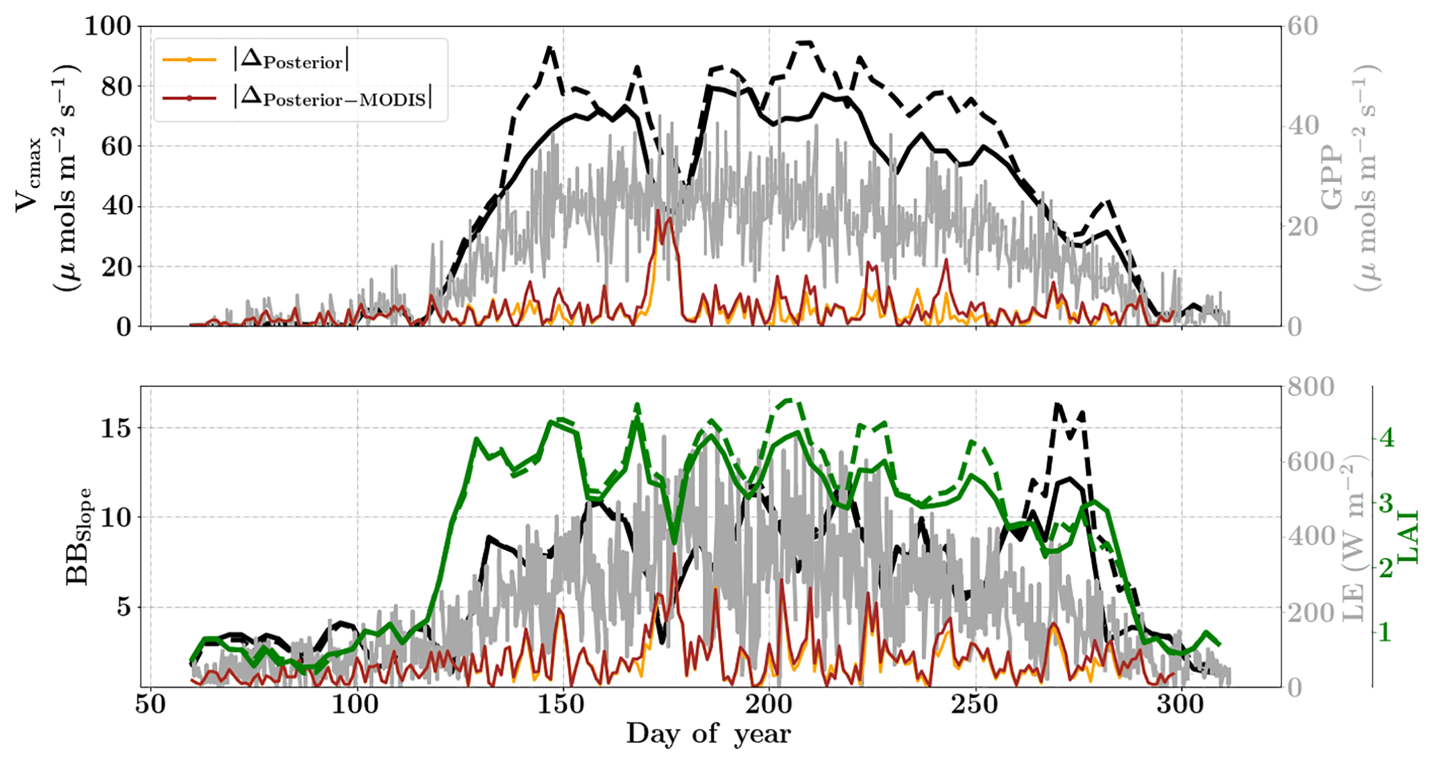
https://www.biogeosciences.net/16/77/2019/bg-16-77-2019-f10

Figure 10Figure showing the seasonal variability in retrieved parameter values of V_cmax, BB_slope and LAI for the Missouri Ozark site using a 3-day moving window inversion approach for the year 2009. The actual points in the time series (grey lines) of the GPP and LE fluxes used as the target observations (Y) for the moving window inversion approach are shown in the background. The figure shows the comparison of the retrieved parameters using only GPP and LE fluxes (shown as dashed lines) as well as using a combination of fluxes and MODIS reflectance (shown as solid lines). The results show reasonable trends in the retrieved parameters along with their sensitivity to GPP and LE fluxes across the growing season.

Download

https://www.biogeosciences.net/16/77/2019/bg-16-77-2019-f11

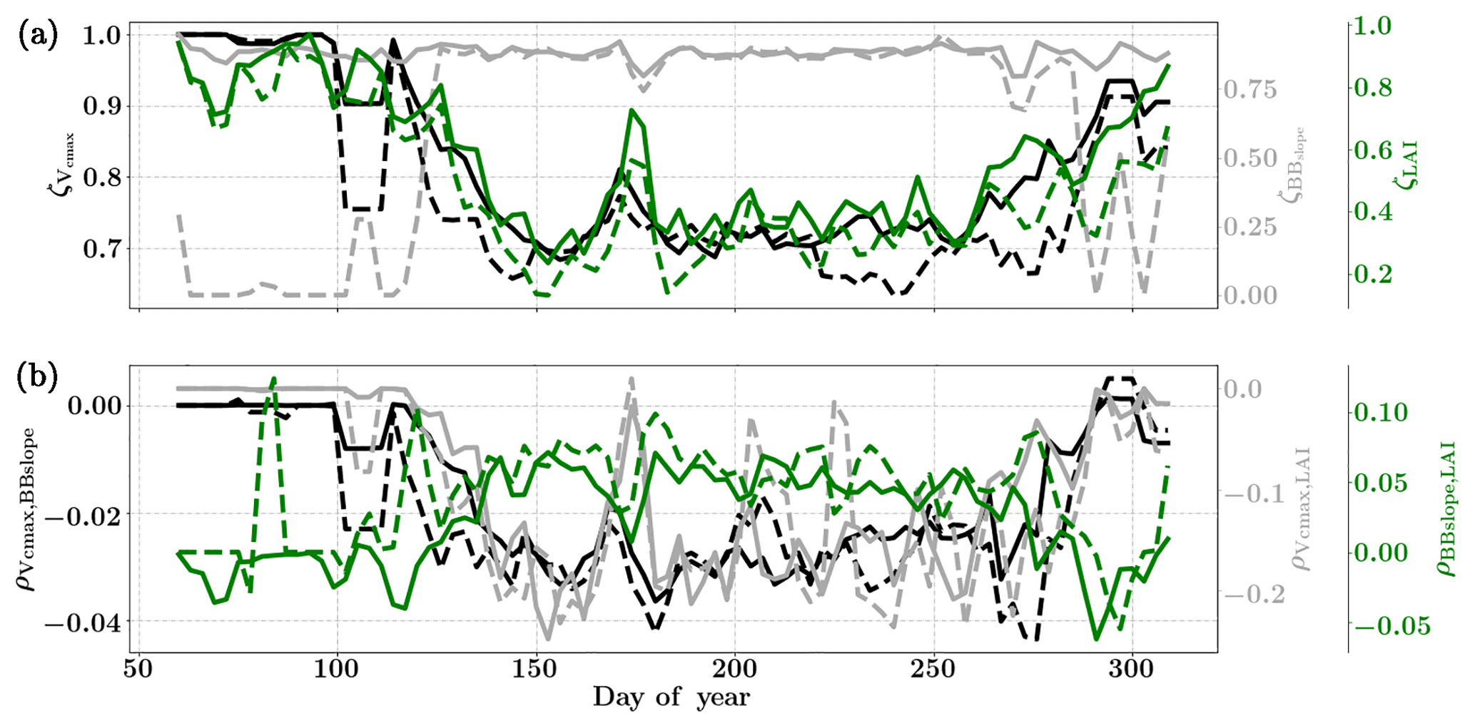
Figure 11Figure showing the seasonal variability of the posterior error reduction (ζ) and correlation coefficient of the retrieved parameter values of V_cmax, BB_slope and LAI for the Missouri Ozark site using a 3-day moving window inversion approach for the year 2009. Panel (a) shows the $ζ_{V_{cmax}}$ , $ζ_{{BB}_{slope}}$ and ζ_LAI for the entire growing season and (b) shows the correlation coefficients (normalized off-diagonal elements of posterior error covariance matrix) among these variables. The results of retrievals using only GPP and LE fluxes are shown as dashed lines and the results using a combination of fluxes and MODIS reflectance are shown as solid lines. Both the ζ and correlation coefficients are computed using the final Jacobian matrix at the end of each retrieval window.

Download

6.4.2 Inversion parameters and results for the year 2009

The assumed prior values of the state vector, prior errors and daytime duration which are used for filtering the GPP and LE observations for the retrieval windows are shown in Table 1. Compared to Mead, the retrieval for this site is carried out over a much longer duration, covering almost the entire year. Figure 10 (like Mead-1, Fig. 7) shows the comparison of parameter retrievals V_cmax, BB_slope and LAI using (i) only flux observations and (ii) flux observations combined with two MODIS reflectance bands. We find an overall strong seasonality with realistic values of V_cmax, BB_slope and LAI, following the patterns in GPP and LE. The beginning (and end) of the growing season shows increasing (decreasing) trends in V_cmax and LAI retrievals, which coincide well with the increase (decrease) in MODIS NDVI observations (Fig. 5). The retrieved LAI variability helps to explain the rapid appearance of new leaves in the spring (March–April) and their disappearance around fall (October–November). The MODIS reflectance data help to better constrain LAI and V_cmax, which is specifically evident around DOYs 140–150 and 200–250. The sharp increase in retrieved V_cmax when using just the flux observations around DOY 148 may be attributed to the sharp peaks in GPP; however, the reflectance observations clearly help to better constrain the state vector. There are some issues with the retrieval for windows around DOY 175 and 275 (BB_slope); this may again correspond to the large precipitation (see Fig. 4) events (e.g. overestimation of BB_slope) around these windows as well as sharp fluctuations in GPP and LE, respectively. This error in prediction of fluxes ( $Δ = | Observed - Posterior |$ ) is also revealed by posterior simulations represented by brown and orange lines. Comparing the posterior simulations with and without the MODIS reflectance constraints with the prior reveals the net error to be of similar magnitude in both cases with δ_Δ≤15 % during the growing season and indicates equifinality in the predicted fluxes with the parameter combinations.

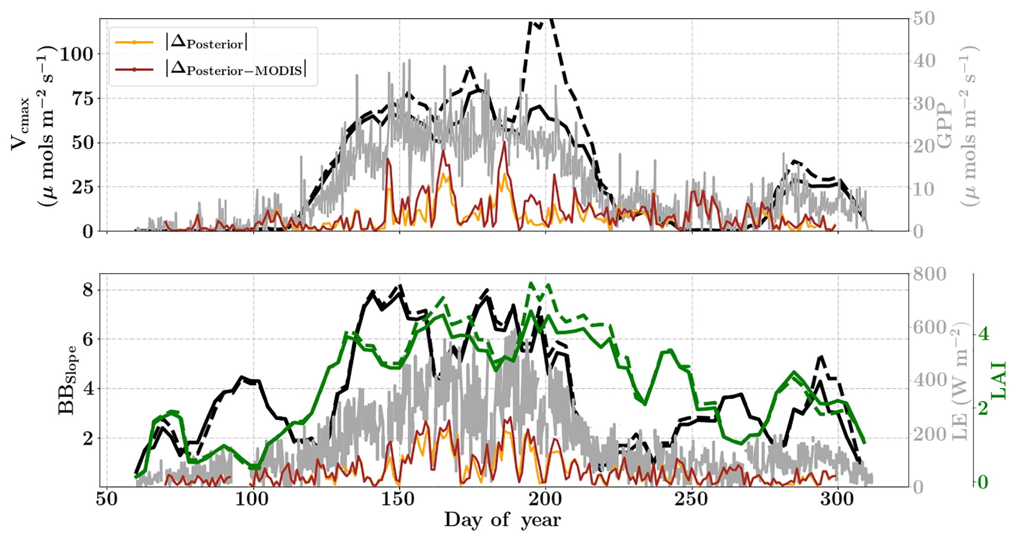
https://www.biogeosciences.net/16/77/2019/bg-16-77-2019-f12

Figure 12Figure showing the seasonal variability in retrieved parameter values of V_cmax, BB_slope and LAI for the Missouri Ozark site using a 3-day moving window inversion approach for the year 2007. The actual points in the time series (grey lines) of the GPP and LE fluxes used as the target observations (Y) for the moving window inversion approach are shown in the background. The figure shows the comparison of the retrieved parameters using only GPP and LE fluxes (shown as dashed lines) as well as using a combination of fluxes and MODIS reflectance (shown as solid lines). The results show reasonable trends in the retrieved parameters along with their sensitivity to GPP and LE fluxes across the growing season.

Download

Figure 11 shows the final posterior error reduction of the retrieval iterations for each moving window. It is found that there is significant reduction in the posterior errors for BB_slope. We find that $ζ_{V_{cmax}}$ and ζ_LAI have the same trend and seasonality as that of retrieved V_cmax and LAI respectively. The evolution of the retrieval error correlations is again interesting and comparison with the Mead Corn-C₄ site using flux observations only shows it is similar for $ρ_{V_{cmax, LAI}}$ and $ρ_{{BB}_{slope, LAI}}$ (negative and positive respectively) and different for $ρ_{V_{cmax}, {BB}_{slope}}$ .

The correlations $ρ_{V_{cmax}, {BB}_{slope}}$ and $ρ_{V_{cmax, LAI}}$ are both negative, indicating counteracting effects of these variables in the retrieval. In comparison, $ρ_{{BB}_{slope, LAI}}$ is positive for the retrievals, indicating in-sync behavior. The error correlations $ρ_{V_{cmax, LAI}}$ are highest among the three in the middle of the growing season.

Finally, there is a significant improvement in the estimation of both GPP and LE fluxes (see Fig. S6) (R²=0.7) with the optimized state vector over the prior values. The optimized state vector is able to capture the growing seasonal variability well (slope of regression lines: GPP =0.97 and LE =1.02). The unoptimized prior values severely underpredict both fluxes. The corresponding error measures $χ_{GPP - opt}^{2} = 12 975$ , $χ_{GPP - unopt}^{2} = 30 070$ , $χ_{LE - opt}^{2} = 17 260$ and $χ_{LE - unopt}^{2} = 32 283$ indicate that the inversion framework is able to retrieve the seasonal dynamics in the photosynthetic and canopy structural parameters for accurate prediction of the fluxes.

6.4.3 Inversion results for the year 2007

The year 2007 for the Missouri Ozark site is an interesting example because the forest experiences a late summer drought and decrease in productivity, which is captured by the flux observations but not with phenology or greenness (see Fig. S5, Figs. 12 and 5). The inversion setup, meteorological data resolution, initial guess and prior errors for the year 2007 are similar to that of 2009. Figure 12 shows the results for the retrieval of parameters V_cmax, BB_slope and LAI from the inversion framework using (i) observations of GPP and LE fluxes (dashed line) and (ii) flux observations with MODIS reflectance bands (solid lines). The overall seasonality of the retrieved parameters reveals that the inversion framework is able to capture the late-summer drought. The midseason drought around DOY 230–250 is well captured by decreases in photosynthesis (V_cmax) and stomatal conductance (BB_slope). These parameters again increase from around DOY 260 after the drought recovery and also correlate well with the flux observations. However, the V_cmax variations should not be confused with actual changes in rubisco concentrations. Like many other carbon cycle models, the only way to impose environmental stress (apart from VPD and temperature) in SCOPE is to scale V_cmax with a stress factor between 0 and 1. Our retrieved effective V_cmax is the product of a stress factor and the physiological V_cmax, which explains the large variations during drought here.

In contrast, the change in retrieved LAI during the period from DOY 240 to 300 is fairly gradual and reflects the phenology only. The addition of MODIS reflectance data constrains LAI (and in conjunction V_cmax) much better than just the flux observations, which is clearly evident from the V_cmax retrievals around DOY 200. This large change in V_cmax (when using just constraining flux observations) also corresponds to the single largest rainfall event of the season (see Fig. S5) as well as a corresponding concurrent spike in productivity. The MODIS red and NIR reflectances, unlike GPP and LE fluxes, were insensitive to this short drought and provide better constraints on the LAI and V_cmax retrievals during this period. A comparison of modeled red and NIR reflectance from the SCOPE model with optimized parameters shows that it matches well with the observations (see Fig. S8). There is excellent match in the red reflectance throughout the season, and the NIR reflectance also matches well with the observations during the early–middle part of the growing season (DOYs 130–250); during the post-drought recovery phase the increase may be attributed to the increase in retrieved LAI. Apart from the drought period, the range and variability of all three parameters correspond well with the retrievals for the same site for the year 2009 presented earlier.

The posterior simulations excluding and including the MODIS observations (represented as orange and brown lines respectively in Fig. 12) indicate similar improvement in prediction of fluxes over their priors with $R_{GPP - opt}^{2} = 0.7$ , $R_{GPP - unopt}^{2} = 0.2$ , $R_{LE - opt}^{2} = 0.5$ and $R_{LE - unopt}^{2} = 0.1$ . For the year 2007 it is also found that the posterior error reduction $ζ_{V_{cmax}}$ and ζ_LAI is similar or slightly better compared to the year 2009 (see Fig. S7). This again provides more confidence in the retrieved parameters and their temporal dynamics. As expected, the posterior error reduction is slightly better for all three parameters with the reflectance constraints during the middle of the growing season. The error correlations $ρ_{V_{cmax}, {BB}_{slope}}$ and $ρ_{V_{cmax, LAI}}$ for 2007 are both negative and similar in magnitude to that of year 2009. The error correlation structure for the year 2007 is different compared to the wet year 2009, especially during the middle of the growing season, and may be attributed to the change in interaction between the state vector elements due to imposed drought stresses. We note that our moving window inversion setup using different observational streams is able to capture the ecosystem dynamics over the entire growing season as well as capture in-season drought dynamics, which are not possible using traditional one-step seasonal or annual inversion approaches. Inversions like this will also help guide model parameterizations of stress impacts on the dynamic down-regulation of photosynthesis as a response to, for example, changes in the soil matric potential.

Finally, we performed sensitivity analyses of the newer temperature dependence implementation in SCOPE on the inversion retrieval results for the Ozark site (see Sect. S1.1.2). It is found that with the newer temperature dependence implementation and optimized parameters SCOPE is able to capture V_cmax variations due to changes in the average canopy temperatures well. There is a clear difference between the retrieved V_cmax with and without temperature dependence, and the changes correlate with the implemented temperature response functions (see Sect. S1.1.2). The results of the posterior simulation on GPP and LE fluxes also indicate improvement with δχ² error reduction of 3415 and 2104 for GPP and LE respectively.

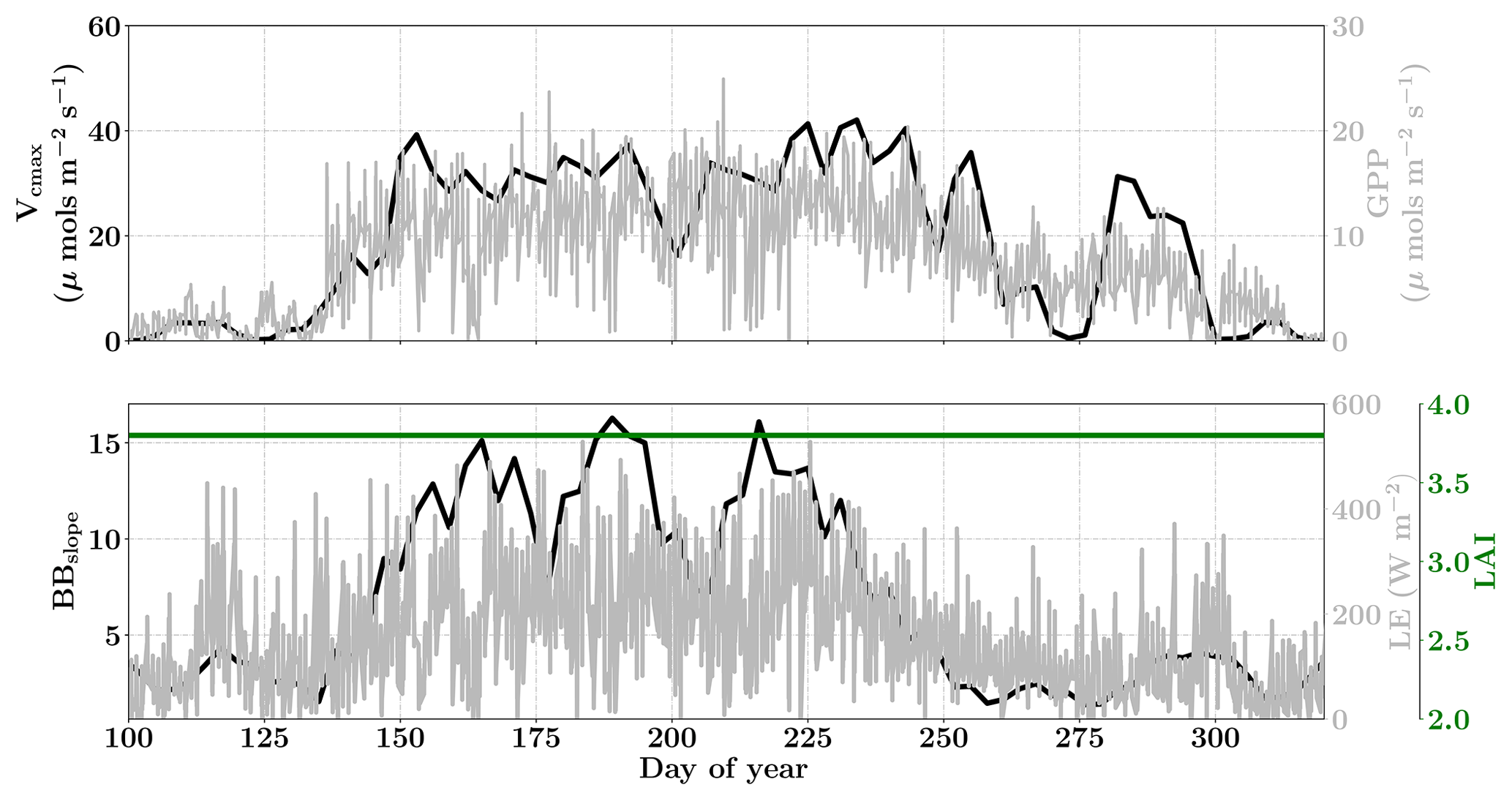
https://www.biogeosciences.net/16/77/2019/bg-16-77-2019-f13

Figure 13Figure showing the seasonal variability in retrieved parameter values of V_cmax, BB_slope and LAI for the Niwot Ridge site using a 3-day moving window inversion approach for the year 2010. The actual points in the time series (grey lines) of the GPP and LE fluxes used as the target observations (Y) for the moving window inversion approach are shown in the background. The results show reasonable trends in the retrieved parameters along with their sensitivity to GPP and LE fluxes across the growing season.

Download

https://www.biogeosciences.net/16/77/2019/bg-16-77-2019-f14

Figure 14Figure showing the seasonal variability of the posterior error reduction (ζ) and correlation coefficient of the retrieved parameter values of V_cmax, BB_slope and LAI for the Niwot Ridge site using a 3-day moving window inversion approach for the year 2010. Panel (a) shows the $ζ_{V_{cmax}}$ , $ζ_{{BB}_{slope}}$ and ζ_LAI for the entire growing season and (b) shows the correlation coefficients (normalized off-diagonal elements of posterior error covariance matrix) among these variables. Both the ζ and correlation coefficients are computed using the final Jacobian matrix at the end of each retrieval window.

Download

6.5 Retrieval results for the Niwot Ridge site

6.5.1 Site description

The Niwot Ridge site is also a part of the AmeriFlux network located in a subalpine forest ecosystem just below the continental divide near Nederland, Colorado. The average elevation of this site is 3050 m and it is one of the high alpine evergreen needleleaf forests with C₃ plant species (Burns et al., 2016). This ecosystem is nearly 100 years old, and thus very different from the Mead and the Ozark sites (Monson et al., 2002). This site has a mean annual precipitation of 800 mm and a mean annual temperature of 1.5 ^∘C and has a continuous data record from 1998 until the present. This site is thus the coldest and driest among the three. We choose the year 2010 for the current analysis, using half-hourly flux data. The site meteorology and forcing variables relevant to the SCOPE inversion retrievals for the year 2010 are presented in the Fig. S11. The snow cover at this site affects the energy exchanges and GPP for a large fraction of the year. The trees are evergreen and there is no well defined growing season but we find that most photosynthetic activity occurs in the period between May and October, with a smaller flux magnitude compared to either the Mead or Ozark sites. The sensible heat at the site is also larger during this period compared to the latent heat fluxes. Since the LAI for the site does not really change over the year, we focus on the retrieval of the parameters V_cmax and BB_slope only from constraining GPP and LE fluxes, fixing the LAI.

6.5.2 Inversion parameters and results

For the retrievals the prior value of the state vector along with prior errors and daytime duration used in the retrieval windows are shown in Table 1. For this evergreen site, we assumed a prior value of LAI equal to 3.8 (Monson et al., 2009) with very low variance, effectively fixing the LAI, which improves the retrieval of the other state vector parameters as it reduces error covariations.

Figure 13 shows the results for the retrieval of parameters V_cmax, BB_slope and LAI. The grey time series of GPP and LE in the background are the actual values used for constructing the observation vector Y corresponding to each retrieval window for parameter retrieval. The V_cmax values again follow similar trends to the GPP fluxes across the entire active season and the inversion captures the rise and fall in the GPP trends extremely well. The slight dip and rise in the DOY 190–210 period follows the GPP observational data and may be attributed to temperature and precipitation fluctuations. The BB_slope seems to closely follow variations in LE fluxes and captures the seasonality well. However, we should note that changes in soil evaporation might alias into the retrieval of the BB_slope, especially at Niwot Ridge.

Figure 14 shows the final posterior error reduction of the retrieval iterations for each moving window. The posterior error reductions for BB_slope and V_cmax are high throughout the year, likely attributable to a constant LAI used for this example (e.g. at vanishing LAI in winter for deciduous ecosystems, the Jacobians of fluxes with respect to physiological parameters will be meaningless and vanish as well, thereby reducing error reductions). The evolution of the error correlations follows similar trends to those in the Missouri Ozark C₃ site. We find $ρ_{V_{cmax}, {BB}_{slope}}$ and $ρ_{V_{cmax, LAI}}$ are both negative and $ρ_{{BB}_{slope, LAI}}$ is positive. There is a sharp discontinuity around DOY 250–260 in terms of $ζ_{{BB}_{slope}}$ and $ρ_{V_{cmax, LAI}}$ , $ρ_{V_{cmax}, {BB}_{slope}}$ , probably due to quality and/or discontinuity in the observational fluxes and environmental forcings. The prior and posterior simulations (with unoptimized and optimized parameters respectively) show overall net improvement of the flux predictions when compared to tower observations with $R_{GPP - opt}^{2} = 0.85$ , $R_{GPP - unopt}^{2} = 0.79$ , $R_{LE - opt}^{2} = 0.52$ and $R_{LE - unopt}^{2} = 0.49$ . The corresponding error measures are $χ_{GPP - opt}^{2} = 38 971$ , $χ_{GPP - unopt}^{2} = 22 085$ , $χ_{LE - opt}^{2} = 63 865$ and $χ_{LE - unopt}^{2} = 68 463$ . The high χ² values for posterior GPP over the prior may indicate that the posterior simulation may not capture some periods in the simulation where the observed fluxes are higher than average (which were probably captured with a high prior value of V_cmax). This may also be due to model structural issues caused by stress induced due to snow processes not being accurately represented in SCOPE (with a stress factor in V_cmax). Further, we have an additional constraint of near-constant LAI, while we have found that GPP is very sensitive to LAI. In this case the inversion has to fit GPP by mainly varying the V_cmax, which gives it fewer degrees of freedom and may not yield the most optimal solution. For instance, changes in the fraction of direct vs. diffuse light is not fully represented in our model (apart from changing PAR) but could affect the overall PAR value incident at the top of the canopy as well as the overall light interception, as there are considerable gaps between canopies.

7 Discussion and conclusion

Our results demonstrate the feasibility of a moving window inversion approach for the retrieval of key ecosystem parameters using eddy covariance flux tower observations. In addition, we also demonstrated that red and NIR spectral reflectance observation from satellites adds better constraints on LAI, and thereby also improves the retrievals of V_cmax and BB_slope by reducing interferences in retrieved parameters. The moving window retrieval approach is specifically useful for dynamic changes in ecosystem parameters, such as the response to environmental stress due to water stress, which we observed during a summer drought at the Ozark flux tower site.

There is strong evidence from measurements that under normal conditions both LAI and photosynthetic parameters have seasonal variability (Wang et al., 2008; Wilson and Baldocchi, 2000; Wilson et al., 2000), which correlate with energy fluxes. Our model inversion results are in alignment and agree well with these findings. From our results, we find considerable seasonal variability in V_cmax and BB_slope (to some extent). Previously, many studies have reported measured V_cmax values of similar ranges, such as 0–70 µmols m⁻² s⁻¹ (Wilson et al., 2000) for deciduous trees and 0–80 µmols m⁻² s⁻¹ annual variability in tall Japanese red pine forests (Han et al., 2004). In addition, most of the V_cmax variability is found in systems which have seasonally variable or constant nitrogen (N) content (Wilson et al., 2000). These changes may be mostly attributed to substantial in-season changes in the fraction of total N allocated to rubisco as well as changes in leaf mass per area (Wilson et al., 2000). In addition, most models, including SCOPE, have no other method of imposing environmental stress than reducing V_cmax by a stress factor [0, 1]. The effect of reductions in V_cmax are a reduction in assimilation, which also suppresses transpiration. Thus, we are fitting an effective V_cmax parameter, which factors in effects from true changes in rubisco content as well as the impact of environmental stress. It has been shown that there is also a possibility to have large seasonality variability in BB_slope (15 to 25) values (Wolf et al., 2006). The SCOPE model handles both the C₃ and C₄ photosynthetic pathways and could thus be applied to study a wide variety of ecosystems. We demonstrate the approach here for climate and productivity gradients across agricultural, deciduous broadleaf forest and sub-alpine evergreen forest ecosystems.

The framework demonstrates the feasibility of the approach in parameter retrievals using suitable a priori uncertainty in state vector and observation noise. The uncertainty in surface energy balance closure has been generally reported to be around 10 %–30 % (Sánchez et al., 2010; Wilson et al., 2002; von Randow et al., 2004) and is found to be dependent on timescales due to differences in energy storage terms in ecosystems (Reed et al., 2018). Apart from observations, it should also be noted that filtering and quality control may be necessary for the meteorological and/or forcing fluxes, as artifacts in the data can influence the inversion and optimization and greatly affect the results.

In the current implementation, the inversion approach may not properly retrieve the key parameters for ecosystems for which the underlying forward model (SCOPE) may have deficiencies in process representation. For example, there are competing optimality theories between whether the BB_slope (Mäkelä et al., 1996; Van der Tol et al., 2008 a, b) or V_cmax (Xu and Baldocchi, 2003) is most affected by drought during the growing season. An improvement in the current framework in the form of better process representation (and parameterization) of the soil moisture status in the stomatal conductance model within SCOPE may improve the results and could serve as a test bed for improvements in process representations. In this case, it could be through the implementation of leaf water potential (Tuzet et al., 2003) or an optimality approach between water loss and carbon gain (Katul et al., 2009; Medlyn et al., 2011).

While this paper focuses on the conceptual inversion framework, demonstrating a novel approach for estimating important ecosystem parameters in short time windows for modeling the dynamics of coupled carbon and water fluxes across ecosystems, there are opportunities for improving the overall inversion approach to better estimate the parameters. SCOPE allows us to ingest a variety of other observables to constrain the parameter space, including spectrally resolved reflectance (which can constrain LAI and chlorophyll content) as well as thermal emissions (which constrain LE) and SIF (which constrains APAR and V_cmax). Global time series of SIF observations, which provide a direct probe into photosynthetic machinery, are now available from space-based (Frankenberg et al., 2011, 2014; Guanter et al., 2014) and ground-based observations (Frankenberg et al., 2016). It will also be important to quantify the respective information content for the observables within the framework, which can vary depending on the state vector itself as the Jacobians from our inversion results indicate that the inverse system is nonlinear.

Our Bayesian inversion framework is highly flexible in terms of allowing an arbitrary number of prior and retrieval parameters, which could be tuned for better estimation of the key ecosystem parameters with accurate posterior uncertainty estimates. The stepwise LM optimization framework with the SCOPE model also automatically weighs the carbon and water fluxes towards optimal state vector estimation without any predefined constraints (Wolf et al., 2006) for particular parameters. Further, the Bayesian retrieval framework could also be used to retrieve the photosynthetic temperature dependency parameters such as entropies and activation energies, which are even harder to measure directly but might be crucial, especially as the modeling of the ecosystem response to a warming climate mostly neglects potential changes in temperature dependencies of V_cmax. Our ongoing and future research efforts aim to utilize the developed framework to address these questions by incorporating newer observations and making use of the full potential of SCOPE.

Code and data availability

The authors thank the AmeriFlux team for making the eddy-covariance flux data available for this study. The FLUXNET2015 datasets used in this study have been downloaded from the FLUXNET community data portal (http://fluxnet.fluxdata.org/data/fluxnet2015-dataset/, FLUXNET community, 2015). The version of SCOPE model used in this study can be obtained from https://github.com/Christiaanvandertol/SCOPE (van der Tol, 2017).

Appendix A: Modeling photosynthesis in SCOPE

The biochemical module is at the center of energy balance computations within SCOPE. This module computes the net assimilation (photosynthesis), stomatal conductance and the chlorophyll fluorescence of a leaf. This module is thus extremely important because the coupled photosynthesis and stomatal conductance regulates the latent heat flux which in turn affects the net energy balance and the leaf temperature, which in turn again affects the leaf photosynthesis and subsequently the energy balance. SCOPE computes the leaf temperature and the overall energy balance iteratively such that they there is closure in energy balance. As such the leaf temperature and its regulation of photosynthesis forms an extremely important component of the overall energy balance of the canopy. We have adapted a photosynthetic model together with coupled temperature dependence of the photosynthetic parameters according to the implementation in CLM4.5. This includes both the temperature dependence functions and the high temperature inhibition of the parameters. The model includes exclusive pathways both for the C₃ and C₄ plant species and is represented as follows:

The net photosynthesis (assimilation) after accounting for respiration (R_d) is given as follows:

\begin{matrix} (A1) & A_{n} = \min (A_{c}, A_{j}, A_{p}) - R_{d} . \end{matrix}

Further, the rate limiting steps are represented as follows. The RuBP carboxylase (rubisco) limited rate of carboxylation A_c is given by they following:

\begin{matrix} (A2) & A_{c} = \{\begin{cases} \frac{V_{cmax} (C_{i} - Γ^{*})}{C_{i} + K_{c} (1 + O_{i} / K_{o})}, & for C_{3} species, \\ V_{cmax}, & for C_{4} species . \end{cases} \end{matrix}

The light-limited rate of carboxylation (governed by the capacity to regenerate RuBP) A_j is given by the following:

\begin{matrix} (A3) & A_{j} = \{\begin{cases} \frac{J (C_{i} - Γ^{*})}{4 (C_{i} + 2 Γ^{*})}, & for C_{3} species, \\ α (4.6 ϕ), & for C_{4} species . \end{cases} \end{matrix}

Finally the product-limited carboxylation rate for C₃ plants and the PEP-carboxylase-limited rate of carboxylation for the C₄ plants A_p is given by the following:

\begin{matrix} (A4) & A_{p} = \{\begin{cases} 3 T_{p}, & for C_{3} species, \\ k_{p} C_{i}, & for C_{4} species . \end{cases} \end{matrix}

For the above Eqs. A2, A3 and A4, we have the assimilation rates $A_{c, j, p}$ (in the units of µmols m⁻² s⁻¹), C_i is the internal CO₂ concentration of the leaf (units of ppm) and V_cmax is the maximum rate of carboxylation. For the C₃ species, K_c and K_o are the Michaelis–Menten constants for CO₂ and O₂ respectively (units of µmols m⁻² s⁻¹), Γ^* is the CO₂ compensation point (units are ppm), J is the potential electron transport rate (units of µmols m⁻² s⁻¹) and T_p is the triose phosphate utilization rate. For the C₄ plants, ϕ is the absorbed PAR (in the units of Wm⁻²) and the factor 4.6 converts it to PPFD (photosynthetic photon flux density, in units of µmol m⁻² s⁻¹) (for SCOPE biochem module the PAR is already in PPFD units), α is the quantum efficiency (0.05 mol CO₂ mol⁻¹ photon), and k_p is the initial slope of the C₄ CO₂ response curve.

For the C₃ plants, the potential electron transport rate J depends on the PAR absorbed by a leaf, which is obtained as the smaller root of the two roots of the following equation:

\begin{matrix} (A5) & Θ_{PSII} J^{2} - (I_{PSII} + J_{\max}) J + I_{PSII} J_{\max} = 0, \end{matrix}

where J_max is the maximum electron transport rate (µmols m⁻² s⁻¹), I_PSII is the light used in photosystem II (µmols m⁻² s⁻¹) which is given by Eq. (A6) and Θ_PSII is a curvature parameter.

\begin{matrix} (A6) & I_{PSII} = 0.5 Φ_{PSII} (4.6 ϕ) \end{matrix}

The term Φ_PSII in Eq. (A6) is the quantum yield of photosystem II and 0.5 represents half-electron transfer to each of the photosystems I and II. The overall gross photosynthesis rate is computed as a colimitation (Collatz et al., 1991 a, 1992) and is computed as the smaller root of the following equations:

\begin{array}{l} Θ_{c j} A_{i}^{2} - (A_{c} + A_{j}) A_{i} + A_{c} A_{j} = 0, \\ (A7) & Θ_{i p} A^{2} - (A_{i} + A_{p}) A + A_{i} A_{p} = 0 . \end{array}

The parameters Θ_cj and Θ_ip control the smoothness of the light response curve between light-limited and enzyme- or product-limiting rates. The values of the different parameters at optimum temperature (mostly as a function of V_cmax25, here the optimum temperature is assumed to be 25 ^∘C) used in the photosynthesis model are presented in Table A1.

Table A1Functional forms of photosynthesis equation parameters.

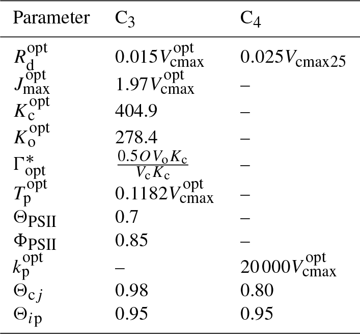
Download Print Version | Download XLSX

Appendix B: Temperature dependence of photosynthetic parameters

The photosynthesis model parameters for both the C₃ and C₄ pathways described in the previous section and shown in Table A1 have temperature-dependent variations and need to be adjusted for specific leaf temperature before implementing them in the photosynthesis model. The temperature dependence of photosynthetic parameters for the C₃ species can be broadly decomposed into two parts: (i) the temperature response and (ii) the high temperature inhibition. The functional form of these are as follows:

\begin{array}{l} f (T_{v}) = \exp [\frac{H_{a}}{R T_{0}} (1 - \frac{T_{0}}{T_{v}})], \\ (B1) & f_{H} (T_{v}) = \frac{1 + \exp (\frac{S_{v} T_{0} - H_{d}}{R T_{0}})}{1 + \exp (\frac{S_{v} T_{v} - H_{d}}{R T_{v}})}, \end{array}

where H_a is the activation energy, H_d is the deactivation energy, S_v is the entropy term, T₀ is the optimum temperature and T_v is the leaf temperature. The functional relationship of the different photosynthetic parameters in the C₃ pathway are as follows:

\begin{array}{l} V_{cmax} = V_{cmax}^{opt} f (T_{v}) f_{H} (T_{v}), \\ J_{\max} = J_{\max}^{opt} f (T_{v}) f_{H} (T_{v}), \\ T_{p} = T_{p}^{opt} f (T_{v}) f_{H} (T_{v}), \\ R_{d} = R_{d}^{opt} f (T_{v}) f_{H} (T_{v}), \\ K_{c} = K_{c}^{opt} f (T_{v}), \\ K_{o} = K_{o}^{opt} f (T_{v}), \\ (B2) & Γ^{*} = Γ_{opt}^{*} f (T_{v}) . \end{array}

The temperature dependence of photosynthetic parameters for the C₄ species are given by the following relationships:

\begin{array}{l} V_{cmax} = V_{cmax}^{opt} [\frac{f (Q_{10})}{f_{U} (T_{v}) f_{L} (T_{v})}], \\ f (Q_{10}) = Q_{10}^{(T_{v} - T_{0}) / 10}, \\ f_{U} (T_{v}) = 1 + \exp (s_{1} (T_{v} - s_{2})), \\ (B3) & f_{L} (T_{v}) = 1 + \exp (s_{3} (s_{4} - T_{v})), \end{array}

\begin{matrix} (B4) & R_{d} = R_{d}^{opt} [\frac{f (Q_{10})}{f_{U} (T_{v})}], \end{matrix}

\begin{matrix} (B5) & k_{p} = k_{p}^{opt} f (Q_{10}) . \end{matrix}

The Q₁₀ temperature coefficient is a measure of the rate of change of a biological or chemical system as a consequence of increasing the temperature by 10 ^∘C. The values of the temperature dependence functional parameters for both C₃ and C₄ species used in the present study are provided in Tables B1 and B2 respectively.

The temperature dependence parameters (activation, deactivation and entropy) are variable between different plant species (Leuning, 2002) as such its formulation in the newer implementation of the SCOPE model allows us to use appropriate values depending on the ecosystem we study.

A-g_s-C_i iterations

The final solution for photosynthesis requires an iterative solution of the coupled equations representing (i) the Farquhar, von Caemmerer and Berry (FvCB) model (Farquhar et al., 1980) for the photosynthesis rate (A); (ii) Fick's law of diffusion (Eq. B6) for internal (C_i) and leaf surface (C_s) CO₂ concentration; and (iii) Ball–Berry stomatal conductance model (Ball et al., 1987) (Eq. B7) for stomatal conductance (g_s) to obtain stable converging solutions.

\begin{matrix} (B6) & C_{i} = C_{s} - 1.6 \frac{A}{g_{s}} (from Fick's law), \end{matrix}

\begin{matrix} (B7) & g_{s} = g_{0} + {BB}_{slope} \frac{A r_{h}}{C_{s}} (Ball–Berry model). \end{matrix}

In Eq. (B7), BB_slope represents the Ball–Berry slope, r_h the relative humidity and g₀ the Ball–Berry intercept. In the absence of an initial specification of C_i, we make the assumption that g₀=0 in Eq. (B7); then, combining Eqs. (B6), (B7), the initial estimate of C_i is given as follows:

\begin{matrix} (B8) & C_{i} = \max (f_{C i}^{\min} C_{s}, C_{s} - 1.6 \frac{C_{s} r_{h}}{{BB}_{slope}}), \end{matrix}

where $f_{C i}^{\min}$ is the assumed minimum fractional leaf boundary layer CO₂ (assumed to be 0.3 for C₃ and 0.1 for C₄ species). This initial estimate of C_i is used to again estimate the photosynthesis based on the FvCB model (Farquhar et al., 1980), followed by estimation of stomatal conductance using the Ball–Berry model Eq. (B7). Finally, the Newton–Raphson method is used to obtain a forward estimation of the new value of internal CO₂ concentration (Ivanov et al., 2008; Sun et al., 2012). The updated C_i is further used in the A-g_s-C_i until convergence.

Table B1C₃ temperature dependence functional parameters.

Download Print Version | Download XLSX

Table B2C₄ temperature dependence functional parameters.

Download Print Version | Download XLSX

Appendix C: Derivation of iterative retrieval algorithm

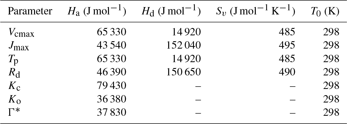
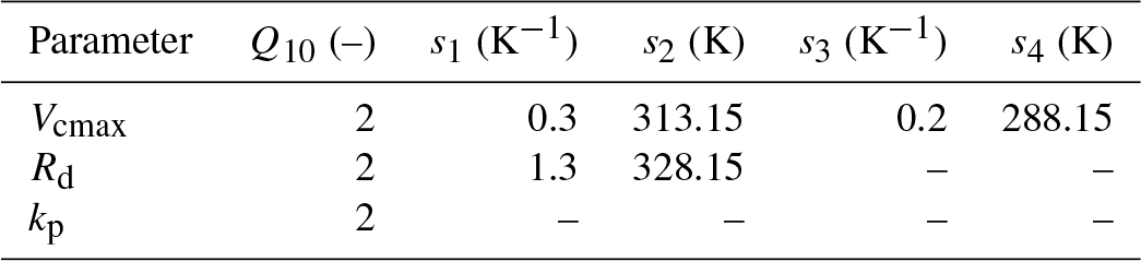
For deriving the maximum probability state X ( $\hat{X}$ ) we equate the derivative of the Eq. (5) to zero to obtain the following:

\begin{array}{l} \nabla_{X} {- 2 \ln P (X | Y)} & = - [\nabla_{X} F (X)]^{T} S_{ε}^{- 1} [Y - F (X)] \\ (C1) & + S_{a}^{- 1} [X - X_{a}] = 0 . \end{array}

It can be noted here that the gradient ∇_X of the above vector-valued function is a matrix-valued function and the Jacobian matrix is represented as K(X)=∇_XF(X), which results in the following implicit equation for $\hat{X}$ :

\begin{matrix} (C2) & - K^{T} (X) S_{ε}^{- 1} [Y - F (X)] + S_{a}^{- 1} [X - X_{a}] = 0 . \end{matrix}

We have to now use any general root-finding method for finding the solutions of Eq. (C2). If the problem is not too nonlinear we can use the Newton and Gauss–Newton iterative methods (Hartley, 1961). In general for any vector equation G(X)=0, we can write the Newton iteration as follows:

\begin{matrix} (C3) & X_{i + 1} = X_{i} - [\nabla_{X} G (X_{i})]^{- 1} G (X_{i}) . \end{matrix}

For our problem we can assume the derivative of the cost-function G(X) to be the left-hand side of Eq. (C1); therefore the gradient of G(X) (∇G) also known as the Hessian is given by the following:

\begin{array}{l} \nabla_{X} G (X) = \\ (C4) & S_{a}^{- 1} + K^{T} S_{ε}^{- 1} K - [\nabla_{X} K^{T}] S_{ε}^{- 1} [Y - F (X)] . \end{array}

The Hessian in Eq. (C4) involves the Jacobian K and both the first and second derivatives of the forward model. The second derivative is complicated because it is a vector whose elements are matrices and further this term is post-multiplied by the factor $S_{ε}^{- 1} [Y - F (X)]$ . The third term in the right-hand side of Eq. (C4) is thus computationally expensive and further for moderately linear problems this term is small; as such this term can be ignored (also called small-residual problems in numerical methods). When we ignore this term, we get the Gauss–Newton iteration scheme by substituting Eqs. (C2) and (C4) in Eq. (C3):

\begin{array}{l} X_{i + 1} & = X_{i} + (S_{a}^{- 1} + K_{i}^{T} S_{ε}^{- 1} K_{i})^{- 1} [K_{i}^{T} S_{ε}^{- 1} [Y - F (X_{i})] \\ (C5) & - S_{a}^{- 1} [X_{i} - X_{a}]], \end{array}

where K_i=K(X_i). We can substitute F(X) from Eq. (4) in Eq. (C2) to get the following:

\begin{array}{l} - K^{T} (\hat{X}) S_{ε}^{- 1} [Y - F (X)_{X = X_{l}} + \nabla_{X} F (X)_{X = X_{l}} (X - X_{l})] \\ (C6) & + S_{a}^{- 1} [\hat{X} - X_{a}] = 0 . \end{array}

Again, representing $K_{l} = \nabla_{X} F (X)_{X = X_{l}}$ , $F_{l} = F (X)_{X = X_{l}}$ we can further simplify and rearrange Eq. (C6) as follows:

\begin{array}{l} S_{a}^{- 1} [\hat{X} - X_{a}] + K_{l}^{T} S_{ε} K_{l} (\hat{X} - X_{a}) = \\ K_{l} S_{ε}^{- 1} [Y - F_{l} + K_{l} (X_{l} - X_{a})], \\ \hat{X} = X_{a} + (S_{a}^{- 1} + K_{l}^{T} S_{ε}^{- 1} K_{l})^{- 1} K_{l} S_{ε}^{- 1} [Y - F_{l} \\ (C7) & + K_{l} (X_{l} - X_{a})] . \end{array}

In the above equations, if we change the interpretation of the subscript l from “linearization” to “iteration counter”, we obtain the following equation:

\begin{array}{l} X_{i + 1} & = X_{a} + (S_{a}^{- 1} + K_{i}^{T} S_{ε}^{- 1} K_{i})^{- 1} K_{i} S_{ε}^{- 1} [Y - F (X_{i}) \\ (C8) & + K_{i} (X_{i} - X_{a})] . \end{array}

If we express X_i+1 as a departure from X_i rather than X_a we obtain the same expression for the iteration steps as Eqs. (C5) or (6).

Supplement

The supplement related to this article is available online at: https://doi.org/10.5194/bg-16-77-2019-supplement.

Author contributions

DD and CF designed the research, developed the inversion framework and conducted the modeling simulations. DD, CF, CvdT, YS and DSS contributed towards interpretation and analysis of the results. DD and CF developed the initial draft of the manuscript, and DD, CF, CvdT, YS and DSS contributed towards improvement of the original draft and finalization of the paper.

Competing interests

The authors declare that they have no conflict of interest.

Acknowledgements

AmeriFlux site Missouri Ozark (US-MOz) is supported by the US Department of Energy (DOE), Office of Science, Office of Biological and Environmental Research Program, through Oak Ridge National Laboratory's Terrestrial Ecosystem Science-Science Focus Area; ORNL is managed by UT-Battelle, LLC, for DOE under contract DE-AC05-00OR22725.

The research was carried out, in part, at the Jet Propulsion Laboratory, California Institute of Technology, under a contract with the National Aeronautics and Space Administration. Government sponsorship is acknowledged.

Edited by: Dan Yakir
Reviewed by: Peter Rayner and two anonymous referees

References

Baldocchi, D.: An analytical solution for coupled leaf photosynthesis and stomatal conductance models, Tree Physiol., 14, 1069–1079, 1994. a

Baldocchi, D., Valentini, R., Running, S., Oechel, W., and Dahlman, R.: Strategies for measuring and modelling carbon dioxide and water vapour fluxes over terrestrial ecosystems, Glob. Change Biol., 2, 159–168, 1996. a

Baldocchi, D., Kelliher, F. M., Black, T. A., and Jarvis, P.: Climate and vegetation controls on boreal zone energy exchange, Glob. Change Biol., 6, 69–83, 2000. a

Baldocchi, D., Falge, E., Gu, L., Olson, R., Hollinger, D., Running, S., Anthoni, P., Bernhofer, C., Davis, K., Evans, R., et al.: FLUXNET: A new tool to study the temporal and spatial variability of ecosystem–scale carbon dioxide, water vapor, and energy flux densities, B. Am. Meteorol. Soc., 82, 2415–2434, 2001. a

Ball, J. T., Woodrow, I. E., and Berry, J. A.: A model predicting stomatal conductance and its contribution to the control of photosynthesis under different environmental conditions, Progress in photosynthesis research, 221–224, Springer, Dordrecht, 1987. a, b

Beerling, D. and Quick, W.: A new technique for estimating rates of carboxylation and electron transport in leaves of C3 plants for use in dynamic global vegetation models, Glob. Change Biol., 1, 289–294, 1995. a

Bernacchi, C. J., Singsaas, E. L., Pimentel, C., Portis Jr., A. R., and Long, S. P.: Improved temperature response functions for models of Rubisco-limited photosynthesis, Plant Cell Environ., 24, 253–259, 2001. a, b

Bonan, G. B., Lawrence, P. J., Oleson, K. W., Levis, S., Jung, M., Reichstein, M., Lawrence, D. M., and Swenson, S. C.: Improving canopy processes in the Community Land Model version 4 (CLM4) using global flux fields empirically inferred from FLUXNET data, J. Geophys. Res.-Biogeo., 116, https://doi.org/10.1029/2010JG001593, 2011. a, b, c, d

Burns, S. P., Maclean, G. D., Blanken, P. D., Oncley, S. P., Semmer, S. R., and Monson, R. K.: The Niwot Ridge Subalpine Forest US-NR1 AmeriFlux site – Part 1: Data acquisition and site record-keeping, Geosci. Instrum. Method. Data Syst., 5, 451–471, https://doi.org/10.5194/gi-5-451-2016, 2016. a

Chen, J. M., Rich, P. M., Gower, S. T., Norman, J. M., and Plummer, S.: Leaf area index of boreal forests: Theory, techniques, and measurements, J. Geophys. Res.-Atmos., 102, 29429–29443, 1997. a, b

Collatz, G., Ball, J., Grivet, C., and Berry, J. A.: Physiological and environmental regulation of stomatal conductance, photosynthesis and transpiration: a model that includes a laminar boundary layer, Agr. Forest Meteorol., 54, 107–136, https://doi.org/10.1016/0168-1923(91)90002-8, 1991a. a

Collatz, G. J., Ball, J. T., Grivet, C., and Berry, J. A.: Physiological and environmental regulation of stomatal conductance, photosynthesis and transpiration: a model that includes a laminar boundary layer, Agr. Forest Meteorol., 54, 107–136, 1991b. a

Collatz, G. J., Ribas-Carbo, M., and Berry, J.: Coupled photosynthesis-stomatal conductance model for leaves of C4 plants, Funct. Plant Biol., 19, 519–538, 1992. a, b

Cox, P. M., Pearson, D., Booth, B. B., Friedlingstein, P., Huntingford, C., Jones, C. D., and Luke, C. M.: Sensitivity of tropical carbon to climate change constrained by carbon dioxide variability, Nature, 494, p. 341, 2013. a

Cramer, W., Bondeau, A., Woodward, F. I., Prentice, I. C., Betts, R. A., Brovkin, V., Cox, P. M., Fisher, V., Foley, J. A., Friend, A. D., et al.: Global response of terrestrial ecosystem structure and function to CO₂ and climate change: results from six dynamic global vegetation models, Glob. Change Biol., 7, 357–373, 2001. a

Dai, Y., Dickinson, R. E., and Wang, Y.-P.: A two-big-leaf model for canopy temperature, photosynthesis, and stomatal conductance, J. Climate, 17, 2281–2299, 2004. a

Dutta, D., Wang, K., Lee, E., Goodwell, A., Woo, D. K., Wagner, D., and Kumar, P.: Characterizing Vegetation Canopy Structure Using Airborne Remote Sensing Data, IEEE T. Geosci. Remote, 55, 1160–1178, 2017. a, b

Falkowski, P., Scholes, R. J., Boyle, E. E. A., Canadell, J., Canfield, D., Elser, J., Gruber, N., Hibbard, K., Högberg, P., Linder, S., and Mackenzie, F. T.: The global carbon cycle: a test of our knowledge of earth as a system, Science, 290, 291–296, 2000. a

Farquhar, G. v., von Caemmerer, S. V., and Berry, J.: A biochemical model of photosynthetic CO₂ assimilation in leaves of C3 species, Planta, 149, 78–90, 1980. a, b, c, d, e

Flexas, J., Escalona, J. M., Evain, S., Gulías, J., Moya, I., Osmond, C. B., and Medrano, H.: Steady-state chlorophyll fluorescence (Fs) measurements as a tool to follow variations of net CO₂ assimilation and stomatal conductance during water-stress in C3 plants, Physiol. Plantarum, 114, 231–240, 2002. a

FLUXNET community: FLUXNET 2015 dataset, available at: http://fluxnet.fluxdata.org/data/fluxnet2015-dataset/, last access: 26 October 2015.

Frankenberg, C., Fisher, J. B., Worden, J., Badgley, G., Saatchi, S. S., Lee, J. E., Toon, G. C., Butz, A., Jung, M., Kuze, A., and Yokota, T.: New global observations of the terrestrial carbon cycle from GOSAT: Patterns of plant fluorescence with gross primary productivity, Geophys. Res. Lett., 38, https://doi.org/10.1029/2011GL048738, 2011. a, b

Frankenberg, C., O'Dell, C., Berry, J., Guanter, L., Joiner, J., Köhler, P., Pollock, R., and Taylor, T. E.: Prospects for chlorophyll fluorescence remote sensing from the Orbiting Carbon Observatory-2, Remote Sens. Environ., 147, 1–12, 2014. a

Frankenberg, C., Drewry, D., Geier, S., Verma, M., Lawson, P., Stutz, J., and Grossmann, K.: Remote sensing of solar induced Chlorophyll Fluorescence from satellites, airplanes and ground-based stations, in: Geoscience and Remote Sensing Symposium (IGARSS), 2016 IEEE International, 1707–1710, IEEE, 2016. a

Friedlingstein, P., Cox, P., Betts, R., Bopp, L., von Bloh, W., Brovkin, V., Cadule, P., Doney, S., Eby, M., Fung, I., and Bala, G.: Climate–carbon cycle feedback analysis: results from the C4MIP model intercomparison, J. Climate, 19, 3337–3353, 2006. a

Gu, L., Meyers, T., Pallardy, S. G., Hanson, P. J., Yang, B., Heuer, M., Hosman, K. P., Riggs, J. S., Sluss, D., and Wullschleger, S. D.: Direct and indirect effects of atmospheric conditions and soil moisture on surface energy partitioning revealed by a prolonged drought at a temperate forest site, J. Geophys. Res.-Atmos., 111, https://doi.org/10.1029/2006JD007161, 2006. a

Guanter, L., Zhang, Y., Jung, M., Joiner, J., Voigt, M., Berry, J. A., Frankenberg, C., Huete, A. R., Zarco-Tejada, P., Lee, J. E., and Moran, M. S.: Global and time-resolved monitoring of crop photosynthesis with chlorophyll fluorescence, P. Natl. Acad. Sci. USA, 111, E1327–E1333, 2014. a

Han, Q., Kawasaki, T., Nakano, T., and Chiba, Y.: Spatial and seasonal variability of temperature responses of biochemical photosynthesis parameters and leaf nitrogen content within a Pinus densiflora crown, Tree Physiol., 24, 737–744, 2004. a

Hartley, H. O.: The modified Gauss-Newton method for the fitting of non-linear regression functions by least squares, Technometrics, 3, 269–280, 1961. a

Heimann, M. and Reichstein, M.: Terrestrial ecosystem carbon dynamics and climate feedbacks, Nature, 451, 7176, https://doi.org/10.1038/nature06591, 2008. a

Houborg, R., Soegaard, H., and Boegh, E.: Combining vegetation index and model inversion methods for the extraction of key vegetation biophysical parameters using Terra and Aqua MODIS reflectance data, Remote Sens. Environ., 106, 39–58, 2007. a

Ivanov, V. Y., Bras, R. L., and Vivoni, E. R.: Vegetation-hydrology dynamics in complex terrain of semiarid areas: 1. A mechanistic approach to modeling dynamic feedbacks, Water Resour. Res., 44, https://doi.org/10.1029/2006WR005588, 2008. a

Jacquemoud, S., Baret, F., Andrieu, B., Danson, F., and Jaggard, K.: Extraction of vegetation biophysical parameters by inversion of the PROSPECT+ SAIL models on sugar beet canopy reflectance data. Application to TM and AVIRIS sensors, Remote Sens. Environ., 52, 163–172, 1995. a

Katul, G., Manzoni, S., Palmroth, S., and Oren, R.: A stomatal optimization theory to describe the effects of atmospheric CO₂ on leaf photosynthesis and transpiration, Ann. Bot.-London, 105, 431–442, 2009. a

Knorr, W. and Heimann, M.: Uncertainties in global terrestrial biosphere modeling: 1. A comprehensive sensitivity analysis with a new photosynthesis and energy balance scheme, Global Biogeochem. Cy., 15, 207–225, 2001. a

Knorr, W. and Kattge, J.: Inversion of terrestrial ecosystem model parameter values against eddy covariance measurements by Monte Carlo sampling, Glob. Change Biol., 11, 1333–1351, 2005. a

Kucharik, C. J., Foley, J. A., Delire, C., Fisher, V. A., Coe, M. T., Lenters, J. D., Young-Molling, C., Ramankutty, N., Norman, J. M., and Gower, S. T.: Testing the performance of a dynamic global ecosystem model: water balance, carbon balance, and vegetation structure, Global Biogeochem. Cy., 14, 795–825, 2000. a

Lawrence, D. M., Oleson, K. W., Flanner, M. G., Thornton, P. E., Swenson, S. C., Lawrence, P. J., Zeng, X., Yang, Z. L., Levis, S., Sakaguchi, K., and Bonan, G. B.: Parameterization improvements and functional and structural advances in version 4 of the Community Land Model, J. Adv. Model. Earth Sy., 3, https://doi.org/10.1029/2011MS00045, 2011. a

Leuning, R.: Temperature dependence of two parameters in a photosynthesis model, Plant Cell Environ., 25, 1205–1210, 2002. a, b, c, d, e

Leuning, R., Van Gorsel, E., Massman, W. J., and Isaac, P. R.: Reflections on the surface energy imbalance problem, Agr. Forest Meteorol., 156, 65–74, 2012. a

Levenberg, K.: A method for the solution of certain non-linear problems in least squares, Q. Appl. Math., 2, 164–168, 1944. a

Liu, J., Bowman, K. W., Schimel, D. S., Parazoo, N. C., Jiang, Z., Lee, M., Bloom, A. A., Wunch, D., Frankenberg, C., Sun, Y., and O'Dell, C. W.: Contrasting carbon cycle responses of the tropical continents to the 2015–2016 El Niño, Science, 358, 6360, https://doi.org/10.1126/science.aam5690, 2017. a

Mackay, D. S., Ewers, B. E., Loranty, M. M., Kruger, E. L., and Samanta, S.: Bayesian analysis of canopy transpiration models: a test of posterior parameter means against measurements, J. Hydrol., 432, 75–83, 2012. a

Mäkelä, A., Berninger, F., and Hari, P.: Optimal control of gas exchange during drought: theoretical analysis, Ann. Bot.-London, 77, 461–468, 1996. a

Marquardt, D. W.: An algorithm for least-squares estimation of nonlinear parameters, J. Soc. Ind. Appl. Math., 11, 431–441, 1963. a, b

McGuire, A. D., Sitch, S., Clein, J. S., Dargaville, R., Esser, G., Foley, J., Heimann, M., Joos, F., Kaplan, J., Kicklighter, D. W., and Meier, R. A.: Carbon balance of the terrestrial biosphere in the twentieth century: Analyses of CO₂, climate and land use effects with four process-based ecosystem models, Global Biogeochem. Cy., 15, 183–206, 2001. a

McGuire, A., Wirth, C., Apps, M., Beringer, J., Clein, J., Epstein, H., Kicklighter, D., Bhatti, J., Chapin, F., Groot, B., Efremov, D., Eugster, W., Fukuda, M., Gower, T., Hinzman, L., Huntley, B., Jia, G., Kasischke, E., Melillo, J., Romanovsky, V., Shvidenko, A., Vaganov, E., and Walker, D.: Environmental variation, vegetation distribution, carbon dynamics and water/energy exchange at high latitudes, J. Veg. Sci., 13, 301–314, 2002. a

Medlyn, B. E., Duursma, R. A., Eamus, D., Ellsworth, D. S., Prentice, I. C., Barton, C. V., Crous, K. Y., De Angelis, P., Freeman, M., and Wingate, L.: Reconciling the optimal and empirical approaches to modelling stomatal conductance, Glob. Change Biol., 17, 2134–2144, 2011. a

Monson, R., Turnipseed, A., Sparks, J., Harley, P., Scott-Denton, L., Sparks, K., and Huxman, T.: Carbon sequestration in a high-elevation, subalpine forest, Glob. Change Biol., 8, 459–478, 2002. a

Monson, R. K., Prater, M. R., Hu, J., Burns, S. P., Sparks, J. P., Sparks, K. L., and Scott-Denton, L. E.: Tree species effects on ecosystem water-use efficiency in a high-elevation, subalpine forest, Oecologia, 162, 491–504, 2009. a

Monteith, J. and Unsworth, M.: Principles of environmental physics, Academic Press, USA, 2007. a

Myneni, R. B., Ramakrishna, R., Nemani, R., and Running, S. W.: Estimation of global leaf area index and absorbed PAR using radiative transfer models, IEEE T. Geosci. Remote, 35, 1380–1393, 1997. a

Oleson, K., Lawrence, D., Bonan, G., Drewniak, B., Huang, M., Koven, C., Levis, S., Li, F., Riley, W., Subin, Z., and Swenson, S.: Technical description of version 4.5 of the Community Land Model (CLM), 420 pp., 2013. a

Oleson, K. W., Lawrence, D. M., Gordon, B., Flanner, M. G., Kluzek, E., Peter, J., Levis, S., Swenson, S. C., Thornton, E., Feddema, J., and Heald, C. L.: Technical description of version 4.0 of the Community Land Model (CLM), 2010. a

Pappas, C., Fatichi, S., Leuzinger, S., Wolf, A., and Burlando, P.: Sensitivity analysis of a process-based ecosystem model: Pinpointing parameterization and structural issues, J. Geophys. Res.-Biogeo., 118, 505–528, 2013. a

Quaife, T., Lewis, P., De Kauwe, M., Williams, M., Law, B. E., Disney, M., and Bowyer, P.: Assimilating canopy reflectance data into an ecosystem model with an Ensemble Kalman Filter, Remote Sens. Environ., 112, 1347–1364, 2008. a

Reed, D. E., Frank, J. M., Ewers, B. E., and Desai, A. R.: Time dependency of eddy covariance site energy balance, Agr. Forest Meteorol., 249, 467–478, 2018. a

Reichstein, M., Rey, A., Freibauer, A., Tenhunen, J., Valentini, R., Banza, J., Casals, P., Cheng, Y., Grünzweig, J. M., Irvine, J., and Joffre, R.: Modeling temporal and large-scale spatial variability of soil respiration from soil water availability, temperature and vegetation productivity indices, Global Biogeochem. Cy., 17, https://doi.org/10.1029/2003GB002035, 2003. a

Ricciuto, D. M., Davis, K. J., and Keller, K.: A Bayesian calibration of a simple carbon cycle model: The role of observations in estimating and reducing uncertainty, Global Biogeochem. Cy., 22, https://doi.org/10.1029/2006GB002908, 2008. a

Rodgers, C. D.: Inverse methods for atmospheric sounding: theory and practice, vol. 2, World scientific, 2000. a, b, c, d

Rogers, A., Medlyn, B. E., Dukes, J. S., Bonan, G., Caemmerer, S., Dietze, M. C., Kattge, J., Leakey, A. D., Mercado, L. M., Niinemets, Ü., and Prentice, I. C.: A roadmap for improving the representation of photosynthesis in Earth system models, New Phytol., 213, 22–42, 2017. a

Running, S. W. and Coughlan, J. C.: A general model of forest ecosystem processes for regional applications I. Hydrologic balance, canopy gas exchange and primary production processes, Ecol. Model., 42, 125–154, 1988. a

Sánchez, J. M., Caselles, V., and Rubio, E. M.: Analysis of the energy balance closure over a FLUXNET boreal forest in Finland, Hydrol. Earth Syst. Sci., 14, 1487–1497, https://doi.org/10.5194/hess-14-1487-2010, 2010. a

Schaaf, C. and Wang, Z.: MCD43A4 MODIS/Terra+ Aqua BRDF/Albedo Nadir BRDF Adjusted RefDaily L3 Global 500 m V006, NASA EOSDIS Land Processes DAAC, available at: https://doi.org/10.5067/MODIS/MCD43A4.006, 2015. a

Schimel, D. S.: Terrestrial ecosystems and the carbon cycle, Glob. Change Biol., 1, 77–91, 1995. a

Schulze, E., Kelliher, F. M., Korner, C., Lloyd, J., and Leuning, R.: Relationships among maximum stomatal conductance, ecosystem surface conductance, carbon assimilation rate, and plant nitrogen nutrition: a global ecology scaling exercise, Annu. Rev. Ecol. Syst., 25, 629–662, 1994. a

Simioni, G., Gignoux, J., Le Roux, X., Appé, R., and Benest, D.: Spatial and temporal variations in leaf area index, specific leaf area and leaf nitrogen of two co-occurring savanna tree species, Tree Physiol., 24, 205–216, 2004. a

Sitch, S., Smith, B., Prentice, I. C., Arneth, A., Bondeau, A., Cramer, W., Kaplan, J. O., Levis, S., Lucht, W., Sykes, M. T., and Thonicke, K.: Evaluation of ecosystem dynamics, plant geography and terrestrial carbon cycling in the LPJ dynamic global vegetation model, Glob. Change Biol., 9, 161–185, 2003. a, b

Sitch, S., Huntingford, C., Gedney, N., Levy, P. E., Lomas, M., Piao, S. L., Betts, R., Ciais, P., Cox, P., Friedlingstein, P., and Jones, C. D.: Evaluation of the terrestrial carbon cycle, future plant geography and climate-carbon cycle feedbacks using five Dynamic Global Vegetation Models (DGVMs), Glob. Change Biol., 14, 2015–2039, 2008. a

Sitch, S., Friedlingstein, P., Gruber, N., Jones, S. D., Murray-Tortarolo, G., Ahlström, A., Doney, S. C., Graven, H., Heinze, C., Huntingford, C., Levis, S., Levy, P. E., Lomas, M., Poulter, B., Viovy, N., Zaehle, S., Zeng, N., Arneth, A., Bonan, G., Bopp, L., Canadell, J. G., Chevallier, F., Ciais, P., Ellis, R., Gloor, M., Peylin, P., Piao, S. L., Le Quéré, C., Smith, B., Zhu, Z., and Myneni, R.: Recent trends and drivers of regional sources and sinks of carbon dioxide, Biogeosciences, 12, 653–679, https://doi.org/10.5194/bg-12-653-2015, 2015. a

Sun, Y., Gu, L., and Dickinson, R. E.: A numerical issue in calculating the coupled carbon and water fluxes in a climate model, J. Geophys. Res., 117, https://doi.org/10.1029/2012JD018059, 2012. a, b, c

Suyker, A. E., Verma, S. B., Burba, G. G., and Arkebauer, T. J.: Gross primary production and ecosystem respiration of irrigated maize and irrigated soybean during a growing season, Agr. Forest Meteorol., 131, 180–190, 2005. a

Tanaka, K., Kosugi, Y., and Nakamura, A.: Impact of leaf physiological characteristics on seasonal variation in CO₂, latent and sensible heat exchanges over a tree plantation, Agr. Forest Meteorol., 114, 103–122, 2002. a, b

Tuzet, A., Perrier, A., and Leuning, R.: A coupled model of stomatal conductance, photosynthesis and transpiration, Plant Cell Environ., 26, 1097–1116, 2003. a

van der Tol, C.: SCOPE model, available at: https://github.com/Christiaanvandertol/SCOPE, last access: 28 August 2017.

Van der Tol, C., Dolman, A., Waterloo, M., and Meesters, A.: Optimum vegetation characteristics, assimilation, and transpiration during a dry season: 2. Model evaluation, Water Resour. Res., 44, https://doi.org/10.1029/2007WR006243, 2008a. a

Van der Tol, C., Meesters, A., Dolman, A., and Waterloo, M.: Optimum vegetation characteristics, assimilation, and transpiration during a dry season: 1. Model description, Water Resour. Res., 44, https://doi.org/10.1029/2007WR006241, 2008b. a

van der Tol, C., Verhoef, W., Timmermans, J., Verhoef, A., and Su, Z.: An integrated model of soil-canopy spectral radiances, photosynthesis, fluorescence, temperature and energy balance, Biogeosciences, 6, 3109–3129, https://doi.org/10.5194/bg-6-3109-2009, 2009. a, b, c, d, e

Verhoef, W., Jia, L., Xiao, Q., and Su, Z.: Unified optical-thermal four-stream radiative transfer theory for homogeneous vegetation canopies, IEEE T. Geosci. Remote, 45, 1808–1822, 2007. a

von Randow, C., Manzi, A. O., Kruijt, B., De Oliveira, P. J., Zanchi, F. B., Silva, R. L., Hodnett, M. G., Gash, J. H. C., Elbers, J. A., Waterloo, M. J., and Cardoso, F. L.: Comparative measurements and seasonal variations in energy and carbon exchange over forest and pasture in South West Amazonia, Theor. Appl. Climatol., 78, 5–26, 2004. a

Wang, Q., Iio, A., Tenhunen, J., and Kakubari, Y.: Annual and seasonal variations in photosynthetic capacity of Fagus crenata along an elevation gradient in the Naeba Mountains, Japan, Tree Physiol., 28, 277–285, 2008. a

Wang, Y.-P. and Leuning, R.: A two-leaf model for canopy conductance, photosynthesis and partitioning of available energy I:: Model description and comparison with a multi-layered model, Agr. Forest Meteorol., 91, 89–111, 1998. a

Wilson, K., Goldstein, A., Falge, E., Aubinet, M., Baldocchi, D., Berbigier, P., Bernhofer, C., Ceulemans, R., Dolman, H., Field, C., and Grelle, A.: Energy balance closure at FLUXNET sites, Agr. Forest Meteorol., 113, 223–243, 2002. a

Wilson, K. B. and Baldocchi, D. D.: Seasonal and interannual variability of energy fluxes over a broadleaved temperate deciduous forest in North America, Agr. Forest Meteorol., 100, 1–18, 2000. a

Wilson, K. B., Baldocchi, D. D., and Hanson, P. J.: Spatial and seasonal variability of photosynthetic parameters and their relationship to leaf nitrogen in a deciduous forest, Tree Physiol., 20, 565–578, 2000. a, b, c, d, e

Wolf, A., Akshalov, K., Saliendra, N., Johnson, D. A., and Laca, E. A.: Inverse estimation of Vc max, leaf area index, and the Ball-Berry parameter from carbon and energy fluxes, J. Geophys. Res., 111, 1–18, 2006. a, b, c

Wramneby, A., Smith, B., Zaehle, S., and Sykes, M. T.: Parameter uncertainties in the modelling of vegetation dynamics?effects on tree community structure and ecosystem functioning in European forest biomes, Ecol. Model., 216, 277–290, 2008. a

Wu, X., Luo, Y., Weng, E., White, L., Ma, Y., and Zhou, X.: Conditional inversion to estimate parameters from eddy-flux observations, J. Plant Ecol., 2, 55–68, 2009. a

Wullschleger, S. D.: Biochemical limitations to carbon assimilation in C3 plants – a retrospective analysis of the A/Ci curves from 109 species, J. Exp. Bot., 44, 907–920, 1993. a, b

Xu, L. and Baldocchi, D. D.: Seasonal trends in photosynthetic parameters and stomatal conductance of blue oak (Quercus douglasii) under prolonged summer drought and high temperature, Tree Physiol., 23, 865–877, 2003. a, b

Xu, T., White, L., Hui, D., and Luo, Y.: Probabilistic inversion of a terrestrial ecosystem model: Analysis of uncertainty in parameter estimation and model prediction, Global Biogeochem. Cy., 20, https://doi.org/10.1029/2005GB002468, 2006. a

Zaehle, S., Sitch, S., Smith, B., and Hatterman, F.: Effects of parameter uncertainties on the modeling of terrestrial biosphere dynamics, Global Biogeochem. Cy., 19, https://doi.org/10.1029/2004GB002395, 2005. a

Optimal inverse estimation of ecosystem parameters from observations of carbon and energy fluxes

2.1 The SCOPE biochemical module

2.2 Comparison of current and previous photosynthesis implementations in SCOPE

5.1 Levenberg–Marquardt method

5.2 A moving window setup of the inversion problem using flux tower observations

5.3 Error characterization and convergence criteria for the retrievals

6.1 Data filtering criteria in the moving window retrievals

6.2 MODIS satellite reflectance data

6.3 Retrieval results for the Nebraska Mead-1 site

6.3.1 Site description

6.3.2 Inversion parameters and results

6.4 Retrieval results for the Missouri Ozark site

6.4.1 Site description

6.4.2 Inversion parameters and results for the year 2009

6.4.3 Inversion results for the year 2007

6.5 Retrieval results for the Niwot Ridge site

6.5.1 Site description

6.5.2 Inversion parameters and results

A-gs-Ci iterations

A-g_s-C_i iterations