the Creative Commons Attribution 4.0 License.
the Creative Commons Attribution 4.0 License.
 | 01 Feb 2019
High-frequency variability of CO2 in Grand Passage, Bay of Fundy, Nova Scotia
Alex E. Hay
William J. Burt
Richard A. Cheel
Joseph Salisbury
Helmuth Thomas
Assessing changes in the marine carbon cycle arising from anthropogenic CO2 emissions requires a detailed understanding of the carbonate system's natural variability. Coastal ecosystems vary over short spatial and temporal scales, so their dynamics are not well described by long-term and broad regional averages. A year-long time series of pCO2, temperature, salinity, and currents is used to quantify the high-frequency variability of the carbonate system at the mouth of the Bay of Fundy, Nova Scotia. The seasonal cycle of pCO2 is modulated by a diel cycle that is larger in summer than in winter and a tidal contribution that is primarily M2, with amplitude roughly half that of the diel cycle throughout the year. The interaction between tidal currents and carbonate system variables leads to lateral transport by tidal pumping, which moves alkalinity and dissolved inorganic carbon (DIC) out of the bay, opposite to the mean flow in the region, and constitutes a new feature of how this strongly tidal region connects to the larger Gulf of Maine and northwest Atlantic carbon system. These results suggest that tidal pumping could substantially modulate the coastal ocean's response to global ocean acidification in any region with large tides and spatial variation in biological activity, requiring that high-frequency variability be accounted for in assessments of carbon budgets of coastal regions.


Oceanic uptake of anthropogenic carbon dioxide (CO2) moderates the rise of atmospheric CO2 concentrations and leads to changes in the ocean carbon cycle. CO2 uptake acidifies the oceans, potentially altering ecosystems and leading to adverse effects for the societies and industries that depend on them. Assessing the vulnerability of these resources to long-term change in ocean acidification requires a detailed understanding of the carbonate system's natural variability that any anthropogenic trend may add to or alter. Coastal ecosystems vary on shorter temporal and spatial scales than the shelf or open ocean so predicting how they may change under future climate scenarios is more difficult and requires an understanding of the system's high-frequency components.
The Bay of Fundy (Fig. 1, inset) is an approximately 200 km long, 50 km wide, 75 m deep bay that extends northeastward into Canada from the Gulf of Maine in the northwest Atlantic Ocean. The regional circulation flows southward along the Scotian Shelf as the Nova Scotia Current, follows the coastline around southern Nova Scotia to enter the southern side of the Bay of Fundy, and exits the bay along the northern side to join the Eastern Maine Coastal Current in the Gulf of Maine (Bigelow, 1927; Greenberg, 1983; Hannah et al., 2001; Pettigrew et al., 2005; Dever et al., 2016). The mean circulation and water properties of the Gulf of Maine and the Nova Scotia Current are well described (e.g., Smith, 1989; Smith et al., 2001; Hannah et al., 2001; Houghton and Fairbanks, 2001; Aretxabaleta et al., 2008; Gledhill et al., 2015; Dever et al., 2016). Within the bay the mean flow recirculates cyclonically around the outer Bay of Fundy (Aretxabaleta et al., 2008). The geometry of the basin makes it resonant with the M2 tidal frequency and generates the highest tidal range in the world, over 16 m at the head of the bay (Garrett, 1972; Greenberg, 1983). Turbulence from the fast tidal flows keeps much of the basin well mixed, while the deeper regions of the outer bay develop seasonal stratification. The largest freshwater source to the bay is the St. John River, on the northern coast, so owing to river plume dynamics and the general circulation of the region, this river water primarily propagates along the northern coast, into the Gulf of Maine.
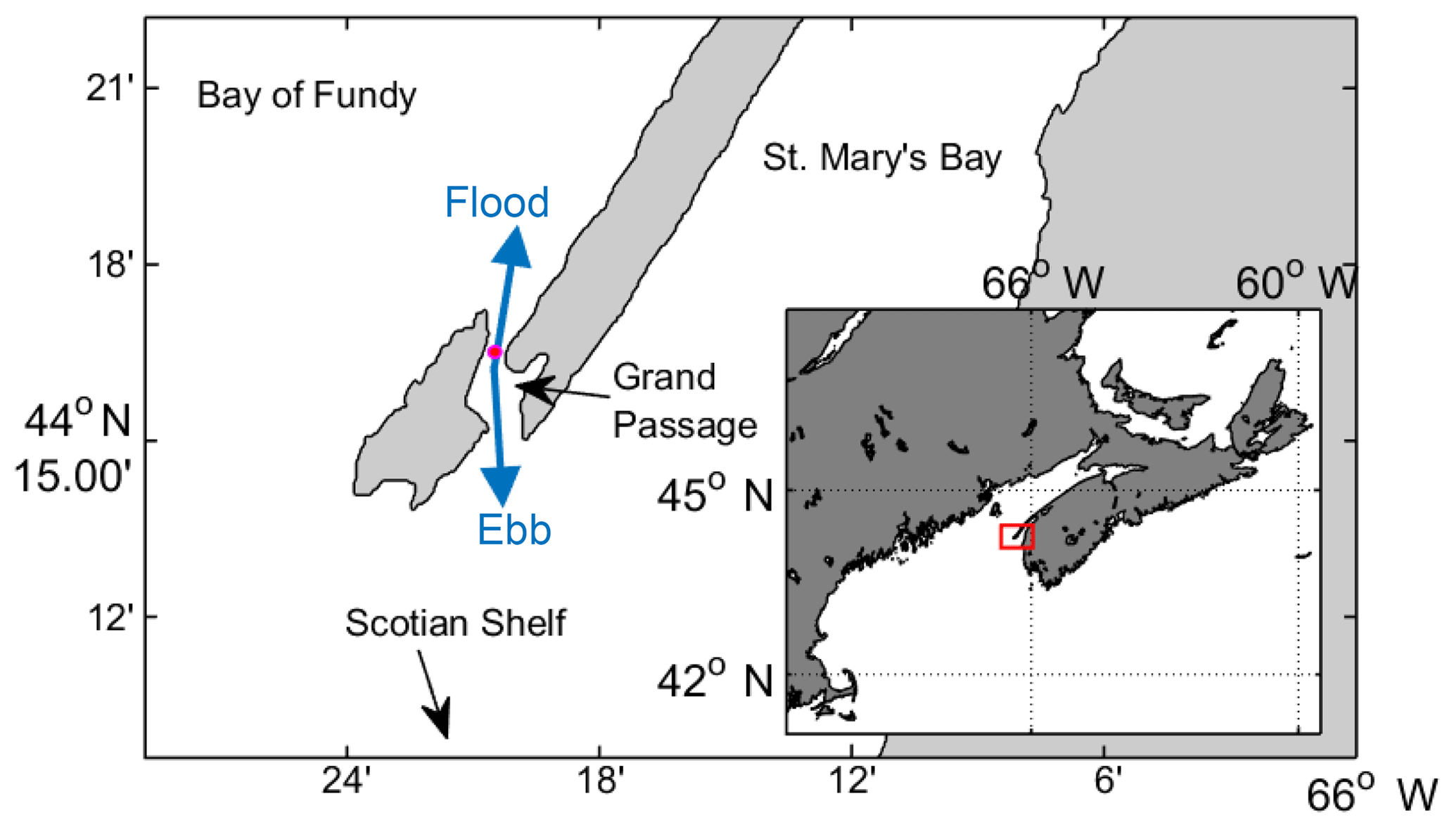
Figure 1Map of Grand Passage, which cuts through a peninsula in southwest Nova Scotia. Instrument location indicated by the pink dot. Flood and ebb tide flow directions shown in blue arrows. Inset: map of the region with the red box indicating the field site at the mouth of the Bay of Fundy.
Seasonal and inter-annual variability in air–sea CO2 flux, along with the key carbon cycling processes, have been documented both upstream from the Bay of Fundy on the Scotian Shelf (e.g., Shadwick et al., 2010, 2011; Thomas et al., 2012; Craig et al., 2015) and downstream in the Gulf of Maine (Salisbury et al., 2009; Vandemark et al., 2011). Within the bay, salt marshes have been shown to be weak emitters of CO2 to the atmosphere (Magenheimer et al., 1996), but these results might not be representative of fully submerged regions. Basin-wide estimates of CO2 fluxes have come as part of larger-scale coastal studies where the Bay of Fundy is included as part of the Gulf of Maine region. Using historical pCO2 data and satellite algorithms, Signorini et al. (2013) identified the Gulf of Maine as a weak source of CO2 to the atmosphere. In contrast, results from a coupled biogeochemical-circulation model indicate the Gulf of Maine to be a relatively strong sink of CO2 compared to surrounding areas (Cahill et al., 2016).
The coastal carbon budget and thus the rate at which alkalinity will be able to buffer future ocean acidification depend on the exchange processes between coastal and open oceans. In shallow marshy estuaries, tidal budgets have been estimated for oxygen from dissolved oxygen measurements (Nidzieko et al., 2014) and for carbon from a linear model based on pH and oxidation-reduction potential (Wang et al., 2016). However, to the best of our knowledge, the tidal transport of carbon in this macrotidal system, or far from large freshwater or nutrient sources, has never been addressed.
To investigate this issue, a year-long, high-frequency time series of pCO2, temperature, salinity, and currents was measured via a cabled-to-shore platform in Grand Passage, a tidal channel at the mouth of the Bay of Fundy, Nova Scotia (Fig. 1). This location is ideal for tracing the main input of water into the Bay from the Scotian Shelf. We quantify carbonate system variability on hourly to seasonal timescales, unravel the interaction between the daily and tidal cycles, determine the phase relationship between tidal currents and carbonate system variables, and estimate lateral transports by tidal pumping, which moves alkalinity and dissolved inorganic carbon (DIC) out of the bay, opposite to the mean flow in the region.
Grand Passage is a narrow channel (1 km wide, 4 km long) separating Brier Island from Long Island at the end of the Digby Neck peninsula, which juts out into the mouth of the Bay of Fundy from the southwest corner of Nova Scotia (Fig. 1, inset). The tidal range is 5 to 6 m and peak tidal velocities range from 2 to 3 m s−1.
2.1 Time series measurements
A year-long record of high-frequency measurements of pCO2 (Fig. 2a), temperature (Fig. 2b), and pressure, 4 months of salinity (Fig. 2c), and 1 month of velocity data were collected via a cabled-to-shore observatory on a bottom frame that was deployed in approximately 10.5 m mean water depth (location indicated on Fig. 1).
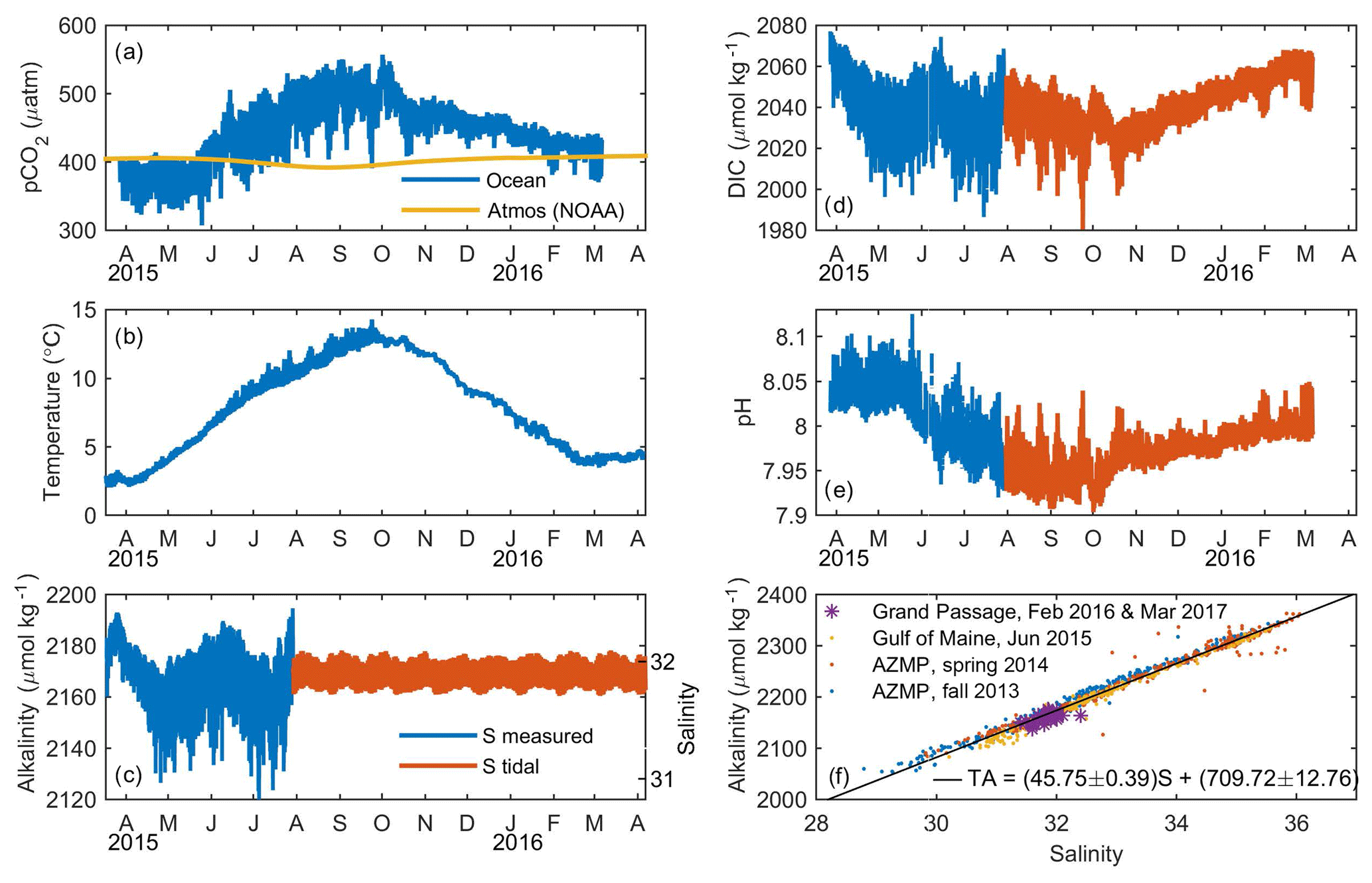
Figure 2(a–c) Measured variables and (d, e) time series generated from the carbonate system equilibrium solution for data shown in (a–c). (a) pCO2 in Grand Passage (blue) and NOAA's weekly atmospheric zonal average for 44–45∘ N (yellow). (b) Temperature. (c) Salinity (right y axis) and alkalinity (left y axis) from periods with salinity data (blue) and generated from a tidal prediction when measurements were not available owing to instrument failure (orange). (d) DIC. (e) pH. (f) Alkalinity vs. salinity from bottle samples at the Grand Passage field site in 2016 and 2017 (purple) as well as from the Scotian Shelf via the Atlantic Zone Monitoring Program (AZMP) in 2013 (blue) and 2014 (orange) and the Gulf of Maine in 2015 (yellow). Linear regression (black) used to generate alkalinity shown in (c).
The primary instrument for this experiment was a CONTROS HydroC CO2 sensor, which uses non-dispersive infrared spectrometry (NDIR) to measure gas concentrations that have equilibrated across a hydrophobic membrane. The HydroC was calibrated by the manufacturer before and after deployment and has a resolution of <1 µatm, an accuracy of ±1 %, and a response time of 65 s at 15 ∘C and 70 s at 5 ∘C. All field measurements fell within the calibrated measurement range of 200–1000 µatm. The HydroC was mounted 1 m above the sea floor and cabled to shore for continuous power and data transfer. It recorded pCO2 every 1 s from March 2015 to April 2016. The instrument was zeroed every 64 min until 16 June 2015 and every 735 min for the remainder of the experiment. During zeroing the gas stream is isolated from the membrane and CO2 is removed. Zero-channel values indicate no sensor drift over the deployment period. Following zeroing, partial pressure re-equilibrated over roughly 1 h and data from these periods were omitted from analyses.
A CTD (conductivity, temperature, and depth instrument) was collocated with the HydroC and recorded salinity, temperature, and pressure data every 30 s from March through July 2015. The CTD was recovered and redeployed to record data every 60 s until April 2016. The conductivity sensor biofouled soon after redeployment so only temperature and pressure are available for the second half of the experiment.
Salinity measurements were despiked and a linear drift of 0.41 over the first deployment period was removed. The drift was determined by matching the final measured tidal cycle to the initial tidal cycle values from the redeployment of the CTD on the following day (prefouling). Salinity was estimated for the remainder of the year using tidal harmonic analysis (Pawlowicz et al., 2002; Codiga, 2011) of the available 4 months of data. Salinity variation at frequencies lower or higher than the tidal harmonics is absent from the latter part of the data set, but does not change the final results of this work because the direct effect of salinity and alkalinity (Sect. 2.4) variation is subtracted from the DICex variable (Sect. 3.2) used for quantitative analyses.
An RDI Workhorse 600 kHz ADCP (Acoustic Doppler Current Profiler) was deployed nearby, in approximately 27 m water depth, for part of the experimental period. The upward-looking ADCP recorded velocity in 0.5 m bins at 2 Hz from 8 to 26 April 2015.
All time series variables were low-pass filtered with a cutoff period of 5 min and then subsampled at a 5 min interval.
2.2 Bottle samples
Bottle samples were collected from the ferry wharf on the west side of Grand Passage over 2 days in February 2016. On 16 February 2016, 12 bottles were filled hourly from 07:30 to 18:30 local time, using a Niskin bottle cast off the wharf, from 0.5 to 1 m below the surface. On 17 February 2016, 22 samples were collected half-hourly from 07:00 to 18:00. The Niskin bottle was used for seven samples, until it broke. Later samples were collected from the adjacent shore, approximately 5 m from shore in 1.5 m water depth, from 0.5 m below the surface. On 18 March 2017, 15 bottle samples were collected between 09:00 and 13:00 ADT (UTC−3) via Niskin casts off the Nova Endeavor, alternating between the center, east, and west sides of Grand Passage across a transect adjacent to the cabled instruments.
Bottle samples for total alkalinity analysis were poisoned with a supersaturated mercuric chloride solution to halt biological activity and stored for later analysis. Total alkalinity was analyzed by potentiometric titration on a Versatile Instrument for the Determination of Titration Alkalinity (VINDTA 3C). Analytical methods were based on Dickson et al. (2007), including the use of certified reference materials for regular instrument calibration.
2.3 Other data sources
Hourly wind speeds and daily precipitation for the entire experiment period were obtained from the Environment and Climate Change Canada (ECCC) weather station on Brier Island, on the western side of Grand Passage (http://climate.weather.gc.ca/climate_data/hourly_data_e.html?StationID=10859, last access: 14 January 2019).
Atmospheric CO2 concentrations were obtained from the NOAA Greenhouse Gas Marine Boundary Layer Reference data product (Dlugokency et al., 2015). At the time of data processing, ∼ weekly (1∕48 of a year) values were available through 2015 for both zonal average values for 44–45∘ N and global average values. Monthly global average values were additionally available through September 2016 (ftp://aftp.cmdl.noaa.gov/products/trends/co2/co2_mm_gl.txt, last access: 14 January 2019) so estimates for 44–45∘ N were constructed for January–April 2016 by adding the difference between the zonal and global values for 2013–2015, averaged by calendar week, to the global values for 2016.
Alkalinity and salinity data from the Gulf of Maine shown in Fig. 2f and used in Eq. (1) were obtained from the NOAA Ocean Acidification Program (Salisbury, 2017).
Alkalinity and salinity data from the Scotian Shelf shown in Fig. 2f and used in Eq. (1) were collected at all stations as part of the Atlantic Zone Monitoring Program (AZMP) (Fisheries and Oceans Canada, 2013) in Fall 2013 and Spring 2014. Samples were collected and processed following the methods described in Shadwick and Thomas (2014) for the 2007 AZMP data set.
2.4 Estimating alkalinity from salinity
A linear relationship between salinity, S, and alkalinity, TA, (Fig. 2f) was calculated with data from the bottle samples collected at the field site in February 2016 (n=34) and March 2017 (n=15), from the AZMP Fall 2013 (n=357) and Spring 2014 (n=467) cruises, and from the Gulf of Maine in 2015 (n=286).
The Grand Passage data cover a small (<1ΔPSU) salinity range so a regression from only the Grand Passage field site was not robust. The Grand Passage salinity–alkalinity relationship was not a priori expected to be identical to the data collected 10 to 200 km offshore in the Scotian Shelf and Gulf of Maine regions, but Fig. 2f shows there is no significant change in the water mass end members between those regions, which are up- and downstream of Grand Passage in the regional circulation pattern. A time series of alkalinity (Fig. 2c) is calculated from salinity using Eq. (1).
2.5 Calculating DIC
DIC concentration and pH (Fig. 2d, e) for the carbonate system at equilibrium were calculated from measurements of pCO2, salinity, alkalinity, and temperature, with constants following Dickson and Millero (1987) and Weiss (1974). We used the MATLAB code from van Heuven et al. (2011) for the CO2SYS implementation from Lewis and Wallace (1998) of the equations for carbonate equilibria.
3.1 Seasonal evolution of carbonate system variables
Grand Passage connects two adjacent embayments, St. Mary's Bay and the Bay of Fundy, and because the water properties in these embayments can differ, the strong semi-diurnal (M2) tide causes tidal period variability in the carbonate system. pCO2 varies on annual, daily, and tidal timescales, and the magnitude of the daily and tidal signals also changes with the season. The seasonal evolution of pCO2 (Fig. 2a) is dominated by the effect of temperature (Fig. 2b), rising in summer and declining in winter, while biological processes only modulate this cycle. pCO2 ranges from a minimum of 307 µatm in spring 2015 up to a maximum of 557 µatm in early fall, with daily and M2 period variation of 32 and 10 µatm, respectively. In November, the daily range drops to 11 µatm and pCO2 decreases throughout the winter. Final measured values in March 2016 were 30 µatm higher than the those measured the previous spring, owing to the difference in water temperature.
Temperature (Fig. 2b) has a strong seasonal cycle, increasing from 2 ∘C in April 2015 up to 14 ∘C in September. Temperature decreases from October 2015 through March 2016, when it reaches an annual minimum of 3.5 ∘C, 1.5∘ higher than the previous springtime minimum. The ranges of daily and M2 tidal variation are 0.35 and 0.7 ∘C, respectively, in the summer and 0.1 and 0.15 ∘C during fall through spring.
The salinity (Fig. 2c, right axis) average for our March–July period of data availability was 31.9 with a 0.18 tidal variation and no daily signal. Salinity was not correlated with local wind or precipitation. Alkalinity mean and tidal variation were 2177 and 8.24 µmol kg−1, respectively, based on the linear relationship between salinity and alkalinity measured with bottle samples (Fig. 2f and Sect. 2.4).
The in situ pCO2 value is important because it determines the air–sea flux of CO2, but is not an ideal variable to assess biogeochemical carbonate dynamics because of its dependence on temperature and alkalinity, which obfuscate the biological processes. DIC (Fig. 2d) does not have a strong temperature dependence so it better depicts the biological DIC variation. DIC declines steeply during the spring bloom and then increases though the winter. During the spring bloom and throughout the summer there is a large daily range in DIC. In October, daily variability shrinks, and DIC increases steadily throughout the winter. pH varies as an approximate inverse of pCO2. pH has an average value of 8.01 () and daily and M2 variation are equivalent to changes in pH of 8 to 8.03 and 8 to 8.01, respectively.
3.2 Unraveling daily and tidal cycles of biogeochemically driven changes in DIC
In order to isolate the biogeochemically mediated changes in DIC from the variability due to purely physical processes, we define the variable “excess DIC” as the DIC remaining after the concentration expected from the physical mixing of water masses of different salinities and alkalinities has been subtracted. The DIC dependence on salinity and alkalinity, DICmix, is estimated numerically with CO2SYS using fixed values of pCO2 and temperature. DICmix includes both a salinity-dependent component and a background constant that depends on pCO2 and temperature. The mean pCO2, 446 µatm, and temperature, 8 ∘C, for the deployment period are chosen for the calculation. DICex is calculated by subtracting DICmix from the full (observed) DIC, DICobs (Fig. 3).
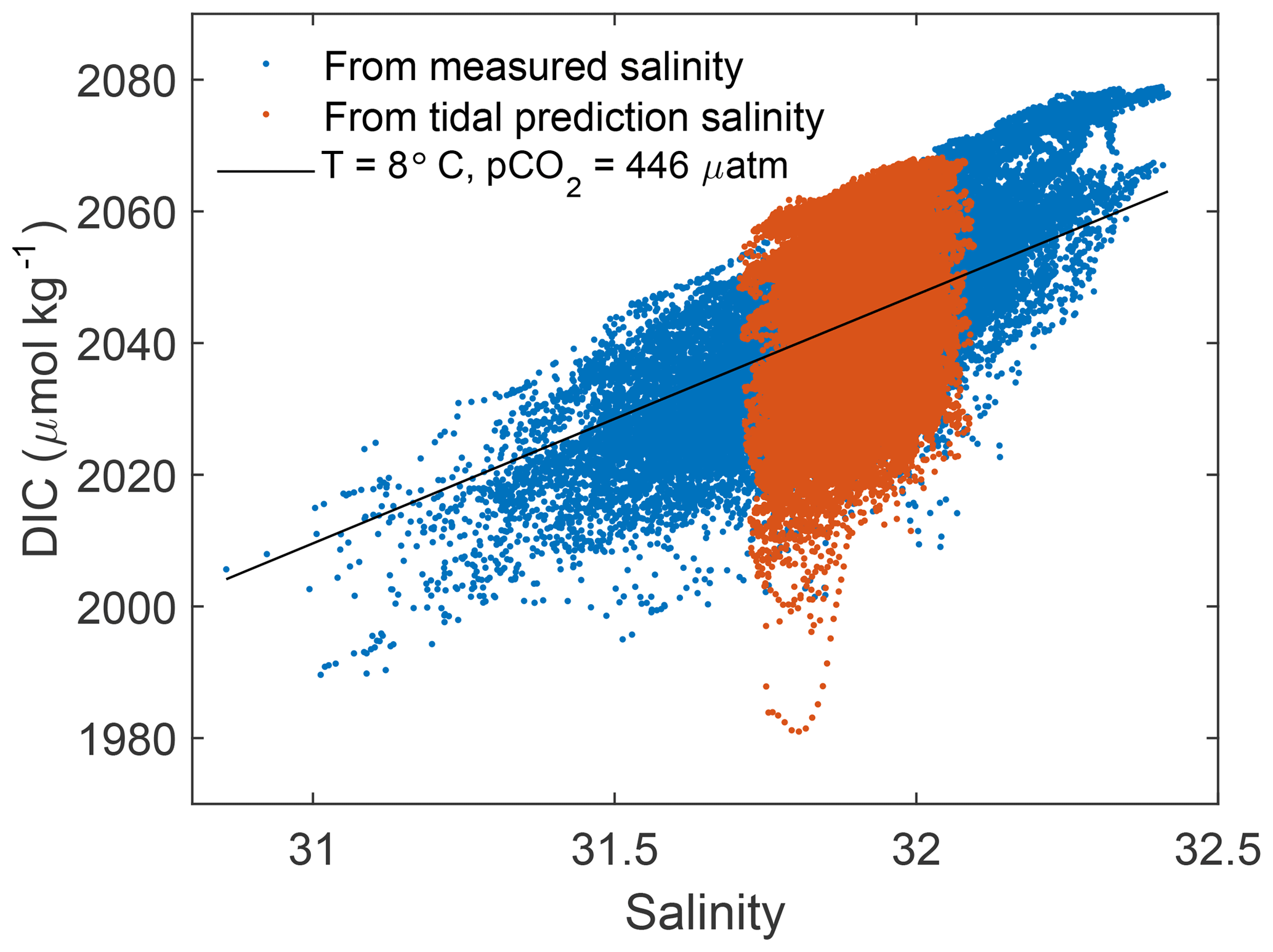
Figure 3DIC vs. salinity for measured (blue) and tidal reconstruction (orange) carbonate system solutions. DIC at fixed pCO2 (446 µatm) and temperature (8 ∘C) (black) is subtracted from observed DIC to create DICex.
Only the time variation of the resulting DICex is meaningful, not the absolute value. This time variation is not sensitive to the choice of fixed pCO2 and temperature from within the ranges typical of this field site. The relationship between pCO2 and DIC that is captured in DICex is unchanged over the small natural range of alkalinity in this region, so DICex is not sensitive to the choice of a measured, tidal harmonic, or even constant salinity estimate. DICex is presumed to be predominantly biogeochemically driven, but also includes any changes in DIC due to air–sea exchange, which we could not calculate on daily timescales, but are shown to be small on weekly timescales in Sect. 3.5.
DICex (Fig. 4a) decreases rapidly April and May due to the spring bloom and more gradually over the summer, as explained by Craig et al. (2015). Following a decline in October (yearday 270–290) suggestive of a fall bloom, DICex increases steadily through fall and winter. The daily cycle of DICex is evident throughout the year when highlighted by the use of color to indicate local time of day in Fig. 4a. Daily maxima occur in early morning (∼ 06:00, pink dots) following nighttime respiration and minima in late afternoon (∼ 17:00, green dots) following the peak hours of sunlight and photosynthesis. This cycle is shifted several hours earlier than the one reported on the Scotian Shelf by Thomas et al. (2012). The daily range of DICex is approximately 3 times as large in summer as in winter, consistent with higher summer sunlight supporting higher phytoplankton growth.
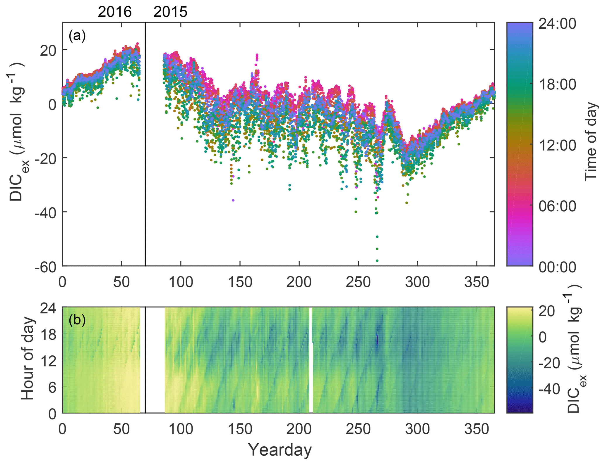
Figure 4(a) DICex for a calendar year with local time of day indicated by color. The time variation of the resulting DICex is meaningful, while the total value depends on the specific choice of fixed pCO2 used for the computation. (b) DICex (color) for each hour of the day over a calendar year.
The solar and tidal cycles combine to create a fortnightly cycle (visible in Fig. 4a, but more clear in Fig. 4b). This beating pattern in the time series is due to the difference between the 12.42 h M2 tidal and 24 h diel periods. Mathematically, this effect is identical to a spring–neap tidal variation, but here the daily cycle is due to solar insolation, rather than the solar gravitational force. The diagonal banding pattern in Fig. 4b shows the M2 tide progressing 50 min later each day. The daily morning peak and afternoon low appear as broad horizontal stripes and are most visible for yeardays 100–275. A similar daily pattern has been observed on the Scotian Shelf (Thomas et al., 2012), but no tidal signal was detected there. The pulsing of the strength of the morning high and afternoon low is due to the coincidence of an M2 maximum or minimum with the time of the daily maximum or minimum.
The overlapping daily and tidal cycles apparent in Fig. 4 can be separated and quantified by spectral analysis. Power spectral densities of DICex, for frequency f, were calculated by Welch's method on detrended time series for each month with eight approximately week-long Hamming windowed segments with 50 % overlap. The position of peaks in spectra of month-long DICex time series (Fig. 5a) identify the frequencies with the greatest variability, and the area under each peak equals the contribution of that frequency to the total signal variance. These February and August examples show a large daily peak and a slightly smaller M2 tidal peak for both months, and they show that DICex is more variable in August than February at all frequencies. The third and fourth peaks visible in Fig. 5a are harmonics of the 24 h and M2 frequencies and do not substantially contribute to the total signal variance. The variance of DICex at the 24 h and M2 frequencies are calculated from the area under the spectra using a five-point peak width, . The total DICex variance is 10 times higher in August than in February but in both seasons the daily and M2 frequencies represent the majority of the variability: 56 % (56 %) and 19 % (7 %), respectively, of the total DICex signal variance in August (February).
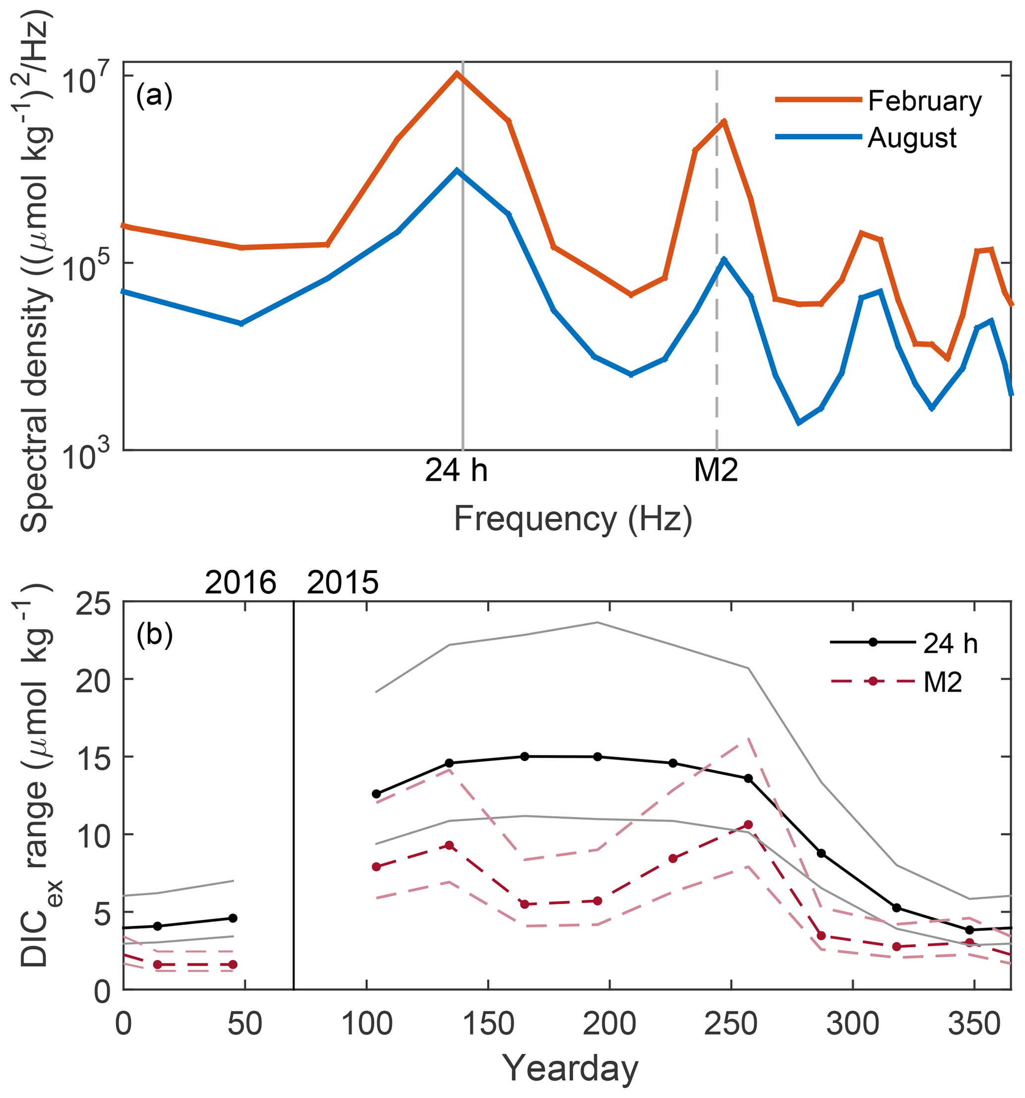
Figure 5(a) Spectra of DICex in February (blue) and August (orange). (b) DICex range over daily (black, solid) and M2 (red, dashed) cycles for each month of the year. Amplitude determined from area beneath peaks in spectra, such as examples shown in (a). The 95 % confidence intervals are shown in lighter colors.
The strengths of M2 and daily cycles in DICex evolve with the season (Fig. 5b). The range of DICex variation at a particular frequency is defined as 2A for amplitude A, i.e., the “peak-to-trough” difference of a sine wave. The rms value of a sinusoid equals , so the range of the daily or tidal DIC cycle equals . Months from April through September have a similar size daily signal near 15 µmol kg−1, with lower values throughout the winter. The tidal variation is always smaller than the daily variation but is also generally larger in summer and smaller in winter. However, unlike the daily signal, June and July have smaller tidal variation than the shoulder months of April, May, August, and September. Changes in the strength of the tidal signal reflect changes in spatial gradients of DICex, presumably owing to season fluctuations in the spatial variation of biological activity.
3.3 Tidal phasing
The relationships between the tidal flow and DICex, temperature, salinity and alkalinity, and are depicted in Fig. 6 for April 2015, when velocity measurements were available. This tidal-phase information complements the daily cycle of DICex emphasized in Fig. 4a.
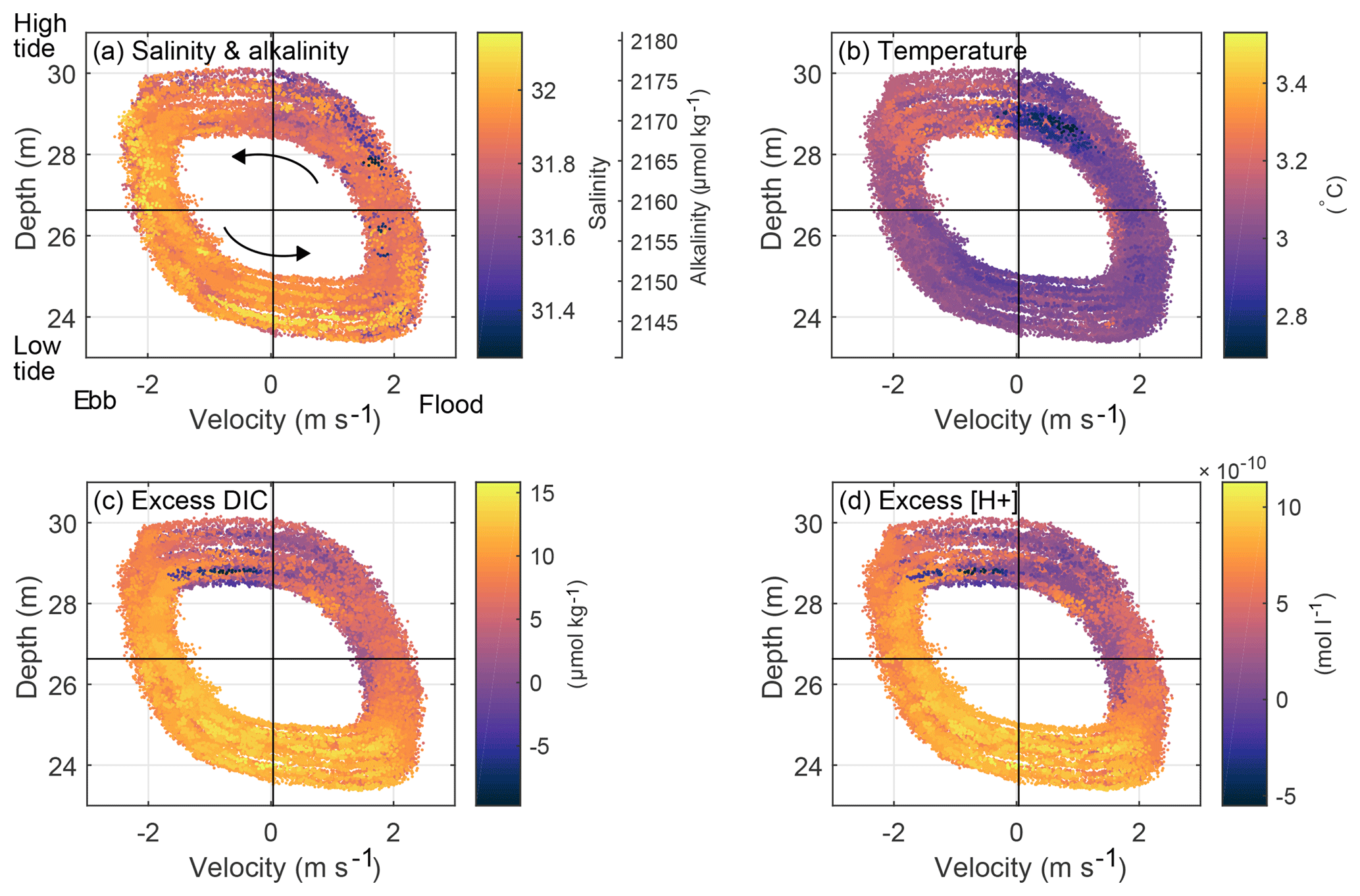
Figure 6The relationships between the tidal flow and (a) salinity and alkalinity, (b) temperature, (c) DICex, and (d) are depicted for April 2015, when velocity measurements were recorded. The phase of the tide is indicated by ADCP water depth on the y axis and depth-averaged along-channel velocity on the x axis (positive in flood direction, i.e., northward, into the Bay of Fundy), with mean values indicated by black lines. Phase progression is counterclockwise, shown by arrows in (a). Scalar concentration is indicated by color; for example, more yellow data points visible on the left side of (a) indicate higher salinity during ebb tide, when water is leaving the Bay of Fundy. The variation in position of the tidal ellipse between each pass of the tidal cycle reflects the changes in tidal range and maximum speed associated with the spring–neap cycle. For all variables shown by colors, 18 h high-pass-filtered values plus mean are plotted to visually highlight the M2 variability by eliminating the daily signal; the filtering is not used for data analyses. is computed using the same method as DICex, for .
Salinity and corresponding alkalinity (Fig. 6a) are lowest during late flood and highest between maximum ebb and early flood (see ebb and flood directions on Fig. 1). Salinity values are lower during flood compared to those on ebb, which indicates that the water from St. Mary's Bay/Scotian Shelf that enters the Bay of Fundy through Grand Passage each flood tide is fresher than what exits during ebb. This tidal asymmetry in salinity holds for all months of the year.
Temperature (Fig. 6b) is lowest in late flood and peaks a short time later during early ebb, and overall the water is colder during flood than during ebb. Unlike the salinity asymmetry, the temperature asymmetry changes sign with the seasons. The shallower St. Mary's Bay is more sensitive to surface heat fluxes than the deeper Bay of Fundy, so it is warmer in spring and summer and colder in fall and winter. As a result, the oscillating tides move heat into the Bay of Fundy half of the year and out half of the year.
DICex (Fig. 6c) peaks at low slack and the lowest values occur during late flood and early ebb. (Fig. 6d) also peaks at low slack and has the lowest values during early ebb. This pattern suggests lower net community production (NCP) in the bay than on the shelf, likely a result of a stronger spring bloom on the shelf than in the bay, which is advected by the mean currents around southern Nova Scotia. Smaller-scale spatial variation in nutrient or light availability owing to different water depths or mixing rates could also contribute to different growth rates on the two sides of Grand Passage.
3.4 Lateral transport by tidal pumping
Transport of carbon through Grand Passage is driven both by net volume transport and by tidal pumping – oscillatory tides moving water masses with different properties back and forth on each tidal cycle. Water volume flux per meter of channel width, q (m2 s−1) , for water depth h (m) and depth-averaged velocity (m s−1) can be decomposed into a time-mean (〈〉) and fluctuating (′) part, . By definition, there is no net water volume transport by the time-varying volume flux used to calculate tidal pumping. The fluctuations in volume transport (Fig. 7a) that drive tidal pumping vary in magnitude over the spring–neap cycle, but return to zero each tidal cycle.
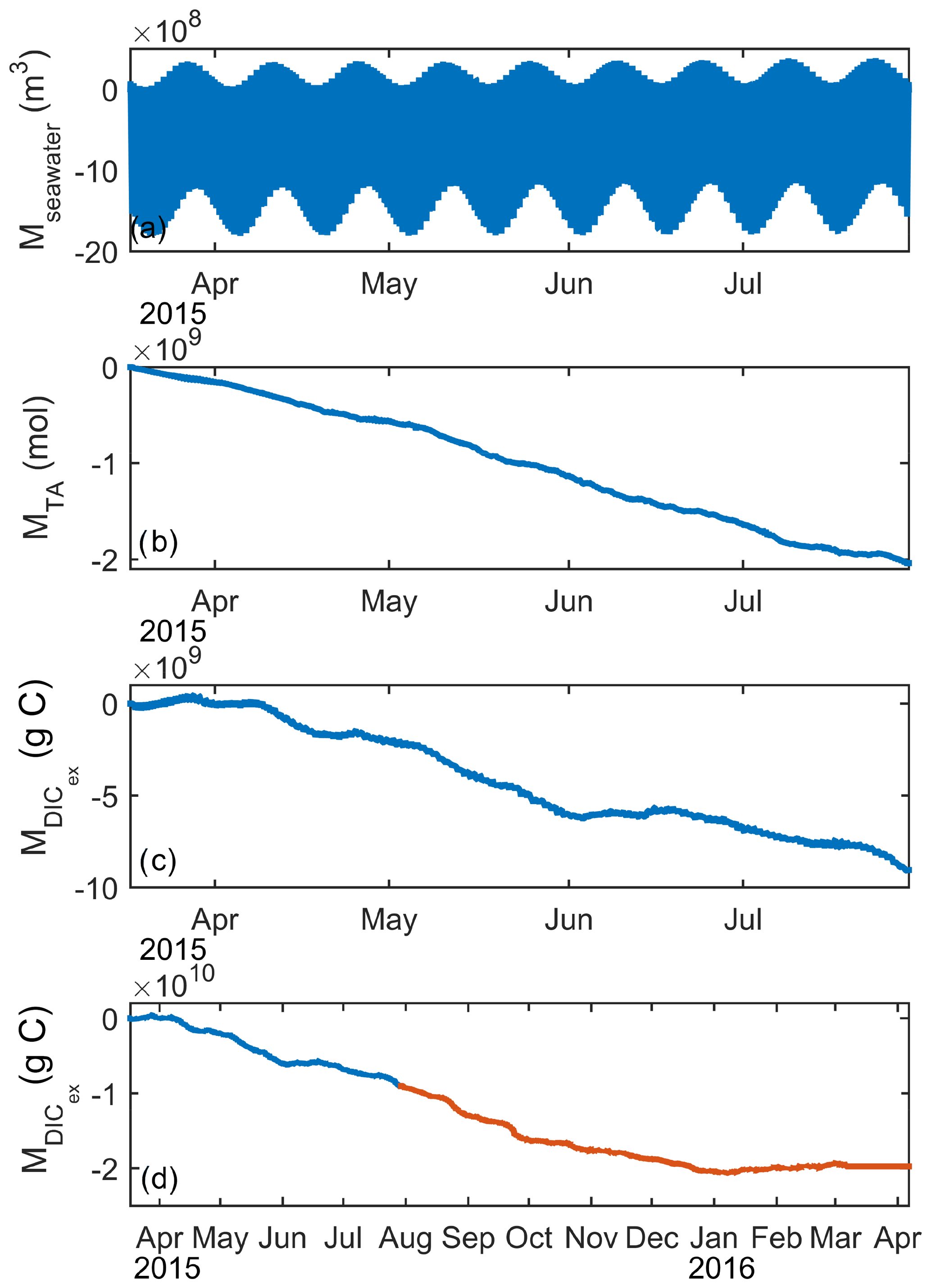
Figure 7Cumulative along-channel transport since the start of the deployment period by tidal pumping of (a) water volume, (b) alkalinity, and (c) DICex for March–July 2015 and (d) DICex for the full year; orange color indicates period not shown in (a)–(c). Salt or alkalinity fluxes are not computed for the full year because fluxes from the constructed tidal salinities will only reflect the mean trend already seen in Fig. 7b and not contain changes in phase or magnitude that might occur in the fall or winter.
Any correlation between the tidal water volume flux, q′, and fluctuations in conserved carbonate system concentration variables, (g m−3 or mol m−3), leads to a scalar flux by tidal pumping, ( or ), when averaged over timescales longer than a tidal cycle. Salinity is nearly vertically uniform at this field site (Razaz et al., 2019), and we assume DIC is also vertically uniform because the vertical mixing timescale is much shorter than the timescale of gas exchange owing to the high turbulence in the Bay of Fundy (Appendix A1), i.e., . Fluctuations of the conserved variable that are not correlated with fluctuations in water volume flux, such as the daily or seasonal cycles shown in Fig. 4a, are in S′ but do not contribute to because they are not correlated with q′.
Cumulative along-channel transports, M (m3, mol, or g C), of water volume, alkalinity, and DICex (Fig. 7) are calculated by multiplying q′, , and by the width (w=800 m) of Grand Passage and integrating in time, t. We assume spatial uniformity of water properties across the section.
The fluctuating water volume flux, q′, used to compute these transports is a tidal harmonic solution based on a fit to the month of ADCP data from April 2015. The harmonic fit represents 93 % of the observed variability (i.e., R=0.97) in water volume flux. By contrast, the tidal harmonic fit to the 4 months of salinity measurements (Sect. 2.1) is not well correlated with the observations (R=0.35), owing to the non-sinusoidal shape of the salinity signal as well as longer period variability. Due to this poor fit, alkalinity fluxes are not computed for the period without direct salinity measurements. DICex is not affected by the salinity, as described in Sect. 3.2, so DICex transport is calculated for the full year.
For the first half of 2015, salt and alkalinity (Fig. 7b) are pumped southward, out of the Bay of Fundy by the tides. DICex (Fig. 7c) also has net negative (southward) transport over this period, but has shorter periods of near-zero or positive transport in March, mid-April, and early June.
Tidal pumping for DICex is also calculated for the second half of the deployment year (Fig. 7d) and continues the negative trend until January 2016, when the flux becomes slightly positive for the last 2 months of the measurement period. Salinity from a seasonal climatology Richaud et al. (e.g 2016); Signorini et al. (e.g 2013) suggests that the sign of the lateral salinity gradient is the same all year, indicating that the sign of the alkalinity flux will stay the same throughout the year.
Notably, these transports move alkalinity and DICex in the opposite direction of the mean flow of the region, which follows the coast clockwise around southwestern Nova Scotia, moving northward into the Bay of Fundy near Grand Passage (e.g., Aretxabaleta et al., 2008). Within Grand Passage, salinity and alkalinity transport by tidal pumping is roughly 20 % of that by the mean volume flux through the channel (Appendix A2). The exact fraction may vary outside the channel, but the important point is that tidal pumping likely plays a first-order role in carbon transport budgets anywhere with large tides and spatial gradients in the biogeochemical water properties, including the entire width of the mouth of the Bay of Fundy.
While the mean volume transport through Grand Passage cannot be extrapolated to the full width of the Bay of Fundy, the tidal pumping term could plausibly apply over the eastern side of the mouth, where salinity gradients are positive into the bay. If the transport by tidal pumping is applied out to just 10 km from shore (∼15 % of the width of the mouth of the bay), which is a ∼50 m deep region, the DICex transported out of the Bay of Fundy through lateral advection by tidal pumping would be 5×10⁸ kg C in a year. This value is 3 times what is estimated to leave the Bay of Fundy by outgassing to the atmosphere if the Grand Passage air–sea fluxes (Sect. 3.5) applied over the whole bay.
3.5 Air–sea CO2 flux
High-frequency variability in DICex is assumed to be driven by biological and biogeochemical processes, but air–sea flux plays a significant role on long timescales. We assess the importance of air–sea flux to the carbon budget by calculating weekly and annual fluxes, as well as the equivalent changes in DIC. Oceanic pCO2 was lower than atmospheric pCO2 (Fig. 2a) for the first 2 months of observations, April and May, and then rose and remained higher than atmospheric pCO2 for the following 10 months, June through March, giving an annual net negative CO2 flux (i.e., outgassing) at this site.
Atmospheric and oceanic CO2 concentrations (Fig. 2a) and wind speed (Sect. 2.3) are used to calculate the flux of CO2 between the atmosphere and ocean at the field site. Atmospheric and oceanic pCO2 data were interpolated onto the hourly wind time base. Air–sea flux, F (), is calculated following Wanninkhof et al. (2009) Eq. (3), here using the convention that F is positive for a flux of gas from the atmosphere into the ocean.
where K0 is the solubility of CO2 () and k (m s−1) is gas transfer velocity. k (cm h−1) can be represented well for wind speeds, U (m s−1), below 15 m s−1 at Schmidt number Sc=660 with the empirical formula (Wanninkhof et al., 2009, Eq. 37)
U10 is the 10 m wind speed measured at the ECCC station on Brier Island. U10 was also computed as the difference between the air and water speeds (up to ±2 m s−1), which increased the air–sea flux estimates by approximately 5 %. Air–sea flux is initially computed on an hourly timescale to fully capture the quadratic wind-speed dependence, but only weekly (or longer) averages of F are robust owing to the weekly timescale of the available atmospheric pCO2 data.
The average air–sea CO2 flux at this site is , which is similar in magnitude to previous Gulf of Maine flux estimates, but with outgassing most of the year rather than the more even split between positive and negative fluxes reported at a deeper site (Vandemark et al., 2011) or for regional averages (Signorini et al., 2013; Cahill et al., 2016). If this gas exchange was spatially uniform over the Bay of Fundy (approx. 104 km2), this air–sea flux would release 1.75×10⁸ kg carbon ( mol) into the atmosphere per year.
The annual local flux is equivalent to a −47 µmol kg−1 change in DICex (Eq. 6) when applied to 30 m water depth in Grand Passage over the year-long deployment.
The weekly averaged flux is typically between 0 and , which is equivalent to up to −2 µmol kg−1 change in DICex over a week. The maximum weekly value occurred in late September 2015 and was , yielding a −4 µmol kg−1 change in DICex in 1 week.
3.6 Consideration of the local DIC budget
Observed DICex variation is due to the difference between local (water column and sediment) net community production, local air–sea flux, and advective changes due to spatial gradients of biological production or air–sea flux (Appendix A3). Daily variation in DICex can reasonably be attributed to the local time rate of change, and the tidal variation is likely advective. Longer cycles of variation could have both a local seasonal cycle and advective contributions from seasonal variation occurring weeks or months upstream.
We did not directly measure spatial gradients of DICex, but can infer that the local along-channel gradient is positive (increasing northwards) from the observation that the highest and lowest values tend to occur near low and high slack water, respectively (Fig. 6). A positive along-channel DICex gradient carried by a northward regional circulation decreases local DICex.
DICex returns near to its initial value over the full annual cycle (Fig. 4a) so the annual mean is zero. The outgassing air–sea flux and along-channel advection both decrease DICex, so to close the DIC budget (Eq. A6) the biologically driven change in DIC must be positive (NCP<0) on average over the year, even though it is negative in the spring.
Open ocean carbon cycles can be described by annual and daily variations and taken to be uniform over large spatial scales. However, near the coast, ecosystems change markedly over short distances, so the dynamics of the carbonate system cannot be well described without resolving the spatial variation or capturing the effects of lateral advection.
In this work, we unravel tidal advection from the diel production and respiration cycles due to solar radiation and show that the tides pump both alkalinity and DIC out of the Bay of Fundy into the open ocean, opposite to the transport via the residual flow. This tidal pumping process, in contrast to any residual flow, does not result in a net transport of water, but can greatly enhance the exchange of passive scalars like DIC. In regions with strong tidal currents and spatial variation in biological activities, tidal pumping could substantially modulate the coastal ocean's response to global ocean acidification.
High-frequency measurements reveal previously unaccounted for tidal variations in the carbonate system, in addition to more precise quantification of the familiar daily cycles and annual blooms. These results are crucial prerequisites to a deeper understanding of coastal systems' resilience or vulnerability to anthropogenic change.
The data that support the findings of this study are available from the corresponding author upon reasonable request.
A1 Vertical mixing
In this highly turbulent, unstratified water column, the vertical mixing timescale (Eq. A1) is much shorter than the timescale of gas exchange (Eq. A2).
where h is total water depth at the ADCP site; the k660 value is the average from the data set; Aν is eddy viscosity estimated as the mid-water-depth value of a cubic eddy viscosity profile for a logarithmic near-bed velocity profile and zero surface wind stress (e.g., Lentz, 1995); κ is the von Kármán constant; and u* is the shear velocity with the value chosen from the Grand Passage site GP2 from McMillan et al. (2013), which is very close to the site of the present study.
A2 Mean volume transport
The mean volume flux, 〈q〉, is derived from both the mean depth-averaged along-channel velocity and the mean volume transport due to asymmetries in the tidal cycle . At the ADCP location, m s−1 and 〈h〉=26.6 m, which are indicated by the solid black lines in Fig. 6, yielding 0.95 m2 s−1 volume flux.
The position of the data points in Fig. 6 compared to the mean axes made by and 〈h〉 values shows that the water tends to be deeper during ebb than during flood. If the tide was a perfect standing wave (slack at high and low water, and maximum ebb and flood speeds occurring at the mean water depth), the shape of the depth-velocity points would form a circle. The mean volume flux due to this tidal asymmetry, m2 s−1, which is larger than, and in the opposite direction of, the volume flux by the mean depth-averaged velocity.
Assuming spatial uniformity over the channel width, the volume flux driven by the mean depth-averaged velocity applied to the mean salinity of 31.9 yields a salt flux of 2.3×10⁴ kg s−1, and the volume flux driven by tidal asymmetry generates a salt flux of kg s−1.
The salt flux driven by total 〈q〉 from both components is kg s−1, which is 5 times the salt flux by tidal pumping shown in Fig. 7. However, the mean velocity and especially the phase lag between the tide depth and velocity is generated by friction and therefore sensitive to the specific channel geometry (e.g., Geyer and MacCready, 2014) and may vary across the mouth of the Bay of Fundy.
A3 Budget for biological DIC production
The change in observed DICex is given by
Biology and air–sea exchange both drive local changes in time, and both could potentially have changes in time due to advection of spatial gradients, which is what we (almost definitely) observe over the tidal cycle. For example,
where x is the along-channel distance and corresponds to local carbon consumption (i.e., equal to −NCP). So in total
If we assume the air–sea flux is spatially uniform, , then the change in observed DIC that is attributable to biological activity, DICbio, is given by
RMH performed the research and wrote the manuscript with the guidance of HT, who, with AEH, initially conceived of the project. RMH and HT developed the analysis trajectory. AEH provided velocity, temperature, salinity, and pressure data. RC and WB programmed, deployed, and maintained the instruments. JS provided Gulf of Maine salinity and alkalinity data. All authors consulted on the manuscript.
The authors declare that they have no conflict of interest.
This work was funded by the MEOPAR Canadian Ocean Acidification
Research Program (COARp) and the
Environment and Climate Change Canada (ECCC) Gulf of Maine Initiative. Thanks
to Walter Judge for instrument preparation and deployment, to Brittany Curtis
and Jonathan Lemay for water sample collection, and Mike Huntley and his crew
on the Nova Endeavor. We thank our anonymous reviewers for their
thoughtful and constructive feedback.
Edited by: Minhan Dai
Reviewed by: two anonymous referees
Aretxabaleta, A. L., McGillicuddy, D. J., Smith, K. W., and Lynch, D. R.: Model simulations of the Bay of Fundy Gyre: 1. Climatological results, J. Geophys. Res.-Oceans, 113, C10027, https://doi.org/10.1029/2007JC004480, 2008. a, b, c
Bigelow, H. B.: Physical oceanography of the Gulf of Maine, Bulletin of the U.S. Bureau of Fisheries, 40, 511–1027, 1927. a
Cahill, B., Wilkin, J., Fennel, K., Vandemark, D., and Friedrichs, M. A. M.: Interannual and seasonal variabilities in air-sea CO2 fluxes along the U.S. eastern continental shelf and their sensitivity to increasing air temperatures and variable winds, J. Geophys. Res.-Biogeo., 121, 295–311, https://doi.org/10.1002/2015JG002939, 2016. a, b
Codiga, D. L.: Unified Tidal Analysis and Prediction Using the UTide Matlab Functions, Technical Report 2011-01, 59 pp., Graduate School of Oceanography, University of Rhode Island, Narragansett, RI, available at: http://www.po.gso.uri.edu/~codiga/utide/utide.htm (last access: 14 January 2019), 2011. a
Craig, S. E., Thomas, H., Jones, C. T., Li, W. K., Greenan, B. J., Shadwick, E. H., and Burt, W. J.: The effect of seasonality in phytoplankton community composition on CO2 uptake on the Scotian Shelf, J. Marine Syst., 147, 52–60, https://doi.org/10.1016/j.jmarsys.2014.07.006, 2015. a, b
Dever, M., Hebert, D., Greenan, B., Sheng, J., and Smith, P.: Hydrography and Coastal Circulation along the Halifax Line and the Connections with the Gulf of St. Lawrence, Atmos. Ocean, 54, 199–217, https://doi.org/10.1080/07055900.2016.1189397, 2016. a, b
Dickson, A. and Millero, F.: A comparison of the equilibrium constants for the dissociation of carbonic acid in seawater media, Deep-Sea Res. Pt. A, 34, 1733–1743, https://doi.org/10.1016/0198-0149(87)90021-5, 1987. a
Dickson, A. G., Sabine, C. L., and Christian, J. R. (Eds.): Guide to best practices for ocean CO2 measurements, PICES Special Publication 3, 191 pp., North Pacific Marine Science Organization, Sidney, British Columbia, Canada, 2007. a
Dlugokency, E., Masarie, K., Lang, P., and Tans, P.: NOAA Greenhouse Gas Reference from Atmospheric Carbon Dioxide Dry Air Mole Fractions from the NOAA ESRL Carbon Cycle Cooperative Global Air Sampling Network, available at: http://www.esrl.noaa.gov/gmd/ccgg/mbl/data.php (last access: 14 January 2019), data Path: ftp://aftp.cmdl.noaa.gov/data/trace_gases/co2/flask/surface/ (last access: 14 January 2019), 2015. a
Fisheries and Oceans Canada: Atlantic Zone Monitoring Program (AZMP), available at: http://www.meds-sdmm.dfo-mpo.gc.ca/isdm-gdsi/azmp-pmza/index-eng.html (last access: 14 January 2019), 2013–2014. a
Garrett, C.: Tidal Resonance in the Bay of Fundy and Gulf of Maine, Nature, 238, 441–443, https://doi.org/10.1038/238441a0, 1972. a
Geyer, W. R. and MacCready, P.: The Estuarine Circulation, Annu. Rev. Fluid Mech., 46, 175–197, https://doi.org/10.1146/annurev-fluid-010313-141302, 2014. a
Gledhill, D. K., White, M. M., Salisbury, J., Thomas, H., Mlsna, I., Liebman, M., Mook, B., Grear, J., Candelmo, A. C., Chambers, R. C., Gobler, C. J., Hunt, C. W., King, A. L., Price, N. N., Signorini, S. R., Stancioff, E., Stymiest, C., Wahle, R. A., Waller, J. D., Rebuck, N. D., Wang, Z. A., Capson, T. L., Morrison, J. R., Cooley, S. R., and Doney, S. C.: Ocean and Coastal Acidification off New England and Nova Scotia, Oceanography, 28, 182–197, https://doi.org/10.5670/oceanog.2015.41, 2015. a
Greenberg, D. A.: Modelling the Mean Barotropic Circulation in the Bay of Fundy and Gulf of Maine, J. Phys. Oceanogr., 13, 886–904, https://doi.org/10.1175/1520-0485(1983)013<0886:MTMBCI>2.0.CO;2, 1983. a, b
Hannah, C. G., Shore, J. A., Loder, J. W., and Naimie, C. E.: Seasonal Circulation on the Western and Central Scotian Shelf, J. Phys. Oceanogr., 31, 591–615, https://doi.org/10.1175/1520-0485(2001)031<0591:SCOTWA>2.0.CO;2, 2001. a, b
Houghton, R. and Fairbanks, R.: Water sources for Georges Bank, Deep-Sea Res. Pt. II, 48, 95–114, https://doi.org/10.1016/S0967-0645(00)00082-5, 2001. a
Lentz, S. J.: Sensitivity of the Inner-Shelf Circulation to the Form of the Eddy Viscosity Profile, J. Phys. Oceanogr., 25, 19–28, https://doi.org/10.1175/1520-0485(1995)025<0019:SOTISC>2.0.CO;2, 1995. a
Lewis, E. and Wallace, D. W. R.: Program Developed for CO2 System Calculations, ORNL/CDIAC-105, Tech. rep., Carbon Dioxide Information Analysis Center, Oak Ridge National Laboratory, U.S. Department of Energy, Oak Ridge, Tennessee, 1998. a
Magenheimer, J. F., Moore, T. R., Chmura, G. L., and Daoust, R. J.: Methane and carbon dioxide flux from a macrotidal salt marsh, Bay of Fundy, New Brunswick, Estuaries, 19, 139–145, https://doi.org/10.2307/1352658, 1996. a
McMillan, J. M., Schillinger, D. J., and Hay, A. E.: Southwest Nova Scotia Resource Assessment, Volume 3: Acoustic Doppler Current Profiler Results, Tech. rep., Offshore Energy Research Association, available at: http://www.oera.ca/wp-content/uploads/2013/07/SWNT_Final-Report_Volume-3.pdf (last access: 14 January 2019), 2013. a
Nidzieko, N. J., Needoba, J. A., Monismith, S. G., and Johnson, K. S.: Fortnightly Tidal Modulations Affect Net Community Production in a Mesotidal Estuary, Estuar. Coast., 37, 91–110, https://doi.org/10.1007/s12237-013-9765-2, 2014. a
Pawlowicz, R., Beardsley, B., and Lentz, S.: Classical Tidal Harmonic Analysis Including Error Estimates in MATLAB using T_TIDE, Comput. Geosci., 28, 929–937, 2002. a
Pettigrew, N. R., Churchill, J. H., Janzen, C. D., Mangum, L. J., Signell, R. P., Thomas, A. C., Townsend, D. W., Wallinga, J. P., and Xue, H.: The kinematic and hydrographic structure of the Gulf of Maine Coastal Current, Deep-Sea Res. Pt. II, 52, 2369–2391, https://doi.org/10.1016/j.dsr2.2005.06.033, 2005. a
Razaz, M., Zedel, L., Hay, A. E., and Kawanisi, K.: Monitoring Tidal Currents in a Well-Mixed, Narrow Strait Using High-Frequency Acoustic Tomography, J. Geophy. Res., in review, 2019. a
Richaud, B., Kwon, Y.-O., Joyce, T. M., Fratantoni, P. S., and Lentz, S. J.: Surface and bottom temperature and salinity climatology along the continental shelf off the Canadian and U.S. East Coasts., Cont. Shelf Res., 124, 165–181, https://doi.org/10.1016/j.csr.2016.06.005, 2016. a
Salisbury, J., Vandemark, D., Hunt, C., Campbell, J., Jonsson, B., Mahadevan, A., McGillis, W., and Xue, H.: Episodic riverine influence on surface {DIC} in the coastal Gulf of Maine, Estuar. Coast. Shelf S., 82, 108–118, https://doi.org/10.1016/j.ecss.2008.12.021, 2009. a
Salisbury, J. E.: Dissolved inorganic carbon, total alkalinity, pH, nutrients and other variables collected from profile and discrete sample observations using CTD, Niskin bottle, and other instruments from NOAA Ship Gordon Gunter off the U.S. East Coast during the East Coast Ocean Acidification (GU-15-04 ECOA1) from 2015-06-20 to 2015-07-23 (NCEI Accession 0159428), Version 2.2, NOAA National Centers for Environmental Information, Dataset, https://doi.org/10.7289/V5VT1Q40, 2017. a
Shadwick, E. H. and Thomas, H.: Seasonal and spatial variability in the CO2 system on the Scotian Shelf (Northwest Atlantic), Mar. Chem., 160, 42–55, https://doi.org/10.1016/j.marchem.2014.01.009, 2014. a
Shadwick, E. H., Thomas, H., Comeau, A., Craig, S. E., Hunt, C. W., and Salisbury, J. E.: Air-Sea CO2 fluxes on the Scotian Shelf: seasonal to multi-annual variability, Biogeosciences, 7, 3851–3867, https://doi.org/10.5194/bg-7-3851-2010, 2010. a
Shadwick, E. H., Thomas, H., Azetsu-Scott, K., Greenan, B., Head, E., and Horne, E.: Seasonal variability of dissolved inorganic carbon and surface water pCO2 in the Scotian Shelf region of the Northwestern Atlantic, Mar. Chem., 124, 23–37, https://doi.org/10.1016/j.marchem.2010.11.004, 2011. a
Signorini, S. R., Mannino, A., Najjar, R. G., Friedrichs, M. A. M., Cai, W.-J., Salisbury, J., Wang, Z. A., Thomas, H., and Shadwick, E.: Surface ocean pCO2 seasonality and sea-air CO2 flux estimates for the North American east coast, J. Geophys. Res.-Oceans, 118, 5439–5460, https://doi.org/10.1002/jgrc.20369, 2013. a, b, c
Smith, P. C.: Seasonal and Interannual Variability of Current, Temperature and Salinity off Southwest Nova Scotia, Can. J. Fish. Aquat. Sci., 46, s4–s20, https://doi.org/10.1139/f89-275, 1989. a
Smith, P. C., Houghton, R. W., Fairbanks, R. G., and Mountain, D. G.: Interannual variability of boundary fluxes and water mass properties in the Gulf of Maine and on Georges Bank: 1993–1997, Deep-Sea Res. Pt. II, 48, 37–70, https://doi.org/10.1016/S0967-0645(00)00081-3, 2001. a
Thomas, H., Craig, S. E., Greenan, B. J. W., Burt, W., Herndl, G. J., Higginson, S., Salt, L., Shadwick, E. H., and Urrego-Blanco, J.: Direct observations of diel biological CO2 fixation on the Scotian Shelf, northwestern Atlantic Ocean, Biogeosciences, 9, 2301–2309, https://doi.org/10.5194/bg-9-2301-2012, 2012. a, b, c
van Heuven, S., Pierrot, D., Rae, J. W. B., Lewis, E., and Wallace, D. W. R.: MATLAB Program Developed for CO2 System Calculations, ORNL/CDIAC-105b, Carbon Dioxide Information Analysis Center, Oak Ridge National Laboratory, U.S. Department of Energy, Oak Ridge, Tennessee, https://doi.org/10.3334/CDIAC/otg.CO2SYS_MATLAB_v1.1, 2011. a
Vandemark, D., Salisbury, J. E., Hunt, C. W., Shellito, S. M., Irish, J. D., McGillis, W. R., Sabine, C. L., and Maenner, S. M.: Temporal and spatial dynamics of CO2 air-sea flux in the Gulf of Maine, J. Geophys. Res.-Oceans, 116, c01012, https://doi.org/10.1029/2010JC006408, 2011. a, b
Wang, Z. A., Kroeger, K. D., Ganju, N. K., Gonneea, M. E., and Chu, S. N.: Intertidal salt marshes as an important source of inorganic carbon to the coastal ocean, Limnol. Oceanogr., 61, 1916–1931, https://doi.org/10.1002/lno.10347, 2016. a
Wanninkhof, R., Asher, W. E., Ho, D. T., Sweeney, C., and McGillis, W. R.: Advances in Quantifying Air-Sea Gas Exchange and Environmental Forcing, Annu. Rev. Mar. Sci., 1, 213–244, https://doi.org/10.1146/annurev.marine.010908.163742, 2009. a, b
Weiss, R.: Carbon dioxide in water and seawater: the solubility of a non-ideal gas, Mar. Chem., 2, 203–215, https://doi.org/10.1016/0304-4203(74)90015-2, 1974. a