2.1 Site description

The study sites in the Kraichgau region (KR) were located at “Katharinentalerhof”, characterized by mostly flat terrain, and are located approximately 4 km north of the city Pforzheim (48.92^∘ N, 8.70^∘ E). Three EC stations (EC1, EC2, and EC3) were installed at adjacent fields with the respective areas of 14.9, 23.6, and 15.8 ha (Fig. 1). The prevailing wind direction is west. A former landfill site is located approximately 500 m to the south of the experimental fields whose maximum elevation is about 41 m above its surroundings. KR is one of the warmest regions in Germany, with a mean temperature and annual precipitation of 9.4 ^∘C and 890 mm in 1981–2010 (meteorological station Pforzheim-Ispringen, German Weather Service, located about 3 km from the research sites). The soils of this region developed from deep loess layers overlying a shell limestone. Detailed information about meteorological and soil conditions can be found in Table 1 and in Imukova et al. (2016), Ingwersen et al. (2015), and Wizemann et al. (2014).

Table 1Main characteristics of the investigated sites.

Download Print Version | Download XLSX

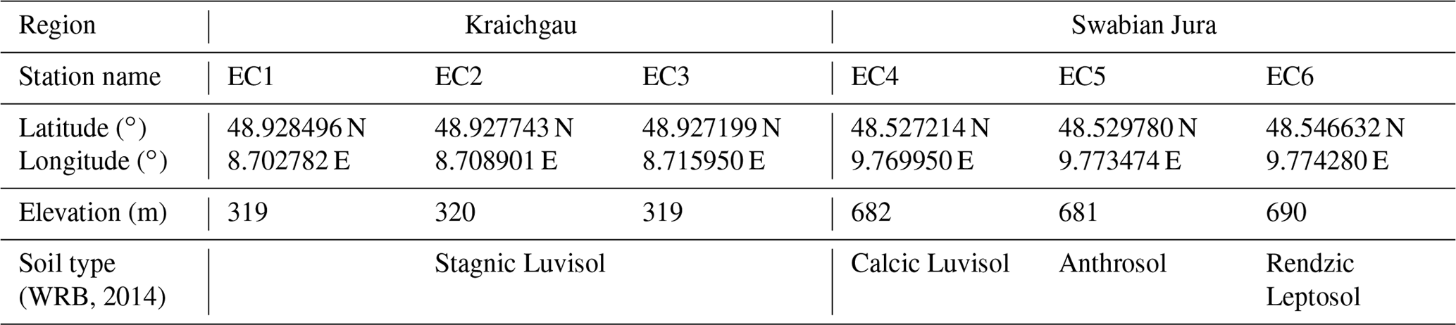
Due to its higher elevation, the Swabian Jura region (SJ) is characterized by a colder and harsher climate compared to KR. The prevailing wind direction is southwest to west. Mean temperature and annual precipitation were 7.5 ^∘C and 1042 mm in 1981–2010 (Meteorological station Merklingen, German Weather Service, about 2 km from the research sites). Information about meteorological and soil variables is given in Table 1. Accordingly, crops are generally sowed and harvested later than in KR. SJ is the largest contiguous karst landscape in Germany, with generally rather shallow soils. The study sites are located close to the town of Merklingen (Fig. 1). The areas of the three research fields at EC4, EC5, and EC6 were 8.7, 16.7, and 13.4 ha, respectively. While EC4 and EC5 were adjacent fields, EC6 was situated 1.5 km to the north (Fig. 1).

Table 2Crop grown at the six study sites from 2010 to 2017 (harvest year).

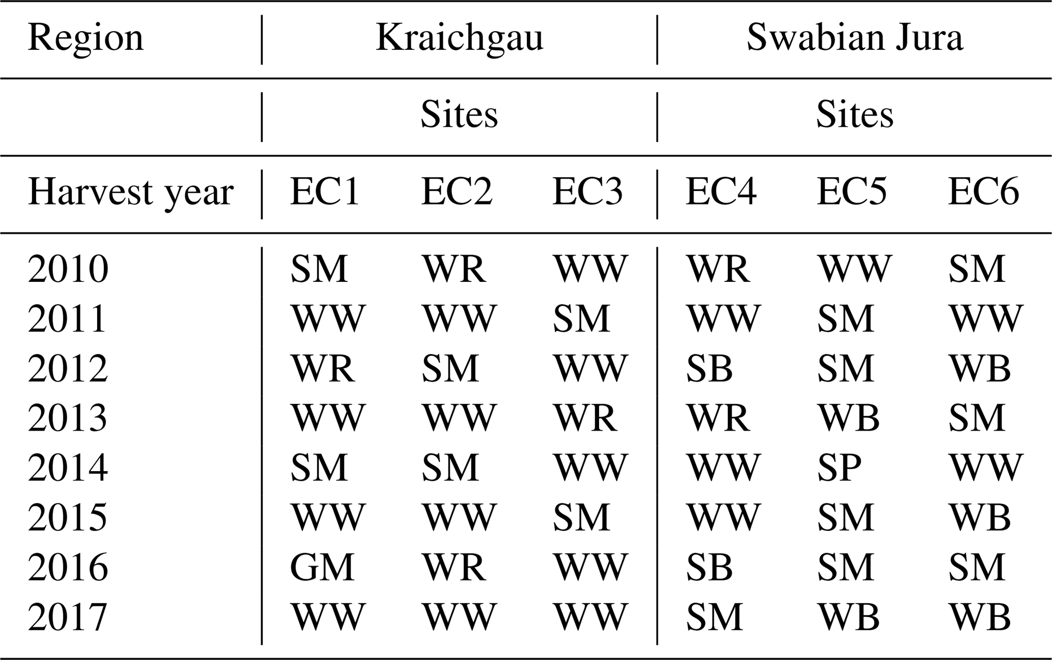
WW is winter wheat, WR is winter rapeseed, SM is silage maize, GM is grain maize, SB is summer barley, WB is winter barley, and SP is spelt.

Download Print Version | Download XLSX

The crop rotation in SJ was more diverse than in KR, and the most frequently grown crops were winter wheat and silage maize (Table 2). In 50 % of the years on-site in KR, winter wheat was cultivated; this value was only 25 % in SJ. KR showed a lower variety in cultivated crops to SJ, with three in KR and six in SJ. At all sites, farmers frequently grew cover crops between winter and summer crops. These were mainly mustard, phacelia, or multi-species mixtures.

2.2 Eddy-covariance measurements

One EC station was installed at the center of each field site in spring 2009 (Ingwersen et al., 2011; Wizemann et al., 2014). All stations were equipped with a fast-response CO₂∕H₂O open-path infrared gas analyzer (LI-7500; LI-COR Biosciences, Lincoln, NE, USA) and a three-axis ultrasonic anemometer (CSAT3; Campbell Scientific Inc., Logan, UT, USA). The raw data of the gas analyzer and sonic anemometer were recorded at 10 Hz and stored on a CR3000 data logger (Campbell Scientific Inc., Logan, UT, USA). In early 2009, the CSAT3 orientation at EC1 and EC3 was 230^∘, and at EC2, it was 255^∘. In late April 2010, the orientation was changed to 170^∘ and varied over the subsequent years between 160 and 190^∘, ensuring that winds from the prevailing wind direction (west and east) enter the anemometer from the side. In SJ, the mean CSAT3 orientation was $\mathrm{220}{}^{\circ }\pm \mathrm{15}$ from late March 2010 until the end of 2017. The gas analyzers were factory-calibrated biannually. Sensor heights were adjusted to account for increasing canopy heights, particularly during the vegetation periods of maize. This ensured that the distance between sensors and canopy was roughly 2–3 m. Maximal sensor heights in KR and SJ were 6.00 m at EC2 (2014) and 4.80 m at EC6 (2010), and the minimal sensor height was approximately 2 m in both regions. Each EC system was powered by two 12 V batteries (each 240 Ah) charged by four 20 W solar panels. To enable continuous EC measurements during winter, portable fuel cell systems (Efoy Pro 800 Duo, FSC Energy AG, Brunnthal-Nord, Germany) were installed in autumn 2015: one at EC2 and one at EC6. At the others stations the LI-7500 was shut down during the winter, mostly from late November to mid-March.

Net radiation was measured using a four-component radiometer (NR01, Hukseflux Thermal Sensors, Delft, The Netherlands). The radiometers were placed above the cropped field area in close proximity to the EC stations. Air temperature and relative humidity were measured at a height of 2 m at each EC station using a temperature and relative humidity probe (HMP45C, Vaisala Inc, Helsinki, Finland). Soil temperature was measured at the depths of 0.02, 0.06, 0.15, 0.30, and 0.45 m (107 Thermistor probe, Campbell Scientific Inc., Logan, UT, UK). To measure the soil heat flux near the EC stations, three heat flux plates (HFP01, Hukseflux Thermal sensors, Delft, The Netherlands) were installed at a depth of 0.08 m. The soil volumetric water content at 0.05, 0.15, 0.30, 0.45, and 0.75 m depth was monitored with frequency-domain reflectometry sensors (CS616, Campbell Scientific Inc., Logan, UT, USA). In the shallow soil at EC6, however, soil variables could be measured only down to 0.3 m. Data from thermistor (0.02 and 0.06 m) and water content sensors (0.05 m) were used to calculate the soil heat storage between the soil heat flux plates and the ground surface (Eshonkulov et al., 2019; Wizemann et al., 2014). Precipitation was measured with a 0.2 mm tipping bucket rain gauge (ARG 100, Environmental Measurements Ltd., North Shields, UK), which was installed 1 m above ground. The rain gauges were recalibrated once per year.

2.3 Energy balance closure of eddy-covariance measurements

In the ideal case, the surface energy balance obeys the following equation:

where R_n is the incoming net radiation, LE is the latent heat flux, H is the sensible heat flux (both positive upwards), and G is the ground heat flux (positive downwards). All components are expressed in W m⁻². Note that in Eq. (1) minor flux terms such as energy storage in the canopy or energy conversion by photosynthesis are neglected. All available filtered half-hourly flux data of the four terms in Eq. (1) were used to calculate the EBC. Three measures were used to evaluate the EBC. Firstly, we determined the slope and intercept from ordinary linear regression (OLR) of turbulent fluxes (H+LE) against available energy (R_n−G). In the ideal case of a fully closed energy balance, the slope and intercept of the linear regression are equal to 1 and zero, respectively (Ping et al., 2011; Wilson et al., 2002). In this study, we also considered the intercept (W m⁻²) of the OLR in evaluating EBC, as suggested by Franssen et al. (2010).

Secondly, we calculated the energy balance ratio (EBR) as

Thirdly, we compared the energy balance residual (Res; W m⁻²) given by

2.4 Atmospheric conditions

As a proxy for the role of shear and buoyancy in the production or consumption of turbulent kinetic energy, we used the friction velocity, u^∗ (m s⁻¹), and the kinematic virtual temperature flux, respectively. The latter is the covariance ($w^{\prime }{T}_{\mathrm{v}}^{\prime })$ between vertical wind speed (w) and virtual temperature (T_v). As the virtual temperature can be replaced by the sonic temperature (T_s) with negligible loss of accuracy (Kaimal and Gaynor, 1991), we computed the virtual temperature flux from the covariance ($w^{\prime }{T}_{\mathrm{s}}^{\prime })$ between w and T_s.

The relationship between atmospheric stability and the EBC was examined using the dimensionless atmospheric stability parameter ζ defined by Stull (1988):

where z_m (m) is the measurement height of the sonic anemometer and L (m) is the Obukhov length. The stability parameter expresses the relative roles of shear and buoyancy. Using ζ, the stability of the atmosphere can be divided into three classes (Franssen et al., 2010): stable (ζ≥0.1), neutral (−0.1<ζ<0.1), and unstable ($\mathit{\zeta }\le -\mathrm{0.1}$).

2.5 Footprint analyses and micro-topography

To determine the relationship between the contributing source area of turbulent fluxes and the EBC, we performed footprint analyses. We used the flux footprint prediction online tool of a simple two-dimensional parameterization (Kljun et al., 2015, http://geography.swansea.ac.uk/nkljun/ffp/www/, last access: 17 July 2018). The footprint parameterization uses the Lagrangian stochastic particle dispersion model (Kljun et al., 2002). As input parameters to the model, we used displacement height, z_d (m), mean wind speed (m s⁻¹), Obukhov length (m), standard deviation of horizontal wind speed (m s⁻¹), friction velocity, u^∗ (m s⁻¹), wind direction (^∘), and measurement height above the ground surface, z_m (m), which was calculated by

where z_receptor is the height of the sonic anemometer and the gas analyzer, and z_d is calculated by

where z_can (m) is the time-variable canopy height because of crop growth. This was accounted for by biweekly measurements and was considered in TK3.1 for the respective 2-week periods. Data for footprint analyses were constrained to u^*>0.1 m s⁻¹ and $\mathit{\zeta }\ge -\mathrm{15.5}$.

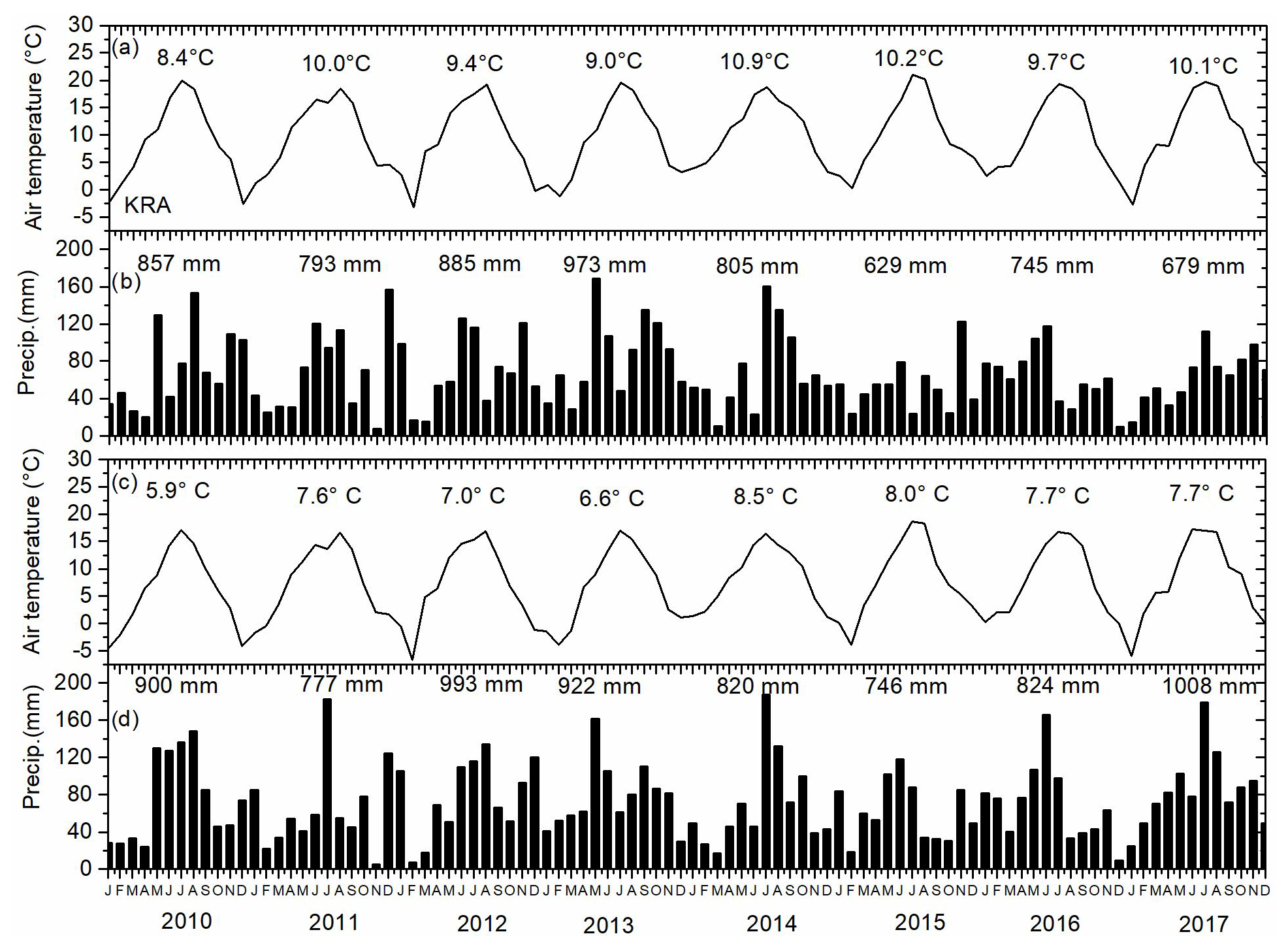
Figure 2Mean monthly air temperatures and precipitation sums at the Kraichgau site EC1 and Swabian Jura site EC4 from 2010 to 2017. Annual mean temperatures and precipitation sums are given on top of the lines or bars.

Download

Additionally, the micro-topography of the EC sites was determined along a transect in the prevailing wind direction (Fig. 1). About every two meters, the elevation of the fields above mean sea level was measured with a differential global positioning system (Altus APS 3M, Septentrio, Belgium).

2.6 Statistical analyses

For the statistical analyses, we used all available data on energy fluxes from the onset of measurements (late March or early April) until harvest. In the case of maize, however, full data for the calculation of energy balances were generally available from May. Autocorrelation of the data was tested using the Durbin–Watson test (Faraway, 2014). Analysis of variance (ANOVA) was used to test for significant effects of region, site, year, and crops on EBC, for which linear mixed models were defined (Piepho et al., 2004). The data were assumed to be normally distributed but heteroscedastic due to the different years. We based these assumptions on graphical residual analyses. Generally, the factors of interest were defined as fixed, and interaction terms were considered. Remaining factors not included in the ANOVA were defined as random. Multiple contrast tests (Bretz et al., 2011) were performed to identify significant differences between the different factor levels. Unless indicated otherwise, the significance level was set to α=0.05. Calculations were done using the statistical software R (R Core Team, 2014) and packages multcomp for simultaneous tests of linear mixed models (Hothorn et al., 2017), nlme for fitting and comparing the models (Pinheiro et al., 2016), gplots for creating plots (Gregory et al., 2009), and gdata for importing input data from files formatted by Microsoft Excel files (Gregory et al., 2017).

3.1 Meteorological and terrain conditions

3.1.1 Kraichgau

At the KR sites, the annual mean air temperature ranged between 8.4 ^∘C in 2010 and 10.9 ^∘C in 2014. The overall average was 9.8 ^∘C (Fig. 2a), which is 0.4 ^∘C higher than the 30-year climatological mean (1981–2010) measured at the meteorological station Pforzheim-Ispringen. The lowest and highest monthly mean temperature was −3.2 ^∘C in February 2012 and 21.1 ^∘C in July 2015. The mean annual precipitation was 796 mm, which is 93 mm lower than measured in Pforzheim-Ispringen. In 2013, the wettest year within the 8-year period, total precipitation amounted to 973 mm. The lowest annual precipitation (629 mm) was measured in 2015 (Fig. 2b).

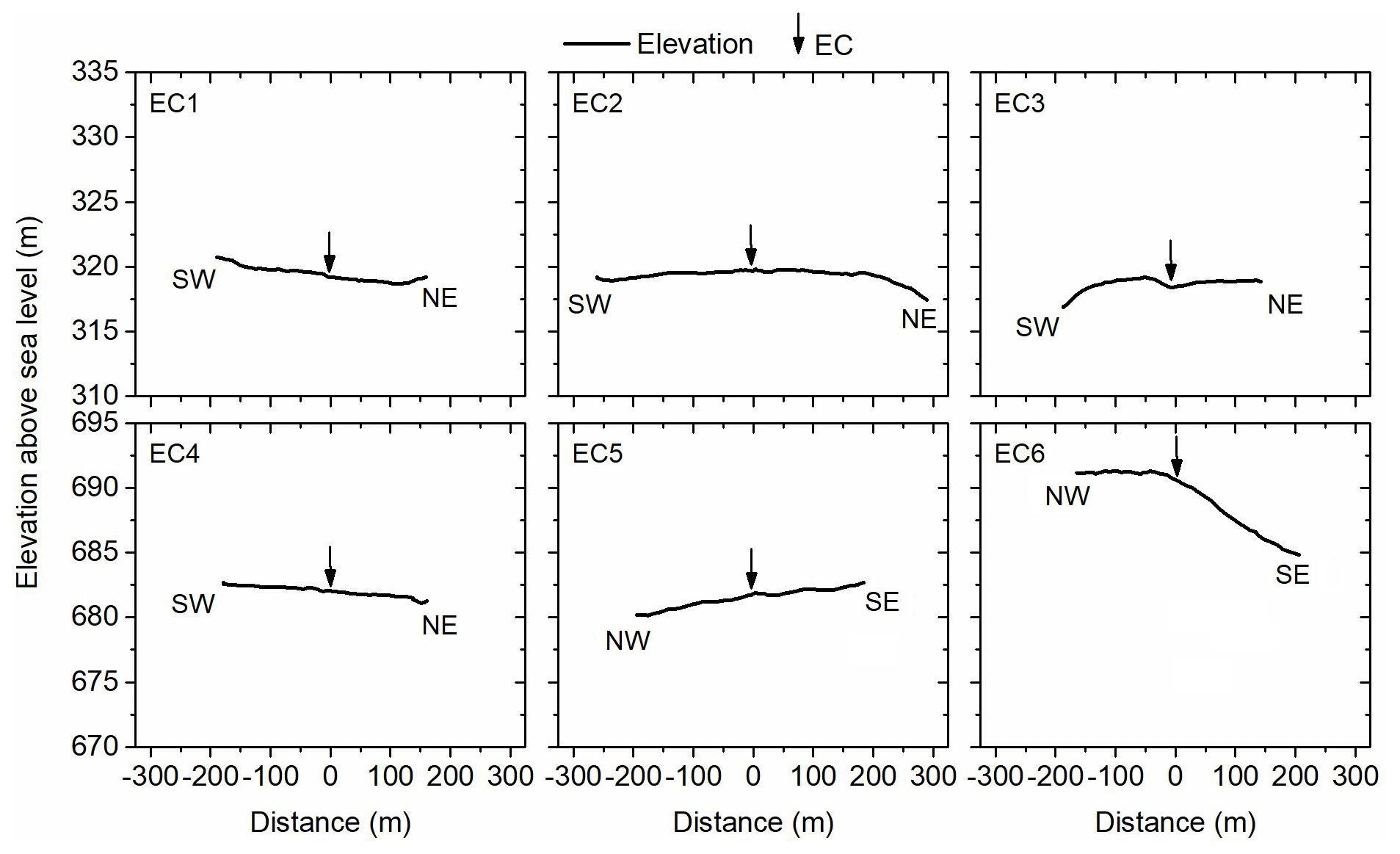
Figure 3Elevations at EC sites along the dominant wind directions (see Figs. 1 and 3). Arrows present positions of EC stations.

Download

Figure 3 shows the height transects along the prevailing wind direction. At the KR sites, the mean slopes along the transects were 0.4 %, <0.01 %, and 0.3 % at EC1, EC2, and EC3, respectively. The micro-relief of station EC1, located on a micro-bank, fluctuates more strongly than that of EC2. The immediate surroundings of EC2 are very homogeneous in elevation. Station EC3 was positioned in a micro-depression. Overall, the three transects show that the KR fields can be regarded as flat, with EC2 being the flattest.

3.1.2 Swabian Jura

The mean temperature in SJ (7.4 ^∘C) was 2.4 ^∘C lower than in KR, varying from 5.9 ^∘C in 2010 to 8.5 ^∘C in 2015 (Fig. 2c). As in KR, the lowest and highest mean monthly temperatures were recorded in February 2012 (−6.6 ^∘C) and July 2015 (18.6 ^∘C). The mean annual precipitation was 874 mm. As in KR, 2015 was the year with the lowest precipitation. Highest total rainfall was measured in 2017, not in 2013 as in KR. November 2011 was the month with the lowest monthly cumulative precipitation (5 mm), and July 2014 was that with the highest (187 mm; Fig. 2d).

In SJ, only EC4 is relatively flat (Fig. 3). Its topography is comparable with that of EC1 in KR. The elevation along the transect at EC5 gently increases, with a mean slope of 0.6 % from SE to NW. Station EC5 itself is situated in a local micro-depression. The topography of station EC6 differs considerably from that of the other fields. The station is positioned on the top of a ridge. Whereas in NW direction the terrain drops with a mean rate of 3.7 m per 100 m, in SE direction the terrain is nearly flat (slope=0.3 %).

Figure 4Diurnal courses of energy balance components averaged over 3-month periods in Kraichgau (EC1, EC2, and EC3) and Swabian Jura (EC4, EC5, and EC6) in 2016. Insets denote the different crops grown in 2016; see main text for explanation. Because of energy shortage during winter at the EC1, EC3, EC4, and EC5 sites, the fluxes shown in the JFM and OND graphs were measured only in March and from 1 October to mid-November, respectively.

Download

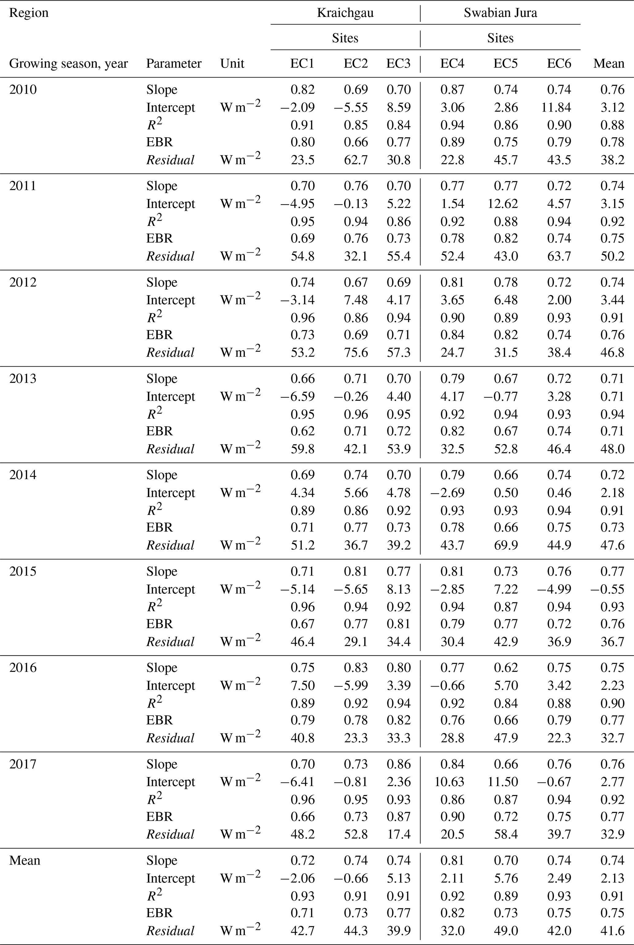
Table 3Annual mean energy balance closure (EBC; slope of linear regression) and energy balance ratio (EBR) at the eddy-covariance stations EC1 to EC6 in Kraichgau and Swabian Jura during 2010–2017. Regressions are based on half-hourly data.

Download Print Version | Download XLSX

3.2 Energy partitioning at the land surface

The energy partitioning at the canopy surface of different crop stands is shown, by way of example, for the vegetation period of 2016 (Fig. 4). In that year, five different crops (winter rapeseed – WR, spring barley – SB, winter wheat – WW, silage maize – SM, and grain maize – GM) were grown at the EC sites. From April to June, most of the net radiation was transformed into latent heat at the crop stands, except for SM at EC5. The daytime Bowen ratio was lowest for WW and WR, with 0.14 and 0.13, respectively. Also GM, SB, and SM at EC6 led to daytime Bowen ratios distinctly below unity (about 0.21). Only silage maize at EC5 had a Bowen ratio of about unity, which indicates that the available energy was partitioned into latent and sensible heat in similar proportions. For the WW, SB, and WR sites and years, the ground and sensible heat fluxes were nearly the same and showed a similar diurnal course. At the maize stands, the ground heat flux tended to be higher than the sensible heat flux during the morning hours, while in the afternoon the order switched and more sensible heat than ground heat was formed. At all sites, the measured energy residual was similar to the sensible heat fluxes, ranging from 23 W m⁻² at EC3 to 44 W m⁻² at EC1. The daily net radiation was 149, 133, 134, 130, 138, and 164 W m⁻² at EC1 to EC6, respectively. The mean daily LE ranged from 54 W m⁻² at EC5 to 94 W m⁻² at EC3.

For July to September, the strongest shift in energy partitioning occurred at the WR site. In the afternoon, the Bowen ratio was in the range of unity, and sometimes the half-hourly sensible heat flux was even higher than the latent heat flux. A similar shift was observed at the WW site, but it was weaker than at the WR site. At the GM, SM, and SB sites the largest difference compared with the period April to June was the ratio between the sensible and ground heat flux. From July to September the sensible heat was about twice the ground heat flux. The mean net radiation ranged from 125 W m⁻² at EC5 to 176 W m⁻² at EC2, and LE varied from 78 W m⁻² at EC4 to 89 W m⁻² at EC1. The residual energy for this period was 23, 28, 22, 24 and 16 W m⁻² at the sites EC1, EC2, EC3, EC4, and EC6, respectively. Note that EC5 data are missing due to damage in the sonic anemometer and gas analyzer.

3.3 Energy balance closure

The mean EBR over the 48 years on-site was 0.75, corresponding to a mean energy residual of 41.6 W m⁻² (Table 3). The mean annual EBR ranged between 0.62 at EC1 (WW in 2013) and 0.90 at EC4 (SM in 2017). The mean EBR over the six EC stations was highest in 2010 (EBR = 0.78) and lowest in 2013 (EBR = 0.71). Averaged over the period from 2010 to 2017, the best EBC was achieved at EC4 (EBR = 0.82), whereas the largest mean energy gap occurred at the neighboring station EC5. There, the mean residual was 49.0 W m⁻².

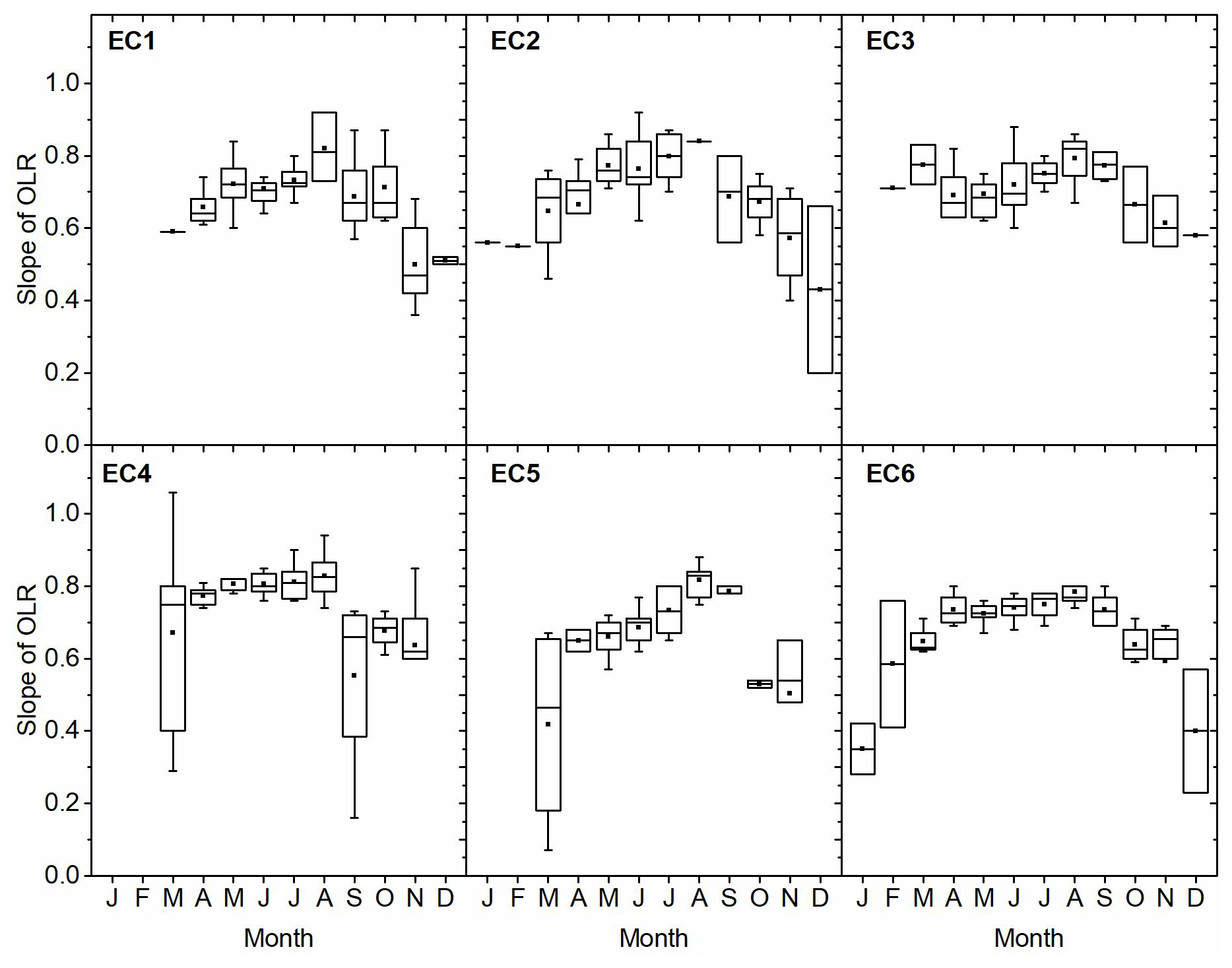
Figure 5Monthly aggregated energy balance closure (EBC) obtained by ordinary linear regression of turbulent fluxes (LE+H) against available energy (R_n−G) for all stations during 2010–2017.

Download

Figure 5 presents the course of monthly mean EBC determined by the OLR for all six stations averaged over the period 2010–2017. In general, the EC method performed best (EBC was highest) over the vegetation period from April to August. The highest EBC was usually found during July and August and distinctly declined over autumn and winter. At station EC6, the SJ station equipped with a fuel cell system, for example, the EBC declined to 42 % in January 2016 and 23 % in December 2017. A low EBC was usually associated with a larger variation (see winter months; Fig. 5).

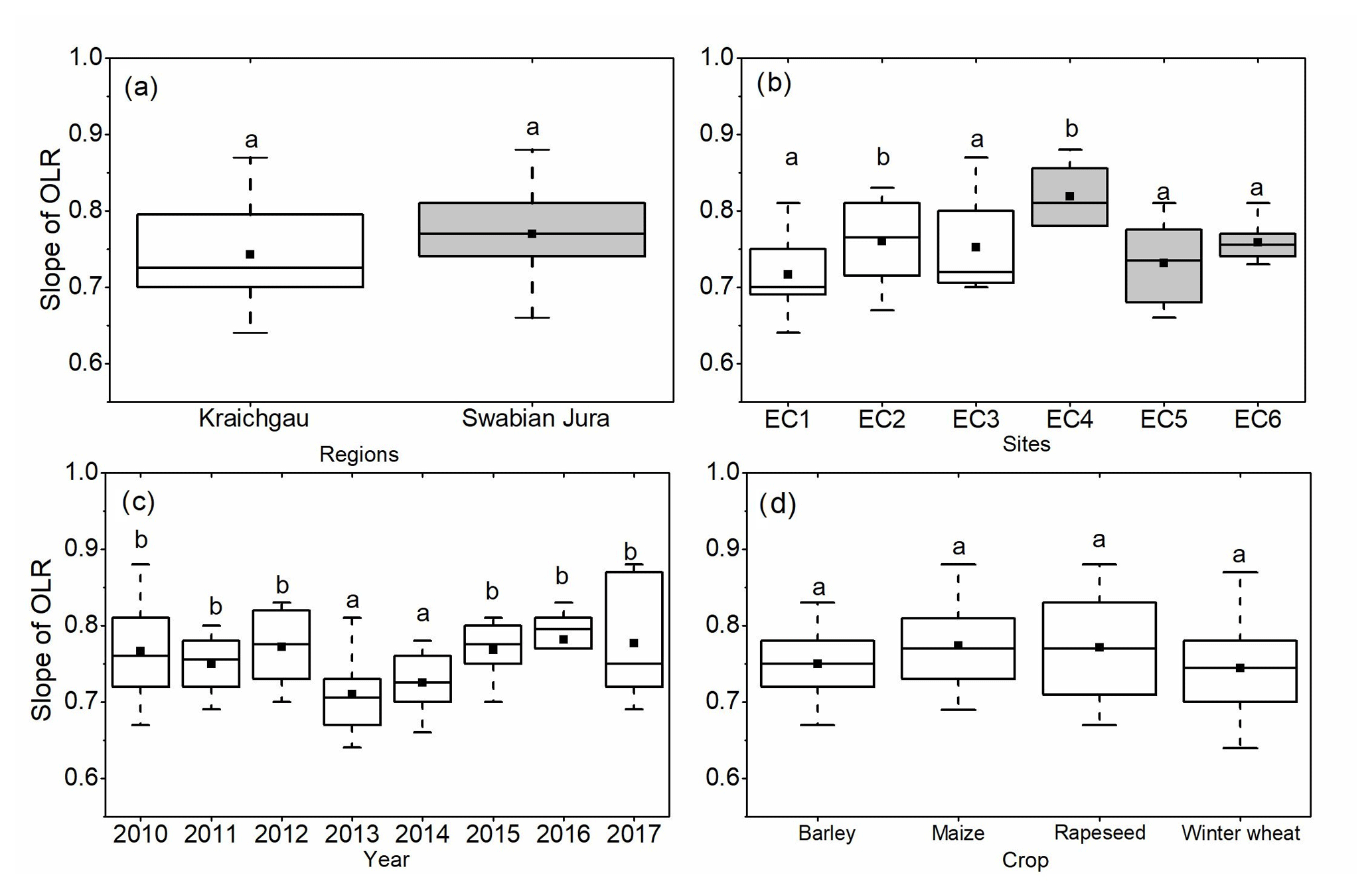
Figure 6Comparison of energy balance closure (EBC) measured by linear regression, grouped for the different regions, sites, years, and crops. Measurements were conducted from early spring until harvest. Different letters indicate significant (a – insignificant, b – significant) differences between the factor levels at α=0.05.

Download

3.4 What impacts the EBC?

3.4.1 Effect of region, station, year, and crop

The statistical analyses showed that the EBC over the main vegetation period from early April until harvest did not differ between the two regions (Fig. 6a). The EBC was significantly higher at stations EC2 and EC4 (p<0.001; p – probability level) than at the other stations (Fig. 6b). The lowest spread in values was observed at station EC4. In 2013 and 2014, EBC was lower (p<0.001) than in the other 6 years (Fig. 6c). The crops had no significant effect on mean EBC (Fig. 6d). EBC over winter rapeseed showed the highest variation in comparison to the other four crops, varying between 57 % and 88 %.

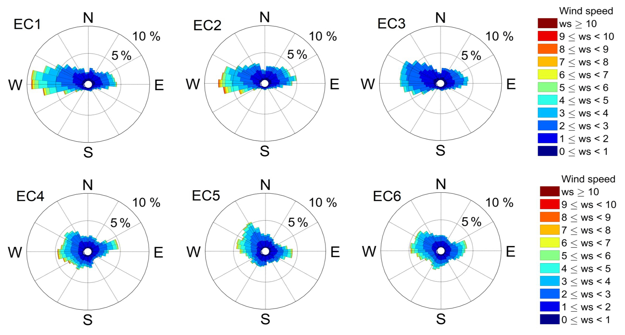
Figure 7Distribution of wind direction and wind speed (m s⁻¹) from 2010 to 2017 in Kraichgau (EC1–EC3) and Swabian Jura (EC4–EC6).

Download

3.4.2 Effect of wind speed and direction

Typical for the midlatitudes, the KR sites' prevailing wind direction was from west to east. The fraction of WSW to WNW (240–300^∘) winds was 43.2 %, 36.8 % and 33.7 % at EC1, EC2, and EC3, respectively (Fig. 7). The highest wind speeds were also measured within these wind direction sectors. Wind blowing from north- and southward directions was rarely measured (<10 %). While at EC1 the wind speed averaged 2.9 m s⁻¹, at EC2 and EC3 the values were 2.4 and 1.9 m s⁻¹, respectively. Moreover, high wind speeds (>6 m s⁻¹) clearly decreased from the most westerly station (EC1) to the most easterly station (EC3). At EC1, EC2, and EC3, the share of these high wind speeds was 4.6 %, 3.3 %, and 0.2 %, respectively.

In SJ, the wind blew mostly from westerly or easterly directions (Fig. 7). The wind from the 240–300^∘ sector was less than in KR, with shares of 14.4 %, 25.5 %, and 26.6 % at EC4, EC5, and EC6, respectively. At EC5, more wind was recorded from the NW sector (300–330^∘). Mean horizontal wind speeds at EC4, EC5, and EC6 were 2.44, 2.38, and 2.51 m s⁻¹, respectively. Wind speeds above 6 m s⁻¹ made up 2.0 (EC4), 1.7 (EC5), and 1.3 % (EC6) of all measured wind speeds in SJ.

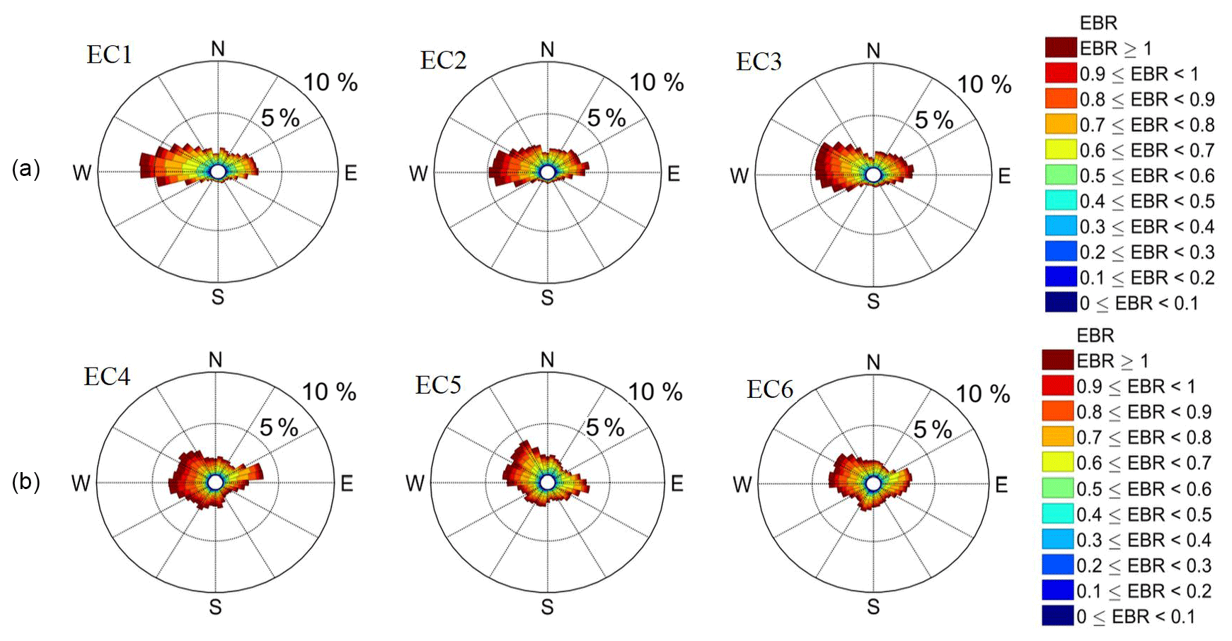
Figure 8Distribution of half-hourly energy balance ratios (EBR) in terms of wind direction at eddy-covariance (EC) stations during the 2010–2017 study period. Spike lengths in diagram show relative frequency of wind directions; color of legend shows EBR. This is shown for (a) Kraichgau and (b) Swabian Jura.

Download

The distribution of the EBR as a function of wind direction is shown in Fig. 8. The EBR was averaged for 30^∘ wind sectors over all available daytime data (global radiation >10 W m⁻²). At the KR sites, the highest EBR was achieved when the wind blew from westerly directions, which is the prevailing wind direction. Wind from northern and southern directions was related to a lower EBR. Particularly wind from the south was associated with an EBR below 0.6 at all three stations. This phenomenon was most pronounced at station EC1. Also at the SJ sites, the highest EBR usually coincided with wind from the prevailing direction. One exception is the high EBR at EC4 for the south–southeast sector. At EC4, for six out of the 12 wind sectors, EBR was above 0.8. In contrast, at EC5 and EC6, the EBR exceeded 0.8 in only three wind sectors. At all stations, the EBR was lowest (<0.6) for winds from the northeast (Fig. 9).

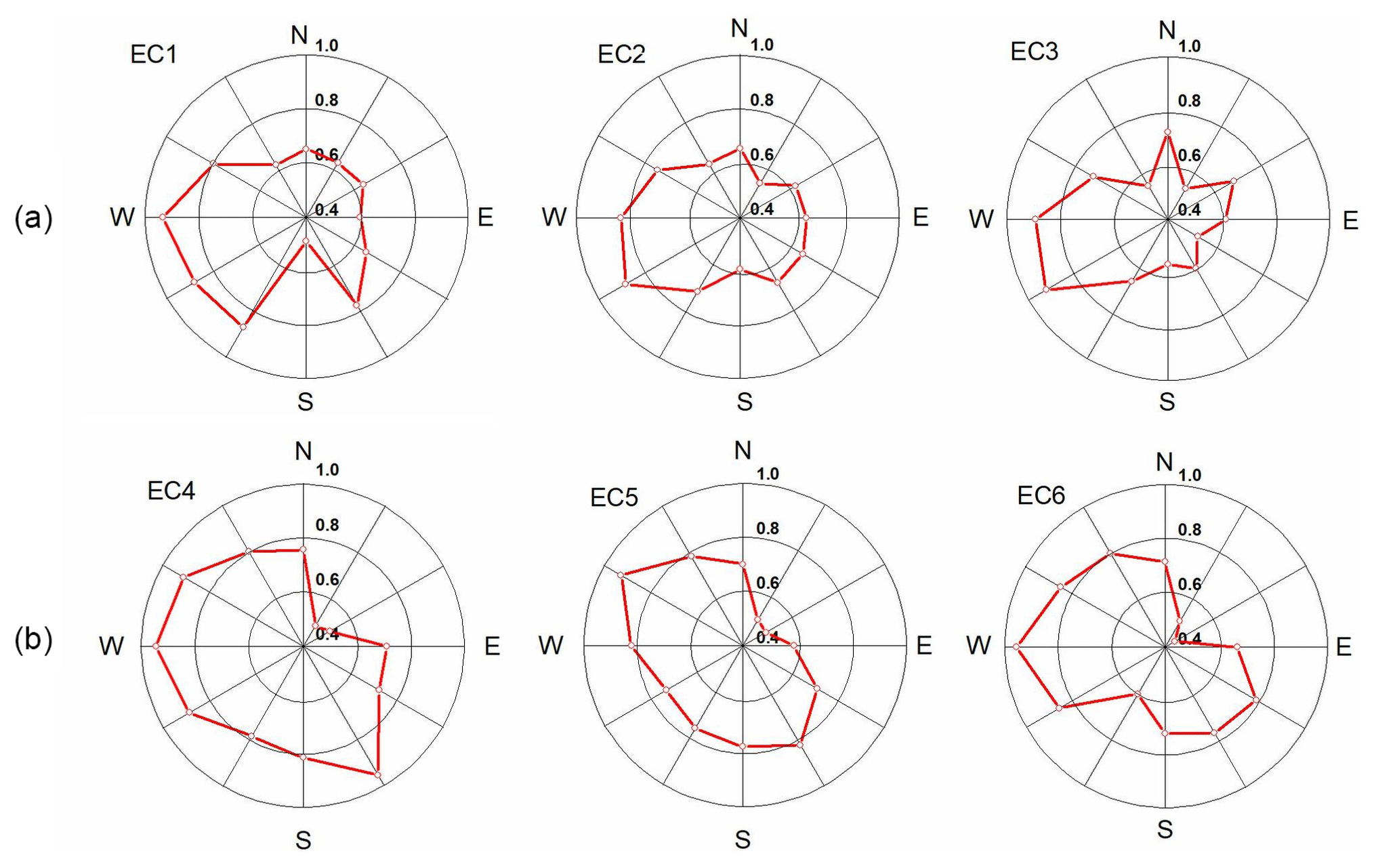
Figure 9Half-hourly energy balance ratio (EBR) averaged for 30^∘ wind sectors at the six eddy-covariance (EC) stations during the 2010 to 2017 study period. This is shown for (a) Kraichgau and (b) Swabian Jura.

Download

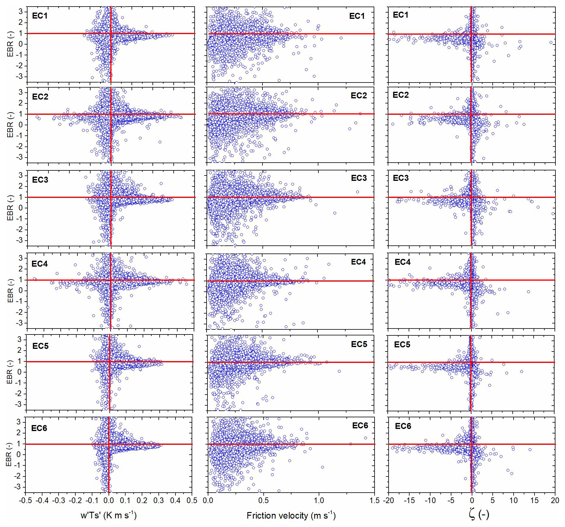
Figure 10The mean energy balance ratio (EBR) as a function of buoyancy flux ($w^{\prime }{T}_{\mathrm{s}}^{\prime })$, friction velocity (u^*), and the stability parameter (ζ) during the 2010–2017 study period.

Download

3.4.3 Effect of atmospheric conditions

This section evaluates the EBR as a function of buoyancy, shear, and atmospheric stability. For this purpose, we plotted the EBR against the kinematic virtual temperature flux ($w^{\prime }{T}_{\mathrm{v}}^{\prime }$, proxy for buoyancy), friction velocity (u^∗, proxy for shear), and the stability parameter ζ (Fig. 10). Again, only half-hourly daytime fluxes (R_s>10 W m⁻²) were evaluated. The plot EBR versus $w^{\prime }{T}_{\mathrm{v}}^{\prime }$ shows a vast scatter at weak buoyancy. Here, the EBR ranges from plus four to minus four. The scatter decreases substantially as the modulus of $w^{\prime }{T}_{\mathrm{v}}^{\prime }$ increases. Note that $w^{\prime }{T}_{\mathrm{v}}^{\prime }\mathit{<}-\mathrm{0.15}$ K m s⁻¹ were measured only at stations EC2 and EC4.

Plotting the EBR against friction velocity also reveals a large scatter, which narrows as friction velocity (shear) increases. The scatter, however, does not narrow as much as for increasing buoyancy. During neutral or stable atmospheric conditions, the EBR showed a large spread (Fig. 10). In contrast, this range distinctly declined when the stability parameter reached strongly negative values, indicative of highly unstable conditions. An EBR above unity or below zero was rarely observed under these conditions.

Table 4Energy balance closure (EBC) as indicated by the slope of linear regression of turbulent vs. available energy and energy balance ratio (EBR) under different atmospheric stability conditions. EBC and EBR are given as site-specific averages from 2010 to 2017. SD is standard deviation.

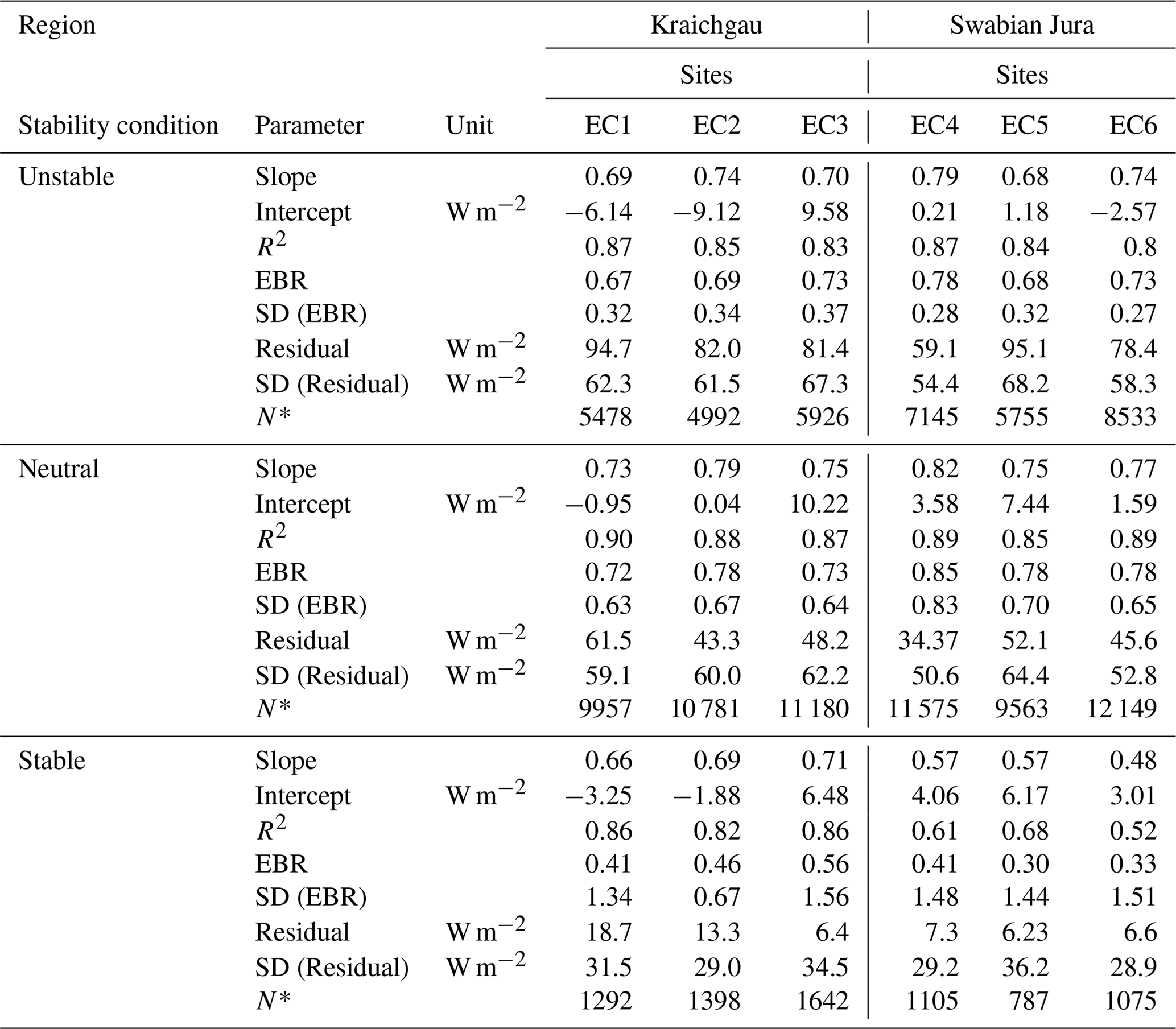
* Number of data points.

Download Print Version | Download XLSX

From the total dataset, only 7 % of daytime measurements were made under stable conditions, 34 % under unstable conditions, and 59 % under neutral conditions (Table 4). During unstable conditions, the EBC and EBR at all sites were slightly lower compared to neutral conditions. During neutral conditions, however, the standard deviation (SD) of EBR was about twice as high as under unstable conditions. During stable conditions, the EBC and EBR were systematically lower than at unstable and neutral conditions. At EC4, for example, the EBR was 0.78 and 0.85 under neutral and unstable conditions, respectively. Under stable conditions, the value declined to 0.41. Moreover, the huge spread in the EBR under stable conditions is underlined by its high SD, which is about 3 times the mean value.

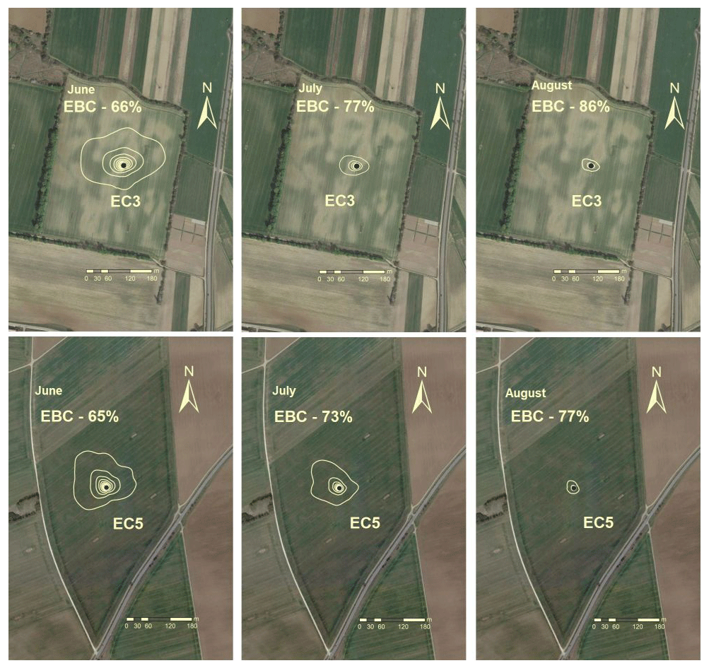
Figure 11Footprint area of EC3 and EC5 in selected months of 2015 and the corresponding energy balance closure (EBC). Black points represent positions of EC stations. Yellow lines indicate relative areal contributions to total flux in 10 % steps, where the outmost yellow line indicates the area from which 90 % of measured fluxes originated. The satellite image was taken from Google Earth (images from 31 March 2017 and 30 March 2014 for EC3 and EC5, respectively).

Download

4.1 EBC and energy balance components

From July to September, daily mean R_n varied between 125 and 176 W m⁻². Similar ranges of R_n were observed over maize in Livraga, Italy (Masseroni et al., 2014). The latent and sensible heat fluxes varied strongly over the observational period. In early covering crops (winter rapeseed, winter wheat, and winter barley), LE was about 2 to 3 times higher than H in the period AMJ (April–May–June), while in the period JAS (July–August–September), LE and H were in a similar range (Fig. 4; EC3-WW, EC4-SB). The period JAS is when the ripening and harvest of cereals and winter rapeseed occurs as well as post-harvest management such as tillage and seeding of cover crops or winter rapeseed. During AMJ, the patterns of LE and H at EC5 and EC6 differed, even though the maize was sown on similar days of the year (7 May at EC5 and 3 May at EC6). This can be explained by the substantially higher leaf area index at EC6 (0.74±0.15) compared to EC5 (0.35±0.06), measured on 22 June.

The mean EBR of the 48 years on-site was 0.75 (Table 3). In comparison, Wilson et al. (2002) reported an EBR of 0.84, on average, for the 50 analyzed FLUXNET years on-site, ranging from 0.34 to 1.69. In three agricultural and one industrial site in South Korea, the mean value varied between 0.46 and 0.83 (Kim et al., 2014). Majozi et al. (2017) found a mean EBR of 0.93 at a semi-arid savannah site in South Africa, over a period of 15 years.

The slopes of the OLR and EBR differed by a maximum of 5 %, which is consistent with previously published data. Such a small difference points to a high reliability of the presented EC measurements (Wilson et al., 2002). The highest annual EBC occurred at EC4 (87 % in 2010), the second highest at EC2 (83 % in 2016), and the lowest at EC5 (62 % in 2016). The lowest EBC was observed mainly in the cold, non-growing season, which may be attributed to insufficient thermally and mechanically induced turbulence (Franssen et al., 2010) as well as to freezing (Varmaghani et al., 2016).

The incomplete EBC in our dataset has several potential explanations. One is related to the neglected minor storage terms (Eshonkulov et al., 2019; Masseroni et al., 2014; Meyers and Hollinger, 2004). Importantly, considering minor storage terms is not straightforward, because they are not measured when conventional EC equipment is used. Only the energy fixed and released by photosynthesis and respiration can be directly derived from EC data, because the net CO₂ flux is generally measured. Considering minor storage terms in calculating the EBC at a maize field improved the mean value from 87 % to 91 % (Xu et al., 2017) and from 81 % to 86 % (Masseroni et al., 2014). Eshonkulov et al. (2019) demonstrated that the contribution of minor storage and flux terms over winter wheat in southwestern Germany was largest during the main vegetation period in May. During this month the minor terms helped to close the energy balance by an additional 7 %–8 %.

4.2 The effect of meteorological conditions and surface-layer turbulent parameters

In both KR and SJ, the EBR was highest for winds blowing from the prevailing wind direction. These winds were associated with high wind speeds favoring well-developed turbulent conditions. This is consistent with other studies. Xin et al. (2018), for example, also found that winds with high speeds blowing from the prevailing direction yielded consistently higher EBC compared to other directions. Kim et al. (2014), for example, grouped EBR into two different categories, one with a lower EBR (<0.75) and one with a higher EBR (>0.75), and observed for their four research sites that the EBR was higher at high wind speed.

Figure 10 shows that the spread of the EBR distinctly narrowed at high friction velocities ($u^{*}\ge \mathrm{0.5}$). Prior studies have noted the importance of u^* on the EBC. Anderson and Wang (2014) found that, under these conditions, EBC was closed on days with continuous turbulence. Results of the hourly daytime EBR and u^* showed a strong relationship at our sites (Fig. 10). This is consistent with other studies carried out in selected croplands such as irrigated sugarcane (Anderson and Wang, 2014), maize plantations (Masseroni et al., 2014), and rice fields (Kim et al., 2014). Sánchez et al. (2010) also reported that EBR was >0.90 when high friction velocities prevailed (>0.8 m s⁻¹) at a boreal forest site in Finland. Mauder et al. (2013) investigated EBC at the TERENO site in Lackenberg (Germany) and found that it was almost closed. They explain this result by the very good turbulent mixing and the high homogeneity at this site. This confirms that, at high u^*, the production of high-frequency fluxes is elevated (Fratini and Mauder, 2014).

At our study sites, neutral conditions dominated (∼60 %), followed by unstable conditions (∼34 %) and stable conditions (6 %; Table 4). Importantly, average EBR changed from 0.67 (±0.32) to 0.72 (±0.69) and 0.41 (±1.33) during unstable, neutral, and stable conditions, respectively (SD in brackets). Under stable conditions, the EBR was lowest and had the largest variation. Averaged over all EC stations, the slope of OLR under neutral conditions was slightly higher than under unstable conditions. This is also evident in the mean and variance of the calculated energy residuals. The average residuals under stable, neutral, and unstable conditions were 9.7 (±31.5), 47.5 (±58.2), and 81.5 (±62.0) W m⁻², respectively. The coefficient of variation was highest under stable conditions and decreased over neutral to unstable conditions. This result differs from previous studies. Mauder et al. (2010) reported a residual energy close to zero for a cropland in Ontario, Canada, under stable conditions, peaking at 150 W m⁻² under neutral conditions and decreasing to 100 W m⁻² under unstable conditions.

The scatter of EBR versus buoyancy flux at EC2 and EC4, the two stations with the highest EBC, differed from those of the other stations (Fig. 10). At these two sites, strong negative buoyancy fluxes below −0.15 K m s⁻¹ were recorded. This means that the atmosphere was not heated by the land surface but that the land surface was significantly heated by the atmosphere. Such a situation points to a stable boundary layer (SBL). Lan et al. (2018) report that they measured the highest buoyancy fluxes under a weak SBL with strong surface shear. They argue that the strong mechanical shear produced at the ground favors the development of turbulent eddies with larger scales that enhance vertical mixing of momentum and heat transporting the warm air aloft downward and the surface cold air upward. Moreover, the mechanical mixing weakens the magnitude of the mean temperature gradient and allows turbulent eddies with larger vertical scales to develop. Conversely, under a SBL, weak winds occur near the surface, and turbulent eddies are depressed and detached from the boundary leading to suppressed vertical mixing.

Several studies recommended considering secondary circulations to achieve a better EBC (Foken et al., 2010; Kidston et al., 2010; Mauder et al., 2010). Those studies postulate that heterogeneity-induced and buoyancy-driven quasi-stationary circulations are probably the dominant processes behind underestimated energy fluxes. The studies that suggested the use of an averaging period higher than 30 min usually refer to unstable conditions. These studies suggested that averaging periods of 2–4 h are often needed to statistically resolve the largest convective turbulent eddies or also non-stationary mesoscale motions that sometimes can modulate turbulent fluxes (Mahrt, 1998). Larger averaging improved short-term EBC during the diurnal hours in the Salentum peninsula of Apulia, Italy (Cava et al., 2008). In considering secondary circulations, different time averaging intervals can be used instead of the standard 30 min period. Although a 60 min interval might be suitable for capturing the major turbulent fluxes (Kilinc et al., 2012), in most cases the standard 30 min period is still sufficient (Kidston et al., 2010). The classical averaging period of 30 min can be a proper choice for unstable or neutral conditions. A shorter averaging period is suitable for capturing energy fluxes in very stable conditions (Sun et al., 2012; Vickers and Mahrt, 2006). Finding an optimum averaging period is a very complex and nearly impossible task. This is because atmospheric turbulence changes irregularly, and there is no clear-cut “switch” in time. Therefore, the averaging time could be modified during raw data processing. In practice, however, this is unlikely, because it drastically increases the complexity of data processing (Lenschow et al., 1994). Moreover, the sources of secondary circulations are unclear, and they are most probably not well linked with the locally measured available energy. Accordingly, excluding secondary circulations in EC measurements can be locally meaningful. Recently, a new method, known as ogive optimization, was proposed by Sievers et al. (2015). The method enables the separation of low-frequency influences from vertical turbulent fluxes for isolating the local exchange processes of interest.

Although EC measurements contain uncaptured energy components, the flux data are used, among others, to evaluate models and interpret simulation results. In such studies, EC flux data are usually post-closed, i.e., the measured turbulent fluxes are adjusted so as to close the energy balance (Ingwersen et al., 2015). The standard approach is the Bowen-ratio post-closure method (Twine et al., 2000). It assumes that the missing energy has the same Bowen ratio as the measured turbulent fluxes. This approach, however, may introduce a systematic bias to simulated surface energy fluxes (Chen and Li, 2012). Analyses of the energy imbalance by Ingwersen et al. (2011) showed that soil water contents simulated by a land surface model agreed better with measurements when the residual was fully assigned to H. As discussed by Charuchittipan et al. (2014), secondary near-surface circulations attributed to low frequencies mainly transport sensible heat. Therefore, they proposed a new alternative energy balance correction method they termed the Buoyancy flux ratio. At very large Bowen ratios (>10), the Bowen-ratio post-closure and buoyancy flux correction methods yield similar results. At Bowen ratios ranging from 0.1 to 0.2, which are typical for croplands during the main growing period, the Buoyancy flux ratio method assigns most of the energy residual (>50 %) to the sensible heat flux. The Bowen-ratio method, in contrast, distributes most of it (>90 %) to latent heat. As long as the composition of the residual remains unknown, it is important to communicate the possible error in EC flux data, for example with the post-closure method uncertainty band (PUB; Ingwersen et al., 2015). Working with only one post-closure method may result in serious misinterpretations in model–data comparisons (Ingwersen et al., 2018).

4.3 The effect of the instrumental setup

At the SJ sites, we found a particularly low EBR in the wind sector 0–90^∘. The CSAT3 sensor was oriented mostly to 225^∘ so that the sector 30–90^∘ was located behind the anemometer head. To substantiate the idea that the anemometer negatively influences EC measurement quality, and taking the data from EC4 as an example, we recalculated EBR across all years, excluding the wind directions of the sector 0–90^∘. This increased the mean EBC in 2010–2017 by 4 percentage points, from 80 % to 84 % (data not shown). Friebel et al. (2009) used a wind tunnel experiment to show that there is a 40^∘ shadow zone behind the sonic anemometer where the measured wind speeds were reduced by up to 16 %. Within a shadow zone of about 20^∘ behind the anemometer, the turbulent spectra were corrupted. Our findings indicate that under field conditions the shadow zone was even somewhat wider (about 60^∘). A practical solution for measuring reliable fluxes when winds blow from the back of the anemometer could be to operate an anemometer tandem: a first anemometer orientated in the prevailing wind direction and a second one in the opposite direction. Whether this setup could solve the problem requires further investigation.

4.4 Relationships between EBC and footprint

Accurate measurements of energy balance components are important to achieve a good EBC. In this context, one key requirement is that the EC station be located in a place that represents the fluxes from the area of interest (Burba and Anderson, 2010). According to those authors, the terrain must be horizontal and uniform. Three parameters are needed in footprint analysis: measurement height, surface roughness, and atmospheric stability. When turbulent fluxes originate from a horizontal and homogeneous surface, the footprint depends solely on the distance between the location of the measurement point and the emission element. We found a distinct tendency that the smaller the footprint, the higher the EBC. We give two explanations. First, the smaller the footprint, the higher the chance that the assumption of a homogeneous source area is fulfilled. Second, the smaller the footprint, the better the scale match between the measurement of available energy and turbulent fluxes. Alfieri and Blanken (2012) found that variations of surface energy fluxes over tens of meters ranged from 30 to 40 W m⁻² using single-point (immobile) and mobile EC towers at a uniform site (Colorado, USA). They concluded that a single-point EC tower cannot capture all the relevant energy fluxes, because they vary spatially. Our results confirm that if the footprint is small, the EBC from EC measurements is better, which can be interpreted as a reduction in the variation of surface energy fluxes.

Many studies claimed that surface heterogeneity is a potential reason for the energy imbalance (Stoy et al., 2013; Xu et al., 2017). The latter authors reported that EBC decreased with increasing surface heterogeneity. The degree of heterogeneity was derived from high-resolution remote sensing images and land surface temperatures. To handle this effect, some authors recommend using direction-specific coefficients that indicate the degree of heterogeneity. For example, Panin et al. (1998) introduced a heterogeneity factor that comprises surface parameters such as roughness, radiation, and the thermal humidity of the internal boundary layer. That factor can be used for data interpretation. Nonetheless, deploying heterogeneity factors still does not explain how the residual energy is composed. The lack of EBC at the KR sites might partly reflect katabatic advection (Heinesch et al., 2008; Kutsch et al., 2008), which results from stable atmospheric conditions and occurs especially in hillslope areas (Loescher et al., 2006; Mauder et al., 2010). Moreover, complex topography can induce advective fluxes (Feigenwinter et al., 2008; Rebmann et al., 2010). The former landfill site located about 500 m south of the fields in KR (Fig. 1) might have been responsible for advective fluxes, since its elevation is approximately 41 m higher than the study sites. Moreover, the topography could also affect EBC. The elevation transects show that the immediate terrain surrounding the stations EC3, EC5, and EC6 is not totally flat (Fig. 4). This is a well-known problem for micrometeorological field measurements (Wilczak et al., 2001). At EC1, EC2, and EC4, however, the terrain can be considered flat.