the Creative Commons Attribution 4.0 License.
the Creative Commons Attribution 4.0 License.
 | 16 Dec 2019
Long-term trends in pH in Japanese coastal seawater
Yasumasa Miyazawa
Tomohiko Tsunoda
Tsuneo Ono
In recent decades, acidification of the open ocean has shown a consistent increase. However, analysis of long-term data in coastal seawater shows that the pH is highly variable because of coastal processes and anthropogenic carbon inputs. It is therefore important to understand how anthropogenic carbon inputs and other natural or anthropogenic factors influence the temporal trends in pH in coastal seawater. Using water quality data collected at 289 monitoring sites as part of the Water Pollution Control Program, we evaluated the long-term trends of the pHinsitu in Japanese coastal seawater at ambient temperature from 1978 to 2009. We found that the annual maximum pHinsitu, which generally represents the pH of surface waters in winter, had decreased at 75 % of the sites but had increased at the remaining sites. The temporal trend in the annual minimum pHinsitu, which generally represents the pH of subsurface water in summer, also showed a similar distribution, although it was relatively difficult to interpret the trends of annual minimum pHinsitu because the sampling depths differed between the stations. The annual maximum pHinsitu decreased at an average rate of −0.0024 yr−1, with relatively large deviations (0.0042 yr−1) from the average value. Detailed analysis suggested that the decrease in pH was caused partly by warming of winter surface waters in Japanese coastal seawater. The pH, when normalized to 25 ∘C, however, showed decreasing trends, suggesting that dissolved inorganic carbon from anthropogenic sources is increasing in Japanese coastal seawater.
- Article
(5469 KB) -
Supplement
(853 KB) - BibTeX
- EndNote


The effect of ocean acidification on several marine organisms, including calcifiers, is widely acknowledged and is the topic of various marine research projects worldwide. Chemical variables related to carbonate cycles are monitored in several ongoing ocean projects to determine whether the rate of ocean acidification can be identified from changes in pH and other variables in the open ocean (Gonzalez-Davila et al., 2007; Dore et al., 2009; Bates, 2007; Bates et al., 2014; Midorikawa et al., 2010; Olafsson et al., 2009; Wakita et al., 2017). Analysis of pH data measured in situ at the European station in the Canary Islands (ESTOC) in the North Atlantic from 1995 to 2003 and normalized to 25 ∘C showed that the pH25 decreased at a rate of 0.0017±0.0005 yr−1 (Gonzalez-Davila et al., 2007). Similarly, analysis of the Hawaii Ocean Time series (HOT) (Dore et al., 2009) and the Bermuda Atlantic Time Series Study (BATS) (Bates, 2007) showed that the pH at ambient (in situ) sea surface temperature (pHinsitu) decreased by 0.0019±0.0002 and 0.0017±0.0001 yr−1 from 1988 to 2007 and from 1983 to 2005, respectively. Analysis of data collected along the hydrographic observation line at 137∘ E in the western North Pacific by the Japanese Meteorological Agency (JMA) (2008) showed that the pH25 decreased by 0.0013±0.0005 yr−1 in summer and 0.0018±0.0002 yr−1 in winter from 1983 to 2007 (Midorikawa et al., 2010). The winter pHinsitu in surface water in the Nordic seas decreased at a rate of 0.0024±0.0002 yr−1 from 1985 to 2008 (Olafsson et al., 2009). This rate was somewhat more rapid than the average annual rates calculated for the other subtropical time series in the Atlantic Ocean, BATS, and ESTOC and was attributed to the higher air–sea CO2 flux and lower buffering capacity (higher Revelle factor) (Olafsson et al., 2009). Wakita et al. (2017) estimated that the annual and winter pHinsitu at station K2 in the subarctic western North Pacific decreased at rates of 0.0025 and 0.0008 yr−1, respectively, from 1999 to 2015. The lower rate in winter was explained by increases in dissolved inorganic carbon (DIC) and total alkalinity (Alk) that resulted from climate-related variations in ocean currents.
These long-term time series from various sites in the open ocean indicate consistent changes in surface ocean carbon chemistry, which mainly reflect the uptake of anthropogenic CO2, with consequences for ocean acidity. Coastal seawater, however, differs from the open ocean as they are subjected to multiple influences, such as hydrological processes, land use in watersheds, nutrient inputs (Duarte et al., 2013), changes in the structure of ecosystems caused by eutrophication (Borges and Gypens, 2010; Cai et al., 2011), marine pollution (Zeng et al., 2015), and variations in salinity (Sunda and Cai, 2012).
Duarte et al. (2013) hypothesized that anthropogenic pressures would cause the pHinsitu of coastal seawater to decrease (acidification) or increase (basification), depending on the balance between the atmospheric CO2 inputs and watershed exports of alkaline compounds, organic matter, and nutrients. For example, in Chesapeake Bay, the pHinsitu has shown temporal variations over the last 60 years, presumably because of the combined influence of increases and decreases in pHinsitu in the mesohaline and polyhaline regions of the main part of the bay, respectively (Waldbusser et al., 2011; Duarte et al., 2013).
These processes that occur only in coastal regions might cause increases or decreases in the rate of acidification, meaning that the outcomes for coastal ecosystems in different regions will vary. At present we have limited information about long-term changes in pH in coastal seawater, mainly because of the difficulty involved in collecting continuous long-term data from coastal seawater around an entire country at a spatial resolution that sufficiently covers the high regional variability in coastal pH.
The Water Pollution Control Law (WPCL) was established in 1970 to deal with the serious pollution of the Japanese aquatic environment in the 1950s and 1960s. Several environmental variables, including pHinsitu, have been continuously measured in coastal waters since 1978, using consistent methods enacted in the monitoring program under the leadership of the government, to help protect coastal water and groundwater from pollution and retain the integrity of water environments. The errors in pH measurements collected in this program were assessed as outlined in the Japanese Industrial Standard (JIS) Z8802 standard protocol (2011) that corresponds to the ISO 10523 (ISO; International Organization for Standardization) standard protocol. Compared with the specialized oceanographic protocols described in the United States Department of Energy Handbook (1994), it is not difficult to achieve the JIS protocol. The JIS and DOE standard protocols allow measurement errors of less than ±0.07 and ±0.003, respectively, for the glass electrode method, and the DOE protocol demands a precision of ±0.001 for the spectrophotometric method. Measurements are generally made with the higher-quality spectrophotometric method during major oceanographic studies (e.g., Midorikawa et al., 2010).
Regardless of any shortcomings, the WPCL coastal monitoring program in Japan includes more than 2000 monitoring sites that cover most parts of the coastline (Fig. 1), so the dataset provides the opportunity to estimate the overall trend in pH in Japanese coastal areas and the regional variability in the trends from data of known precision. Suitable analytical methods could make up for these shortcomings of the WPCL dataset. In this study, we focused on the general characteristics of the overall pH trends at all monitoring sites rather than examining the trend in pH at each site in detail, after carefully considering the accuracy of the dataset.
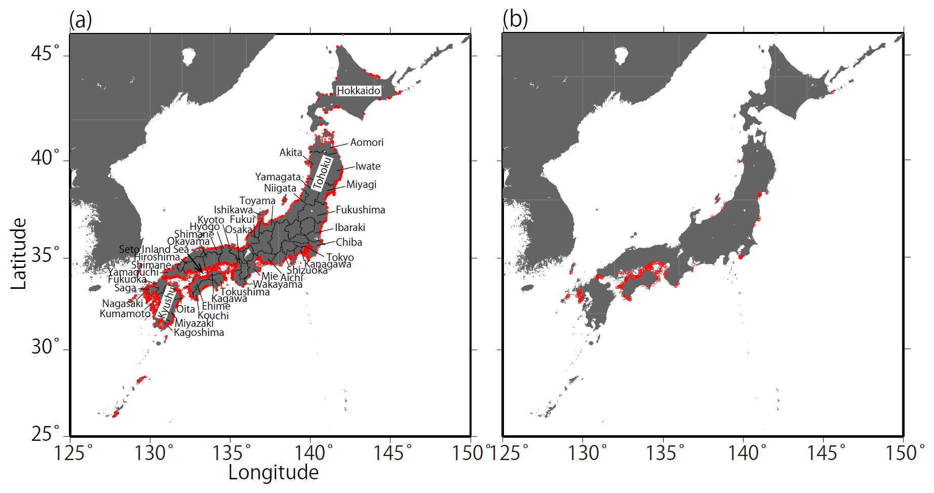
Figure 1Coastal maps and monitoring sites in Japan. Red points in (a) indicate the fixed sites (n=1481) monitored by the Regional Development Bureau of the Ministry of Land, Infrastructure, Transport, and Tourism and the Ministry of the Environment (Japan) under the WPCL monitoring program. (b) Monitoring sites that met the strictest criterion (n=302).
In the present study, we examined the pHinsitu trends in surface coastal seawater from data measured as part of WPCL monitoring programs. We then examined the trends at specific locations. The remainder of this paper is organized as follows: the data and methods are described in Sect. 2, trends in pHinsitu are presented in Sect. 3, the results are discussed in Sect. 4, and the concluding remarks are provided in Sect. 5.
2.1 Water Pollution Control Law (WPCL) monitoring data
Data for several environmental variables, including pHinsitu, and the associated metadata, are available on the website of the National Institute for Environmental Studies (NIES) (http://www.nies.go.jp/igreen, last access: 5 December 2019; http://www.nies.go.jp/igreen/md_down.html, last access: 5 December 2019). We downloaded pHinsitu data from 1978 to 2009 for the trend analysis. We also downloaded temperature (T) and total nitrogen (TN) data that were measured at the same sites as the pHinsitu data for the same time period (data for T and TN were available from 1981 to 2006 and from 1995 to 2009, respectively) to check the quality of the pHinsitu data (Sect. 2.2).
The data were collected by the Regional Development Bureau of the Ministry of Land, Infrastructure, Transport, and Tourism and the Ministry of the Environment under the WPCL monitoring program. Monitoring protocols (sampling frequencies, locations, and methods) are outlined in the program guidelines (NIES, 2018, informed by the Ministry of Environment, MOE), originally published in Japanese, and we have provided a summary of these protocols in this paper.
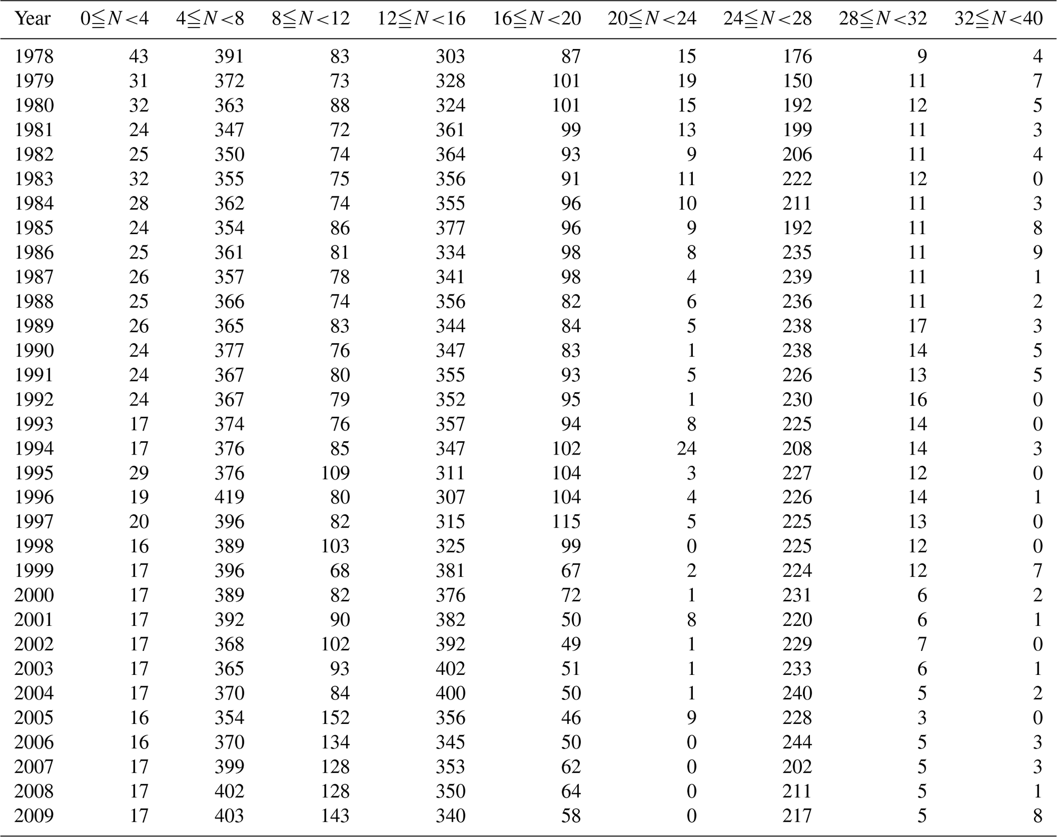
Monitoring is carried out at 1481 sites along the Japanese coast, as shown in Fig. 1a. While most sites are in coastal sea areas, up to 10 % are in estuaries. At each monitoring site, basic surveys were carried out between 4 and 40 times a year, depending on the site. Information on the sampling frequency at the monitoring sites is presented in Table 1. During basic surveys, water samples were collected from 0.5 and 2.0 m below the surface at all sites. At sites where the bottom depths were greater than 10 m, water samples were collected four times a day to cover diurnal variation. At sites where the variation in the daily pH was large, samples were also collected over a period of 1 d at 2 h intervals (ca. 13 times a day) at least twice a year to check the adequacy of the basic water sampling protocol.
Table 1Number of samples (N) collected at each of the 1481 monitoring sites each year.
The pH for each water sample was measured in accordance with the Japanese Industrial Standard protocol JIS Z 8802 (2011), which is equivalent to ISO10523 (https://www.iso.org/standard/51994.html, last access: 5 December 2019). The pH was measured by a glass electrode calibrated by NBS (National Bureau of Standards) standard buffers. The electrode and pH meter had to produce measurements that were repeatable to ±0.05. The pH was measured immediately after the water samples were collected at the ambient water temperature. The repeatability permitted in each measurement was ±0.07. The pH data were collected by the environmental bureau of each prefectural government, which reported only annual minimum and maximum pH values at each station to the MOE, because the original purpose of the WPCL program was to monitor whether the annual variations in water properties (in this case pH) were within ranges set by the national environmental quality standard. The published WPCL pH dataset therefore contains only these annual minimum and maximum pH data in each year, reported on the NBS pH scale (pHinsitu) and rounded to a single decimal place. Water temperature data are also available for each sampling event (http://www.nies.go.jp/igreen/mk_down.html, last access: 5 December 2019). Previous studies have reported negative correlations between seasonal variations in pH and water temperature, mainly because of changes in the dissociation constants of carbonate and bicarbonates (Millero, 2013); the pH values were lowest in summer and highest in winter, at stations at both low altitudes and midlatitudes of the Northern Hemisphere in the open ocean (e.g., Bates et al., 2014) and coastal seawater (e.g., Frankignoulle and Bouquegneau, 1990; Byrne et al., 2013; Hagens et al., 2015; Challener at al., 2016). We therefore assumed that the minimum and maximum pH data coincided with the highest and lowest temperatures, respectively (Fig. 2; this assumption was checked by examining the relationship between pH and temperature, as shown in Fig. A in the Supplement as well), and we used these data to calculate the pH25 in Sect. 4.2.
The monitoring operations were carried out by licensed operators as outlined in the annual plan of the Regional Development Bureau of each prefecture. These specific licensed operators were retained for the duration of the measurement period, which means that the same laboratories were always in charge of collecting the data. This approach helps to prevent systematic errors that might arise both between measurement facilities and over time and ensures the datasets are accurate.
2.2 Quality control procedures and assessing the consistency of the WPCL monitoring data
We selected all the data for fixed sites in coastal seawater that had continuous time series from 1978 to 2009. There were 2463 regular and non-regular monitoring sites in 1978 and 2127 sites in 2009. While there were very few sites in some prefectures in Hokkaido and Tohoku, the monitoring sites covered almost all of the coastline of Japan (Fig. 1).
As explained in more detail later in this section, we applied a three-step quality control procedure. We excluded (1) discontinuous time sequences, (2) time sequences that had extreme outliers in each year, and (3) time sequences that included significant random errors and which were only weakly correlated with time sequences at adjacent sites.
When we excluded the sites that had discontinuous pHinsitu time sequences from 1978 to 2009, 1481 sites remained (Fig. 1). We then excluded time sequences with outliers, defined as sites with data points that were more than three standard deviations from the average of minimum and maximum pHinsitu values for each year. After this step, 1127 sites remained (not shown). We calculated the trends in the unbroken continuous time sequences of the minimum and maximum pHinsitu data at each site with linear regression (Fig. 3), and the slopes of the linear regression were taken as the minimum and maximum pHinsitu trends (e.g., Fig. 3). The linear regression trends might have been influenced by random errors or variations at different temporal scales in the data for each site. To eliminate the influence of these errors and variations as far as possible, we removed the data that had significant random errors, defined as the time sequences for which the standard deviations of pHinsitu exceeded the average standard deviation of the pHinsitu time sequences at the 1127 sites. After this step, 302 sites remained (see Fig. 1b for site locations).
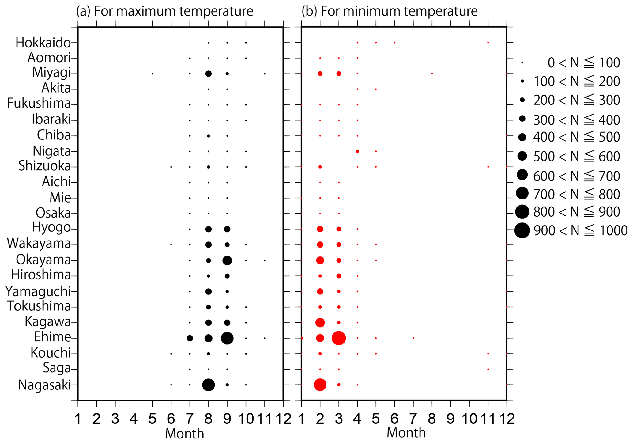
Figure 2Distributions of the monthly number of data points (N) for (a) maximum and (b) minimum temperatures collected in each prefecture from the 302 most reliable monitoring sites.
For the 302 sites, we evaluated whether the water temperature (Fig. 4a–b) and pHinsitu (Fig. 4c–d) were correlated at adjacent monitoring sites in the same prefecture (Fig. 4). At most of the stations, the correlations between the temperatures at the site pairs were relatively strong, which indicates that the temperature followed similar patterns over time at adjacent sites (Fig. 4a–b). The correlations tended to be strong when the sites were close together but gradually weakened with increasing distance between sites. The pHinsitu correlations followed a similar pattern (Fig. 4), which indicates that the pHinsitu and temperature data at adjacent monitoring sites varied in the same way. In other words, the relative ratios of the measurement errors in pHinsitu and the natural spatiotemporal variations at these monitoring sites were similar to those for temperature. The absolute values of the correlation coefficients for the pHinsitu were slightly lower than those for temperature for each corresponding pair of sites (Figs. 4 and 5) and might reflect the fact that pHinsitu but not the water temperature is subjected to strong forcing by coastal biological processes and other severe physical processes in summer, which causes the pHinsitu to vary in the short term. The correlations between the minimum pHinsitu data (Fig. 4c) were weaker than those for the maximum pHinsitu data (Fig. 4d) because the degree of biological forcing varied by season and was stronger in summer when the pHinsitu was at a minimum and weaker in the winter when the pHinsitu was at a maximum. Despite the influence of biological processes on the pHinsitu, the correlation coefficients remained high and were significant (r = 0.367, p<0.05) at most of the monitoring sites, especially at sites that were less than 5 km apart within the same prefecture, where the pHinsitu followed similar patterns. In the final step of the quality check procedure (step 3), we removed all the time sequences with weak and insignificant correlations for temperature and pHinsitu (Fig. 5) because we considered that the monitoring sites having both significant correlations for water temperature and pHinsituwere reliable. After this final step, 289 sites remained. As shown in Table 2, the correlations between temperature and pHinsitu at sites within 15 km of each other strengthened after steps 2 and 3, which suggests that the reliability of the dataset improved at each step of the quality control.
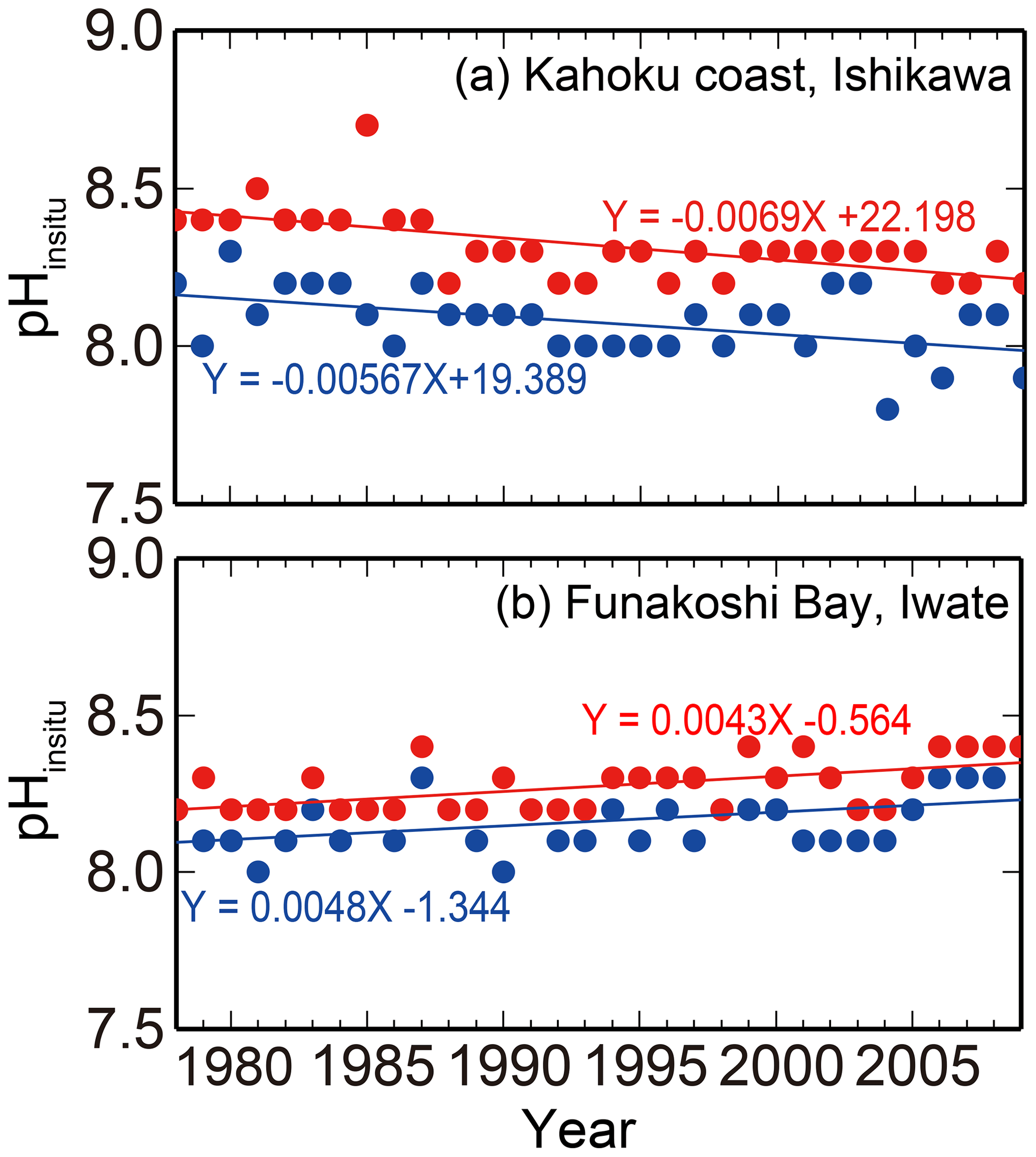
Figure 3Examples of (a) acidification (Kahoku coast in Ishikawa) and (b) basification (Funakoshi Bay in Iwate) trends at monitoring sites. Blue and red colors indicate the annual minimum and maximum pHinsitu data and their trends, respectively.
Table 2Average mutual correlation coefficients among water temperature and pHinsitu measurements at adjacent monitoring sites in the same prefecture. The averages were calculated from the data for the highest and lowest temperature, and minimum and maximum pHinsitu within 15 km for the three criteria. We refined the sites using three quality control steps, yielding 1481 (step 1), 1127 (step 2), and 302 (step 3) sites. The two rightmost columns represent a significant level of 5 % and a degree of freedom for the correlation coefficients of each quality check procedure.


Figure 4Correlations of water temperature and pHinsitu at adjacent monitoring sites in the same prefecture. Thin lines denote significant correlations (r=0.12, degrees of freedom = 283).
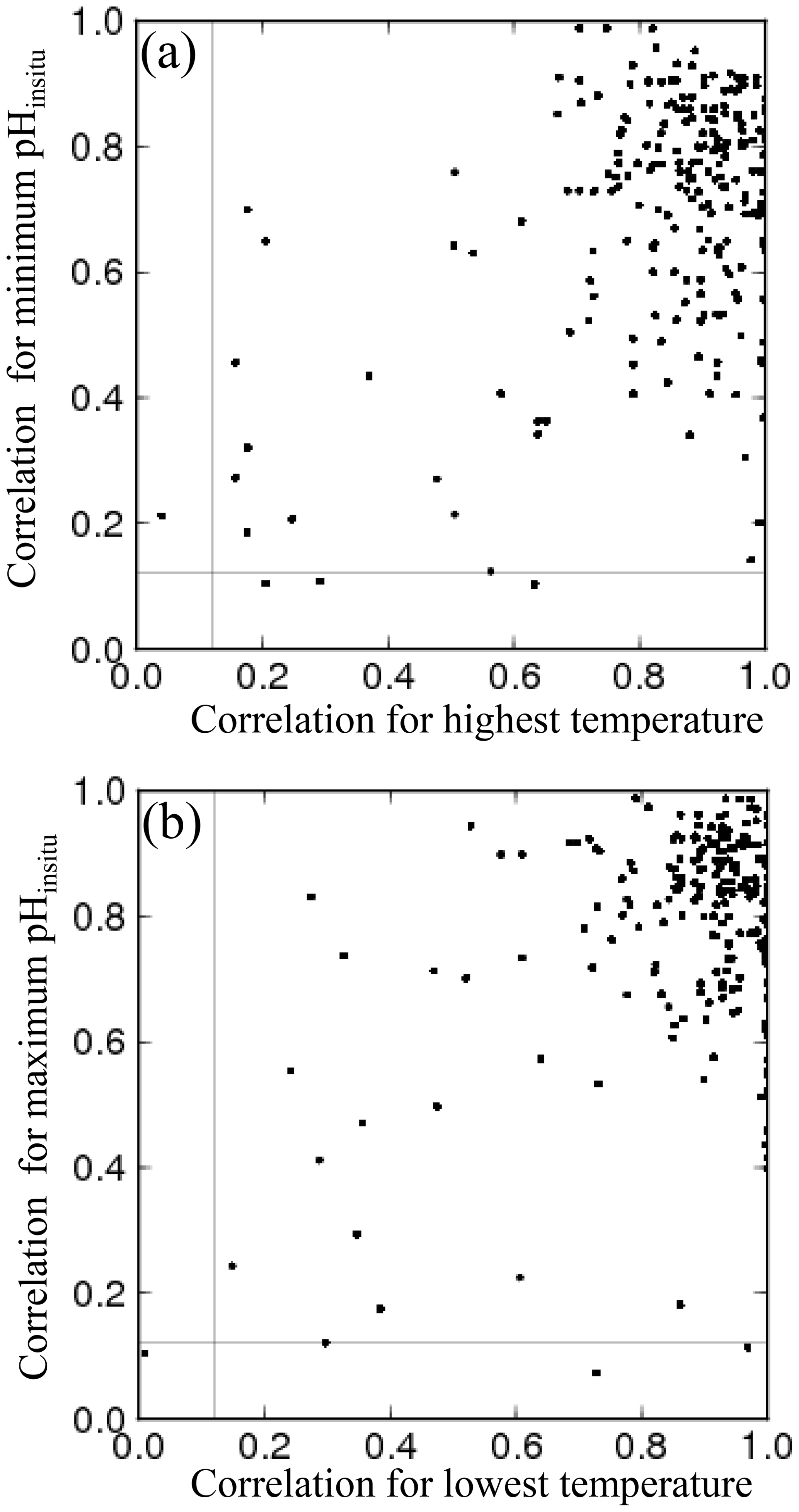
Figure 5Scatter plots of correlation coefficients for water temperature and pHinsitu at adjacent monitoring sites in the same prefecture. Panel (a) shows the highest temperature and the minimum pHinsitu, and panel (b) shows the lowest temperature and maximum pHinsitu.
The monitoring in each prefecture is carried out by different licensed operators, decided by the Regional Development Bureau in each prefecture. Intercalibration measurements have not been conducted between different licensed operators. Even though all the operators follow the same JIS protocol, manual monitoring can introduce systematic errors into the data. Some adjacent monitoring sites are close to each other but are managed by different operators, such as sites close to the boundaries between Osaka and Hyogo (Fig. 6a), Hyogo and Okayama (Fig. 6b), Kagawa and Okayama (not shown), and Kagawa and Ehime (not shown). The pHinsitu time sequences for these site pairs were generally similar, even though there were some deviations when compared with the time sequences for adjacent sites within the same prefecture, monitored by the same operator (lines of the same color in Fig. 6). The standard deviations of the pHinsitu trends between these site pairs close to the boundaries of Osaka and Hyogo, Hyogo and Okayama, Kagawa and Okayama, and Kagawa and Ehime were 0.0014, 0.0012, 0.0026, and 0.0017 yr−1, respectively, and were smaller than the acceptable measurement errors of the JIS standard protocols. We can therefore assume that the measurements from the different operators in different prefectures were consistent.
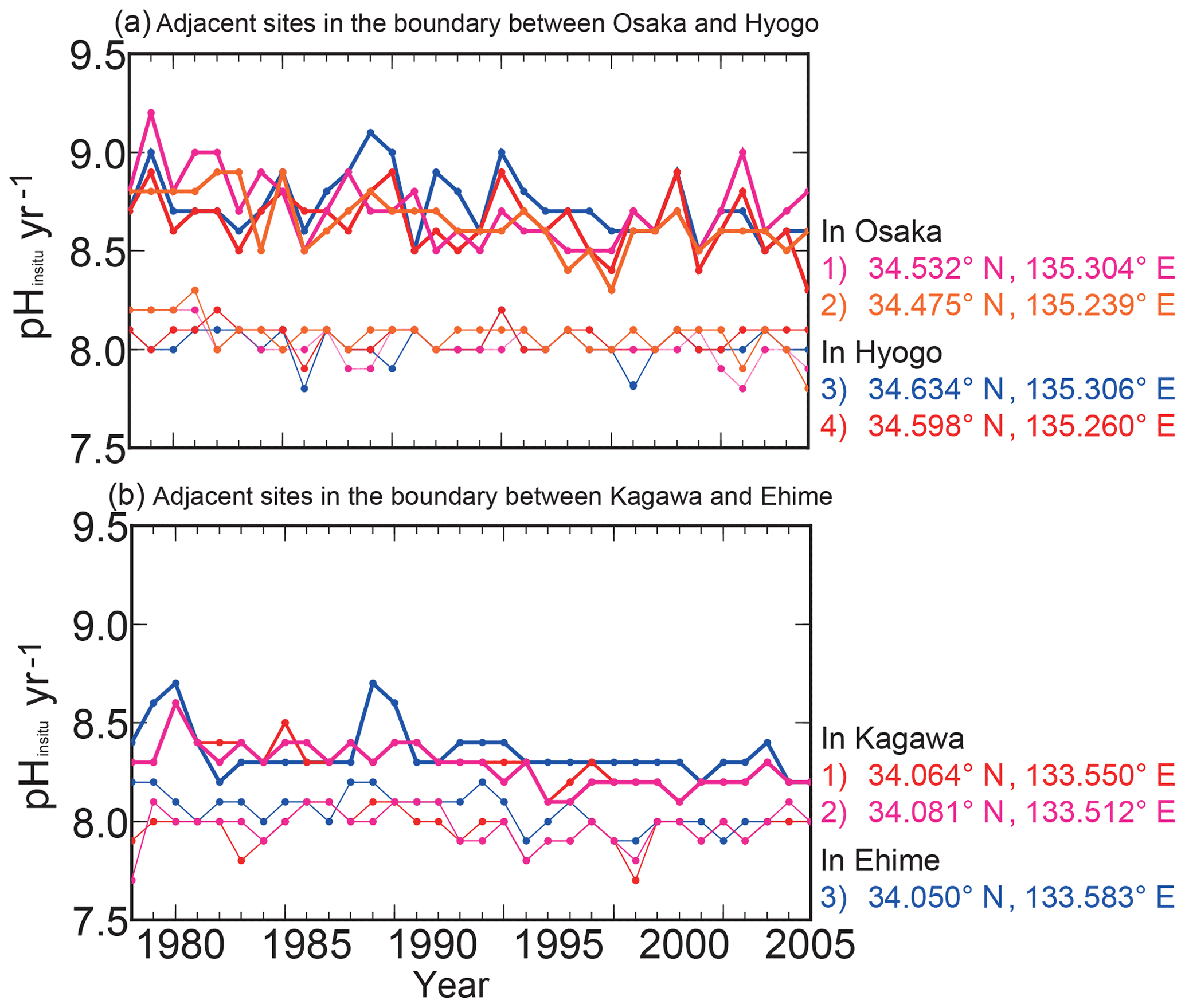
Figure 6Examples of time series for annual minimum and maximum pHinsitu data at adjacent monitoring sites close to the boundaries between (a) Osaka and Hyogo and (b) Kagawa and Ehime. Lines of the same color indicate data collected at the same site. Thin and bold lines indicate the annual minimum and maximum pHinsitu data, respectively, at each monitoring site. Site locations are included to the right of each panel, with the text color corresponding to the colors in each panel.
3.1 Variations in pHinsitu highlighted by regression analysis
The histograms of the calculated pHinsitu trends (yr−1) for the minimum and maximum pHinsitu after each quality control step are shown in Fig. 7. The histogram in Fig. 7a–b shows the data for the 1481 sites (discontinuous sites excluded). The data for the 1127 sites from step 2 (i.e., data without outliers) are shown in Fig. 7c–d, and the data for the 289 sites from step 3 are shown in Fig. 7e–f (Sect. 2.2). The number of sites decreased at each step of the quality control, but the shapes of the histograms were generally similar for both the minimum and maximum pH trends. The total trends showed overall normal distributions with a negative shift at all levels of quality control.
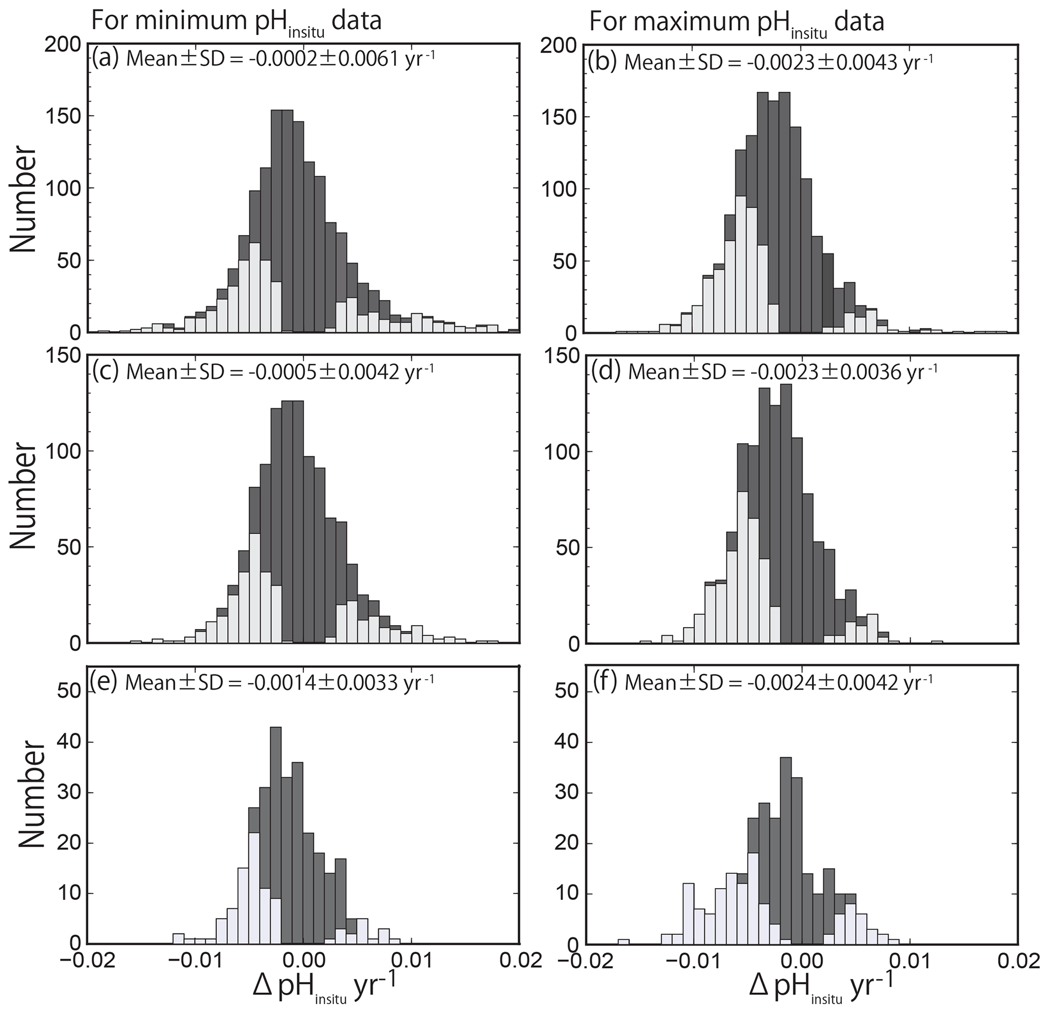
Figure 7Histogram of pH trends, represented by ΔpHinsitu, showing the slopes of the linear regression lines for the annual minimum (a, c, e) and maximum (b, d, f) pHinsitu data at each monitoring site. The histograms in (a, b), (c, d), and (e, f) show three scenarios: (a, b) all 1481 available sites with continuous records before quality control, (c, d) 1127 sites without outliers, and (e, f) 289 sites that meet the strictest criterion. The trends with statistical significance are denoted by light gray.
We detected both positive (basification) and negative (acidification) trends, which contrasts with the findings of other researchers who reported only negative trends (ocean acidification) in the open ocean (Bates et al., 2014; Midorikawa et al., 2010; Olafsson et al., 2009; Wakita et al., 2017). The average (± standard deviation) trends for the minimum and maximum pHinsitu data were and yr−1 for the 1481 sites (Fig. 7a–b) and and yr−1 for the 1127 sites (Fig. 7c–d), respectively. The average trends for the minimum and maximum pHinsitu data for the 289 sites that remained after step 3 were and yr−1, respectively (Fig. 7e–f).
The negative trends were relatively weak for the minimum pHinsitu data and relatively strong for the maximum pHinsitu data, but there was an overall tendency towards acidification. At the 289 sites, there were 204 negative and 86 positive trends for the minimum pHinsitu data and 217 negative and 72 positive trends for the maximum pHinsitu data. This shows that, for the minimum pHinsitu data, there were acidification and basification trends at 70 % and 30 % of the monitoring sites, respectively, and at 75 % and 25 % for the maximum pHinsitu data, respectively.
3.2 Local patterns in acidification and basification
We examined the pHinsitu trends for the 289 sites for local patterns in acidification and basification (Sect. 2.2) and found that the trends seemed to be randomly distributed. For example, the values were different at sites that were less than 50 km apart (Fig. 8). There are many monitoring sites in the Seto Inland Sea and in western Kyushu. The trends for the minimum and maximum pHinsitu showed both acidification and basification in the Seto Inland Sea (Fig. 8a–d). In the western part of Kyushu, acidification dominated (Fig. 8a–d) with only basification in pHinsitu at a few sites for both the minimum and maximum pHinsitu data (Fig. 8b, d). Figure 8a (Fig. 8b) and Fig. 8c (Fig. 8d) are similar, which suggests that, at most of the sites where we detected acidification and basification, the trend directions were consistent for the minimum and maximum pHinsitu (Fig. 8a–d).
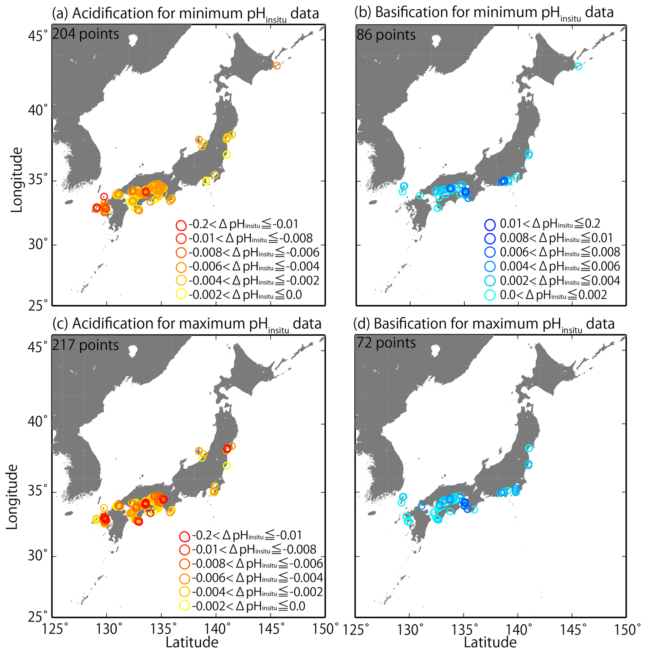
Figure 8Distributions of long-term trends in pHinsitu (ΔpHinsitu yr−1) in Japanese coastal seawater. The colors indicate the ranges of acidification (a, c) and basification (b, d). Panels (a, b) and (c, d) are linked to the data used in Fig. 7e and f, respectively.
By examining the average minimum and maximum pHinsitu trends in each prefecture (Fig. 9a–b, d–e, g–h, j–k), we found that, while the average values were slightly different, the trends in the averaged values and the patterns in acidification and basification for both the minimum and maximum pHinsitu were the same from north to south and from west to east. We also found acidification trends in most of the prefectures with at least 17 sampling sites, namely Miyagi, Wakayama, Hyogo, Okayama, Yamaguchi, Tokushima, Kagawa, Ehime, and Nagasaki (Figs. 1a and 9c, f, i, l). The average estimates for the maximum pHinsitu were larger than those for the minimum pHinsitu in these prefectures.

Figure 9(a, b, d, e, g, h) Average minimum and maximum pHinsitu trends (ΔpHinsitu yr−1) in each prefecture. These panels show each side of the Pacific Ocean (a, b), the Seto Inland Sea (d, e), the East China Sea (g, h), and the Sea of Japan (j, k). The prefecture names are arranged vertically from eastern (northern) to western (southern) areas. Black shading indicates a single standard deviation from the average. (c, f, i, l) Number of monitoring sites in each prefecture, and the thin dashed line is the threshold value of 17 (i.e., the average number of monitoring sites in all prefectures). The prefectures that meet the threshold are indicated in pink. This figure is based on the results shown in Figs. 7e and f and 8.
We found more acidification trends for the minimum pHinsitu in the southwestern prefectures of Yamaguchi, Kagawa, Ehime, Hyogo, and Nagasaki than in the northeastern prefecture of Miyagi (Fig. 9a, d, g, i) (see Fig. 1 for locations). The maximum and minimum pHinsitu trends indicated basification in Wakayama and Okayama prefectures (Fig. 9c). The trends in Osaka, Hyogo, Okayama, Hiroshima, Yamaguchi, Kagawa, and Ehime prefectures (Fig. 1a) were different, even though they were all located in the same part of the Seto Inland Sea (Fig. 9d–e). The trends in Hiroshima and Okayama, within the Seto Inland Sea, were weaker than those in Hyogo, Yamaguchi, Kagawa, and Ehime, which were outside the sea (Fig. 9d–e). The pHinsitu trend values indicated relatively strong acidification at a rate of −0.0025 yr−1 in Niigata in the Sea of Japan (Fig. 9j–l), but there were fewer than the threshold of 17 monitoring sites in the prefectures.
4.1 Statistical evaluation of our estimated overall trends
The JIS Z8802 (2011) allows a measurement error of ±0.07 and this treatment further enhanced the uncertainty of the published data to ±0.1. The uncertainty of the slope of the linear regression line (σβ) is estimated with the following equation (e.g., Luenberger, 1969):
where is the theoretical variance in a pH value caused by the measurement error (in this case, 0.12=0.01) and xi and [x] represent the year and the year averaged for all data at a station, respectively. In the WPCL dataset, there are generally 32 data points for each station (for every year from 1978 to 2009), spaced at consistent intervals. In this case, Σ(xi−[x])2 becomes 2728 and σβ becomes 0.0020 yr−1, which is the threshold of significance for the pH trend. This means that our estimated trends included standard deviations that were less than 0.0020 yr−1, and, if there were no trends, a histogram of the pH trends should be normally distributed with an average and standard deviation (σβ) of 0.0000 and 0.0020 yr−1, respectively (Fig. 7). The average trend in the maximum pHinsitu, however, shifted from zero in a negative direction at a rate of more than 0.0020 yr−1 for all three scenarios (Fig. 7b, d, f). This result implies that, averaged over the whole country, the Japanese coast was acidified in winter to a degree that could be detected from the historical WPCL pH data, even with an uncertainty of ±0.1. The observed standard deviation for the maximum pHinsitu was also larger than the expected value of 0.0020 yr−1 because of local variations in the pH trends. The average shift in the minimum pHinsitu data was smaller than 0.0020 yr−1, but all three scenarios showed negative shifts in the average minimum pHinsitu value (Fig. 7a, c, e).
We used Welch's t test to assess the direction of the average minimum and maximum pHinsitu trends. For our null hypothesis, we assumed that the population of the trends with an average of −0.0014 yr−1 (−0.0024 yr−1) and a standard deviation of 0.0033 yr−1 (0.0042 yr−1) was sampled from a population of the minimum (maximum) pHinsitu trends with an average trend of 0.0000 yr−1 and a standard deviation of 0.0020 yr−1. When the sample size was 289, the t values and the degrees of freedom were 8.7 (6.2) and 412.2 (474.4), respectively. Since the p value was less than 0.001, the null hypothesis was rejected. Welch's t test confirmed that the average trends for both the minimum and maximum pHinsitu data were negative.
We also applied a paired t test to determine whether the two trends calculated from the averaged minimum and maximum pHinsitu data were significantly different. The population mean and the sample size were 0.0 and 289, respectively. The t value of 4.64 (with 288 degrees of freedom) shows that the null hypothesis was rejected, with the paired t test thus indicating that the two trends calculated from the averaged minimum and maximum pHinsitu data were significantly different.
4.2 Effects of sampling depth
The WPCL dataset did not discriminate between surface (0.5–2 m) and subsurface (10 m) data when calculating the annual maximum and minimum pHinsitu, although monitoring depths were fixed throughout the monitoring period at all the sites. For temperature, the WPCL dataset provided data with the observed depth. Therefore, we estimated the percentage possibility that samples were collected at 10 m depth for the quality-controlled datasets with 1481, 1127, and 289 sites, assuming that pH values were measured at the same depth as temperature, and found that samples might have been collected at a depth of 10 m at 13 %, 13 %, and 15 % of the 1481, 1127, and 289 sites, respectively.
Usually the pH is lower in subsurface water than in surface water, as primary production decreases and increases the DIC concentrations in surface and subsurface water, respectively, because of decomposition when particulate organic carbon (POC) is produced by primary producers. We therefore speculate that the annual maximum pH includes very little data from a depth of 10 m, thus this value does represent the winter pH of surface waters. In contrast, the annual minimum pH was somewhat difficult to interpret, as it may have contained data from 10 m at some monitoring sites but only surface data at other sites shallower than 10 m.
Results of statistical analysis (Sect. 4.1) confirm that the trends in minimum and maximum pHinsitu data tended to be negative in the seawater around Japan. The negative tendency of the annual maximum pHinsitu trends may imply a trend of overall acidification in winter in surface waters around the Japanese coast, but the pattern in the annual minimum pHinsitu trends was difficult to interpret. Nevertheless, the annual minimum pHinsitu trends were, as for the annual maximum pHinsitu, also negative (Sect. 3.1), and the trends in the annual minimum pHinsitu and in the annual maximum pHinsitu showed similar patterns locally (Sect. 3.2), which indicate that long-term variations in the annual minimum and maximum pHinsitu were controlled by the same forcing, thus the pHinsitu trends changed in the same direction at both surface and subsurface. Global phenomena such as increases in atmospheric CO2 and warming of surface water temperatures may cause these forcings.
4.3 Possible influences on the pHinsitu trends in coastal seawater
To facilitate our discussion of the factors that influenced the pHinsitu trends further, we used the conceptual models of acidification and basification in coastal seawater of Sunda and Cai (2012) and Duarte et al. (2013), as follows:
The pHinsitu varies with the ambient temperature (T) on seasonal, inter-annual, and decadal timescales mainly because of changes in the dissociation constants of carbonate and bicarbonate (D(T)) in dissolved inorganic carbon (DIC), alkalinity (Alk), and salinity (S) also affect the pHinsitu trends. The solubility pump, which is controlled mainly by atmospheric CO2 concentration (AirCO2) and temperature, affects DIC, and ocean acidification occurs when the AirCO2 increases. Dissolved organic carbon can also be affected by biological processes (B) that depend on the ambient temperature (T) and the nutrient loading (N). There are contrasting relationships between DIC and N in heterotrophic and autotrophic waters. In the waters where organic decomposition is dominated by primary productivity (i.e., autotrophic water), increases in N will enhance primary production and cause DIC to decrease, raising pH (basification). When N increases in the waters adjoining this autotrophic water mass (for example, subsurface waters), POC transport from the autotrophic water mass will also increase, and DIC will increase as POC decomposes (i.e., heterotrophic water), causing acidification (e.g., Sunda and Cai, 2012; Duarte et al., 2013). In most coastal regions with low terrestrial input, water column productivity is mainly maintained by a one-dimensional nutrient cycle: primary production consumes nutrient and DIC to generate POC, and this POC sinks to subsurface and is then decomposed in subsurface water and/or seafloor to generate nutrients. As this result, in most coastal stations, surface water becomes autotrophic while subsurface water becomes heterotrophic. In estuary waters and waters near urbanized areas with high terrestrial input, however, decomposition of terrestrial POC often overcomes local primary production, and as a result, both surface and subsurface waters become heterotrophic (e.g., Kubo et al., 2017). If we assume that input of terrestrial POC varies in proportion to that of terrestrial N, we can expect that most of these stations show a heterotrophic response to N variation. Alkalinity (Alk) generally varies with salinity (S) in coastal oceans and may also affect the pHinsitu trend.
The DIC process (AirCO2) of ocean acidification shown in Eq. (2) generally occurred at all monitoring sites when the AirCO2 concentrations were horizontally uniform, resulting in overall negative trends in minimum and maximum pHinsitu. There was also an overall warming trend in D (T) in Japanese coastal areas, which may have affected the observed pHinsitu trend. Both the DIC (AirCO2) and D (T) may be associated with global processes of warming and ocean acidification, which were triggered by the increases in CO2 concentrations in the global atmosphere.
It is difficult to observe general trends in both DIC (B (T, N)) and Alk (S) at all monitoring sites because there were no common trends in the factors that control these variables (e.g., salinity of coastal water and terrestrial nutrient loadings) around the Japanese coast in this dataset. The WPCL data contain stations with both autotrophic surface water and heterotrophic subsurface waters, which further obscures the influence of DIC (B (T, N)) on the overall pHinsitu trend, as the same trend in B (T, N) leads to opposite trends in DIC (B (T, N) in autotrophic and heterotrophic waters (Duarte et al., 2013). The wide variations in DIC (B (T, N)) and Alk (S) between regions might have caused the regional differences in pHinsitu trends among stations, contributing to relatively large standard deviations in both the minimum and maximum pHinsitu trends (Fig. 7). The three-step quality control procedures effectively removed the sites with high variability due to analytical errors, and this process may also have removed the effect of large local processes (e.g., heavy phytoplankton bloom or freshwater discharge change). Nevertheless, we still are able to detect regional-scale difference in the distribution of positive and negative trends (e.g., Fig. 8). Therefore, we discuss the effects of global processes on the overall average pH trends and of regional effects separately in later sections (Sect. 4.3.1 and 4.3.2).

Figure 10Same as Fig. 7 but showing the pH25 trends at 289 sites (selected by quality control step 3). The value of pH25 was estimated using the method of Lui and Chen (2017).
4.3.1 Global effects on pHinsitu trends
Our analysis was based on pHinsitu data, so differences observed in trends may reflect long-term changes in water temperature that affected the dissociation constant (process D (T) in Eq. 2) or changes in the coastal carbon cycle, including absorption of anthropogenic carbon by the solubility pump (process DIC (AirCO2) in Eq. 2). Some of the effects of D (T) and DIC (AirCO2) driven by global warming and ocean acidification may have affected all monitoring sites and may have contributed to the negative shifts in trend distributions.
To evaluate the direct thermal effects related to process D (T) in Eq. (2), we estimated the pH values normalized to 25 ∘C (pH25), assuming that the minimum (maximum) pHinsitu and highest (lowest) temperature and other parameters were measured at the same time. By assuming the other parameters that affected the pH calculation in the CO2sys (Lewis and Wallace 1998, csys.m), such as salinity, DIC, and alkalinity, did not change (these parameters are not measured as part of the WPCL program), we used the method of Lui and Chen (2017) to calculate the pH25, as follows:
where a1 was set to −0.015 and T was the observed temperature.
The distributions of the trends in pH25 after applying Eq. (3) are shown in Fig. 10. The minimum and maximum pH25 data were normally distributed, meaning that the distributions of the pHinsitu trends were maintained after applying Eq. (3) (Fig. 7e, f). The averages (± standard deviations) of the minimum and maximum pH25 trends were and yr−1, respectively. The averaged trends are consistent with those reported by Midorikawa et al. (2010), who calculated that the pH25 decreased at rates of and yr−1 in summer and winter from 1983 to 2007 along the 137∘ E line of longitude in the North Pacific. The asymmetry of pH25 trends between the minimum and maximum estimates may be related to seasonal variations in pCO2 and associated asymmetric responses of the air–sea CO2 flux (Landschutzer et al., 2018; Fassbender et al., 2018).
We used Welch's t test to assess the direction of the averages of minimum and maximum pH25 trends. The p value was less than 0.001, so the null hypothesis was rejected again. The results of the t test confirm that the average trends for both the minimum and maximum pH25 data were also negative, suggesting that the DIC (AirCO2) effect (i.e., ocean acidification) caused the negative shifts in the distribution of the trend for the pH normalized to 25 ∘C.
The pH25 and pHinsitu trends from north to south and from west to east were similar among the prefectures (Fig. 11), except in Miyagi and Tokushima. The trends in the minimum pHinsitu and summer pH25 were quite similar, but the minimum and maximum pHinsitu trends tended to be more negative (by about −0.0010 yr−1) than the corresponding pH25 trends, especially in Wakayama, Hiroshima, Kagawa, and Ehime, which met the threshold number of sampling sites.
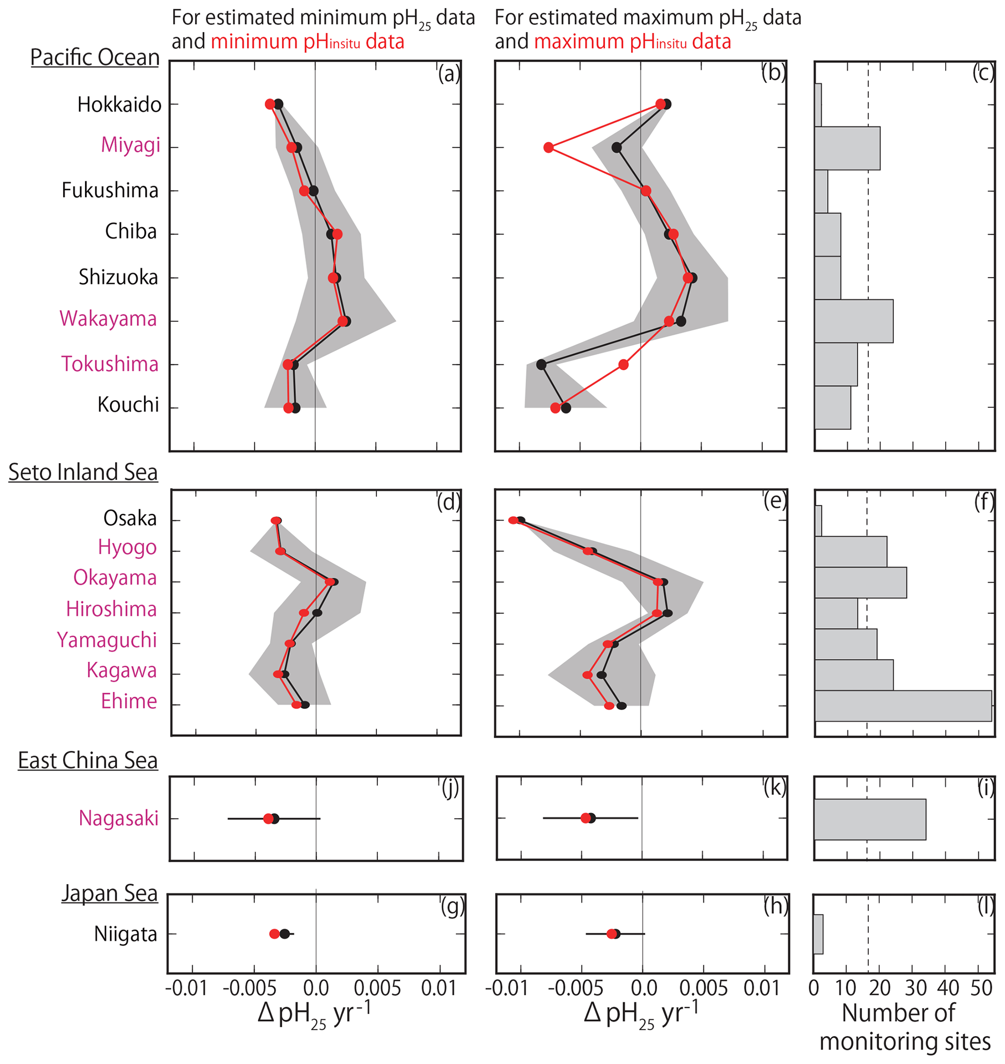
Figure 11(a, b, d, e, g, h, j, k) Same as Fig. 9 but showing the average estimated minimum and maximum pH25 trends (ΔpH25 yr−1) for each prefecture. Red lines and points indicate the average minimum and maximum pHinsitu trends shown in Fig. 9.
The average highest temperatures observed at the minimum pHinsitu were close to 25 ∘C in the regions south of Chiba prefecture (Figs. 1 and 12a–d), so the normalization at 25 ∘C did not have much effect on the minimum pH25 in the southern prefectures. In contrast, the maximum pHinsitu values were observed at temperatures that were more than 10 ∘C lower than 25 ∘C, so the normalization worked well on the winter data. We estimated the temperature trends from the highest and lowest temperatures at the 289 sites that remained after quality control step 3. The trends in the highest and lowest temperatures generally indicated warming, with an average and standard deviation of 0.021±0.040 and 0.047±0.036 ∘C yr−1, respectively (Fig. 13). Estimations from the CO2sys indicate that these warming trends influenced the pH values and were related to the changes of −0.0004 and −0.0010 yr−1 in the pH trends in summer and winter, respectively (Figs. 7e–f and 10a–b).
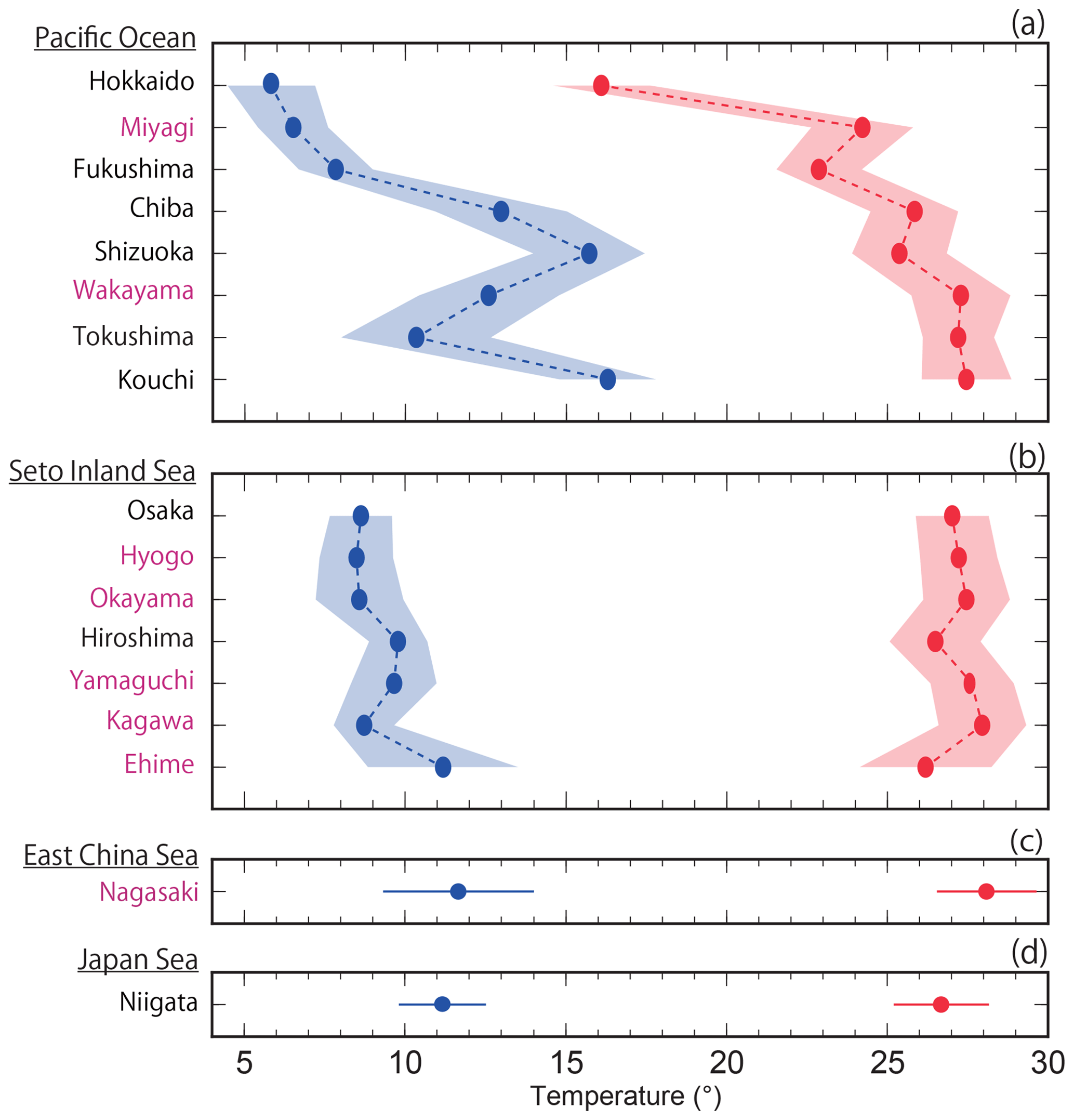
Figure 12Average highest and lowest temperatures observed for the minimum and maximum pHinsitu data for each prefecture. The blue and red lines and shading indicate the average and one standard deviation from the average, respectively. The prefectures that met the threshold of 17 are shown in purple, as in Figs. 9c–l and 11c–l.
We estimated thermal effects and that the pHinsitu would change from 8.0150 to 8.0147 in summer and from 8.2568 to 8.2560 in winter, for temperature changes from 25.00 to 25.02 ∘C, and from 10.00 to 10.04 ∘C, respectively, for a salinity of 34, DIC of 1900 mmol m−3, and alkalinity of 2200 mmol m−3. The differences between the pHinsitu and the corresponding pH25 trends in summer (−0.0004 yr−1) and winter (−0.0010 yr−1) can be partly explained by the difference between the decrease in the pH trends in summer (−0.0003 yr−1) and winter (−0.0008 yr−1) arising from the thermal effects.
4.3.2 Local effects on pHinsitu trends
We found regional differences in the pHinsitu values (e.g., Figs. 6) and pHinsitu trends (Figs. 8–9). The negative pHinsitu trends (acidification) were more significant in southwestern Japan than in northeastern Japan, especially for the minimum pHinsitu data (Fig. 9 and Sect. 3.2). The Japanese Meteorological Agency (2008, 2018) reported that, over the past 100 years, the increase in water temperature in western Japan was ∼1.30 ∘C greater than that in northeastern Japan.
We used CO2sys (Lewis and Wallace, 1998) to predict how pHinsitu would change under a temperature difference of 0.01 ∘C yr−1 between the northeastern and southwestern areas, and found that pH decreased by 0.0002 (0.0002) yr−1 when the temperature changed from 10.00 to 10.01 ∘C (25.0 to 25.01 ∘C), assuming a salinity of 34, DIC of 1900 mmol m−3, and alkalinity of 2200 mmol m−3. The contrasting trends in the northeast and southwest can also be partly explained by the difference in warming trends (process D (T) in Eq. 2).
The summer pHinsitu is affected by ocean uptake of CO2 (process DIC in Eq. 2; Bates et al., 2012; Bates, 2014) through long-term changes in biological activity (Cai et al., 2011; Sunda and Cai, 2012; Duarte et al., 2013; Yamamoto-Kawai et al., 2015), as well as the effect of changes in the dissociation constant. The responses of pHinsitu to changes in marine productivity are, however, complicated.
Previous studies have reported that nutrient loadings in Japan have decreased over recent decades (e.g., Yamamoto-Kawai et al., 2015; Kamohara et al., 2018; Nakai et al., 2018), with variable effects on summer pHinsitu in coastal seawater. TN was monitored for a shorter period than pHinsitu (1995 to 2009). We assumed that the TN was mainly dissolved inorganic nitrogen and determined the correlations between TN and the minimum and maximum pHinsitu trends (Fig. 14). There were statistically significant negative correlations between TN and the minimum (−0.30) and maximum (−0.29) pHinsitu trends. Such negative correlation was actually produced by existence of low ΔTN and low ΔpH cluster (eight stations, highlighted by dotted blue circles in Fig. 14). We recognized that the all sites were measured in the same bay, Shimotsu Bay, Wakayama Prefecture. The bay seemed to change the volume of the terrestrial nutrient input during the monitoring period and decreased its TN input, resulting in significant basification in the water.

Figure 13Same as Fig. 7 but showing the highest and lowest temperature trends at 289 sites (selected by quality control step 3).
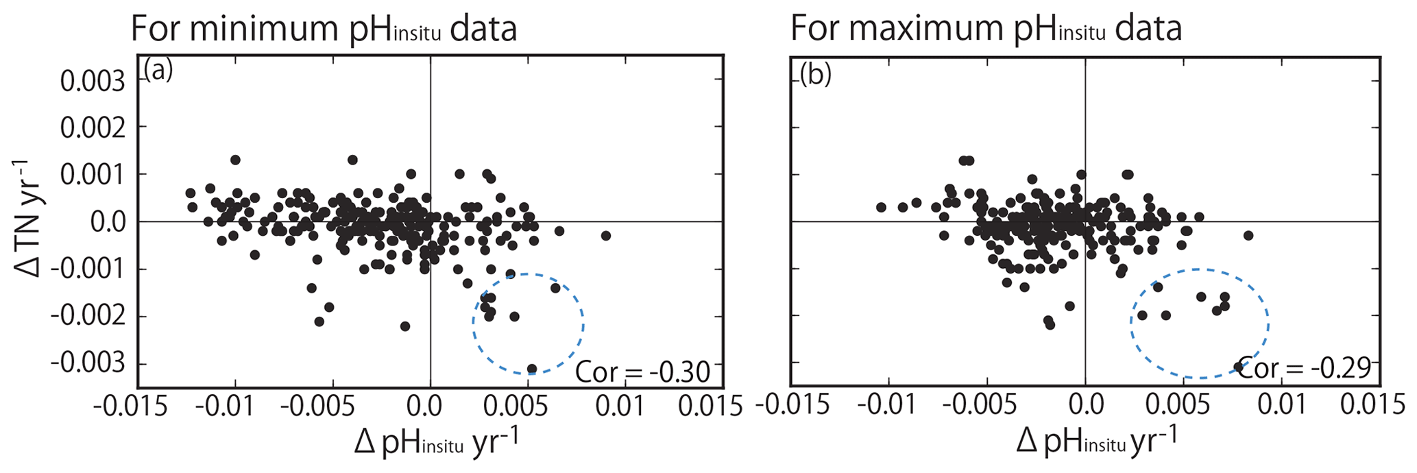
Figure 14Correlation between trends in total nitrogen (TN) and trends in (a) minimum and (b) maximum pHinsitu. The correlation coefficients are −0.30 and −0.29 for the minimum and maximum pHinsitu, respectively (significance level of 0.05, r= 0.128; degrees of freedom = 236). Dotted blue circles indicate the data measured in Shimotsu Bay in Wakayama Prefecture.
For other stations, however, acidification and basification processes seem to occur independently to the changes in TN input. The pH can change even with a constant primary production rate if a residence time of coastal water changes (for the case of autotrophic water, a shorter residence time could cause lower pH). Some parts of stations with significant basification and small ΔTN may have experienced such changes in the water residence time (e.g., artificial changes in the closure rate of the inlet, although we have no hydrography data directly proving this assumption at the present time.
Nakai et al. (2018) reported that nutrient loadings decreased in the most parts of the Seto Inland Sea from 1981 to 2010 but that several areas remained eutrophic. Because of geographical variations in nutrient loadings and the uneven distribution of autotrophic and heterotrophic stations, there are significant spatial variations in pH trends in the Seto Inland Sea (Fig. 8). The pH trends in coastal areas of western Kyushu, where the anthropogenic nutrient loadings are relatively low, therefore reflect the decreases in nutrient discharges, resulting in variations between regions (e.g., Nakai et al., 2018; Yamamoto and Hanazato, 2015; Tsuchiya et al., 2018). Several cities in this area have introduced advanced sewage treatment to prevent eutrophication in coastal seawater (Nakai et al., 2018; Yamamoto and Hanazato, 2015).
Regional variations in coastal alkalinity, along with salinity, might be related to changes in land use and might affect these trends (process Alk(S) in Eq. 2). Taguchi et al. (2009) measured alkalinity in the surface waters of the Ise, Tokyo, and Osaka bays between 2007 and 2009 and reported that total alkalinity was highly correlated with salinity in each bay. For a temperature, salinity, inorganic dissolved carbon, and total alkalinity of 25 ∘C, 35, 1900 and 2300 mmol m−3, respectively, pHinsitu (= pH25) was estimated at 8.1416 using the CO2sys (Lewis and Wallace, 1998). By changing the salinity and alkalinity to 34 and 2200 mmol m−3, respectively, pHinsitu (= pH25) decreased by 0.0081 to 8.0150. This shows that the pH could deviate significantly from average trends if the inputs of alkaline compounds are changed; consequently, some of our pH trends could have been affected by changing discharge from different land-use types.
Regional differences in pHinsitu trends in coastal seawater might be caused by ocean pollution. The speciation and bioavailability of heavy metals change in acidic waters, causing an increase in the bio-toxicity of the metals (Zeng et al., 2015; Lacoue-Labarthe et al., 2009; Pascal et al., 2010; Campbell et al., 2014). The rates at which marine organisms photosynthesize and respire in ocean waters decrease and increase, respectively, in water polluted with heavy metals and oils (process DIC in Eq. 2) because of bio-toxicity and eutrophication, thereby resulting in acidification (Hing et al., 2011; Huang et al., 2011; Gilde and Pinckney 2012).
We estimated the long-term trends in pHinsitu in Japanese coastal seawater and examined how the trends varied regionally. The long-term pHinsitu data show highly variable trends, although ocean acidification has generally intensified in Japanese coastal seawater. We found that the annual maximum pHinsitu at each station, which generally represents the pH of surface waters in winter, had decreased at 75 % of the sites and had increased at the remaining 25 % of sites. The temporal trend in the annual minimum pHinsitu, which generally represents the summer pH in subsurface water at each site, was also similar, but it was relatively difficult to interpret the trends of annual minimum pHinsitu because the sampling depths differed between stations. The average rate of decrease in the annual maximum pHinsitu was −0.0024 yr−1, with relatively large deviations from the average value. Detailed analysis suggests that the decrease in the pH was partly caused by warming of Japanese surface coastal seawater in winter. However, the distributions of the trend in pH normalized to 25 ∘C also showed negative shifts, suggesting that anthropogenic DIC was also increasing in Japanese coastal seawater.
There were striking spatial variations in the pHinsitu trends. Correlations among the pHinsitu time series at different sites revealed that the high variability in the pHinsitu trends was not caused by analytical errors in the data but reflected the large spatial variability in the physical and chemical characteristics of coastal environments, such as water temperature, nutrient loadings, and autotrophic and heterotrophic conditions. While there was a general tendency towards coastal acidification, there were positive trends in pHinsitu at 25 %–30 % of the monitoring sites, indicating basification, which suggests that the coastal environment might not be completely devastated by acidification. If we can manage the coastal environment effectively (e.g., control nutrient loadings and autotrophic and heterotrophic conditions), we might be able to limit, or even reverse, acidification in coastal areas.
Data are available in an institutional repository that does not issue datasets with DOIs (non-mandated deposition). The pH in situ data and information from monitoring sites are included in the Supplement. All data included in this study are available upon request via contact with the corresponding author.
The supplement related to this article is available online at: https://doi.org/10.5194/bg-16-4747-2019-supplement.
Conceptulization, TT; Methodology, MI, YM, and TO; Validation, MI; Formal analysis, MI; Writing-Original Draft Preparation, MI, YM, TO; Writing-Review and Editing, MI, YM, and TO; Visualization, MI; Supervision, YM and TO; Project administration, TT and YM; Funding Acquisition, TT and YM.
The authors declare that they have no conflict of interest.
We thank the scientists, captain, officers, and personnel of the National Institute for Environmental Studies, Regional Development Bureau of the Ministry of Land, Infrastructure, Transport, and Tourism, who contributed to this study. We acknowledge financial support from the Sasakawa Peace Foundation of the Ocean Policy Research Institute. We also appreciate discussions with members of the Environmental Variability Prediction and Application Research Group of the Japanese Agency for Marine-Earth Science and Technology. Suggestions by two reviewers helped us to improve an earlier version of the paper.
This research has been supported by the Sasakawa Peace Foundation of the Ocean Policy Research Institute (OPRI-SPF).
This paper was edited by Jean-Pierre Gattuso and reviewed by Abed El Rahman Hassoun and one anonymous referee.
Bates, N. R.: Interannual variability of the ocean CO2 sink in the subtropical gyre of the North Atlantic Ocean over the last 2 decades, J. Geophys. Res. 112, C09013, https://doi.org/10.1029/2006JC003759, 2007.
Bates, N. R., Astor, Y. M., Church, M. J., Currie, K., Dore, J. E., Gonzalez-Davila, M., Lorenzoni, L., Muller-Karger, F., Olafsson, J., and Santana-Casiano, J. M.: A time-series view of changing surface ocean chemistry due to ocean uptake of anthropogenic CO2 and ocean acidification, Oceanography, 27, 126–141, https://doi.org/10.5670/oceanog.2014.16, 2014.
Borges, A. V. and Gypen, N.: Carbonate chemistry in the coastal zone responds more strongly to eutrophication than to ocean acidification, Limnol. Oceanogr., 55, 346–353, 2010.
Byrne, M., Lamare, M., Winter, D., Dworjanyn, S. A., and Uthicke, S.: The stunting effect of a high CO2 ocean on calcification and development in the urchin larvae, a synthesis from the tropics to the poles, Philos. T. R. Soc. B, 368, 20120439, https://doi.org/10.1098/rstb.2012.0439, 2013.
Cai, W., Hu, X., Huang, W., Murell, M. C., Lehrter, J. C., Lohrenz, S. E., Chou, W., Zhai, W., Hollibaugh, J. T., Wang, Y., Zhao, P., Guo, X., Gundersen, K., Dai, M., and Gong, G.: Acidification of subsurface coastal waters enhanced by eutrophication, Nat. Geosci., 4, 766–700, 2011.
Campbell, A. L., Mangan, S., Ellis, R. P., and Lewis, C.: Ocean acidification increases copper toxicity to the early life history stages of the polychaete arenicola marina in artificial seawater, Environ. Sci. Technol., 48, 9745–9753, 2014.
Challener, R. C., Robbins, L. L., and McClintock, J. B.: Variability of the carbonate chemistry in a shallow, seagrass-dominated ecosystem: imprications for ocean acidification experiments, Mar. Fresh. Res., 67, 163–172, https://doi.org/10.1071/MF14219, 2016.
DOE (United States Department of Energy): Handbook of methods for the analysis of the various parameters of the carbon dioxide system in sea water, ver. 2, edited by: Dickson, A. G. and Goyet, C., ORNL/CDIAC-74, 1994.
Dore, J. E., Lukus, R., Sadler, D. W., Church, M. J., and Karl. D. M.: Physical and biogeochemical modulation of ocean acidification in the central North Pacific, P. Natl. Acad. Sci. USA, 106, 12235–12240, 2009.
Duarte, C. M., Hendriks, I. E., Moore, T. S., Olsen, Y. S., Steckbauer, A., Ramajo, L., Carstensen, J., Trotter, J. A., and McCullouch, M.: Is ocean acidification an open ocean syndrome? Understanding anthropogenic impacts in seawater pH, Estuar. Coast., 36, 221–236, https://doi.org/10.1007/s12237-013-9594-3, 2013.
Fassbender J. A., Rodgers B. K., Palevsky I. H., and Sabine L. C.: Seasonal asymmetry in the evolution of surface ocean pCO2 and pH thermodynamic drivers and the influence on sea-air CO2 flux, Global Biogeochem. Cy., 32, 11476–1497, 2018.
Frankignoulle, M. and Bouquegneau, J. M.: Daily and yearly variations of total inorganic carbon in a productive coastal area, Estuarine, Coast. Shelf Sci., 30, 79–89, 1990.
Gilde, K. and Pinckney, J. L.: Sublethal effects of crude oil on the community structure of estuarine phytokton, Estuar. Coast., 35, 853–861, 2012.
Gonzalez-Davila, M., Santana-Casiano, J. M., and Gonzalez-Davila, E. F.: Interannual variability of the upper ocean carbon cycle in the northeast Atlantic Ocean, Geophys. Res. Lett. 34, L07608, https://doi.org/10.1029/2006GL028145, 2007.
Hagens, M., Slomp, C. P., Meysman, F. J. R., Seitaj, D., Harlay, J., Borges, A. V., and Middelburg, J. J.: Biogeochemical processes and buffering capacity concurrently affect acidification in a seasonally hypoxic coastal marine basin, Biogeoscience, 12, 1561–1583, https://doi.org/10.5194/bg-12-1561-2015, 2015.
Hing, L. S., Ford, T., Finch, P., Crane, M., and Morritt, D.: Laboratory stimulation of oil-spill effects on marine phytoplankton, Aquat. Toxicol., 103, 32–37, 2011.
Huang, Y. J., Jiang, Z. G., Zeng, J. N., Chen, Q. Z., Zhao, Y. Q., Liao, Y. B., Shou, L., and Xu, X. Q.: The chronic effects of oil pollution on marine phytoplankton in a subtropical bay, China, Environ. Monit. Assess., 176, 517–530, 2011.
Japanese Industrial Standard Z8802: Methods for determination of pH of aqueous solutions, available at: http://kikakurui.com/z8/Z8802-2011-01.html (last access: 5 December 2019), 2011 (in Japanese).
Japanese Meteorological Agency (JMA): Global warming projections 7th, available at: http://dl.ndl.go.jp/view/download/digidepo_3011050_po_synthesis.pdf?itemId=_info%3Andljp%2Fpid%2F3011050&contentNo=_1&alternativeNo=_&_lang=_en (last access: 5 December 2019), 2008.
Japanese Meteorological Agency (JMA): Long-term trends of ocean surface temperature around the Japanese coast, available at: https://www.data.jma.go.jp/kaiyou/data/shindan/a_1/japan_warm/japan_warm.html, 2018 (in Japanese).
Kamohara, S., Takasu, Y., Yuguchi, M., Mima, N., and Yoshunari, A.: Nutrient decrease in Mikawa Bay, Bulletin of Aichi Fisheries Research Institute, 23, 30–32, 2018 (in Japanese).
Kubo, A., Maeda, Y., and Kanda, J.: A significant net sink for CO2 in Tokyo Bay, Nat. Sci. Rep., 7, 44345, https://doi.org/10.1038/srep44355, 2017.
Lacoue-Labarthe, T., Martin, S., Oberhänsli, F., Teyssié, J.-L., Markich, S., Jeffree, R., and Bustamante, P.: Effects of increased pCO2 and temperature on trace element (Ag, Cd and Zn) bioaccumulation in the eggs of the common cuttlefish, Sepia officinalis, Biogeosciences, 6, 2561–2573, https://doi.org/10.5194/bg-6-2561-2009, 2009.
Landschutzer, P., Gruber, N., Bakker, C. E. D., Stemmler, I., and Six, D. K.: Strengthening seasonal marine CO2 variations due to increasing atmospheric CO2, Nat. Clim. Change, 8, 146–150, 2018.
Lewis, E. and Wallace, D. W. R.: Program Developed for CO2 System Calculations. ORNL/CDIAC-105, Carbon Dioxide Information Analysis Center, Oak Ridge National Laboratory, US Department of Energy, Oak Ridge, Tennessee, 21 pp., 1998.
Luenberger, D. G.: Optimization by vector space methods, John Wiley & Sons, Inc., New York, NY, 1–326, 1969.
Lui, H. and Chen, A. C.: Reconciliation of pH25 and pHinsitu acidification rates of the surface oceans: A simple conversion using only in situ temperature, Limnol. Oceanogr.-Method., 15, 328–355, 2017.
Midorikawa, T., Ishii, M., Sailto, S., Sasano, D., Kosugi, N., Motoi, T., Kamiya, H., Nakadate, A., Nemoto, K., and Inoue, H.: Decreasing pH trend estimated from 25-yr time series of carbonate parameters in the western North Pacific, Tellus B, 62, 649–659, https://doi.org/10.111/j.1600-0889.2010.00474.x, 2010.
Millero, F. (Ed.): Chemical Oceanography, 4th Edn., CRC Press, New York, United States, 592 pp., 2013.
Ministry of the Environment: Methods of water quality survey, available at: http://www.env.go.jp/hourei/05/000140.html (last access: 5 December 2019), 2018 (in Japanese).
Nakai, S., Soga, Y., Sekito, S., Umehara, S., Okuda, T., Ohno, M., Nishijima, W., and Asaoka, S.: Historical changes in primary production in the Seto Inland Sea, Japan, after implementing regulations to control the pollutant loads, Water Policy, 20, 855–870, https://doi.org/10.2166/wp.2018093, 2018.
NIES (National Institute for Environmental Studies): Explanation of Water Pollution Control Law (WPCL) monitoring data, available at: https://www.nies.go.jp/igreen/explain/water/content_w.html (last access: 5 December 2019), 2018 (in Japanese).
Olafsson, J., Olafsdottir, S. R., Benoit-Cattin, A., Danielsen, M., Arnarson, T. S., and Takahashi, T.: Rate of Iceland Sea acidification from time series measurements, Biogeosciences, 6, 2661–2668, https://doi.org/10.5194/bg-6-2661-2009, 2009.
Pascal, P. Y., Fleeger, J. W., Galvez, F., and Carman, K. R.: The toxicological interaction between ocean acidity and metals in coastal meiobenthic copepods, Mar. Pollut. Bull., 60, 2201–2208, 2010.
Sunda, W. G. and Cai, W. J.: Eutrophication induced CO2-acidification of subsurface coastal waters: interactive effects of temperature, salinity, and atmospheric pCO2, Environ. Sci. Technol., 46, 10651–10659, 2012.
Taguchi, F., Fujiwara, T., Yamada, Y., Fujita, K., and Sugiyama, M.: Alkalinity in coastal seas around Japan, Bull. Coast. Oceanogr., 47, 71–75, 2009.
Tsuchiya, K., Ehara, M., Yasunaga, Y., Nakagawa, Y., Hirahara, M., Kishi, M., Mizubayashi, K., Kuwahara, V. S., and Toda, T.: Seasonal and Spatial Variation of Nutrients in the Coastal Waters of the Northern Goto Islands, Japan, Bull. Coast. Oceanogr., 55, 125–138, 2018 (in Japanese).
Wakita, M., Nagano, A., Fujiki, T., and Watanabe, S.: Slow acidification of the winter mixed layer in the subarctic western North Pacific, J. Geophys. Res.-Ocean., 122, 6923–6935, https://doi.org/10.1002/2017JC013002, 2017.
Waldbusser, G. G., Voigt, E. P., Bergschneider, H., Green, M. A., and Newell, R. I.: Biocalcification in the eastern oyster (Cassostrea virgnica) in relation to long-term terns in Chesapeak Bay pH, Estuar. Coast., 34, 221–231, 2011.
Yamamoto, T. and Hanazato, T.: Eutrophication problems of oceans and lakes – fishes cannot live in clean water, ChijinShokan Co. Ltd, ISBN978-4-8052-0885-4, 1–208, 2015 (in Japanese).
Yamamoto-Kawai, M., Kawamura, N., Ono, T., Kosugi, N., Kubo, A., Ishii, M., and Kanda, J.: Calcium carbonate saturation and ocean acidification in Tokyo Bay, Japan, J. Oceanogr., 71, 427–439, https://doi.org/10.1007/s10872-015-0302-8, 2015.
Zeng, X., Chen, X., and Zhuang, J.: The positive relationship between ocean acidification and pollution, Mar. Poll. Bull, 91, 14–21, 2015.