the Creative Commons Attribution 4.0 License.
the Creative Commons Attribution 4.0 License.
 | 25 Jan 2019
Sedimentary alkalinity generation and long-term alkalinity development in the Baltic Sea
Xiaole Sun
Daniel C. Reed
Christoph Humborg
Caroline P. Slomp
Bo G. Gustafsson
Enhanced release of alkalinity from the seafloor, principally driven by anaerobic degradation of organic matter under low-oxygen conditions and associated secondary redox reactions, can increase the carbon dioxide (CO2) buffering capacity of seawater and therefore oceanic CO2 uptake. The Baltic Sea has undergone severe changes in oxygenation state and total alkalinity (TA) over the past decades. The link between these concurrent changes has not yet been investigated in detail. A recent system-wide TA budget constructed for the past 50 years using BALTSEM, a coupled physical–biogeochemical model for the whole Baltic Sea area revealed an unknown TA source. Here we use BALTSEM in combination with observational data and one-dimensional reactive-transport modeling of sedimentary processes in the Fårö Deep, a deep Baltic Sea basin, to test whether sulfate () reduction coupled to iron (Fe) sulfide burial can explain the missing TA source in the Baltic Proper. We calculated that this burial can account for up to 26 % of the missing source in this basin, with the remaining TA possibly originating from unknown river inputs or submarine groundwater discharge. We also show that temporal variability in the input of Fe to the sediments since the 1970s drives changes in sulfur (S) burial in the Fårö Deep, suggesting that Fe availability is the ultimate limiting factor for TA generation under anoxic conditions. The implementation of projected climate change and two nutrient load scenarios for the 21st century in BALTSEM shows that reducing nutrient loads will improve deep water oxygen conditions, but at the expense of lower surface water TA concentrations, CO2 buffering capacities and faster acidification. When these changes additionally lead to a decrease in Fe inputs to the sediment of the deep basins, anaerobic TA generation will be reduced even further, thus exacerbating acidification. This work highlights that Fe dynamics plays a key role in the release of TA from sediments where Fe sulfide formation is limited by Fe availability, as exemplified by the Baltic Sea. Moreover, it demonstrates that burial of Fe sulfides should be included in TA budgets of low-oxygen basins.
Please read the corrigendum first before continuing.
-
Notice on corrigendum
The requested paper has a corresponding corrigendum published. Please read the corrigendum first before downloading the article.
-
Article
(3235 KB)
- Corrigendum
-
Supplement
(888 KB)
-
The requested paper has a corresponding corrigendum published. Please read the corrigendum first before downloading the article.
- Article
(3235 KB) - Corrigendum
-
Supplement
(888 KB) - BibTeX
- EndNote


Assimilation of CO2 by autotrophs followed by sedimentation and burial of organic carbon is a sink for atmospheric CO2 (Sarmiento and Gruber, 2006). Large proportions of global oceanic primary production, organic matter burial, and sedimentary mineralization occur in coastal seas (Gattuso et al., 1998). Despite covering only ca. 7 % of the oceanic surface area, coastal seas contribute ca. 10 % to 20 % of the global oceanic CO2 uptake (Gattuso et al., 1998; Bauer et al., 2013; Regnier et al., 2013). One effect of eutrophication, the increased supply of organic matter to an ecosystem, is that CO2 assimilation as well as burial of carbon (C) is enhanced (Andersson et al., 2006; Middelburg and Levin, 2009). In addition, eutrophication drives an accelerated deep water deoxygenation in many coastal systems (Diaz and Rosenberg, 2008; Rabalais et al., 2014; Breitburg et al., 2018). Because increased mineralization of organic matter leads to enhanced CO2 release, eutrophication-induced hypoxia may intensify acidification in subsurface waters of such coastal systems (Cai et al., 2011, 2017; Hagens et al., 2015; Laurent et al., 2018).
Enhanced deep water oxygen consumption may also increase the proportion of organic matter that is degraded anaerobically in both sediments and deep water. Many anaerobic degradation processes produce TA (Chen and Wang, 1999), which can temporarily or permanently boost the pelagic CO2 buffering capacity and thus potentially increase the absorption of atmospheric CO2 (or reduce CO2 outgassing). Estimates of TA release from coastal sediments have been based on both model calculations and direct measurements, but the reported fluxes vary quite considerably depending on the methods used, processes included, and spatial and temporal scales considered (Chen, 2002; Wallmann et al., 2008; Thomas et al., 2009; Hu and Cai, 2011a; Krumins et al., 2013; Gustafsson et al., 2014b; Brenner et al., 2016).
Depending on the nitrogen (N) source, primary production can be a source, a sink, or neutral with respect to TA (Wolf-Gladrow et al., 2007). Aerobic mineralization including nitrification of the produced ammonium () is a TA sink, while anaerobic mineralization processes in general produce TA (e.g., Brenner et al., 2016). The ultimate buildup of TA due to primary production and mineralization depends on the source of the reactants and/or the fate of the products of all alkalinity-generating or alkalinity-consuming reactions. For example, production of dinitrogen gas (N2) during pelagic or benthic denitrification results in a permanent loss of nitrate () and hence a gain of TA (Soetaert et al., 2007). On a system scale this process only results in net TA production if the is derived from an external source rather than from local nitrification (Hu and Cai, 2011b). Similarly, reduction leads to net TA generation only if the produced sulfide is buried as Fe sulfides rather than being reoxidized within the same system (Hu and Cai, 2011a). Note that the location of sulfide reoxidation, i.e., sediment or water column, impacts net TA generation in the sediments but not on a system scale.
The Baltic Sea (Fig. 1) is one of many coastal seas around the globe where eutrophication has led to massive changes in both nutrient cycling and oxygen concentrations (e.g., Gustafsson et al., 2012). During the first half of the 20th century, hypoxic and anoxic conditions occurred only sporadically and affected limited deep water areas (Carstensen et al., 2014). Since the 1950s, oxygen-poor areas in the Baltic Sea have expanded rapidly and today form one of the largest anthropogenic “dead zones” in the world (Diaz and Rosenberg, 2008). This expansion may have led to an increase in net TA generation through anaerobic processes.
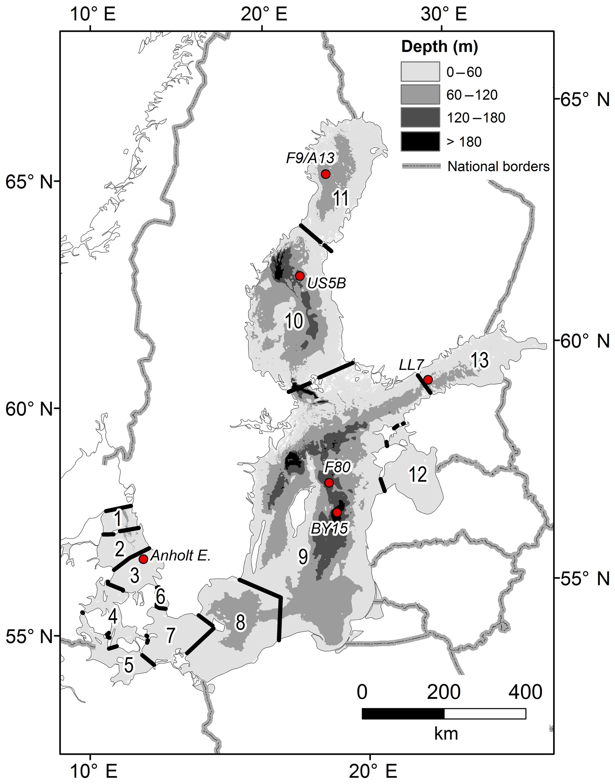
Figure 1The Baltic Sea area with sub-basins and monitoring stations. The sub-basins are (1) northern Kattegat (NK), (2) central Kattegat (CK), (3) southern Kattegat (SK), (4) Samsø Belt (SB), (5) Fehmarn Belt (FB), (6) Öresund (OS), (7) Arkona Basin (AR), (8) Bornholm Basin (BN), (9) Gotland Sea (GS), (10) Bothnian Sea (BS), (11) Bothnian Bay (BB), (12) Gulf of Riga (GR), and (13) Gulf of Finland (GF). Some BALTSEM sub-basins are aggregated into larger units in the budget calculations: the Kattegat (KT) includes sub-basins 1–3, the Danish Straits (DS) includes sub-basins 4–6, the Baltic Proper (BP) includes sub-basins 7–9, and the entire Baltic Sea (EBS) includes all sub-basins.
Based on available observations, present-day riverine TA loads to the Baltic Sea amount to ∼470 Gmol yr−1 (Gustafsson et al., 2014b, their Table 3). Using budget calculations, Gustafsson et al. (2014b) estimated that an additional TA source of 344 Gmol yr−1 is necessary to close the Baltic Sea TA budget. Approximately 260 Gmol yr−1 of this source cannot be explained so far. Of the 84 Gmol yr−1 that was resolved, 66 Gmol yr−1 resulted from the net effect of primary production, aerobic mineralization, and denitrification – essentially N cycling. The remaining 18 Gmol yr−1 resulted from net reduction ( reduction – dissolved sulfide () oxidation) in the water column, but this fraction could be reversed in case of oxygenation of the water column. It was hypothesized that a significant fraction of the unresolved TA source could be coupled to burial of Fe sulfides as a result of anaerobic mineralization in sediments. This would then represent a fraction of the reduction that is not readily reversed through ΣH2S oxidation upon reoxygenation of the water column. Due to incomplete descriptions of benthic processes in the model that was used, this hypothesis could not be tested (Gustafsson et al., 2014b), but the process has recently been identified as an important TA source in the Gdańsk Deep (Łukawska-Matuszewska and Graca, 2018).
The amount and form of Fe solids entering the sediment is a key factor controlling net benthic TA generation from Fe sulfide burial. Recent work on Fe dynamics in deep Baltic Sea basins has shown that the lateral transfer (“shuttling”) of Fe from shelves to deep basins is most intense when bottom water hypoxia is intermittent (Lenz et al., 2015a). Under such conditions, dissolved Fe can escape from the shelves, rather than being retained in the sediment as Fe oxides (in the case of oxic bottom water conditions) or Fe sulfides (in the case of widespread anoxia or euxinia). This Fe is then transported laterally to the deep basins, where local redox conditions determine its fate. The present-day low oxygen concentrations in many deep basins of the Baltic Sea promote reduction (Reed et al., 2016), indicating enhanced net benthic TA generation due to S burial as the escaped Fe reaches these basins. Sediment records of S concentrations can be used to calculate S burial and thus quantify the TA source associated with this burial.
Here, we use burial rates of solid phase S from the literature (Lenz et al., 2015b) and results from two different types of biogeochemical models to (1) constrain the present-day sedimentary TA release from Baltic Sea sediments to the water column, (2) quantify the large-scale changes in sedimentary TA release coupled to changes in eutrophication and oxygen conditions, (3) quantify the relative influence of different processes that contribute to the sedimentary TA release, and (4) estimate the potential future development of TA and pH levels upon recovery from eutrophication and assuming continued eutrophication. The models employed in this study are a high-resolution reactive-transport sediment model (RTM) (Reed et al., 2016) and a long-term, large-scale coupled physical–biogeochemical model for the Baltic Sea, BALTSEM (Gustafsson et al., 2017).
2.1 Data
2.1.1 Sediment data and calculations
Sedimentary alkalinity generation due to S burial in the Baltic Proper (sub-basins 7–9 in Fig. 1) was estimated using published data of S contents at F80, a 191 m deep site in the Fårö Deep of the Gotland Sea (Fig. 1; Lenz et al., 2015b). Concentrations of S in micromoles per gram (µmol g−1) were first converted to units of micromoles per cubic centimeter (µmol cm−3) using measured porosities and a sediment density of 2.65 g cm−3, which is typical for such sediments, and were subsequently depth-integrated between 0 and 25 cm in sediment depth. Following the age model presented by Lenz et al. (2015b), this depth interval represents the burial since 1970, allowing the calculation of an annually averaged rate of S burial (mmol m−2 yr−1). Using a 1:2 ratio between S burial and TA generation, the latter was calculated and subsequently extrapolated to the basin scale using the total muddy sediment area for the Baltic Proper (Table 1; Al-Hamdani and Reker, 2007).
Table 1Total sediment areas and muddy sediment areas (1000 km2). The muddy sediment areas are based on Al-Hamdani and Reker (2007). Sub-basins according to Fig. 1.

Although total S concentrations do not indicate in which form S is buried, this does not matter for the associated TA generation. The conversion from to reduced sulfur produces 2 mol of TA (in the form of ) per mole of S (Reaction R1, CH2O represents simplified organic matter). This is irrespective of whether it ultimately ends up in the form of Fe monosulfides (FeS), pyrite (FeS2), or elemental sulfur (S0) when being converted to a solid form. Reductive dissolution of Fe oxides also produces 2 mol of TA (as ) per mole of dissolved iron (Fe2+) formed, but this is compensated for when Fe2+ subsequently reacts with dihydrogen sulfide (H2S) during FeS formation, thereby releasing protons (Reaction R2). Therefore, there is no net TA generation associated with the formation of Fe2+ and its subsequent burial as Fe sulfide minerals (Hu and Cai, 2011a).
2.1.2 Oceanographic data
Measured TA and salinity in the 1970–2014 period were extracted from the ICES oceanographic database (ICES Data Set on Ocean Hydrography, the International Council for the Exploration of the Sea, Copenhagen, http://ocean.ices.dk/Helcom/, last access: 8 November 2016) and the Swedish Ocean Archive (SHARK) database provided by the Swedish Meteorological and Hydrological Institute (SMHI; http://sharkweb.smhi.se/, last access: 2 November 2016).
During the Swedish monitoring cruises water samples were at least occasionally stored in glass bottles with a head space of air until later analysis in the laboratory. This means that the ΣH2S in the samples may have been oxidized by the time of analysis (see Ulfsbo et al., 2011), which then implies that the reported TA concentrations in anoxic water can be substantially underestimated. For that reason, following Ulfsbo et al. (2011) we have adjusted the measured TA concentrations in euxinic waters by adding the ΣH2S concentration multiplied by a factor of 2 (i.e., ). However, if the ΣH2S was not removed by the time of analysis, the adjusted TA concentration would be too high.
2.1.3 River data
Riverine TA concentrations in the BALTSEM model were based on monthly measurements in 1996–2000 from 82 of the major rivers entering the Baltic Sea, representing approximately 85 % of the total runoff (see Gustafsson et al., 2014b). In this study we also include measurements from Swedish and Finnish rivers for the periods 1985–2012 and 2001–2012, respectively. Swedish chemical data were provided by the Swedish University of Agricultural Sciences (SLU; http://www.slu.se/en/, last access: 7 June 2016), and Swedish runoff data were provided by the SMHI (http://vattenwebb.smhi.se/, last access: 7 June 2016). Finnish data were extracted from the database Hertta provided by the Finnish Environment Institute (SYKE).
2.2 Model calculations
2.2.1 Sediment reactive-transport model (RTM)
A one-dimensional RTM (Reed et al., 2016) was used to calculate benthic TA generation and release at F80, with a minor modification: the redox reaction equations as presented in Table S8 by Reed et al. (2016) were updated to include the total concentrations of the ammonium and sulfide acid–base systems, instead of the corresponding acid–base species. The model calculates acid–base speciation using the direct substitution approach (Hofmann et al., 2008), in which pH and total quantities (dissolved inorganic carbon (DIC), ΣH2S, total ammonium (), etc.) are used as state variables, meaning that TA is calculated as an output variable. Effluxes of TA from the sediment were subsequently calculated from the gradient in the diffusive boundary layer (Boudreau, 1997). The model includes the carbonate, sulfide, ammonium, and phosphate acid–base systems, such that TA is defined as
The RTM thus ignores contributions of the fluoride, borate, and silicate acid–base systems, as well as the hydroxide ion and phosphoric acid, which make up part of the classical definition of TA (Dickson, 1981) but were expected to have a low contribution to TA in this setting. Moreover, the model neglects organic alkalinity, which can substantially contribute to Baltic Sea pore water TA (Łukawska-Matuszewska, 2016; Łukawska-Matuszewska et al., 2018), but which is challenging to calculate due to the variety of acid–base groups associated with organic matter. Further details on the governing equations, redox and equilibrium reactions, reaction parameters, and boundary conditions are given in Tables S1–S2 and S4 (Supplement) and in Reed et al. (2016).
The RTM has previously been used at this location to assess the impact of shelf-to-basin Fe shuttling on the formation and stability of the Fe(II) phosphate mineral vivianite (Fe3(PO4)2•8H2O; Reed et al., 2016). To this end, it was calibrated against a wide selection of pore water and solid phase data presented in Jilbert and Slomp (2013), Lenz et al. (2015b), and Reed et al. (2016). We confirm this calibration for the carbonate system with additional DIC and TA pore water data from a multicore recovered at F80 during a research cruise with R/V Pelagia in June 2016. Core handling and pore water analyses have been performed following Egger et al. (2016). We used the previous calibration and perform sensitivity analyses to identify the key mechanisms responsible for benthic TA generation and release. To represent the variety of bottom water conditions at site F80 since the 1970s, four time intervals were recognized (Fig. 2): 1970–1973 (baseline; I), 1973–1978 (start of change in Fe loading; II), 1978–1981 (eutrophication but pre-euxinia; III), and 1981–2009 (eutrophication and euxinia, IV).
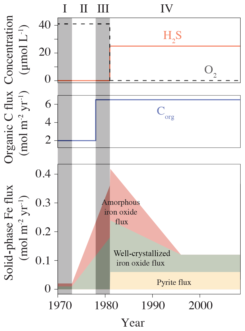
Figure 2Variability in bottom water redox conditions, organic carbon, and Fe inputs between 1970 and 2009, used to force the reactive-transport model at site F80. Numbers indicate the four different time intervals recognized in this study: (I) baseline (1970–1973), (II) start of change in Fe loading (1973–1978), (III) eutrophication but pre-euxinia (1978–1981), and (IV) eutrophication and euxinia (1981–2009). Figure modified from Reed et al. (2016).
2.2.2 Large-scale physical–biogeochemical model
BALTSEM is a coupled physical–biogeochemical model developed for the Baltic Sea. The model divides the system into 13 connected sub-basins (Fig. 1), for which each basin is described as horizontally homogeneous although with a high vertical resolution and a depth-dependent area distribution based on the real hypsography of the various sub-basins. A hydrodynamic module simulates mixing and advection (Gustafsson, 2000, 2003), while the dynamics of nutrients and plankton (Gustafsson et al., 2012, 2017; Savchuk et al., 2012) as well as organic carbon and the carbonate system processes (Gustafsson et al., 2014a, b; 2015) are simulated in a coupled biogeochemical module. The hindcast model simulations cover the period 1970–2014, while the scenario runs (Sect. 4.5) cover the period 1970–2099.
In BALTSEM, TA is based on Dickson (1981) but also includes the influence from organic alkalinity in the water column based on Kuliński et al. (2014) and Ulfsbo et al. (2015) (see Gustafsson et al., 2015):
Most biogeochemical processes related to production and mineralization in the water column and sediments either produce or consume TA. Many of these TA sources and sinks have been described in detail by Wolf-Gladrow et al. (2007) and Krumins et al. (2013). TA production and consumption resulting from processes such as ammonium-nitrate-based production, nitrification, denitrification, reduction, and ΣH2S oxidation are included in the BALTSEM calculations (Gustafsson et al., 2014b). All biogeochemical reactions that produce or consume TA in BALTSEM are given in Table S3 (Supplement). Under euxinic conditions in the water column, reduction and also accumulation represent large TA sources; these are, however, reversed if the water is again oxygenated by deep water inflows and vertical mixing. BALTSEM does not include Fe cycling, and in particular there are no parameterizations for Fe shuttling and subsequent burial of Fe sulfides in the sediments.
As mentioned in the introduction, observed river loads of TA are not sufficient to reproduce observed TA in the Baltic Sea. The additional source that is required can partly be explained by biogeochemical processes but is as yet largely unknown. This “unresolved source” was calibrated by Gustafsson et al. (2014b), and although the magnitude is well constrained, it has as yet not been possible to determine what the source is. The BALTSEM model has since been updated with both new processes and new forcing files. The model now includes the influence from acidic depositions based on Claremar et al. (2013). Furthermore, the forcing files now cover the period 1970–2014. As a result of these updates, the calibrated unresolved TA sources have been slightly modified in the present study compared to those by Gustafsson et al. (2014b) (see Sect. 3.2).
The processes behind the unresolved TA source are not known, but there are two candidates: external loads (e.g., river loads and submarine groundwater discharge) and internal processes (pelagic and/or benthic). In theory, the source could be associated with both processes that are not included in the model (e.g., Fe–S cycling, submarine groundwater discharge) and processes that are included but possibly not correct (e.g., river loads, nutrient cycling). Instead of speculating about contributions from various sources in the different sub-basins, we will perform two different scenarios: one case in which the unresolved source is added as additional land loads and one case in which the source is added as sediment release. The magnitudes of unresolved sources in different sub-basins are identical in the two cases.
Following Gustafsson et al. (2014b), no additional unresolved TA sources were added to the Kattegat and Danish Straits (sub-basins 1–6, Fig. 1). Since these basins have quite short residence times (Gustafsson, 2000), internal TA generation will not significantly influence concentrations from conservative mixing between inflowing saline water from the North Sea and outflowing fresher waters from the Baltic Proper. For that reason, it is not feasible to constrain any unresolved sources in these areas, although the same processes that generate TA in the remaining Baltic Sea should apply to these sub-basins as well.
2.2.3 Merits and limitations of using two models
Using a mass-balance approach, BALTSEM connects external sources, transports between basins, and internal cycling of carbon, nutrients, and TA within each sub-basin. The model is thus highly useful to quantify fluxes – resolved as well as unresolved – on basin and system scales. It is furthermore an invaluable tool when investigating multi-stressor effects on the ecosystem in future scenario calculations. However, the lack of parameterizations for TA production and consumption related to sedimentary Fe–S cycling means for example that there is no S burial – a process that represents a net TA source. The RTM, however, resolves these processes in detail and quantifies the fluxes at specific sites. It is not feasible to upscale such site-specific fluxes to the system scale. Moreover, it would require that the fate of all components contributing to the TA efflux calculated by the RTM should be evaluated in BALTSEM. We know that a substantial part of the TA efflux from the sediment is due to components that are reoxidized in the water column. Only a full coupling between both models, which is currently not feasible as discussed below, would allow us to monitor the fate of these components. We therefore use only that part of the TA efflux that is due to a sedimentary source that is permanent on the timescale of interest, i.e., the burial of reduced S. In the present study, the amount of S burial in a specific year is assumed to represent a release of TA from the sediments within that year. Given the relatively long timescale that we are looking at (averages over multiple years) compared to the actual rate of formation, we can assume that all TA associated with S burial will have diffused upwards and escaped the sediment. This TA flux due to S burial and computed by the RTM was subsequently upscaled to cover a certain bottom type in the relevant sub-basin (i.e., the total muddy sediment area). This was performed by multiplying the net TA generation resulting from S burial (mmol m−2 yr−1) by the muddy sediment area of the Baltic Proper (Table 1).
The RTM calculations provide the first estimates of the impact of benthic Fe–S processes on TA in the Baltic Sea, and in particular clarify to what extent the previously mentioned unresolved sources can be associated with S burial. Other processes that influence TA (e.g., redox reactions involving N) are included in both models. Although benthic N cycling is described in more detail in the RTM, it is in this case preferable to use the fluxes as calculated by BALTSEM. One reason is to take advantage of the coupled physical–biogeochemical approach as described above, so that the source of the can be identified on a basin scale. Moreover, denitrification rates at F80 are not representative for the entire sub-basin.
Ideally the RTM would be dynamically coupled to BALTSEM, but this is currently not feasible for two reasons: first and foremost, direct coupling would require that the state variables used in the two models would have to match so that the same reactions can be simulated in both models. This means that we would have to add numerous new state variables to BALTSEM (see Tables S1–S3). For each new state variable BALTSEM would furthermore need external loads and boundary conditions. Implementation of a full coupling between the two models is in other words a massive task and far beyond the scope of this study. Second, BALTSEM has approximately 1400 sediment “boxes”, and the RTM would have to compute the sediment processes in each of these boxes – calibration of the RTM in various parts of the Baltic Sea would be problematic because of an insufficient coverage of sediment data. Therefore, the two models are not directly coupled to one another but instead used independently.
3.1 Sediment and RTM calculations
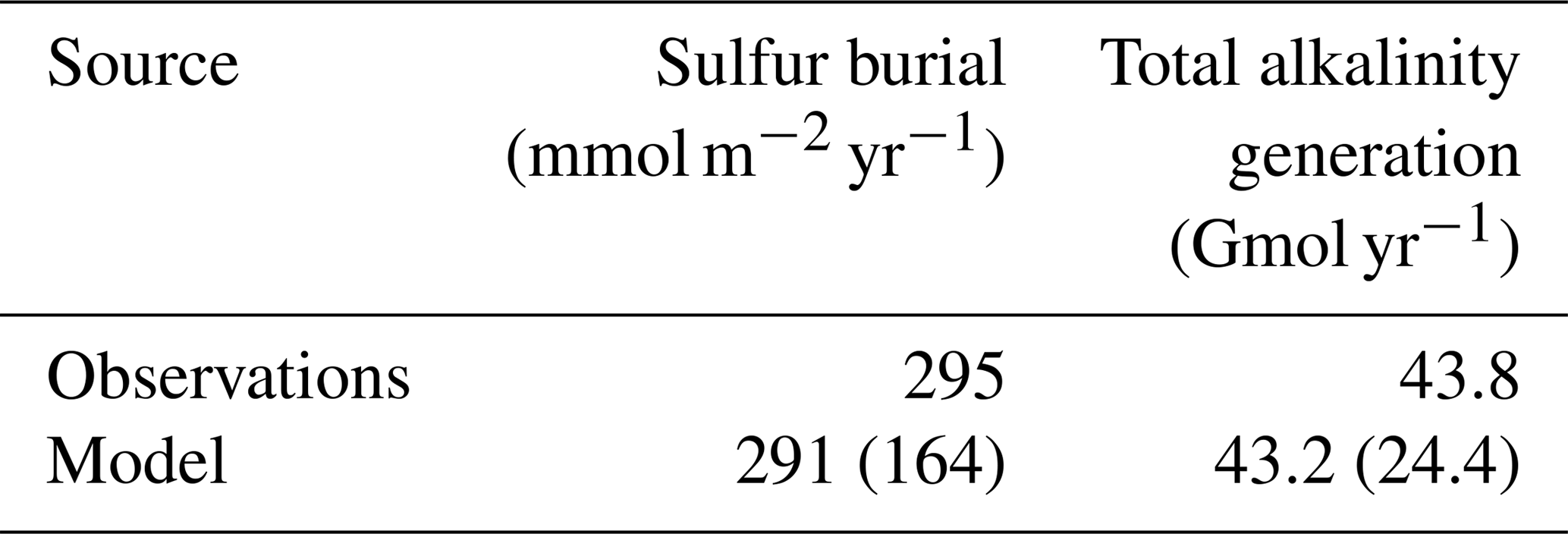
Both the model- and observation-based estimates indicate that between 1970 and 2009, on average 291–295 mmol S m−2 has annually been buried, leading to a TA generation of 582–590 mmol m−2 yr−1. This corresponds to a TA flux of ∼43.2–43.8 Gmol yr−1 from muddy sediments (Table 2). The model further suggests that virtually all of the S solids are present in the form of FeS2. Of the 291 mmol m−2 yr−1 of S being buried, only 56 % was formed in situ, whereas the remaining 44 % was deposited as a result of the shuttling of Fe in the form of FeS2 to the deep basin (Lenz et al., 2015a). However, as BALTSEM does not resolve FeS2 formation in either the water column or sediment, both need to be included when estimating the unresolved TA source due to reduction and S burial.
Table 2Estimated S burial (mmol m−2 yr−1) and associated TA generation (Gmol yr−1) for site F80 (lat 58.0000, long 19.8968) between 1970 and 2009. Both S contents and dating were taken from Lenz et al. (2015b). The basin-scale calculation was based on the total muddy sediment area for the Baltic Proper in BALTSEM of 74 300 km2 (Table 1). Numbers in parentheses represent S burial due to in situ S formation only, thus excluding S burial due to FeS2 deposition.
In line with other studies (e.g., Jørgensen, 1977), the vast majority of reduced S produced through reduction was reoxidized in either the sediment or the overlying water. On average, only 10.2 % was buried, but there was strong temporal variability in this percentage (Table 3). The fraction of S solids being buried was highest under eutrophic but non-euxinic conditions (i.e., period III; 40.7 %). Since 1981 (period IV), inputs of Fe oxides have decreased, leading to a higher efflux of ∑H2S and thus less S burial, despite higher reduction rates (SRRs). Our results indicate that even under non-euxinic conditions, pyrite formation was limited by the availability of highly reactive Fe, as is the case in most marine systems (Berner, 1984; Raiswell and Canfield, 2012). This limitation was confirmed by the difference between potential and simulated S formation rates (Table 3), for which the former indicates the amount of solid S that could have formed based on the other modeled sources and sinks of ∑H2S. It is thus indicative of the amount of S mineral formation under unlimited Fe2+ supply.
Table 3Estimated depth-integrated reduction (SRR), S reoxidation (S-OX), and S0 disproportionation rates (S0−dispr), as well as ∑H2S efflux (all in mmol S m−2 yr−1), as derived from the one-dimensional reactive-transport model (Reed et al., 2016) for the periods 1970–1973 (baseline; I), 1973–1978 (start change in Fe loading; II), 1978–1981 (eutrophication but pre-euxinia; III), and 1981–2009 (eutrophication and euxinia; IV). The difference between SRR (production of reduced S) and the sum of S-OX, S0−dispr, and ∑H2S efflux (removal of reduced S) is assumed to be representative for the maximum potential S formation. The simulated S formation is derived from the mass balance of the RTM (see Table S6 for details).
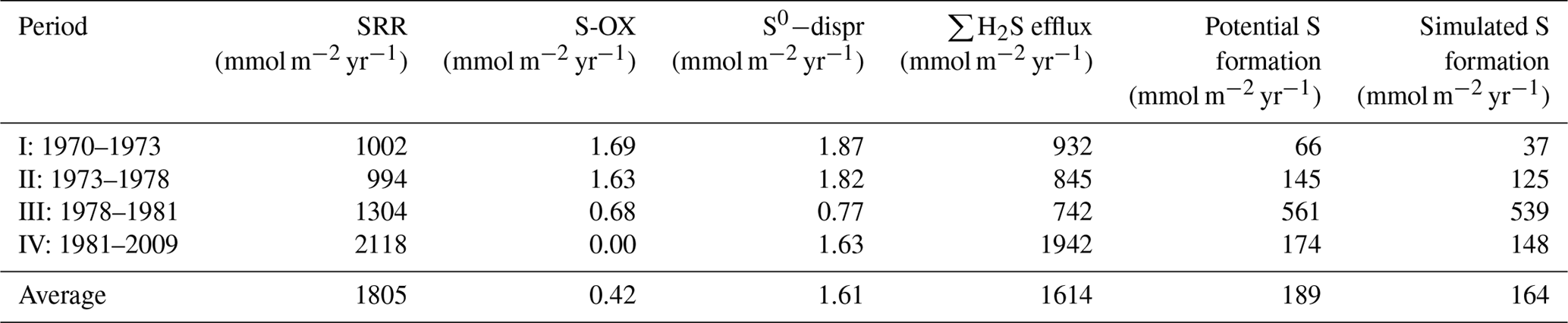
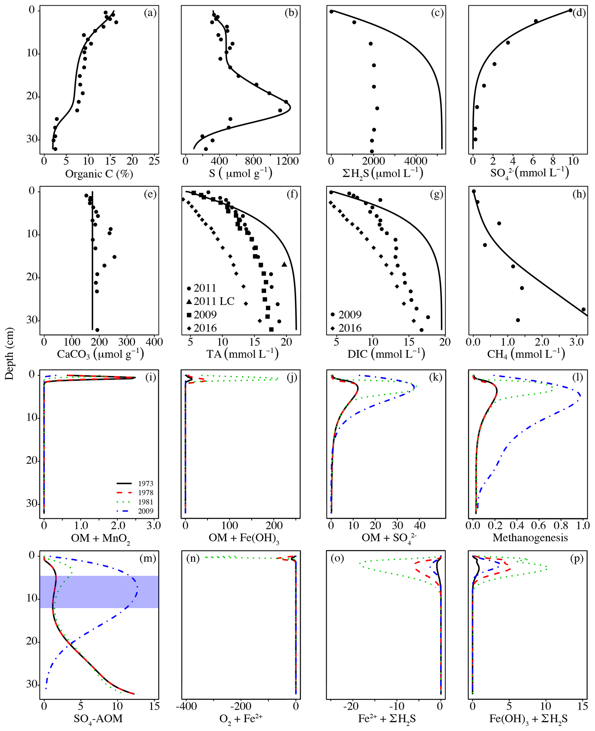
Figure 3Pore water profiles of selected simulated (solid lines) and observed (dots) variables at site F80 (a–h); simulated rates of some major processes impacting TA dynamics at the end of the four major time intervals (i–p; all rates in mmol TA dm−3 yr−1). The blue area in (m) indicates the sulfate–methane transition zone (SMTZ) in 2009; in the other years, the SMTZ was located around the depth of the modeled interval (32 cm). Additional pore water and solid phase profiles were published in Reed et al. (2016). Previously unpublished measurements can be found in Table S5 (Supplement). Dates in (a)–(h) indicate sampling dates; LC: long core.
In the period 1970–2009, S burial could on average only explain 328 mmol m−2 yr−1 of TA generation (Table 3; using a 1:2 ratio between S burial and net TA generation). This was 9.2 % of the internally generated TA (3948 mmol m−2 yr−1), but again clear temporal variations were observed (Table 4). Under the baseline conditions (period I), when little S was buried, it only made up 3.7 % of the total TA generation. This percentage increased to 12.4 % between 1973 and 1978 (period II), when more Fe was available, and peaked at 34.5 % between 1978 and 1981 (period III), when both Fe(OH)3 and carbon loadings were high. Since 1981 (period IV), the decrease in Fe(OH)3 loading has further limited S burial, leading to a contribution of only 6.7 % of the internally generated TA.
Pore water profiles of DIC and TA (Fig. 3f, g) indicate that the model is generally well calibrated for the carbonate system. Both DIC and TA concentrations were lower in 2016 compared to the earlier measured data against which the model was calibrated (Reed et al., 2016). The profiles furthermore show that the model overestimates the buildup of ∑H2S (Fig. 3c). This can be explained by loss of ∑H2S during sampling, which is a common problem for anoxic sediments, but also by the chosen lower boundary condition of the model. Whereas the model assumes no gradient with the underlying sediment, the data for 2009 (Jilbert and Slomp, 2013; Lenz et al., 2015b) show a declining trend with depth below 32 cm, suggesting a downward diffusive flux of ∼144 mmol ∑H2S m−2 yr−1 in 2009. When fixed at depth as Fe sulfides, this flux would lead to an additional TA generation of ∼288 mmol m−2 yr−1 for 2009. However, given the lack of major S accumulation in the sediment below 32 cm (Jilbert and Slomp, 2013), we do not believe this downward flux contributed greatly to net TA generation over the full period of investigation.
Table 4Estimated TA generation from the reactive-transport model integrated over the whole sediment column for the periods 1970–1973 (baseline), 1973–1978 (start change in Fe loading), 1978–1981 (eutrophication but pre-euxinia), and 1981–2009 (eutrophication and euxinia) for the dominant processes, as well as TA generation and efflux (all in mmol m−2 yr−1).

Rate profiles of the most important processes contributing to TA (Fig. 3i–p). show that especially between 1978 and 1981 (period 3), when OM and Fe inputs were high but bottom waters were still oxic, intense cycling of Fe occurred in the sediments, associated with high TA production and consumption. Dissolved Fe produced from reductive dissolution of amorphous Fe oxides during OM degradation either diffused upward, where it reoxidized in the oxic sediments (Fig. 3n), or downward to react with ∑H2S (Fig. 3o). Well-crystallized Fe oxides, assumed to be inaccessible for OM degradation, reacted with ∑H2S over a wide range, thereby producing additional Fe2+ (Fig. 3p).
On a system scale, this cycling of Fe does not lead to net TA generation (Hu and Cai, 2011a), but it may impact the efflux of alkalinity from the sediment that is calculated by the RTM. This flux cannot directly be used to assess the long-term net TA generation that we are interested in, as it is the product of a variety of reversible and irreversible TA-generating reactions, such as the intense Fe cycling discussed above. Moreover, its constituents (e.g., HS−) may become reoxidized in the water column. However, the magnitude and temporal variability in the efflux compared to those of S burial and total TA generation may provide information on its driving processes. Note that the difference between total TA generation and efflux (Table 4; Fig. 4) reflects the buildup of TA in the sediment, as well as loss of TA at depth through burial.
A comparison of their temporal variabilities shows that the benthic TA efflux only partly followed the pattern in S burial (Fig. 4; Table 3). Since 1973, when the efflux was 1901 mmol m−2 yr−1, it decreased to 1561 mmol m−2 yr−1 in 1978, followed by a sharp increase to 3261 mmol m−2 yr−1 in 1982 and a more gradual increase to 4823 mmol m−2 yr−1 in 2009. Generation of TA throughout the entire sediment column contributed to the calculated efflux (Table 4), to a major extent due to high rates of reduction at depth (Fig. 3k, m). The methane diffusing upward from deeper sediment layers played a key role here, being responsible for on average ∼95 % of the CH4-driven reduction and ∼43 % of the total reduction. The temporal change in spatial pattern of the CH4-driven e reduction (Fig. 3m) is a direct result of more being consumed by organic matter degradation since the start of bottom water euxinia (Fig. 3k, Table 4). This is confirmed by the upward-shifting sulfate–methane transition zone (SMTZ) since the onset of bottom water euxinia (Fig. 3d; see also Reed et al., 2016), whose position matches the highest reaction rates of CH4-driven reduction (Fig. 3m). The minor peak in CH4-driven reduction around 5 cm in depth in 1973 and 1978, and the slightly more pronounced peak at ∼3 cm in depth in 1981, are in contrast driven by in situ produced methane due to methanogenesis (Fig. 3l).

Figure 4Calculated TA efflux and generation at site F80 integrated over the whole sediment column (all in mmol m−2 yr−1) due to various biogeochemical processes implemented in the RTM.
Interestingly, the decrease in efflux between 1973 and 1978 (period II), which resulted from changes in the Fe loading, was not mimicked in either the total TA generation or the amount of S burial. Rather, it reflected the pattern of the change in TA generation through secondary reactions (Fig. 4). The most important secondary reaction contributing negatively to TA between 1973 and 1978 was the reoxidation of Fe2+, the rate of which more than doubled during this period (Table 4) and which, in contrast to the other dominant reactions, was restricted to the upper centimeter of the sediment column (Fig. 3n). This indicates that it was the driving force of the lower TA efflux during this period. Although reoxidation of Fe2+ consumed even more TA in period III (1978–1981), this was more than compensated for by the concurrent enhanced TA generation due to OM degradation, especially coupled to Fe-oxide reduction, even though that occurred deeper in the sediment (Fig. 3j; Table 4).
Table 5Average resolved and unresolved TA sources minus sinks (SMS) and river loads with standard deviations (Gmol yr−1) in 1970–2014 according to the BALTSEM calculations in this study. Sub-basins according to Fig. 1.


Figure 5Annual mean observed (dots) and modeled (lines) normalized surface water TA (TAN, µmol kg−1) and salinity in five sub-basins. Full and dashed lines represent the scenarios in which the unresolved TA sources are added as land loads or sediment release, respectively. Model data from sub-basins 3 (SK), 9 (GS), 10 (BS), 11 (BB), and 13 (GF) are compared to observed data at the Anholt East, BY15, US5B, F9/A13, and LL7 stations, respectively.
In summary, this discrepancy between sedimentary TA generation due to S burial and modeled effluxes of TA highlights that both represent processes acting at various spatial and temporal scales. Long-term TA generation should be interpreted as the net TA generation, i.e., the TA change occurring after all reoxidation reactions took place, in the coupled water column–sediment system. In contrast, calculated efflux of TA, as well as TA generation through various processes at a specific moment in time within different zones in the sediment, is highly variable and is directly impacted by local coupled dynamics of S, Fe, and CH4 (see also Table 4, Fig. 3). While the sedimentary processes are highly relevant to understanding the major factors driving short-term TA dynamics, ultimately it is the burial of S that represents a TA source relevant in the long term (see also Sect. 2.2.3).
3.2 BALTSEM calculations
The recalibrated unresolved TA sources as well as the resolved pelagic and benthic TA sources minus sinks in the different sub-basins as calculated with BALTSEM are indicated in Table 5. In total, the recalibrated unresolved source amounts to 260±0 Gmol yr−1 (constant over time), while the total resolved pelagic and benthic sources minus sinks amount to a net source of 120±47 Gmol yr−1 over the 1970–2014 period. For comparison, the riverine TA load amounts to 470±62 Gmol yr−1. In Figs. 5–6, simulated and observed surface and deep water TA normalized to mean salinity at the corresponding station and water depth (TAN) and salinity are shown. The normalized TA is used in order to avoid uncertainties related to discrepancies between simulated and observed salinity. Full lines in Figs. 5–6 represent the scenario in which the unresolved sources were added as land loads, whereas dashed lines represent the case in which these sources were instead modeled as sediment effluxes.
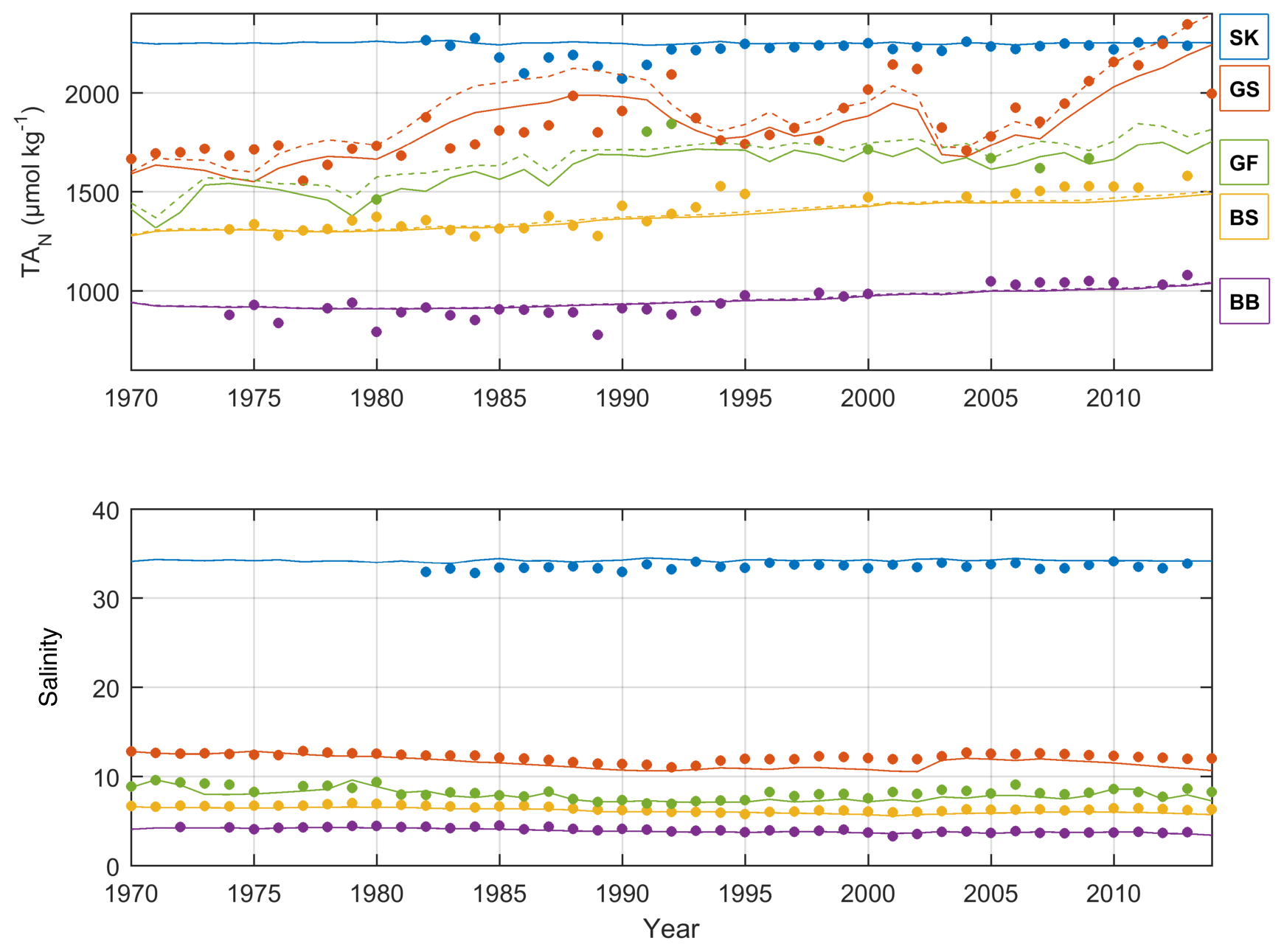
Figure 6Annual mean observed (dots) and modeled (lines) normalized deep water TA (TAN, µmol kg−1) and salinity in five sub-basins. Full and dashed lines represent the scenarios in which the unresolved TA sources are added as land loads or sediment release, respectively. Model data from sub-basins 3 (SK), 9 (GS), 10 (BS), 11 (BB), and 13 (GF) are compared to observed data at the Anholt East, BY15, US5B, F9/A13, and LL7 stations, respectively.
The temporal development of resolved and unresolved TA sources minus sinks throughout the model simulation is shown in Fig. 7. In this simulation, the unresolved sources in the different sub-basins were assumed to remain constant throughout the model run (Fig. 7), while the resolved sources and sinks vary depending on primary productivity, oxygen conditions, denitrification rates, and other biogeochemical processes included in the model. Despite the constant unresolved sources, simulated TAN concentrations generally reproduce observed values. Exceptions are the simulated TAN concentrations in the Kattegat and the Gotland Sea in the 1980s, where actual concentrations are overestimated, and TAN concentrations in the Bothnian Sea and Bay that are underestimated in the last 10-year period (Figs. 5–6).
There is an overall long-term increase in the resolved net TA generation in sediments and water column combined (Fig. 7), reflecting the ongoing eutrophication and overall deteriorating oxygen conditions of the Baltic Sea. The resolved net pelagic TA source increases in the period 1970–2000 in response to an increased primary production and then levels out and slightly declines in the last decade. The increased resolved benthic source in the last decade, however, is a response to deteriorating oxygen conditions resulting in increased TA generation through denitrification and reduction. Sulfate reduction in the BALTSEM model is however not an irreversible source since sulfidic waters can be reoxidized by deep water inflows, thus consuming TA and reversing the source.
4.1 Use of BALTSEM and RTM in the context of this work
Given the detailed presentation of sedimentary processes and effluxes in Sect. 3.1, one may wonder why only S burial is used in the coupling to BALTSEM. After all, the RTM calculations include many processes other than S burial. However, to study the impact of sedimentary TA generation on the long-term TA development in the Baltic Sea, we need to take into account only those processes that are relevant to accomplish this task.
BALTSEM includes many biogeochemical processes that produce and consume TA both reversibly and irreversibly on short timescales and in many boxes within each sub-basin of the Baltic Sea. These processes are described in Sect. 2.2.2 and are further listed in detail in Table S3. BALTSEM furthermore accounts for land loads, atmospheric depositions, and TA exchange between sub-basins and between the Baltic Sea and the North Sea. The result of the model simulations, i.e., the long-term development of TA in various sub-basins, is what we compare to observations in the water column (Figs. 5–6). Similarly, the RTM calculates net TA generation due to various reversible and irreversible processes (described in detail in Tables S1–S2). If we dynamically coupled the RTM to BALTSEM, we would have to consider all these processes and link all species between both models. Given the unfeasibility of this, as discussed in Sect. 2.2.3, we couple both models by using the output of the RTM to further constrain BALTSEM. Specifically, we explain part of the source of BALTSEM that is unresolved but necessary to describe the long-term TA development in the Baltic Sea.
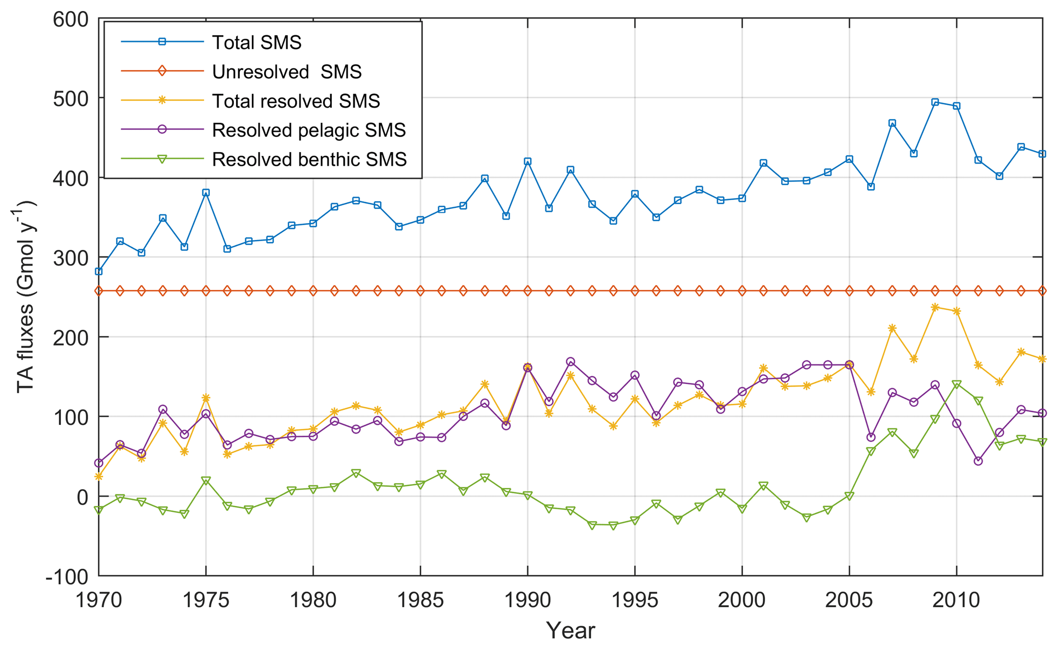
Figure 7Annual mean TA sources minus sinks (SMS) (Gmol yr−1) in the entire Baltic Sea according to BALTSEM calculations: Resolved benthic sources minus sinks (SMS) (green line), resolved pelagic SMS (purple line), total resolved SMS (yellow line), unresolved SMS (red line), and total SMS (blue line).
This means that in this context we only need to consider the processes from the RTM that are (a) irreversible on the timescale of interest (i.e., decades) and (b) not included in BALTSEM. Burial of Fe sulfides (Hu and Cai, 2011a) is the only major process that falls in this category. Denitrification using an external source, the other main pathway for net TA generation (Hu and Cai, 2011b), is already included in BALTSEM. Many other sedimentary processes produce or consume TA (Tables S1–S2, Supplement; Soetaert et al., 2007), but they are not irreversible on the relevant timescale. Their dynamics are, however, highly interesting to discuss as they help determine what limits net sedimentary TA generation and which processes mainly drive the effluxes of TA and other constituents to the water column. Note that this irreversibility is also a reason why we do not use these effluxes as input to BALTSEM. In addition, they are already partly included in BALTSEM, e.g., in the case of ∑H2S produced from reduction.
The RTM fluxes are upscaled under the assumption that the fluxes computed for the F80 site are representative for the muddy sediment area of the Baltic Proper. This assumption is associated with uncertainties because of spatial differences in the sediment geochemistry of muddy Baltic Proper sediments as illustrated by the pore water and Fe–S chemistry for four other sites as published by Lenz et al. (2015). The solid phase profiles for these sites show temporal trends over the past decades similar to those of F80. Furthermore, the pore water profiles show that site F80 has a relatively high rate of organic matter deposition and alkalinity regeneration when compared to most of the other sites. This implies that, with our extrapolation, the role of the sediment could be slightly overestimated. Thus, the large-scale fluxes we obtain by extrapolating fluxes from one specific site are to be regarded as a maximum estimate of the contribution of S burial to the overall TA budget of up to 26 %.
Although a full coupling between the two models is not a realistic goal at the moment, the development of sediment processes in BALTSEM is decidedly a highly desirable future goal. In particular, the inclusion of sedimentary Fe–S dynamics and related phosphorus (P) cycling would serve to improve our understanding of both TA and P dynamics on a system scale. The present study can be seen as an intermediate step towards a more detailed (if not complete) model description of sediment processes in the Baltic Sea. In fact, the relatively large influence of sedimentary processes on TA dynamics that we demonstrate in this study also serves as a motivation to pursue this goal.
4.2 Sulfur burial and TA generation in the Baltic Proper
While mineralization in the sediments occurs everywhere where there is labile organic matter, permanent burial of organic matter as well as other solids such as Fe sulfides should predominantly occur in muddy sediments. Consequently, the part of the unresolved TA source that is a result of S burial should be released from muddy sediments rather than from the entire sediment surface area of the Baltic Sea. Our RTM calculations in combination with observations from site F80 in the Baltic Proper (sub-basins 7–9 in Fig. 1) provide the first estimate of TA generation resulting from S burial in Baltic Sea sediments (582–590 mmol m−2 yr−1). Assuming that the calculated TA generation resulting from S burial is representative only for the muddy sediment area in the Baltic Proper (74 300 km2; Table 1), the total annual flux in this area is ∼44 Gmol yr−1. The calibrated unresolved TA source in the Baltic Proper amounts to 170±0 Gmol yr−1 according to the BALTSEM model (Table 5).
In the two different scenarios in which the unresolved source is added as land loads (full lines in Figs. 5–6) or sediment release (dashed lines in Figs. 5–6), the simulated surface water TA concentrations are very similar (Fig. 5). Deep water concentrations, however, differ significantly in the Gotland Sea and the Gulf of Finland but not in the other sub-basins (Fig. 6). The reason behind the rather similar results for these two different scenarios is that land loads supplied to the different basins are rapidly distributed in the well-mixed surface layer, and the well-mixed surface layer constitutes a large majority of the water volume. In the deeper and more isolated parts of the system, TA concentrations are lower in the “land loads” case compared to the “sediment release” case.
In the sediment release case, the unresolved TA source in the Baltic Proper (170±0 Gmol yr−1) corresponds to a flux of 730 mmol m−2 yr−1 if the source is distributed evenly over the entire sediment surface (228 000 km2). However, if the unresolved source is instead constrained only to muddy sediments, the flux would amount to 2236 mmol m−2 yr−1, which is far above the long-term mean flux due to S burial as obtained by RTM calculations. Even during peak pyrite formation periods, S burial only resulted in a source of 1078 mmol TA m−2 yr−1 (Table 3). Furthermore, in a BALTSEM experiment in which the unresolved sources were released only from muddy sediments (but at higher rates corresponding to the smaller surface areas), the deep water TA concentrations in particular in the Baltic Proper were overestimated while the surface water TA concentrations were underestimated (not shown). Based on the RTM calculations, TA generation coupled to S burial could thus account for 26 % of the unresolved source, at least in this sub-area of the system. The remaining unresolved TA source of ∼74 % could possibly be explained by underestimated river loads or submarine groundwater discharge of TA (e.g., Szymczycha et al., 2014). We have no data to quantify these fluxes, however.
4.3 Reversible versus irreversible sedimentary processes generating TA
As demonstrated by both simulated and observed sediment profiles at F80, a transition from hypoxic to euxinic conditions around 1980 resulted in a strong increase in both solid phase S and Fe burial (Reed et al., 2016). Furthermore, the molar S-to-Fe ratio of ∼2 suggests formation and burial of mostly FeS2. Both FeS2 and FeS can be formed from reactive Fe2+ and sulfide produced during Fe(OH)3 and reduction, respectively. These redox reactions ultimately result in net TA generation (Tables S1–S2, Supplement). Another possible pathway is that methane (formed by methanogenesis) is oxidized anaerobically by reduction of either or Fe(OH)3 (Slomp et al., 2013; Egger et al., 2015b), and Fe and sulfide can then be sequestered in the form of FeS2. Results from the RTM indicate that CH4 and organic matter are both important electron donors at F80. CH4 oxidation contributes to, on average, 43.8 % of total SRR and occurs at greater depth than reduction through organic matter degradation (Fig. 3k, m). Iron-mediated anaerobic oxidation of methane is not included in the set of reactions of this RTM. Previous work has indicated that this process mainly occurs in organic-poor sediments depleted in (Riedinger et al., 2014; Egger et al., 2017). These conditions are not met at F80, rendering an important role for this process unlikely.
Apart from such eutrophication-induced changes in the coupled Fe–S cycling, increasingly euxinic conditions also influence manganese (Mn) sequestration in sediments. Dissolved Mn2+ can be sequestered in the form of Mn carbonates (MnCO3). If this occurs, the TA generation associated with the reduction of manganese dioxide (MnO2; 2 mol of TA per mole of MnO2; Tables S1–S2, Supplement) is completely compensated for by the TA sink associated with carbonate removal. However, under euxinic conditions, manganese sulfide (MnS) can be formed if the sulfide availability exceeds the Fe2+ availability (Lenz et al., 2015b). Indeed, long-term sediment records indicate a relation between euxinic periods in Baltic Sea deep waters and burial of Mn sulfides in the forms of both rambergite and alabandite (Lepland and Stevens, 1998). As opposed to burial of MnCO3, burial of MnS results in a net TA generation comparable to that of FeS2 burial. In the RTM, we did not investigate the possible impact of MnS formation on TA generation as the sediment record at F80 does not show substantial Mn enrichments in the surface, despite higher sulfide than Fe2+ availability (Lenz et al., 2015b).
Ammonium, ΣH2S, Fe2+, and Mn2+ are rapidly oxidized if oxygen is supplied to anoxic waters. The result is a TA sink that compensates for the TA generation by anaerobic mineralization. Precipitates such as FeS and FeS2 can also be oxidized but this is generally a slower process, especially in the case of FeS2 (Millero et al., 1987; Wang and Van Cappellen, 1996). Moreover, these S minerals are embedded in organic-rich, ΣH2S-producing sediments. This reduces the impact of possible reoxygenation of the sediment for extended periods of time, implying that the TA source that results from S burial is stable. Sediment cores indicate the presence of Fe sulfides – in particular FeS2 – in the top 3 m of Gotland Sea deep water sediments (Boesen and Postma, 1988) as well as in the top 10 m of deep Bornholm Basin sediments and the top 27 m of Landsort Deep sediments (Egger et al., 2017), all corresponding to roughly 8000 years. In our model results, FeS2 is the dominant form of S in the sediment. Our work also shows that reoxidation of reduced S never exceeds 0.5 % between 1970 and 2009, irrespective of whether S solids or the total reduced S pool (i.e., including ∑H2S) is investigated (Table S5, Supplement).
Vivianite formation is another process that generates TA in a net sense. The presence of vivianite in sediment cores (Egger et al., 2015a) indicates that this mineral can be stable upon burial. However, vivianite dissolves in the presence of ΣH2S (Dijkstra et al., 2018), excluding its burial to be a long-term TA source at F80. It could however be a stable TA source at locations where ΣH2S rather than Fe availability limits pyrite formation, such as the Bothnian Sea (Egger et al., 2015a).
Calcifying organisms that build calcium carbonate (CaCO3) shells have a large influence on the carbonate system in many marine areas, as illustrated by high TA fluxes related to CaCO3 formation and dissolution in the North Sea (Brenner et al., 2016). CaCO3 formation results in a TA drawdown in the productive layer and a TA source where the shells are dissolved. Burial of CaCO3 shells is a net TA sink on a system scale. In the Baltic Sea, however, planktonic calcifiers are largely absent – likely because of low saturation values of calcite and aragonite in winter (Tyrrell et al., 2008). In the RTM, CaCO3 dissolution and precipitation are included, based on observed sedimentary CaCO3 contents of ∼200 µmol g−1 (Fig. 3e; see Reed et al., 2016, for further details). The prescribed input of 86 mmol m−2 yr−1 in combination with prevailing conditions in the sediment led to a net TA loss due to CaCO3 dissolution, which is on average only −0.01 mmol m−2 yr−1 (data not shown). For this reason, we have not included the effects of CaCO3 precipitation and dissolution in our analysis.
4.4 Long-term development of TA in the Baltic Sea
Several studies indicate essentially linear TA–salinity relations in Baltic Sea surface water (Ohlson and Anderson, 1990; Thomas and Schneider, 1999; Perttilä et al., 2006; Beldowski et al., 2010). Long-term TA increases that are not connected to salinity are, however, apparent from observed TA–salinity relations (Fig. 8; Tables S7–S8, Supplement). Furthermore, Müller et al. (2016) found generally increasing TA concentrations decoupled from salinity in the Baltic Sea over the past 2 decades.
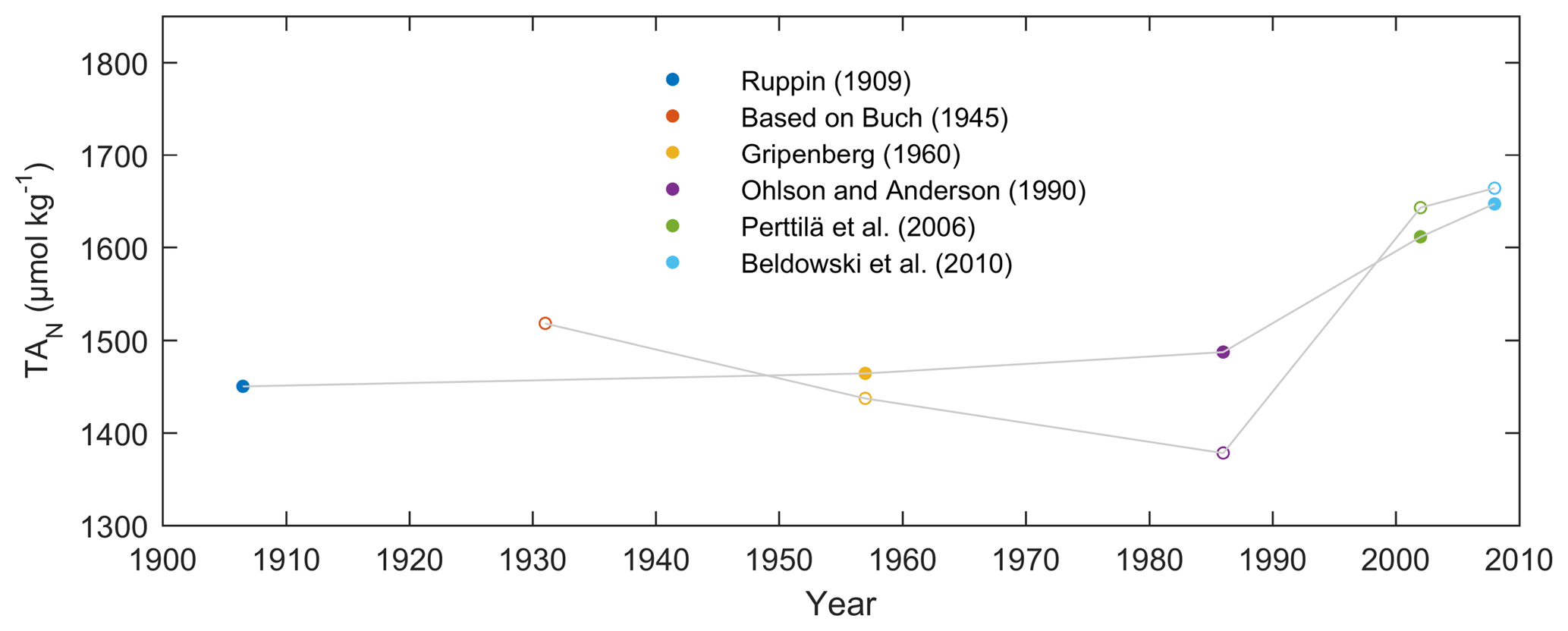
Figure 8TA concentrations normalized to salinity = 7 (TAN), using the TA–salinity relations for the Baltic Proper – Kattegat (full circles), and Baltic Proper – Gulf of Bothnia (open circles) (see Tables S7–S8, Supplement). The Ruppin (1909) value was based on measurements in 1906–1907 (see Dyrssen, 1993), while the Buch (1945) value was based on measurements in 1927–1935 (see Buch, 1945). The Buch (1945) and Perttilä et al. (2006) values were converted to micromoles per kilogram from micromoles per liter.
The resolved pelagic and benthic TA sources minus sinks in the BALTSEM calculations (Fig. 7) on average increase by approximately 3 Gmol yr−1 in the 1970–2014 period. Furthermore, the RTM calculations (Table 3) indicate that S burial can increase by a factor of 4 after a transition from oxic to anoxic/euxinic conditions, and even by an order of magnitude during this transition if both Fe-oxide and organic matter loadings are enhanced. Thus, the fraction of the unresolved source that is a result of S burial should be quite variable depending on mineralization rates and oxygen conditions in different areas of the Baltic Sea as well as during different periods in time.
Anaerobic mineralization occurs in sediments even if the overlying water is oxic, and for that reason TA release coupled to S burial does not exclusively occur from sediments covered by sulfidic waters. In fact, our results indicate the highest S formation rates under eutrophic, but non-euxinic, conditions (Table 3). However, large-scale and long-term changes in TA generation related to changes in S burial are mainly expected to occur in areas experiencing transitions between oxic and anoxic conditions and in addition as a result of changes in Fe loadings (Lenz et al., 2015a). Hypoxic and anoxic conditions in the Baltic Sea water column – as well as rapid transitions between oxic and anoxic conditions – occur primarily in the deep basins of the Baltic Proper, although episodes of oxygen depletion can also occur in the deep water of, in particular, the Gulf of Finland, as well as in many eutrophic coastal fjords and bays.
The long-term TA decrease in the Gotland Sea in the 1980s coincided with a decreasing salinity (Figs. 5 and S1) as well as improved oxygen conditions in large volumes of the deep water (not shown). During this period, stratification was considerably weakened and as a result the halocline depth in the Baltic Proper increased, and inflowing new deep water ventilated primarily the upper deep water. Thus, a much larger water volume than usual was well ventilated (e.g., Stigebrandt and Gustafsson, 2007). It is possible that during this period, S burial and associated TA generation were considerably weakened. A very strong TA increase observed in the early 1990s coincides (more or less) with a strengthened stratification due to saltwater inflows in 1993. A rapid deterioration of oxygen conditions followed because of a suppressed deep water ventilation during periods of strong stratification. This development towards increasingly anoxic/euxinic conditions could potentially cause a large response in terms of TA generation.
It is however likely that the observed TA decline in the 1980s followed by the strong TA increase in the 1990s is exaggerated because of unreliable measurements before 1993. After that, the precision of TA measurements appears to have increased considerably as is evident from the relatively low scatter in TA values after 1993 compared to before 1993 (see Müller et al., 2016, their Fig. 3). In particular, we find in Fig. 6 that even in the Kattegat deep water the observed TA concentrations in the period ∼ 1985–1992 are comparatively low. While the Kattegat surface waters are heavily influenced by outflowing Baltic Proper water, the Kattegat deep water is affected only very marginally. Furthermore, the observed TA values from the Gotland Sea deep water in approximately the same period are considerably lower than our modeled values (Fig. 6).
TA is also influenced by atmospheric deposition on the water surface due to emissions from land and ships (Hassellöv et al., 2013; Hagens et al., 2014). Deposition of S and N oxides represents a TA sink, while deposition is a TA source. The net effect is a TA sink; the impact peaked in the 1980s, but has since then diminished due to reduced land emissions (Omstedt et al., 2015). According to our BALTSEM calculations, the TA sink related to acidic depositions has declined from approximately −40 Gmol yr−1 in the 1980s to −10 Gmol yr−1 in the past decade. This reduced TA sink thus contributes to the increasing TA concentrations in the Baltic Sea.
Riverine TA concentrations can increase as a result of enhanced weathering of carbonate and silicate rocks in the catchments. The rate of weathering depends on temperature, precipitation, soil organic matter contents, and deposition of acids (Ohlson and Anderson, 1990; Dyrssen, 1993; Sun et al., 2017). Average TA loads from Swedish rivers in 1985–2012 and Finnish rivers in 2001–2012 amount to 42 and 15 Gmol yr−1, respectively (Fig. S2, Supplement), together corresponding to some 12 % of the total TA load (∼470 Gmol yr−1) to the system. There was a strong long-term increase in the flow-normalized TA loads from Swedish rivers – approximately 21 % over the period 1985–2012. In Finnish rivers, however, there was no increase in the period 2001–2012. Because of a generally poor availability of river data from other countries around the Baltic Sea, we have no clear understanding of the long-term TA development in the great rivers in the southeastern Baltic Sea (where the highest TA concentrations are also generally observed).
Riverine TA concentrations in the BALTSEM model were calculated from observed monthly mean values only in the period 1996–2000. If the long-term increasing trend observed for TA loads in Swedish rivers is also representative for rivers in the southeastern Baltic Sea, this would signify that the model is forced by too low riverine TA concentrations in the last decade but conversely too high concentrations in the first couple of decades. It is plausible that changes in river water properties are responsible for at least part of the overall increasing TA concentrations in the Baltic Sea. This could in particular be the case for the Bothnian Sea and Bay where simulated TA in the last decade is underestimated by the BALTSEM model (Figs. 5–6).
4.5 Simulations of future scenarios
High productivity and deep water oxygen consumption rates favor TA-generating anaerobic mineralization processes. One potential consequence is that a large-scale recovery from eutrophication could reduce the CO2 buffering capacity of a marine system and thus also reduce the atmospheric CO2 sink and surface water pH.
In this section we investigate how the simulated TA in BALTSEM responds to two different nutrient load scenarios: (1) the business-as-usual (BAU) scenario with high nutrient loads throughout the 21st century and (2) the Baltic Sea Action Plan (BSAP) scenario with large reductions in N and P loads (Fig. S3, Supplement). We use the ECHAM5 A1B no. 1 scenario for CO2 emissions and climate change downscaled for the Baltic Sea region (see Omstedt et al., 2012). The A1B emission scenario represents a socioeconomic development producing medium CO2 emissions for which the atmospheric CO2 partial pressure (pCO2) reaches some 700 µatm by the year 2100 (Fig. S4, Supplement). The unresolved TA source is kept constant throughout these simulations. This means that any simulated changes in TA are related to changes in river loads and exchange with the North Sea, as well as changes in TA-producing and TA-consuming biogeochemical processes that are included in BALTSEM (production, mineralization, denitrification, nitrification, reduction, ΣH2S oxidation, etc.).
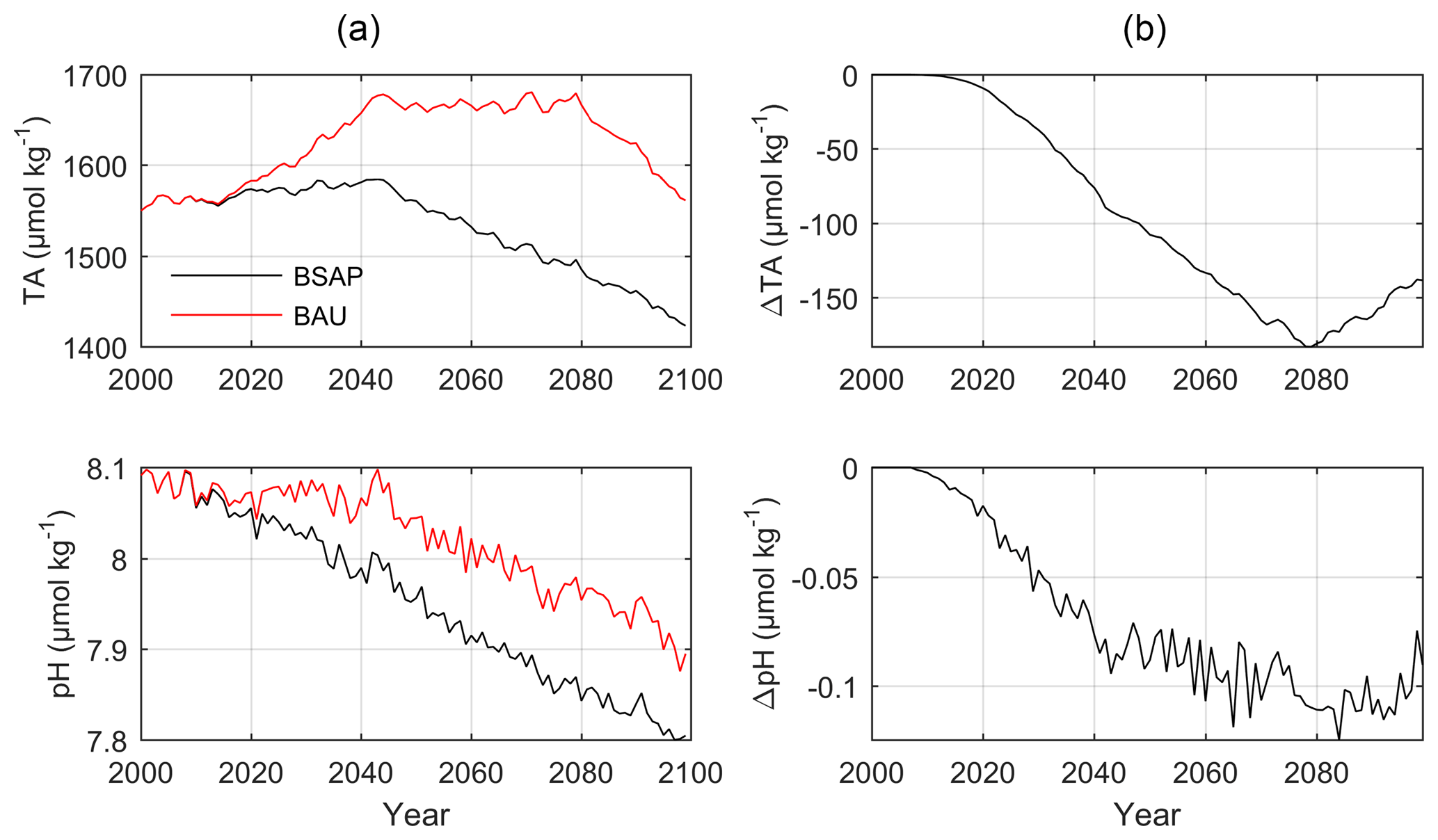
Figure 9(a) Simulated annual mean surface water TA and pH in sub-basin 9 (GS) according to the BSAP (black lines) and BAU (red lines) nutrient load scenarios. (b) Differences between the BSAP and BAU scenarios.
According to the BALTSEM simulations, the surface and deep water temperatures in the Gotland Sea will increase by approximately 3 ∘C over the 21st century, while salinity is reduced by more than 2 (Fig. S5, Supplement). Surface water phosphate concentrations will decline by ∼0.2 µmol kg−1 in the BSAP scenario, resulting in a reduced primary production and increased deep water oxygen concentrations (Fig. S6, Supplement). The reduced productivity and large-scale recovery from anoxic deep water conditions in the BSAP scenario will also have large consequences for TA and in extension CO2 buffer capacity and pH. Towards the final decades of the simulations, surface water TA in the BAU scenario exceeds that in the BSAP scenario by ∼150 µmol kg−1 (Fig. 9). As a result, the surface water pH is reduced by 0.1 units more in the BSAP than in the BAU scenario.
Table 6Input of Fe oxides and simulated S burial and TA efflux averaged for the period 2011–2050 under a range of environmental conditions as calculated with the reactive-transport model. All values are in mmol m−2 yr−1.
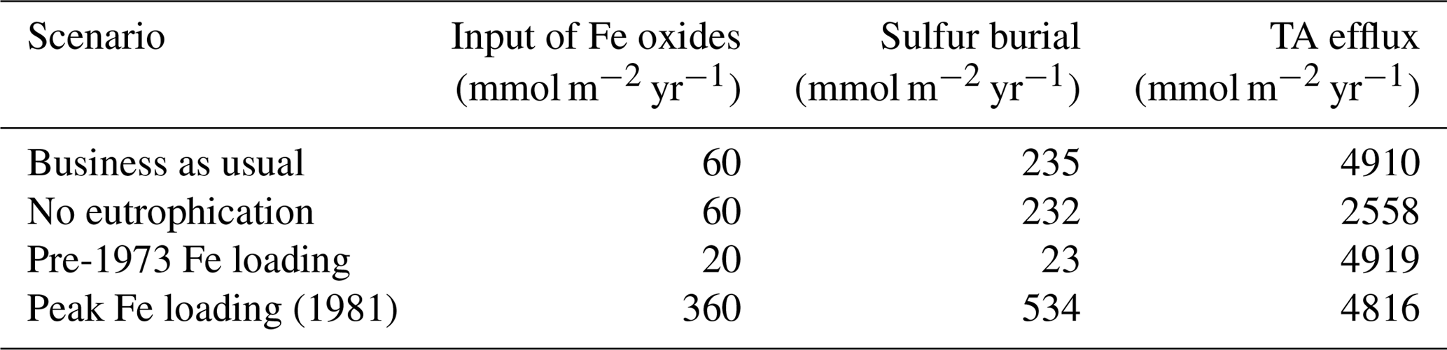
These scenario simulations do not include changes in TA generation resulting from changes in S burial driven by productivity and Fe-oxide availability since these processes are not resolved in BALTSEM. To investigate how the sediment, and more specifically S formation and burial, will respond to changes in Fe and organic carbon loadings, we ran the RTM for an additional 40 years under the present environmental conditions, as well as under a range of changes in these loadings. This sensitivity analysis (Table 6) shows that reverting the productivity regime to pre-1978 conditions decreases the calculated TA efflux by ∼50 %, a direct result of less organic matter degradation, whereas S burial is hardly impacted as it is still limited by Fe availability. Lowering the Fe-oxide loading to pre-1973 values decreases the S burial by an order of magnitude, confirming its limitation by Fe. Strikingly, the TA efflux is only marginally impacted, indicating again the decoupling between short-term flux dynamics and long-term TA generation, as discussed extensively in Sects. 2.2.3 and 3.1. Increasing the Fe-oxide loading to the peak values of 1981 slightly lowers the TA efflux while more than doubling S burial, a direct result of a higher Fe availability. In summary, our sensitivity analysis confirms that the form and rate of Fe input exerts the dominant control on S burial and long-term TA impacts, whereas the rate of organic matter input mainly drives the short-term variability in TA effluxes. It also highlights that sedimentary TA generation due to S burial and modeled effluxes of TA should be regarded as occurring on various temporal scales.
It is a simple exercise to examine the sensitivity of pH to further changes in TA. Using the CO2SYS software (van Heuven et al., 2011; http://cdiac.ess-dive.lbl.gov/ftp/co2sys/CO2SYS_calc_MATLAB_v1.1/, last access: 14 November 2016), and assuming that the surface water pCO2 is in equilibrium with the atmosphere, a surface water pCO2 of 700 µatm and TA of 1425 µmol kg−1 (as at the end of the BSAP scenario) results in a surface water pH of 7.80, assuming a salinity of 5.2 and temperature of 11 ∘C (see Fig. S5). For example, decreasing the surface water TA to 1325 or 1225 µmol kg−1 results in pH values of 7.77 or 7.73, respectively. Conversely, in order to completely compensate for the CO2-induced pH decline resulting from an atmospheric pCO2 increase to ∼700 µatm in the A1B scenario, the surface water TA would have to increase to approximately 2800 µmol kg−1 – which is a completely unrealistic TA concentration for surface water in the Gotland Sea regardless of productivity and oxygen conditions. It is for that reason beyond any doubt that the only possible way to avoid acidification of open Baltic Sea waters is to implement large reductions in CO2 emissions. Although there is a larger pH decline in the BSAP than in the BAU scenario, the possible negative influence must be considered to be of a marginal importance compared to the vast benefits for Baltic Sea ecosystems following reduced deep water dead zones.
Model calculations have been used to constrain the sedimentary TA efflux in the Baltic Proper and to examine how this efflux has developed over a 40-year period in relation to eutrophication and oxygen deterioration. In particular, the net TA source related to permanent S burial in the sediment was calculated using a reactive-transport model. Furthermore, the physical–biogeochemical BALTSEM model was used to estimate future TA concentrations and pH levels depending on the development of nutrient loads to the system.
The sedimentary TA generation undergoes large changes depending on both organic matter loads and oxygen conditions. Especially large changes occur during transitions between suboxic and euxinic conditions. Some of these changes are reversible, while others – such as a permanent S burial – result in a net TA generation. Our calculations imply that S burial in the Baltic Proper has resulted in an average net TA generation of up to 44 Gmol yr−1 in the period 1970–2009. This flux covers ∼26 % of the missing TA source in this basin (as estimated by the BALTSEM model).
When comparing the BAU and BSAP nutrient loads in combination with the A1B scenario for CO2 emissions, we find a larger pH reduction in the BSAP case than in the BAU case (by approximately 0.1 pH unit). This is a response to reduced signs of eutrophication and particularly substantial improvements in deep water oxygen conditions: in our calculations the gradual decline in anaerobic mineralization following improved oxygen conditions results in a reduced TA generation and thus a reduced buffer capacity for atmospheric CO2 in the Baltic Sea. Sedimentary S burial is not resolved in the BALTSEM model. Additional scenario calculations were for that reason performed with the RTM; the results indicate that S burial and long-term effects on the sedimentary TA efflux are primarily controlled by the Fe cycle, while short-term changes in the TA exchange between sediments and the water column mainly depend on organic matter inputs.
The RTM model code is available from Mathilde Hagens and Caroline P. Slomp upon request. Pore water DIC and TA data measured in 2016 are published in the Supplement of this paper and will be made available in the PANGAEA database. Other pore water and sediment data have been published before (Jilbert et al., 2011, 2012; Lenz et al., 2015c). The BALTSEM model code is available from Erik Gustafsson and Bo G. Gustafsson upon request.
The supplement related to this article is available online at: https://doi.org/10.5194/bg-16-437-2019-supplement.
EG, MH, CPS, and BGG designed the research. EG, MH, XS, CH, and CPS collected observational data. EG and BGG wrote the BALTSEM code. DCR and MH wrote the RTM code. EG and MH performed the model simulations. All authors interpreted the results. EG and MH wrote the paper with comments provided by all authors. EG and MH contributed equally to this work and thus share the first authorship.
The authors declare that they have no conflict of interest.
This article is part of the special issue “The 10th International Carbon Dioxide Conference (ICDC10) and the 19th WMO/IAEA Meeting on Carbon Dioxide, other Greenhouse Gases and Related Measurement Techniques (GGMT-2017) (AMT/ACP/BG/CP/ESD inter-journal SI)”. It is a result of the 10th International Carbon Dioxide Conference, Interlaken, Switzerland, 21–25 August 2017.
This study was supported by the TRIACID project funded by the Nordic Council
of Ministers (grant no. 170019) and BONUS COCOA funded by Formas and the
European Commission. The Baltic Nest Institute is supported by the Swedish
Agency for Marine and Water Management through their grant 1:11 – Measures
for marine and water environment. Further funding comes from the Netherlands
Organisation for Scientific Research (NWO; Vici 865.13.005 awarded to
Caroline P. Slomp) and the European Research Council under the European
Community's Seventh Framework Programme for ERC starting grant no. 278364.
Mathilde Hagens received additional financial support through the Dutch
Network of Women Professors (LNVH; DWS Fund 2016). We thank the captain and
crew of R/V Pelagia (64PE411) for their support and Matthias Egger,
Martijn Hermans, and Sharyn Ossebaar for their contributions to the collection
of the pore water DIC and TA data. Erik Smedberg and Annika Tidlund are
acknowledged for contributions to the artwork.
Edited by: Corinne Le Quere
Reviewed by: three anonymous
referees
Al-Hamdani, Z. and Reker, J.: Towards marine landscapes in the Baltic Sea, BALANCE Interim Report No. 10, available at: http://balance-eu.org/ (last access: 28 April 2017), 2007.
Andersson, A. J., Mackenzie, F. T., and Lerman, A.: Coastal ocean CO2 – carbonic acid-carbonate sediment system of the Anthropocene, Global Biogeochem. Cy., 20, GB1S92, https://doi.org/10.1029/2005GB002506, 2006.
Bauer, J. E., Cai, W.-J., Raymond, P. A., Bianchi, T. S., Hopkinson, C. S., and Regnier, P. A. G.: The changing carbon cycle of the coastal ocean, Nature, 504, 61–70, https://doi.org/10.1038/nature12857, 2013.
Beldowski, J., Löffler, A., Schneider, B., and Joensuu, L.: Distribution and biogeochemical control of total CO2 and total alkalinity in the Baltic Sea, J. Marine Syst., 81, 252–259, https://doi.org/10.1016/j.jmarsys.2009.12.020, 2010.
Berner, R. A.: Sedimentary pyrite formation: An update, Geochim. Cosmochim. Ac., 48, 605–615, https://doi.org/10.1016/0016-7037(84)90089-9, 1984.
Boesen, C. and Postma, D.: Pyrite formation in anoxic environments of the Baltic, Am. J. Sci., 288, 575–603, https://doi.org/10.2475/ajs.288.6.575, 1988.
Boudreau, B. P.: Diagenetic Models and Their Implementation, Springer Berlin Heidelberg, Berlin, Heidelberg, 1997.
Breitburg, D., Levin, L. A., Oschlies, A., Grégoire, M., Chavez, F. P., Conley, D. J., Garçon, V., Gilbert, D., Gutiérrez, D., Isensee, K., Jacinto, G. S., Limburg, K. E., Montes, I., Naqvi, S. W. A., Pitcher, G. C., Rabalais, N. N., Roman, M. R., Rose, K. A., Seibel, B. A., Telszewski, M., Yasuhara, M., and Zhang, J.: Declining oxygen in the global ocean and coastal waters, Science, 359, eaam7240, https://doi.org/10.1126/science.aam7240, 2018.
Brenner, H., Braeckman, U., Le Guitton, M., and Meysman, F. J. R.: The impact of sedimentary alkalinity release on the water column CO2 system in the North Sea, Biogeosciences, 13, 841–863, https://doi.org/10.5194/bg-13-841-2016, 2016.
Buch, K.: Kolsyrejämvikten i Baltiska Havet, Fennia, 68, 29–81, 1945.
Cai, W.-J., Hu, X., Huang, W.-J., Murrell, M. C., Lehrter, J. C., Lohrenz, S. E., Chou, W.-C., Zhai, W., Hollibaugh, J. T., Wang, Y., Zhao, P., Guo, X., Gundersen, K., Dai, M., and Gong, G.-C.: Acidification of subsurface coastal waters enhanced by eutrophication, Nat. Geosci., 4, 766–770, https://doi.org/10.1038/ngeo1297, 2011.
Cai, W.-J., Huang, W.-J., Luther, G. W., Pierrot, D., Li, M., Testa, J., Xue, M., Joesoef, A., Mann, R., Brodeur, J., Xu, Y.-Y., Chen, B., Hussain, N., Waldbusser, G. G., Cornwell, J., and Kemp, W. M.: Redox reactions and weak buffering capacity lead to acidification in the Chesapeake Bay, Nat. Commun., 8, 369, https://doi.org/10.1038/s41467-017-00417-7, 2017.
Carstensen, J., Andersen, J. H., Gustafsson, B. G., and Conley, D. J.: Deoxygenation of the Baltic Sea during the last century, P. Natl. Acad. Sci. USA, 111, 5628–5633, https://doi.org/10.1073/pnas.1323156111, 2014.
Chen, C.-T. A.: Shelf-vs. dissolution-generated alkalinity above the chemical lysocline, Deep-Sea Res. Pt. II, 49, 5365–5375, https://doi.org/10.1016/S0967-0645(02)00196-0, 2002.
Chen, C.-T. A. and Wang, S.-L.: Carbon, alkalinity and nutrient budgets on the East China Sea continental shelf, J. Geophys. Res.-Oceans, 104, 20675–20686, https://doi.org/10.1029/1999JC900055, 1999.
Claremar, B., Wällstedt, T., Rutgersson, A., and Omstedt, A.: Deposition of acidifying and neutralising compounds over the Baltic Sea drainage basin between 1960 and 2006, Boreal Environ. Res., 18, 425–445, 2013.
Diaz, R. J. and Rosenberg, R.: Spreading Dead Zones and Consequences for Marine Ecosystems, Science, 321, 926–929, https://doi.org/10.1126/science.1156401, 2008.
Dickson, A. G.: An exact definition of total alkalinity and a procedure for the estimation of alkalinity and total inorganic carbon from titration data, Deep-Sea Res. Pt. A, 28, 609–623, https://doi.org/10.1016/0198-0149(81)90121-7, 1981.
Dijkstra, N., Hagens, M., Egger, M., and Slomp, C. P.: Post-depositional formation of vivianite-type minerals alters sediment phosphorus records, Biogeosciences, 15, 861–883, https://doi.org/10.5194/bg-15-861-2018, 2018.
Dyrssen, D.: The Baltic-Kattegat-Skagerrak Estuarine System, Estuaries, 16, 446, https://doi.org/10.2307/1352592, 1993.
Egger, M., Jilbert, T., Behrends, T., Rivard, C., and Slomp, C. P.: Vivianite is a major sink for phosphorus in methanogenic coastal surface sediments, Geochim. Cosmochim. Ac., 169, 217–235, https://doi.org/10.1016/j.gca.2015.09.012, 2015a.
Egger, M., Rasigraf, O., Sapart, C. J., Jilbert, T., Jetten, M. S. M., Röckmann, T., van der Veen, C., Bândă, N., Kartal, B., Ettwig, K. F., and Slomp, C. P.: Iron-Mediated Anaerobic Oxidation of Methane in Brackish Coastal Sediments, Environ. Sci. Technol., 49, 277–283, https://doi.org/10.1021/es503663z, 2015b.
Egger, M., Kraal, P., Jilbert, T., Sulu-Gambari, F., Sapart, C. J., Röckmann, T., and Slomp, C. P.: Anaerobic oxidation of methane alters sediment records of sulfur, iron and phosphorus in the Black Sea, Biogeosciences, 13, 5333–5355, https://doi.org/10.5194/bg-13-5333-2016, 2016.
Egger, M., Hagens, M., Sapart, C. J., Dijkstra, N., van Helmond, N. A. G. M., Mogollón, J. M., Risgaard-Petersen, N., van der Veen, C., Kasten, S., Riedinger, N., Böttcher, M. E., Röckmann, T., Jørgensen, B. B., and Slomp, C. P.: Iron oxide reduction in methane-rich deep Baltic Sea sediments, Geochim. Cosmochim. Ac., 207, 256–276, https://doi.org/10.1016/j.gca.2017.03.019, 2017.
Gattuso, J. P., Frankignoulle, M., and Wollast, R.: Carbon and carbonate metabolism in coastal and aquatic ecosystems, Annu. Rev. Ecol. Syst., 29, 405–434, 1998.
Gripenberg, S.: On the alkalinity of Baltic waters, Journal du Conseil International pour l'Exploration de la Mer, 26, 5–20, 1960.
Gustafsson, B. G.: Time-dependent modeling of the Baltic entrance area. 1. Quantification of circulation and residence times in the Kattegat and the Straits of the Baltic sill, Estuaries, 23, 231–252, https://doi.org/10.2307/1352830, 2000.
Gustafsson, B. G.: A Time-dependent Coupled-basin Model of the Baltic Sea, C47, Earth Sciences Centre, Göteborg University, Göteborg, 2003.
Gustafsson, B. G., Schenk, F., Blenckner, T., Eilola, K., Meier, H. E. M., Müller-Karulis, B., Neumann, T., Ruoho-Airola, T., Savchuk, O. P., and Zorita, E.: Reconstructing the Development of Baltic Sea Eutrophication 1850–2006, AMBIO, 41, 534–548, https://doi.org/10.1007/s13280-012-0318-x, 2012.
Gustafsson, E., Deutsch, B., Gustafsson, B. G., Humborg, C., and Mörth, C.-M.: Carbon cycling in the Baltic Sea – The fate of allochthonous organic carbon and its impact on air–sea CO2 exchange, J. Marine Syst., 129, 289–302, https://doi.org/10.1016/j.jmarsys.2013.07.005, 2014a.
Gustafsson, E., Wällstedt, T., Humborg, C., Mörth, C.-M., and Gustafsson, B. G.: External total alkalinity loads versus internal generation: The influence of nonriverine alkalinity sources in the Baltic Sea, Global Biogeochem. Cy., 28, 1358–1370, https://doi.org/10.1002/2014GB004888, 2014b.
Gustafsson, E., Omstedt, A., and Gustafsson, B. G.: The air-water CO2 exchange of a coastal sea – A sensitivity study on factors that influence the absorption and outgassing of CO2 in the Baltic Sea, J. Geophys. Res.-Oceans, 120, 5342–5357, https://doi.org/10.1002/2015JC010832, 2015.
Gustafsson, E., Savchuk, O. P., Gustafsson, B. G., and Müller-Karulis, B.: Key processes in the coupled carbon, nitrogen, and phosphorus cycling of the Baltic Sea, Biogeochemistry, 134, 301–317, https://doi.org/10.1007/s10533-017-0361-6, 2017.
Hagens, M., Hunter, K. A., Liss, P. S., and Middelburg, J. J.: Biogeochemical context impacts seawater pH changes resulting from atmospheric sulfur and nitrogen deposition, Geophys. Res. Lett., 41, 935–941, https://doi.org/10.1002/2013GL058796, 2014.
Hagens, M., Slomp, C. P., Meysman, F. J. R., Seitaj, D., Harlay, J., Borges, A. V., and Middelburg, J. J.: Biogeochemical processes and buffering capacity concurrently affect acidification in a seasonally hypoxic coastal marine basin, Biogeosciences, 12, 1561–1583, https://doi.org/10.5194/bg-12-1561-2015, 2015.
Hassellöv, I.-M., Turner, D. R., Lauer, A., and Corbett, J. J.: Shipping contributes to ocean acidification, Geophys. Res. Lett., 40, 2731–2736, https://doi.org/10.1002/grl.50521, 2013.
Hofmann, A. F., Meysman, F. J. R., Soetaert, K., and Middelburg, J. J.: A step-by-step procedure for pH model construction in aquatic systems, Biogeosciences, 5, 227–251, https://doi.org/10.5194/bg-5-227-2008, 2008.
Hu, X. and Cai, W.-J.: An assessment of ocean margin anaerobic processes on oceanic alkalinity budget, Global Biogeochem. Cy., 25, GB3003, https://doi.org/10.1029/2010GB003859, 2011a.
Hu, X. and Cai, W.-J.: The impact of denitrification on the atmospheric CO2 uptake potential of seawater, Mar. Chem., 127, 192–198, https://doi.org/10.1016/j.marchem.2011.09.008, 2011b.
Jilbert, T. and Slomp, C. P.: Iron and manganese shuttles control the formation of authigenic phosphorus minerals in the euxinic basins of the Baltic Sea, Geochim. Cosmochim. Ac., 107, 155–169, https://doi.org/10.1016/j.gca.2013.01.005, 2013.
Jilbert, T., Slomp, C. P., Gustafsson, B. G., and Boer, W.: (Table B1) Geochemistry of Baltic Sea sediments, PANGAEA, https://doi.org/10.1594/PANGAEA.775277, 2011.
Jilbert, T., Slomp, C. P., Gustafsson, B. G., and Boer, W.: (Table A1) Geochemistry of Baltic Sea porewater samples and bottom water oxygen concentrations, PANGAEA, https://doi.org/10.1594/PANGAEA.775278, 2012.
Jørgensen, B. B.: The Sulfur Cycle of a Coastal Marine Sediment (Limfjorden, Denmark), Limnol. Oceanogr., 22, 814–832, 1977.
Krumins, V., Gehlen, M., Arndt, S., Van Cappellen, P., and Regnier, P.: Dissolved inorganic carbon and alkalinity fluxes from coastal marine sediments: model estimates for different shelf environments and sensitivity to global change, Biogeosciences, 10, 371–398, https://doi.org/10.5194/bg-10-371-2013, 2013.
Kuliński, K., Schneider, B., Hammer, K., Machulik, U., and Schulz-Bull, D.: The influence of dissolved organic matter on the acid–base system of the Baltic Sea, J. Marine Syst., 132, 106–115, https://doi.org/10.1016/j.jmarsys.2014.01.011, 2014.
Laurent, A., Fennel, K., Ko, D. S., and Lehrter, J.: Climate Change Projected to Exacerbate Impacts of Coastal Eutrophication in the Northern Gulf of Mexico, J. Geophys. Res.-Oceans, 123, 3408–3426, https://doi.org/10.1002/2017JC013583, 2018.
Lenz, C., Jilbert, T., Conley, D. J., and Slomp, C. P.: Hypoxia-driven variations in iron and manganese shuttling in the Baltic Sea over the past 8 kyr, Geochem. Geophy. Geosy., 16, 3754–3766, https://doi.org/10.1002/2015GC005960, 2015a.
Lenz, C., Jilbert, T., Conley, D. J., Wolthers, M., and Slomp, C. P.: Are recent changes in sediment manganese sequestration in the euxinic basins of the Baltic Sea linked to the expansion of hypoxia?, Biogeosciences, 12, 4875–4894, https://doi.org/10.5194/bg-12-4875-2015, 2015b.
Lenz, C., Jilbert, T., Conley, D. J., and Slomp, C. P.: Total organic carbon and selecetd elements of sediment core F80-A, PANGAEA, https://doi.org/10.1594/PANGAEA.854127, 2015c.
Lepland, A. and Stevens, R. L.: Manganese authigenesis in the Landsort Deep, Baltic Sea, Mar. Geol., 151, 1–25, https://doi.org/10.1016/S0025-3227(98)00046-2, 1998.
Łukawska-Matuszewska, K.: Contribution of non-carbonate inorganic and organic alkalinity to total measured alkalinity in pore waters in marine sediments (Gulf of Gdansk, S-E Baltic Sea), Mar. Chem., 186, 211–220, https://doi.org/10.1016/j.marchem.2016.10.002, 2016.
Łukawska-Matuszewska, K. and Graca, B.: Pore water alkalinity below the permanent halocline in the Gdańsk Deep (Baltic Sea) – Concentration variability and benthic fluxes, Mar. Chem., 204, 49–61, https://doi.org/10.1016/j.marchem.2018.05.011, 2018.
Łukawska-Matuszewska, K., Grzybowski, W., Szewczun, A., and Tarasiewicz, P.: Constituents of organic alkalinity in pore water of marine sediments, Mar. Chem., 200, 22–32, https://doi.org/10.1016/j.marchem.2018.01.012, 2018.
Middelburg, J. J. and Levin, L. A.: Coastal hypoxia and sediment biogeochemistry, Biogeosciences, 6, 1273–1293, https://doi.org/10.5194/bg-6-1273-2009, 2009.
Millero, F. J., Sotolongo, S., and Izaguirre, M.: The oxidation kinetics of Fe(II) in seawater, Geochim. Cosmochim. Ac., 51, 793–801, https://doi.org/10.1016/0016-7037(87)90093-7, 1987.
Müller, J. D., Schneider, B., and Rehder, G.: Long-term alkalinity trends in the Baltic Sea and their implications for CO2-induced acidification, Limnol. Oceanogr., 61, 1984–2002, https://doi.org/10.1002/lno.10349, 2016.
Ohlson, M. and Anderson, L.: Recent investigation of total carbonate in the Baltic Sea: changes from the past as a result of acid rain?, Mar. Chem., 30, 259–267, https://doi.org/10.1016/0304-4203(90)90075-N, 1990.
Omstedt, A., Edman, M., Claremar, Bj., Frodin, P., Gustafsson, E., Humborg, C., Hägg, H., Mörth, M., Rutgersson, A., Schurgers, G., Smith, B., Wällstedt, T., and Yurova, A.: Future changes in the Baltic Sea acid–base (pH) and oxygen balances, Tellus B, 64, 19586, https://doi.org/10.3402/tellusb.v64i0.19586, 2012.
Omstedt, A., Edman, M., Claremar, B., and Rutgersson, A.: Modelling the contributions to marine acidification from deposited SOx, NOx, and NHx in the Baltic Sea: Past and present situations, Cont. Shelf Res., 111, 234–249, https://doi.org/10.1016/j.csr.2015.08.024, 2015.
Perttilä, M., Terrihauta, S., Lemponen, P., Riikonen, J., Grau Garcia, M., Hernández Abós, E., and Rodriquez Moles, J.: Alkalinity–calcium–salinity relations in the Baltic Sea 1. Data description and general considerations, Meri: Report Series of the Finnish Institute of Marine Research, Finnish Institute of Marine Research, 2006.
Rabalais, N. N., Cai, W.-J., Carstensen, J., Conley, D. J., Fry, B., Hu, X., Quiñones-Rivera, Z., Rosenberg, R., Slomp, C. P., Turner, R. E., Voss, M., Wissel, B., and Zhang, J.: Eutrophication-Driven Deoxygenation in the Coastal Ocean, Oceanography, 27, 172–183, 2014.
Raiswell, R. and Canfield, D. E.: The Iron Biogeochemical Cycle Past and Present, Geochem. Perspect., 1, 1–2, 2012.
Reed, D. C., Gustafsson, B. G., and Slomp, C. P.: Shelf-to-basin iron shuttling enhances vivianite formation in deep Baltic Sea sediments, Earth Planet. Sc. Lett., 434, 241–251, https://doi.org/10.1016/j.epsl.2015.11.033, 2016.
Regnier, P., Friedlingstein, P., Ciais, P., Mackenzie, F. T., Gruber, N., Janssens, I. A., Laruelle, G. G., Lauerwald, R., Luyssaert, S., Andersson, A. J., Arndt, S., Arnosti, C., Borges, A. V., Dale, A. W., Gallego-Sala, A., Goddéris, Y., Goossens, N., Hartmann, J., Heinze, C., Ilyina, T., Joos, F., LaRowe, D. E., Leifeld, J., Meysman, F. J. R., Munhoven, G., Raymond, P. A., Spahni, R., Suntharalingam, P., and Thullner, M.: Anthropogenic perturbation of the carbon fluxes from land to ocean, Nat. Geosci., 6, 597–607, https://doi.org/10.1038/ngeo1830, 2013.
Riedinger, N., Formolo, M. J., Lyons, T. W., Henkel, S., Beck, A., and Kasten, S.: An inorganic geochemical argument for coupled anaerobic oxidation of methane and iron reduction in marine sediments, Geobiology, 12, 172–181, https://doi.org/10.1111/gbi.12077, 2014.
Ruppin, E.: Die Alkalinität des Meerwassers, Wissenschaftliche Meeresuntersuchungen Abt. Kiel, 11, 277–302, 1909.
Sarmiento, J. L. and Gruber, N.: Ocean Biogeochemical Dynamics, Princeton University Press, Princeton, NJ, 2006.
Savchuk, O. P., Gustafsson, B. G., and Müller-Karulis, B.: BALTSEM – a marine model for the decision support within the Baltic Sea Region, Technical Report No. 7, Baltic Nest Institute, Stockholm University, 2012.
Slomp, C. P., Mort, H. P., Jilbert, T., Reed, D. C., Gustafsson, B. G., and Wolthers, M.: Coupled Dynamics of Iron and Phosphorus in Sediments of an Oligotrophic Coastal Basin and the Impact of Anaerobic Oxidation of Methane, PLOS ONE, 8, e62386, https://doi.org/10.1371/journal.pone.0062386, 2013.
Soetaert, K., Hofmann, A. F., Middelburg, J. J., Meysman, F. J. R., and Greenwood, J.: The effect of biogeochemical processes on pH, Mar. Chem., 105, 30–51, https://doi.org/10.1016/j.marchem.2006.12.012, 2007.
Stigebrandt, A. and Gustafsson, B. G.: Improvement of Baltic Proper Water Quality Using Large-scale Ecological Engineering, AMBIO, 36, 280–286, https://doi.org/10.1579/0044-7447(2007)36[280:IOBPWQ]2.0.CO;2, 2007.
Sun, X., Mörth, C.-M., Humborg, C., and Gustafsson, B.: Temporal and spatial variations of rock weathering and CO2 consumption in the Baltic Sea catchment, Chem. Geol., 466, 57–69, https://doi.org/10.1016/j.chemgeo.2017.04.028, 2017.
Szymczycha, B., Maciejewska, A., Winogradow, A., and Pempkowiak, J.: Could submarine groundwater discharge be a significant carbon source to the southern Baltic Sea?, Oceanologia, 56, 327–347, https://doi.org/10.5697/oc.56-2.327, 2014.
Thomas, H. and Schneider, B.: The seasonal cycle of carbon dioxide in Baltic Sea surface waters, J. Marine Syst., 22, 53–67, https://doi.org/10.1016/S0924-7963(99)00030-5, 1999.
Thomas, H., Schiettecatte, L.-S., Suykens, K., Koné, Y. J. M., Shadwick, E. H., Prowe, A. E. F., Bozec, Y., de Baar, H. J. W., and Borges, A. V.: Enhanced ocean carbon storage from anaerobic alkalinity generation in coastal sediments, Biogeosciences, 6, 267–274, https://doi.org/10.5194/bg-6-267-2009, 2009.
Tyrrell, T., Schneider, B., Charalampopoulou, A., and Riebesell, U.: Coccolithophores and calcite saturation state in the Baltic and Black Seas, Biogeosciences, 5, 485–494, https://doi.org/10.5194/bg-5-485-2008, 2008.
Ulfsbo, A., Hulth, S., and Anderson, L. G.: pH and biogeochemical processes in the Gotland Basin of the Baltic Sea, Mar. Chem., 127, 20–30, https://doi.org/10.1016/j.marchem.2011.07.004, 2011.
Ulfsbo, A., Kuliński, K., Anderson, L. G., and Turner, D. R.: Modelling organic alkalinity in the Baltic Sea using a Humic-Pitzer approach, Mar. Chem., 168, 18–26, https://doi.org/10.1016/j.marchem.2014.10.013, 2015.
van Heuven, S., Pierrot, D., Rae, J. W. B., Lewis, E., and Wallace, D. W. R.: MATLAB Program Developed for CO2 System Calculations, ORNL/CDIAC-105b, Carbon Dioxide Information Analysis Center, Oak Ridge National Laboratory, U.S. Department of Energy, Oak Ridge, Tennessee, https://doi.org/10.3334/CDIAC/otg.CO2SYS_MATLAB_v1.1, 2011.
Wallmann, K., Aloisi, G., Haeckel, M., Tishchenko, P., Pavlova, G., Greinert, J., Kutterolf, S., and Eisenhauer, A.: Silicate weathering in anoxic marine sediments, Geochim. Cosmochim. Ac., 72, 2895–2918, https://doi.org/10.1016/j.gca.2008.03.026, 2008.
Wang, Y. and Van Cappellen, P.: A multicomponent reactive transport model of early diagenesis: Application to redox cycling in coastal marine sediments, Geochim. Cosmochim. Ac., 60, 2993–3014, https://doi.org/10.1016/0016-7037(96)00140-8, 1996.
Wolf-Gladrow, D. A., Zeebe, R. E., Klaas, C., Körtzinger, A., and Dickson, A. G.: Total alkalinity: The explicit conservative expression and its application to biogeochemical processes, Mar. Chem., 106, 287–300, https://doi.org/10.1016/j.marchem.2007.01.006, 2007.
The requested paper has a corresponding corrigendum published. Please read the corrigendum first before downloading the article.
- Article
(3235 KB) - Full-text XML
- Corrigendum
-
Supplement
(888 KB) - BibTeX
- EndNote