2.1 Study site

Farm sites were surveyed across the agricultural region of Saskatchewan, Canada (Fig. 1). This region covers an area of 235 000 km² in the southern half of the province, where agriculture accounts for ∼80 % of land use. The region has a sub-humid to semi-arid climate (Köppen Dfb classification), with short warm summers (∼18 ^∘C) and long winters ($\sim -\mathrm{17}$ ^∘C) resulting in 4.5 to 5.5 months of ice cover on surface waters (Finlay et al., 2015). Average annual precipitation in the area ranges from 354 to 432 mm.

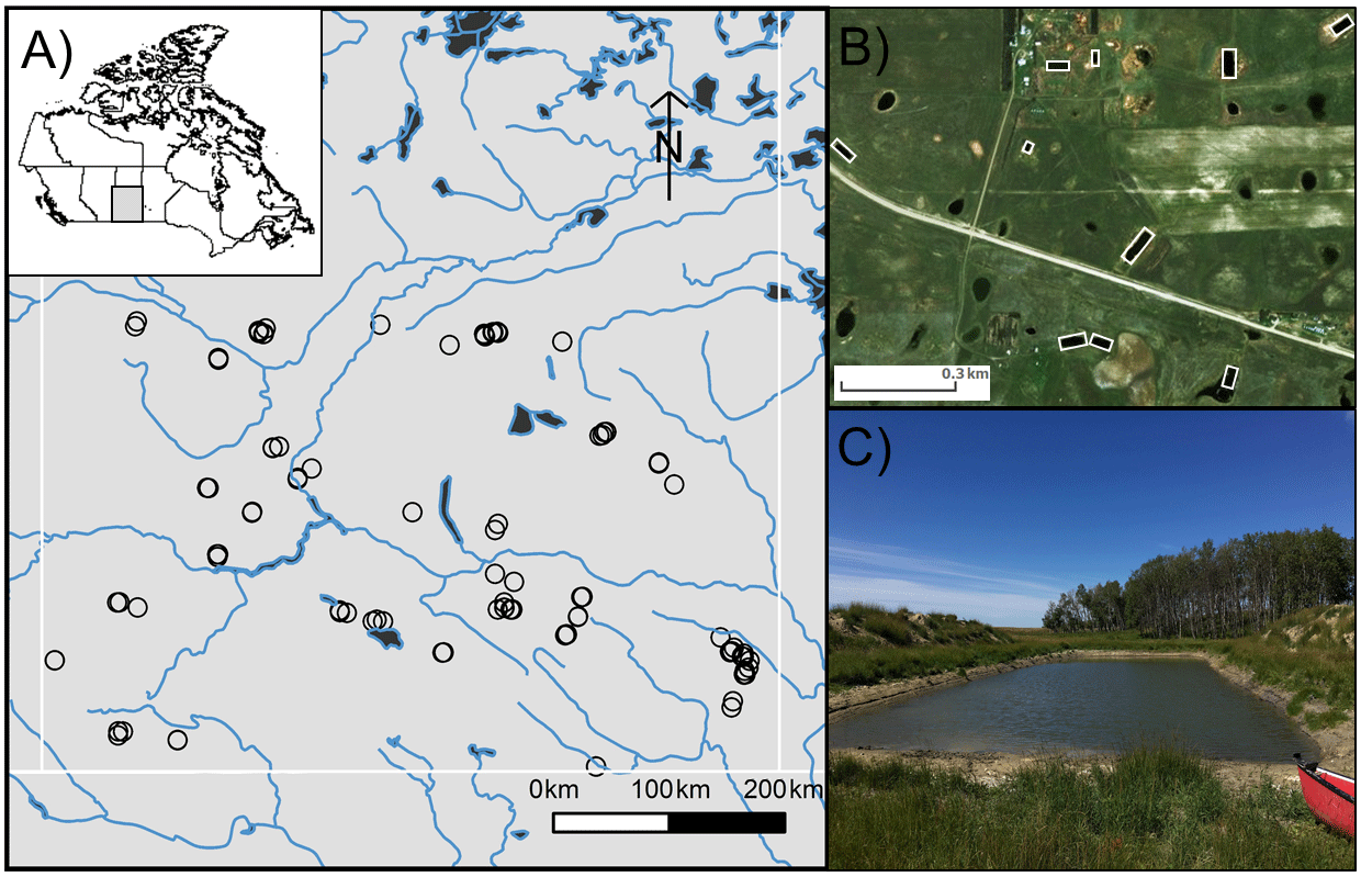
Figure 1(a) Map of southern Saskatchewan in Canada showing the distribution of studied farm reservoirs, (b) aerial image showing 10 farm reservoirs delineated by white rectangles within a 1 km² area, and (c) general size and shape of farm reservoirs with two characteristic side mounds of excavated materials.

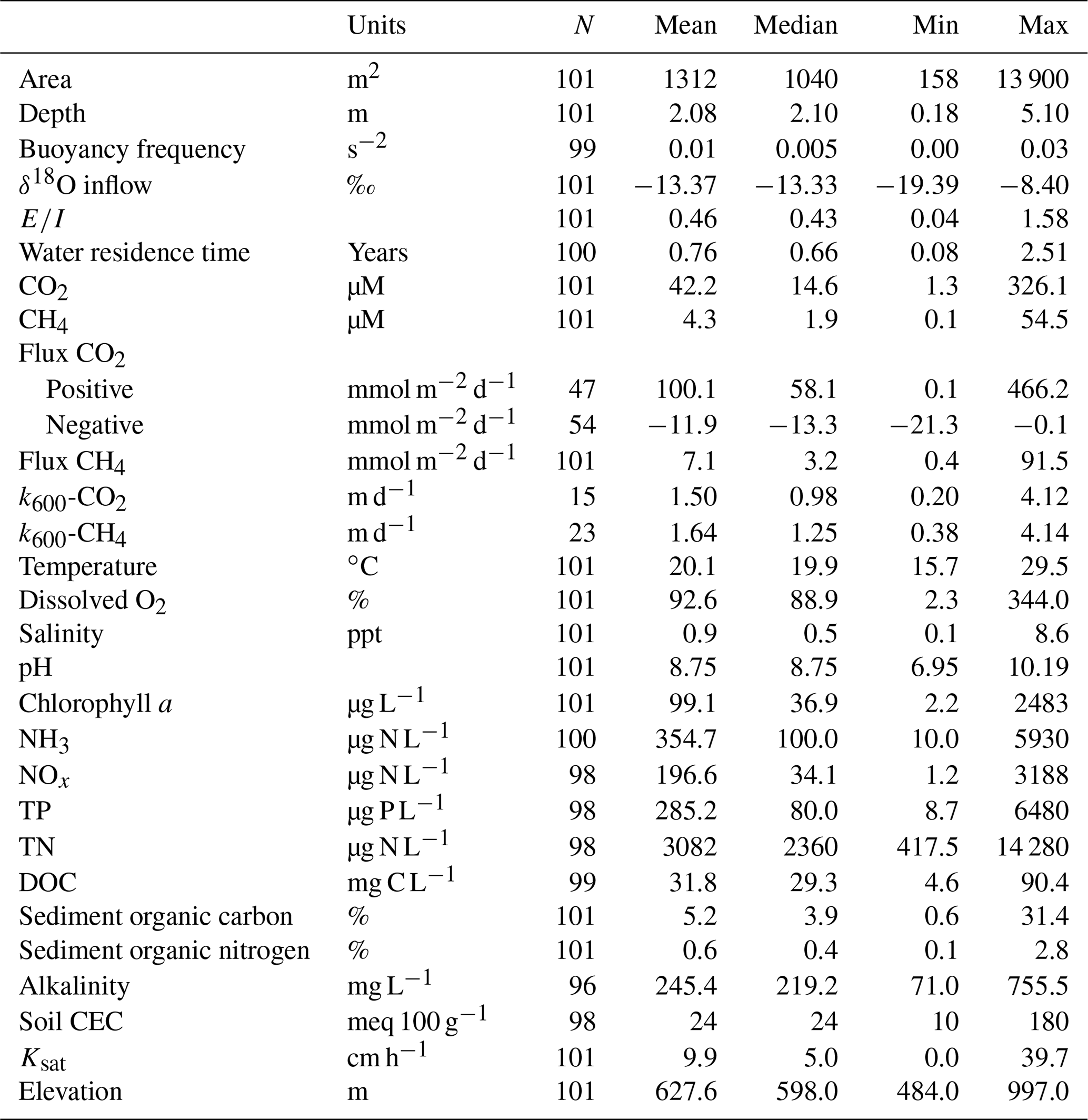
Small farm reservoirs (known locally as “dugouts”) are a prominent feature of the landscape, with densities of up to 10 km⁻² (Fig. 1b). Up until 1985, over 110 000 farm reservoirs had been constructed in Saskatchewan (Gan, 2000), although subsequent densities are unknown. We sampled 101 farm reservoirs between July and August 2017, ranging in surface area from 158 to 13 900 m² (Table 1), including basins in pasture (n=18), pastures with livestock (n=62), and cropland (n=21) sites. Each site was sampled once during this period, between the daylight hours of 10:00 and 15:00 Central Standard Time (CST; or GMT−6). Saskatchewan farm reservoirs are typically uniform in shape and morphometry, dug to a depth of 4 to 6 m with steep sides (1.5 : 1 slopes). Most shallow wetlands and lakes in the region exhibit water balances dominated by evaporation and limited inflow from winter precipitation or groundwater (Conly and van der Kamp, 2001; Pham et al., 2009). Farm reservoirs differ from small natural waterbodies in that they have a higher ratio of water volume to surface area, designed to minimize evaporation losses. Despite this feature, arid conditions persisted during the sampling year, with reduced (34 %–65 %) annual rainfall such that many reservoirs were only half their designed depth. Natural waterbodies also tend to be high-pH hard-water systems, owing to the soils which consist of glacial till high in carbonates (Last and Ginn, 2005). The same was observed for the majority of farm reservoirs, with an average pH of 8.75 (Table 1).

Table 1Farm reservoir and landscape physical, hydrological, and chemical characteristics of the study sites (n=101).

Download Print Version | Download XLSX

2.2 CO₂ and CH₄ measurements

Dissolved gas samples were collected using the in-field headspace extraction method (Webb et al., 2019). Briefly, water was collected from ∼30 cm below the surface using a submersible pump which filled a 1.2 L glass-serum bottle, ensuring the bottle overflowed and no air bubbles were present. The bottle was sealed with a rubber stopper fitted with two three-way stopcock valves. Using two 60 mL airtight syringes, atmospheric air was added to the bottle whilst simultaneously extracting 60 mL of water. The bottle was then shaken for 2 min to ensure gas equilibration in the headspace. Two analytical replicates were extracted and stored in 12 mL evacuated Exetainer vials with double-wadded caps. Headspace concentrations of CO₂ and CH₄ were measured using gas chromatography with a Scion 456 gas chromatograph (Bruker Ltd.) and calculated using standard curves. Dry molar fractions were corrected for dilution and converted to concentrations according to solubility coefficients (Weiss, 1974; Yamamoto et al., 1976).

To compare with the literature and assess the source/sink behaviour of the reservoirs, diffusive fluxes of carbon dioxide and methane fluxes were estimated for each waterbody. Given that the focus of the study was to investigate drivers of CO₂ and CH₄ concentrations across farm reservoirs, ebullition events were not measured during this survey and as such total CH₄ fluxes are likely underestimated. Diffusive fluxes were estimated using water-column concentrations (C_water) and average farm reservoir gas transfer velocity (k_c) using the following equation:

where f_C is the flux of CO₂ or CH₄ (mmol m⁻² d⁻¹) and C_air is the ambient air concentration. The average global mixing ratios for the sampling period of 406 and 1.85 µatm were used for ambient concentrations for CO₂ and CH₄, respectively (Mauna Loa NOAA station, June to August 2017). Site-specific gas transfer velocity (k_c) was determined from 30 individual floating-chamber (area = 0.23 m², volume = 0.046 m³) measurements carried out on a subset of 10 reservoirs. During each 10 min deployment, changes in gas concentrations were measured at 2.5 min intervals by taking samples using syringes and dispensing gases into pre-evacuated 12 mL vials. The flux (mmol m⁻² d⁻¹) was calculated from the observed rate of change in the dry mole fraction of the respective gas (Lorke et al., 2015). The gas transfer velocity normalized to a Schmidt number of 600 (k₆₀₀) for each respective gas was then determined using measured flux, in situ gas concentrations, atmospheric concentration, Henry's constant, and Schmidt numbers, assuming a Schmidt exponent of 0.67. The average k₆₀₀ calculated from the floating-chamber deployments was 1.50±1.34 and 1.64±1.14 m d⁻¹ for CO₂ and CH₄, respectively (Table 1).

For comparing CO₂-equivalent fluxes, CH₄ fluxes were converted using the 100-year sustained-flux global warming potential (SGWP, Neubauer and Megonigal, 2015). This metric offers a more attainable measure of ecosystem climatic forcing, assuming gas flux persists over time instead of occurring as a single pulse as quantified using traditional global warming potentials (GWP, Myhre et al., 2013). Here, a SGWP multiplier of 45 was applied to all CH₄ fluxes in the literature comparison, which is slightly higher than the traditional GWP of 32 over a 100-year time frame (Myhre et al., 2013).

2.3 Abiotic and biotic variables

A range of abiotic and biotic parameters were measured at each site. Water quality variables including temperature (^∘C), pH, dissolved O₂ (DO; % saturation), conductivity (µS cm⁻²), and salinity were measured at 0.5 m intervals from the surface to the bottom using a YSI (Yellow Springs Instruments, OH, USA) multi-probe meter. Surface (0.5 m) samples for water chemistry were collected using a submersible pump. Upon collection, samples for dissolved nitrogen (NO₃+NO₂, NH₄, total dissolved N; µg N L⁻¹), soluble reactive phosphorus (SRP; µg P L⁻¹) and total dissolved P (TDP; µg P L⁻¹), dissolved organic and inorganic carbon (DOC, DIC; mg C L⁻¹), alkalinity ($\mathrm{OH}+{\mathrm{HCO}}_{\mathrm{3}}+{\mathrm{CO}}_{\mathrm{3}}$; mg L⁻¹ as CaCO₃), and water isotopes (δ²H, δ¹⁸O; ‰) were filtered through a 0.45 µm pore membrane filter. Nutrient and dissolved carbon samples were stored in a dark bottle at 4 ^∘C until analysis. Chlorophyll a (Chl a) samples were collected on GF/C glass-fibre filters (nominal pore size 1.2 µm) and frozen (−10 ^∘C) until analysis. Sediment samples were collected at the centre of each reservoir, with the uppermost 10 cm using an Ekman grab sampler, and were frozen at −10 ^∘C until analysis.

Most analyses were carried out at the University of Regina Institute of Environmental Change and Society (IECS). Water nutrient and dissolved carbon concentrations were measured on a Lachat QuikChem 8500 and Shimadzu model 5000A total carbon analyzer, following standard analytical procedures, respectively (Patoine et al., 2006; Finlay et al., 2009). Alkalinity was measured using standard methods of the US Environmental Protection Agency (EPA) on a SmartChem 200 Discrete Analyzer (WestCo) and estimated as the concentration of CaCO₃ (EPA, 1974). Chl a was analysed using standard trichromatic methods (Finlay et al., 2009). The total carbon and nitrogen content (% dry weight) of freeze-dried sediment samples were determined on a NC2500 Elemental Analyzer (ThermoQuest, CE Instruments).

2.4 Hydromorphology

Morphometric parameters of reservoirs were estimated for each site. The depth of each farm reservoir was measured during using a portable ultrasonic depth sounder, taken at the deepest section in the centre of the reservoir. Surface area was determined using Google Earth satellite imagery. Reservoir volume was calculated using the formula for a prismoid by assuming that all sites maintained their original shape, including slopes of 1.5 : 1 ratio (Andresen et al., 2015). From these measurements, an Index of Basin Permanence (IBP) was calculated (Kerekes, 1977).

The degree of water-column mixing or vertical stratification was determined by calculating the squared Brunt–Väisälä buoyancy frequency (N², s⁻²). The strongest density gradient was calculated based on vertical temperature measurements at 0.5 m depth intervals using the package rLakeAnalyzer (Read et al., 2012) in R (version 3.5.2; R Core Team, 2018).

The hydrology of farm reservoirs was estimated through analysis of δ¹⁸O and δ²H isotope values of water. Samples were collected from 0.5 m below the surface, filtered (0.45 µm pore) and stored in amber borosilicate jars at 4 ^∘C until analysis using a Picarro L2120-I cavity ring-down spectrometer (CRDS). Hydrological parameters, including evaporation-to-inflow ratio (E∕I), residence time (years), and inflow volume (m³), deuterium (²H) excess (d-excess), and δ¹⁸O inflow (δ_I) values, were calculated using the coupled isotope tracer method (Yi et al., 2008) and conventional isotopic water-balance methods (Gibson et al., 2001). All methods assumed that reservoirs were headwater systems in a hydrological steady state (Yi et al., 2008). Model inputs included information about the local meteoric water line (LMWL), the trajectory of evaporation along a local evaporative line (LEL), and regional meteorological conditions. From here, the water mass balance of a given waterbody can be quantified based on its relative position along the LEL (Gibson et al., 2001).

Briefly, the isotopic inflow values were estimated by the intercept between the LMWL and site-specific LEL as determined by the δ¹⁸O evaporation value (δ_E) and δ¹⁸O reservoir water value at each site (Yi et al., 2008). The E∕I ratio was calculated by using headwater isotopic models of the water mass balance ($({\mathit{\delta }}_I-{\mathit{\delta }}_L)\cdot ({\mathit{\delta }}_E-{\mathit{\delta }}_L{)}^{-\mathrm{1}}$). Hydrologic residence time was estimated from the reservoir volume and the water isotopic values of waterbodies, inflow, and evaporation. Deuterium excess (d-excess ‰ = ${\mathit{\delta }}^{\mathrm{2}}\mathrm{H}-\mathrm{8}\cdot {\mathit{\delta }}^{\mathrm{18}}\mathrm{O}$) was calculated as an additional indicator of evaporation losses, where lower values ($<-\mathrm{10}$ ‰) indicate isotopic enrichment from precipitation (Brooks et al., 2014).

2.5 Landscape properties

Landscape soil data were obtained from the National Soil DataBase, Government of Canada (http://sis.agr.gc.ca/cansis/nsdb/dss/v3/index.html, last access: 31 October 2019), using ArcGIS to extract the soil attributes at each site. Extracted variables included soil salinity; soil pH; soil organic carbon content; saturated hydraulic conductivity (K_sat); cation exchange capacity (CEC); and the total composition of soil from sand, silt, and clay fractions (%). Reservoir elevation (m a.s.l.) was determined using ArcGIS and the Canadian Digital Elevation Model (CDEM, v1.1). Local land use in the immediate area surrounding each reservoir was categorized into three types based on local observations at the time of sampling. Categories included pasture land used for either livestock grazing or hay harvesting, pasture where livestock have direct access to the waterbody, and crop fields.

2.6 Statistical analyses

Environmental variables were selected based on known or presumed influence on CO₂ and CH₄ concentrations in lakes and small waterbodies. Both biotic and abiotic predictors that influence production or consumption of CO₂ and CH₄ were selected, including DO, alkalinity, NO_x (NO₂+NO₃), NH₄, dissolved inorganic nitrogen (DIN), total dissolved nitrogen (TDN), TDP, Chl a, DOC, conductivity, pH, and sediment organic C:N ratio. The influence of reservoir hydrology and morphology was also examined, including measures of surface area, basin permanence, hydrologic regime (E∕I), water source (δ_I), and degree of mixing (or stratification). Finally, potential effects of the surrounding terrestrial landscape were estimated in models using soil properties, elevation, and land use practises to account for any localized landscape drivers. Before testing relationships, all predictors were transformed as needed using either log₁₀ or square root to remove skewness.

The relationships between covariates and CO₂ and CH₄ were estimated using generalized additive models (GAMs). GAMs provide an ideal approach to model non-linear associations between predictor variables and responses, using the sum of unspecified smooth functions to estimate trends. GAMs are not constrained by prescribed assumptions associated with parametric models such as linearity of link-scale effects in generalized linear models. Instead, the functional form of the partial relationships between covariates and the response is determined from the data. The more flexible modelling approach is useful where the effects of covariates on the response are non-linear and has been applied to complex aquatic datasets assessing GHGs (Wiik et al., 2018; Webb et al., 2019). GAMs were developed with a gamma distribution for the response and the log link function. Each model included covariates that represented hydromorphological, abiotic and biotic, and landscape controls. To avoid multicollinearity, correlation coefficients and statistical significance (p<0.05) between pairs from Pearson linear correlation tests were used to guide covariate choice before model fitting (Tables S1–S3 in the Supplement). Candidate variables were then selected for each model to test which variables best estimate variability in CO₂ and CH₄ concentrations. All model coefficients were estimated using restricted marginal likelihood with the mgcv package (Wood, 2011; Wood et al., 2016) for R (version 3.5.2; R Core Team, 2018).

3.1 Models

Regional variation in CO₂ concentrations were best estimated in a GAM including pH alone, with 86.3 % of deviance explained and a strongly declining CO₂ at pH above 8 (Fig. S1 in the Supplement). Exclusive of the model with pH, the detailed mechanistic GAM for estimating CO₂ concentrations across farm reservoirs included a combination of DO saturation, alkalinity, NO_x, thermal stratification (buoyancy frequency), basin hydrology (the interaction between δ_I and WRT), and landscape features (soil CEC, elevation, soil salinity) (Fig. 3). Overall, the model explained 66.5 % of deviance in CO₂ concentrations (Table S4, Fig. S2). All covariates had a significant effect except soil salinity, with DO, alkalinity, and the interaction between δ_I and WRT being the strongest predictors (p<0.001). CO₂ concentrations displayed a positive response with increasing alkalinity, NO_x, buoyancy frequency, and soil CEC, with a generally negative response to increasing DO and elevation. The effect of DO on CO₂ was particularly distinct between 25 %–100 % O₂ saturation (Fig. 3a). The interactive effect of hydrology parameters suggests that sites with elevated rain inflows (${\mathit{\delta }}^{\mathrm{18}}\mathrm{O}>-\mathrm{12.5}$ ‰) and longer WRT will exhibit undersaturated CO₂ concentrations.

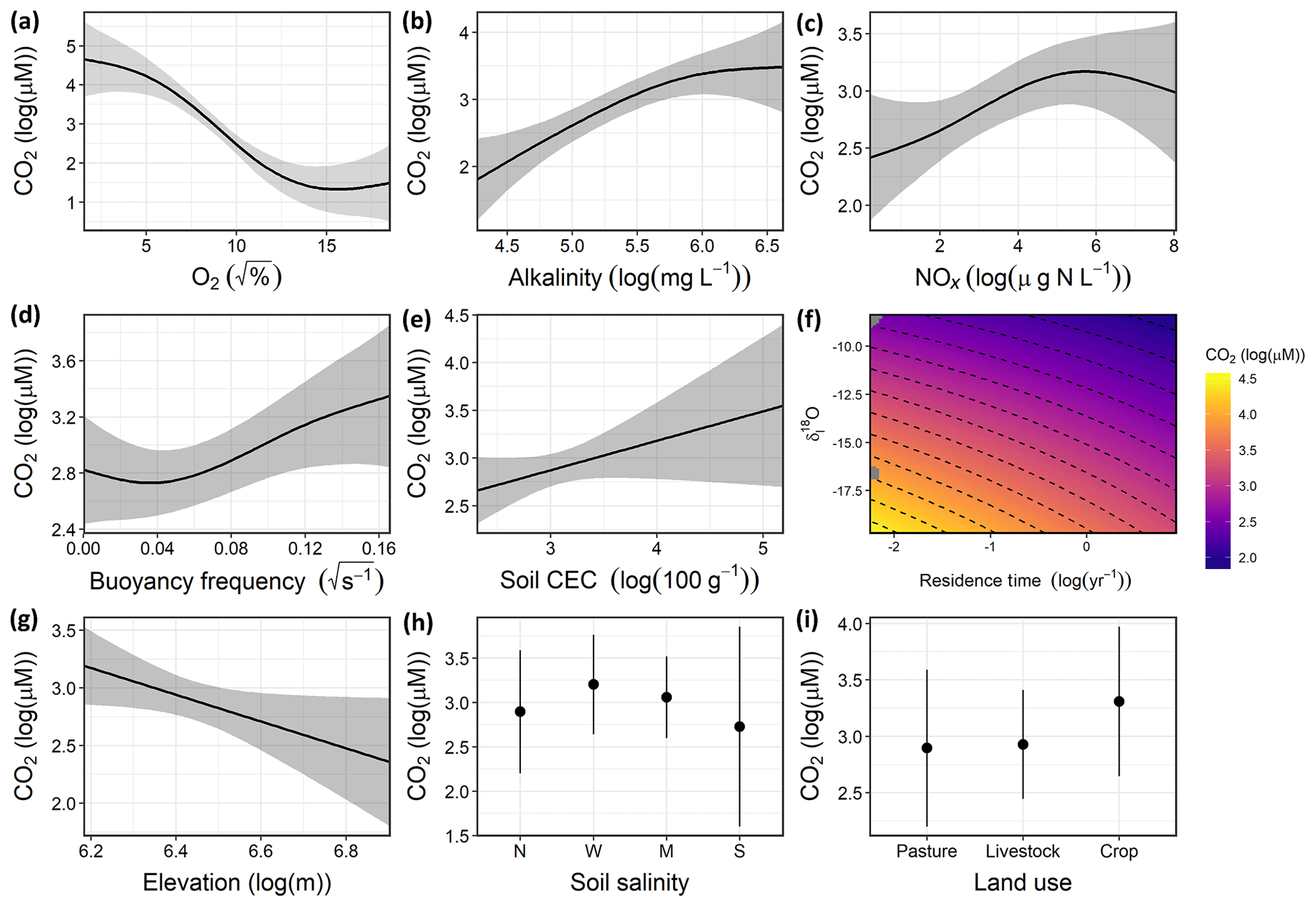
Figure 3Response patterns of farm reservoir CO₂ concentrations with abiotic, biotic, hydromorphological, and landscape variables based on GAMs. CO₂ was best estimated by a combination of (a) DO saturation, (b) alkalinity, (c) NO_x, (d) buoyancy frequency, (e) interaction between δ_I and WRT, (f) soil CEC, (g) and elevation, with soil salinity (non-saline, N; weakly saline, W; moderately saline, M; strongly saline, S) (h) and land use (i) not significant. Model deviance explained was 66.5 %. The response patterns shown are the partial effect splines from the GAM (solid line), and the shaded area indicates 95 % credible intervals. See Table S4 and Fig. S2 for summary of model statistics and model fit with observed data.

Download

Variation in CH₄ concentrations among waterbodies was explained by a combination of DO saturation, sediment C∕N ratio, DIN, conductivity, the interaction between δ_I and WRT, and local land use (Fig. 4), with buoyancy frequency, soil K_sat, and elevation not significant. Overall, the GAM explained 74.1 % of the deviance in CH₄ (Table S5, Fig. S3). Concentrations of CH₄ increased with sediment C∕N and DIN and decreased with conductivity. The significant unimodal relationship with DO indicates that the highest observed CH₄ concentrations occurred under both anoxic and supersaturated O₂ environments (Fig. 4a), while low CH₄ levels were seen when inflow was more composed of snowmelt or groundwater (depleted isotope values) and WRT was long (Fig. 4f). In contrast to the CO₂ model, soil properties and elevation were not significant drivers, yet local land use was significant, with crop sites having significantly higher CH₄ compared to pastures.

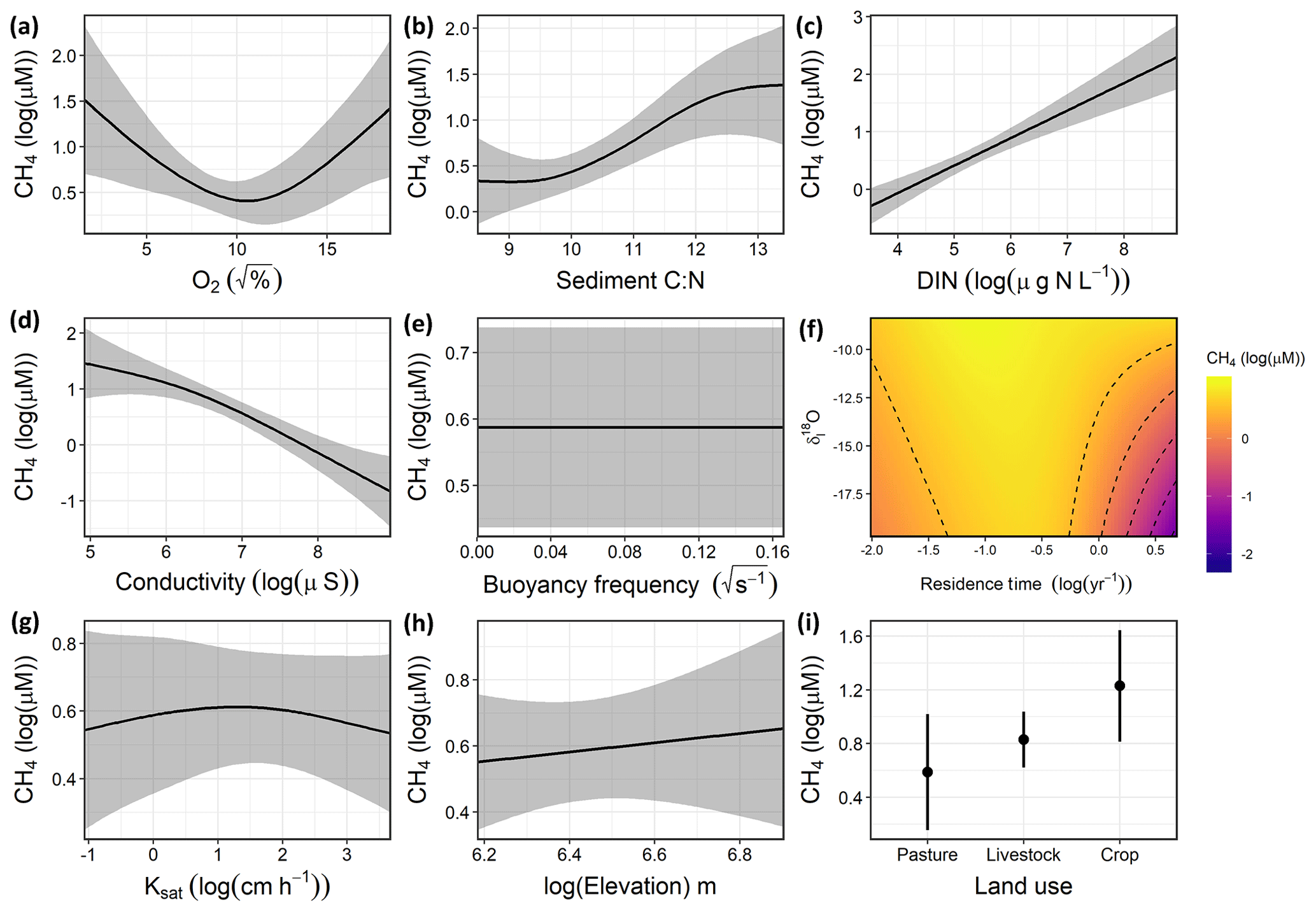
Figure 4Response patterns of farm reservoir CH₄ concentrations with abiotic, biotic, hydromorphological, and landscape variables based on generalized additive models (GAMs). CH₄ was explained by a combination of (a) DO saturation, (b) sediment C∕N, (c) DIN, (d) conductivity, (e) buoyancy frequency (not significant), (f) interaction between δ_I and WRT, (g) soil K_sat (not significant), (h) elevation (not significant), and (i) local land use. Model deviance explained was 74.1 %. The response patterns shown are the partial effect splines from the GAM (solid line), and the shaded area indicates 95 % credible intervals. See Table S5 and Fig. S3 for summary of model statistics and model fit with observed data.

Download

4.1 Environmental drivers of CO₂ concentrations

As seen in other hard-water ecosystems, variations in CO₂ were strongly coupled to differences among sites in water-column pH (Finlay et al., 2015; Müller et al., 2016). We demonstrate this relation with the strong correlation observed between CO₂ and pH in a separate GAM of only water pH as a covariate, explaining 86.3 % of deviance (Fig. S1). As expected, the role of pH in regulating CO₂ content is most pronounced at values between 8.6 and 9.0, the transition point where the predominant species of DIC shifts from free CO₂ to ${\mathrm{HCO}}_{\mathrm{3}}^{-}$ (Duarte et al., 2008; Finlay et al., 2015). Above this value, carbonate buffering increasingly regulates pH and restricts CO₂ to only trace fractions of total DIC (Stumm and Morgan, 1970). However, direct changes in CO₂ concentrations can also alter water-column pH, such as biological metabolism (Talling, 2010). Therefore, given the direct chemical relationship between pH and CO₂ concentrations (Stumm and Morgan, 1970), we opted to leave pH out of our model to further investigate the underlying biological, chemical, hydrological, and land use mechanisms.

The detailed GAM showed that variance in CO₂ concentrations among farm reservoirs was estimated (66.5 % of deviance) by a combination of predictors related to water-column productivity and microbial metabolism (DO saturation, alkalinity, NO_x), thermal stratification (buoyancy frequency), basin hydrology (the interaction between δ_I and WRT), and landscape features (soil CEC, elevation) (Fig. 3) but not local soil salinity. This pattern was shown by the DO, alkalinity, δ_I, and WRT covariates having the most significant effect at p<0.001, while CO₂ concentrations did not vary significantly between different soil salinity levels (Table S4, Fig. 3).

Carbon dioxide and dissolved oxygen are closely linked by biological metabolism in aquatic systems and diverge when other chemical or physical processes occur. Here, we see evidence for both linked and divergent processes (Fig. 3a). The tight linear relationship between CO₂ and O₂ at 25 % to 100 % saturation indicates close coupling between the gases. This likely represents control via metabolic processes such as net ecosystem production (NEP) or chemical oxidation of reduced species (Stets et al., 2017). In contrast, relationships between CO₂ and O₂ were less well defined a both high and low oxygen saturations, conditions which may indicate a greater contribution from anaerobic production of CO₂ (Torgersen and Branco, 2008; Holgerson, 2015). Alternatively, alkalinity buffering can mediate the effect of NEP on CO₂ concentrations at both extreme ranges of the DO spectrum (Marcé et al., 2015). Alkalinity buffering is most likely to affect CO₂–DO relationships in waters where alkalinity is >2000 µeq L⁻¹ (Stets et al., 2017), which was the case for ∼90 % of our sites (Table 1; Fig. 3).

Stratification can also weaken the impact of DO as a driver for CO₂ by regulating the effect of sediment respiration on epilimnetic chemistry (Huotari et al., 2009; Holgerson, 2015). Our model shows that those sites that were most stratified (elevated buoyancy frequency) exhibited higher CO₂ concentrations (Fig. 3d). This pattern contrasts those observed in other small lentic systems where elevated epilimnetic CO₂ concentrations were observed during and after the breakdown of water-column stratification (Huotari et al., 2009; Glaz et al., 2016). Preliminary seasonal studies of some farm reservoirs in 2018 show that stratification is strong and persistent throughout the summer, with no obvious diurnal mixing events. Such strong stratification can maintain anoxic conditions throughout most of the water column, which supports intense anaerobic respiration and CO₂ production.

The positive association between NO_x and CO₂ found in our reservoirs is consistent with similar patterns seen with dissolved inorganic N species in other artificial waterbodies (Ollivier et al., 2019; Peacock et al., 2019) and regional prairie lakes (Wiik et al., 2018). In some lakes, high N loading favoured elevated heterotrophy, despite simultaneous boosts in primary production, which draw down free CO₂ (Huttunen et al., 2003; Cole et al., 2000). The effect of a high N influx on CO₂ may be heightened in smaller or shallow lentic waters which are more influenced by sedimentary processes (Torgersen and Branco, 2008). Further, high N availability can increase algal biomass and the deposition of fresh organic matter (OM) made increasingly available for bacterial respiration (Cole et al., 2000). As a result, the effect of increased benthic respiration offsets CO₂ uptake by primary producers, while extremely high influx of dissolved N can also favour microbial processes such as denitrification which increase CO₂ evolution (Bogard et al., 2017).

Hydrological controls were found to be important regulators of CO₂ concentrations in these farm reservoirs. Sites which received most of their inflow from snowmelt or groundwater, and which had short WRT, supported supersaturated CO₂ concentrations (Fig. 3f). Such patterns may reflect increased inputs of groundwater which are typically supersaturated with CO₂ (Macpherson, 2009). Long WRT is associated with larger, deeper systems. These sites are usually less influenced by the terrestrial–aquatic interface, take longer to concentrate the effect of any catchment-derived solutes (Junger et al., 2019), and have higher biotic assimilation of nutrients (Devito and Dillon, 1993; Fairchild and Velinsky, 2006). Larger waterbodies may also be able to better mediate stream or groundwater C inputs through longer chemical processing times and transformations. For example, agricultural reservoirs with the highest WRTs tended to be hydrologically closed systems ($E/I>\mathrm{1}$) and any watershed-derived DIC delivered from previous water sources is likely to be consumed by primary production, which encourages atmospheric CO₂ uptake (Macrae et al., 2004). Additionally, smaller waterbodies with shorter WRT can support higher rates of internal CO₂ production due to higher rates of allochthonous DOC mineralization (Weyhenmeyer et al., 2015; Vachon et al., 2017).

Groundwater delivery of DIC-rich porewater is the most likely hydrological source resulting in CO₂ enrichment of small farm reservoirs. This mechanism is also suggested by the observation that higher reservoir CO₂ concentrations are predicted in high-CEC soils. Alkaline high-CEC soils retain more calcium ions within clay particles, which releases carbonates and bicarbonates into soil porewater (Kelley and Brown, 1934). Although regional snowmelt and groundwater have similar isotopic signatures (Pham et al., 2009; Jasechko et al., 2017), the positive correlation of CO₂ with alkalinity suggests groundwater as the main source. Edaphic sources of inorganic carbon can result in farm waterbodies accumulating dissolved CO₂, bicarbonates, and carbonates, and therefore alkalinity, from the surrounding soils via groundwater discharge (Miller et al., 1985). Other studies have found strong evidence for groundwater inputs driving CO₂ supersaturation in small lentic systems (Perkins et al., 2015; Peacock et al., 2019) and watershed-derived alkalinity driving CO₂ supersaturation in lakes (Marcé et al., 2015).

Finally, landscape elevation had a significant external effect on reservoir CO₂ and may represent diverse weak controls related to landscape setting. Lower CO₂ concentrations at higher elevations are common in perched ecosystems with smaller contributing catchment areas (Diem et al., 2012) and low rates of allochthonous carbon influx (Rose et al., 2015). Conversely, waterbodies low in the landscape may receive more watershed C via groundwater influx due to topographical gradient (Winter and LaBaugh, 2003; van der Kamp and Hayashi, 2009). The effect of elevation could also be related to changes in vegetation composition within the local landscape, with the lowest lying catchments exhibiting higher abundance of marginal wetland vegetation (Zhang et al., 2010), which favours higher inputs of terrestrial C (Magnuson et al., 2006; Abril et al., 2014).

4.2 Environmental drivers of CH₄ concentrations

The GAM suggested that CH₄ concentrations were primarily related to internal biogeochemical processes and the influence of the hydrological regime. For example, factors related to water-column productivity (DO, sediment C∕N, DIN, conductivity) had the most significant effect (p<0.01), while some of the broader landscape features such as soil K_sat and elevation had no significant effect on CH₄ levels. The nutrient status of waterbodies is often a primary driver of high CH₄ emissions in lakes, impoundments, and ponds (Deemer et al., 2016; Beaulieu et al., 2019; Peacock et al., 2019). Consequently, high nutrient availability is likely fuelling elevated values in both O₂ saturation and CH₄ (Fig. 4a). High CH₄ concentrations at low O₂ saturation reflect the development of anoxic habitats which favour methanogenesis (Huttunen et al., 2003; Bastviken et al., 2004). This is likely the result of rapid biomass production which both enriches epilimnion with O₂ and depletes O₂ in the hypolimnion by providing fresh labile organic matter for decomposition.

In support of eutrophication-driven CH₄ production, our model indicated that high proportions of autochthonous organic matter in sediments were associated with elevated concentrations of CH₄ (Fig. 4b). Overall, sedimentary C∕N ratios were in the range (8.5 to 13.4) expected for both phytoplankton and submerged macrophytes (Liu et al., 2018). This suggests that in situ rather than terrestrial organic matter was likely the main source of C fuelling methanogenesis in these reservoirs, although increasing CH₄ concentrations with C∕N may also represent a larger contribution of terrestrial OM. Strong associations of labile autochthonous C and CH₄ production in sediments (Due et al., 2010; Crowe et al., 2011) also suggests a direct link between eutrophication and CH₄ production in small farm waterbodies.

Thermal stratification of the water column did not significantly influence surface CH₄ concentrations in small farm reservoirs (Fig. 4e). This finding contrasts with observations from other small waterbodies where limited mixing favours CH₄ accumulation (Kankaala et al., 2013). Although some small systems exhibit diurnal mixing patterns with turnover at night (Glaz et al., 2016), the wide range of buoyancy frequency values (0.00 to 0.16) suggests that at least some farm reservoirs are continuously stratified, particularly in deeper ponds (Kankaala et al., 2013), as noted for CO₂ distributions (see above and Fig. 3d). Taken together, our findings suggest that variability in the biological production of CH₄ likely exerts a stronger influence over CH₄ concentrations across farm reservoirs than does physical mixing, and this further supports the hypothesis that the prevailing sediment and water chemistry are the primary controls of CH₄ concentrations.

Although the hydrological regime of small water bodies is rarely measured, we find that water source (rain, snow/groundwater) and reservoir retention time interact to influence CH₄ concentrations (Fig. 4f). In particular, CH₄ concentrations were lowest when WRT was long (>1 year) and water was derived mainly from snow or groundwater sources (δ¹⁸O depleted). This may be due to a combination of reasons, including the prevalence of sulfate delivered from groundwater (Pennock et al., 2010), dilution of waterbody from snowmelt inflow, and sediments depleted in labile carbon due to longer biogeochemical processing times in the dams. The potential effect of sulfate limiting methanogenesis is in agreement with the strong negative relationship found between CH₄ and conductivity in our model (Fig. 4d). Sulfate makes up a large portion of the ionic composition of groundwater in the Prairie Pothole Region due to pyrite oxidation (Goldhaber et al., 2014). Evidently, the biological influence on CH₄ concentrations appears less pronounced in these larger, low-flow dams.

In contrast to the external drivers found for CO₂, local land use had a significant effect on CH₄ concentrations in farm reservoirs (Fig. 4i), with significantly higher CH₄ levels in cropland waterbodies than those in pasture. Catchment land use regulates the physico-chemical properties of ponds (Novikmec et al., 2016) by influencing the degree of local vegetative cover and associated influx of allochthonous C to waterbodies (Whitfield et al., 2011). Similarly, regions with crops undergo more intensive agricultural modification, with fertilization, crop rotations, and mechanical disturbance of soil, which all lead to greater nutrient runoff and soil erosion. Our finding contrasts with those from Australian farm reservoirs where diffusive CH₄ fluxes were 250 % higher in reservoirs with livestock compared to crops, although the mechanisms responsible for observed differences were inconclusive (Ollivier et al., 2019). This difference could be the result of the intensity of agricultural production, where farm reservoirs supporting high intensity grazing may also experience high CH₄ production as demonstrated by a couple of high CH₄ concentrations observed in our livestock pasture reservoirs (Fig. 2). In this case it is likely that CH₄ levels are more influenced by nutrient loading from the landscape which stimulates eutrophication (Huttunen et al., 2003), as suggested by the biotic variables in our model (Fig. 4). The intensity of agricultural production under different land use types should be an area of further exploration for external controls on farm reservoir GHG production.

4.3 Emissions from farm reservoirs compared to other small waterbodies

To date, small waterbodies on farms have been shown to be large emitters of both CO₂ and CH₄ (Fig. 5). However, in our study we show that this is not always the case. Diffusive fluxes varied −21 to 466 and 0.14 to 92 mmol m⁻² d⁻¹ for CO₂ and CH₄, respectively. These findings are consistent with other small artificial waterbodies which are strong CH₄ sources that exhibit a large range of variability from 0.02 to 33 mmol m⁻² d⁻¹ (Grinham et al., 2018a; Ollivier et al., 2019). Average CH₄ fluxes from our farm reservoirs correspond to 417 kg CH₄ ha⁻¹ yr⁻¹, which is greater than the current IPCC emission factor estimate of 183 kg CH₄ ha⁻¹ yr⁻¹ (IPCC, 2019). Considering the skewness of our CH₄ data, our median value of 184 kg CH₄ ha⁻¹ yr⁻¹ agrees with the emission factor of other artificial ponds.

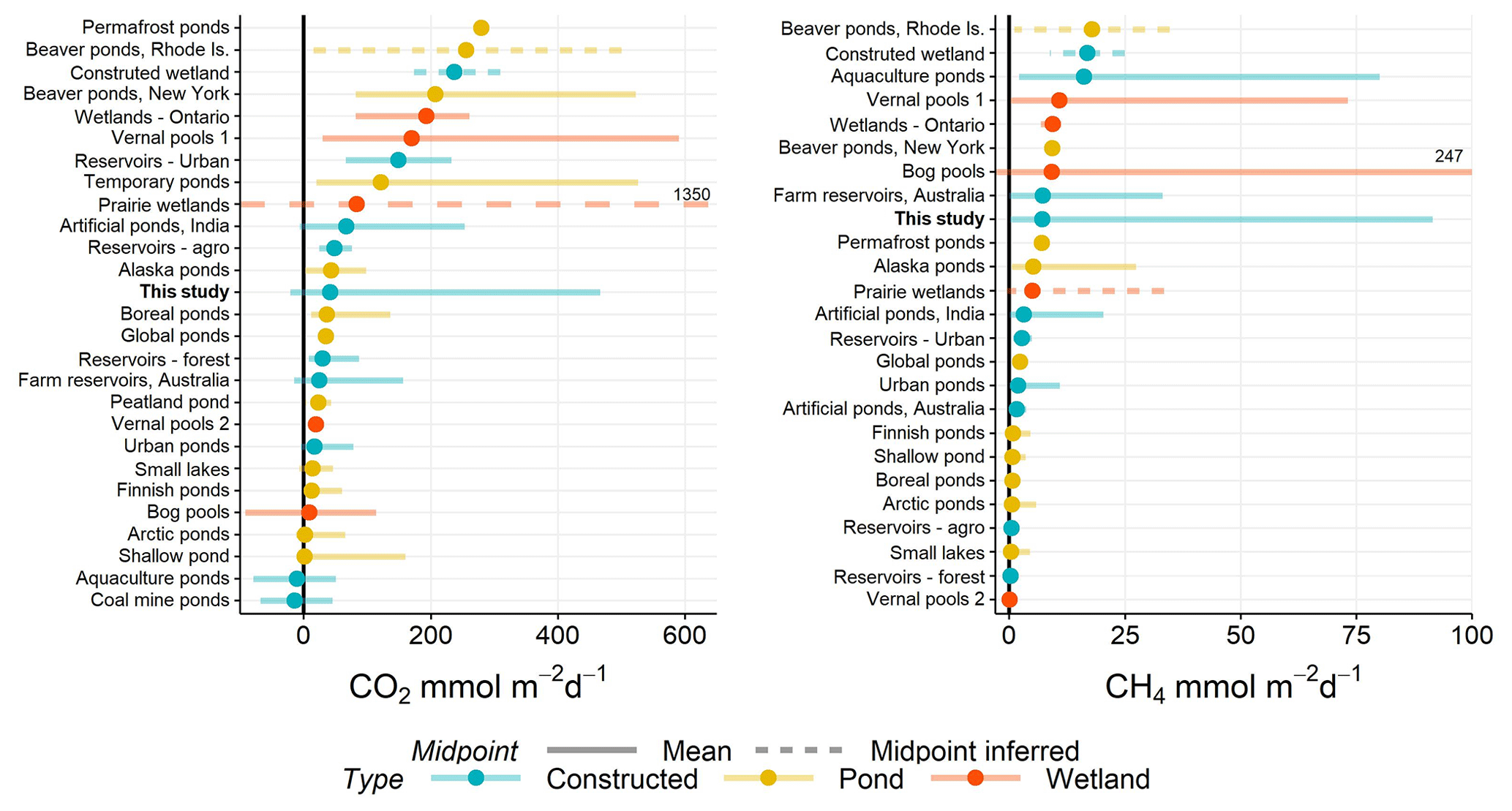
Figure 5Range of CO₂ and CH₄ (diffusive) fluxes observed in natural and constructed small (<0.01 km²) waterbodies, including this study (farm reservoirs). Dots represent the mean reported in each study and error bars the range. If no mean value was reported, then the midpoint was inferred as the middle of range (dashed lines). Solid black line distinguished between positive and negative fluxes. All data are from the published literature and references can be found in the Table S6.

Download

The negative fluxes observed in our farm dams represents one of the few studied small waterbodies that exhibit CO₂ sink behaviour, with most showing net heterotrophy (Fig. 5). Although other studies have noted CO₂ sink behaviour in artificial ponds and reservoirs (Peacock et al., 2019; Ollivier et al., 2019), this is the first study to capture such a high proportion (>52 %) of CO₂ uptake in such systems, with negative fluxes estimated to range between −21 and −0.1 mmol m⁻² d⁻¹ (mean −12 mmol m⁻² d⁻¹) for CO₂ (Table 1). These flux ranges compare to CO₂ uptake of −1 to −11 mmol m⁻² d⁻¹ in agricultural eutrophic lakes of North America (Finlay et al., 2010; Pacheco et al., 2014). Studies have shown the importance of eutrophication, leading to net autotrophy, in enhancing CO₂ uptake and reversing carbon fluxes in lakes (Pacheco et al., 2014). However, a global analysis of GHG fluxes from lakes and reservoirs revealed that the consequence of increased CH₄ emissions with increasing trophic status often outweighs the impact of negative CO₂ fluxes (Deemer et al., 2016). Here, our model shows the potential importance of reservoir placement within the landscape as a way of reducing CO₂ emissions via hydrological and geochemical controls without the added consequence of increased CH₄ emissions.

When CO₂ and CH₄ fluxes from small artificial waterbodies are compared with natural small waterbodies, no apparent trend exists in which group produces more or less carbon emissions (Fig. 5). Natural ponds and constructed waterbodies have a similar range in variability of mean fluxes for both gases, while wetlands exhibit some of the greatest within-study variability. Constructed waterbodies often have lower net CO₂ efflux, suggesting that these systems more often switch between net autotrophy and heterotrophy than do small natural systems. Small artificial waterbodies have disproportionately higher CO₂ and CH₄ emissions than other natural waterbodies due to the direct impact of agricultural and urban land use (Wang et al., 2017). However, analysis of the limited literature shows that is not the case. We suggest that the lack of a clear distinction between constructed and naturally occurring small water bodies arises because of geographical variation in the relative importance of the diverse factors regulating carbon metabolism (Figs. 3, 4).

When assessing the GHG impact of constructed waterbodies, it is important to consider the relative contribution to CO₂-equivalent (CO₂-e) fluxes between CO₂ and CH₄. Here, CH₄ fluxes were converted to CO₂-e fluxes using the sustained-flux global warming potential over 100 years (Neubauer and Megonigal, 2015). On average, 8 % of farm reservoirs were acting as CO₂-e sinks on the range of −0.6 to 79 g CO₂ m⁻² d⁻¹ during the time of sampling. This number offers a snapshot of the potential for farm reservoirs to act as a net CO₂-e sink, and it is important to consider how seasonal variation influences the GHG sink/source status. Preliminary data on seasonal variation in CO₂ and CH₄ concentrations from a smaller number of farm reservoirs indicate variation (represented as the standard deviation related to the mean) ranging between 20 % and 200 % and between 40 % and 200 % for CO₂ and CH₄, respectively. Here, this variation represents monthly sampling between the periods of ice melt and ice formation on water bodies in Saskatchewan. Applying the average observed seasonal variation of 78 % and 93 % to our current spatial dataset suggests that CO₂-e emissions from farm reservoirs may vary between −1.7 and 150 g CO₂ m⁻² d⁻¹, or 0 % to 44 %, as acting net CO₂-e sinks. Further study into the consistency of potential farm reservoir CO₂ sinks on the temporal scale is required to better assess the overall GHG impact.

Small natural ponds and wetlands have some of the highest CO₂-e emission rates, with particular importance of contributions from CH₄ (Fig. 6). On average our farm reservoirs had one of the highest CH₄ contribution to CO₂-e fluxes (74 %), in agreement with the one other farm reservoir study (83 %) of CH₄ contribution (Ollivier et al., 2019). This large contribution from CH₄ is similar to patterns recorded from lakes and impoundments globally, where large freshwater bodies contribute to 75 % of all CO₂-e efflux (DelSontro et al., 2018). Fortunately, because the factors that regulate CH₄ emissions are becoming better identified (Fig. 4), there exists the possibility that artificial wetlands can be constructed to minimize CH₄-related CO₂-e emissions and mitigate the overall large rate of CO₂-e emissions from agriculture (Robertson et al., 2000).

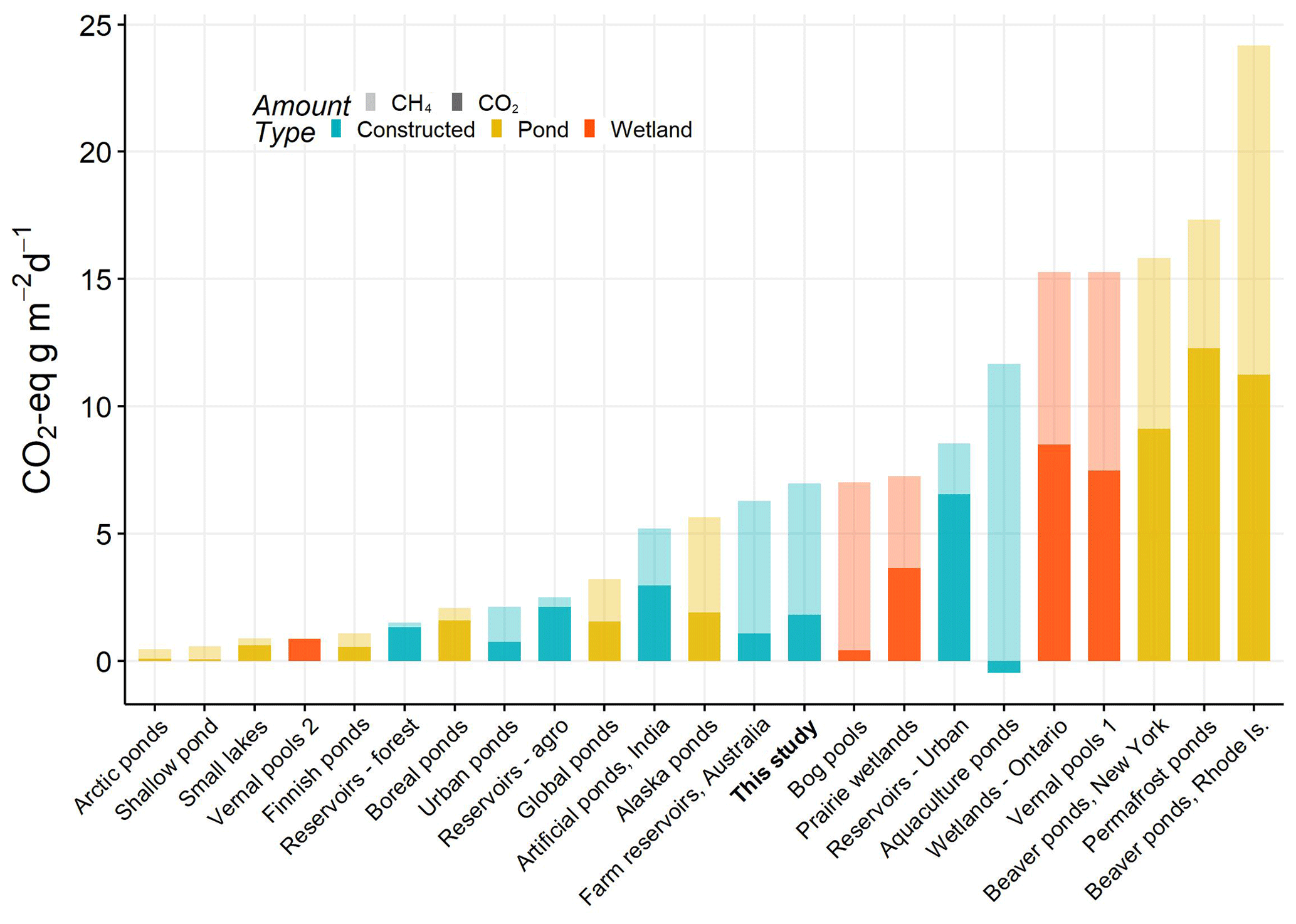
Figure 6Total average CO₂ equivalent fluxes of CO₂ and CH₄ (diffusive) measured in natural and artificial small waterbodies (<0.01 km²). CO₂-e fluxes were calculated based on 100-year sustained-flux global warming potentials in Neubauer and Megonigal (2015). Relative proportions of each gas are indicated by shading, and waterbody type is given by colour. All data are from the published literature and references can be found in the Table S6.

Download

4.4 Minimizing emissions: potential management solutions

A combination of factors, including landscape position, construction, and management, could optimize features to minimize carbon emissions from reservoirs and potentially enhance the carbon storage on farms. From our models, we suggest that key variables including the degree of water-column stratification (buoyancy frequency), WRT, water source, land use, and elevation are all suitable parameters for management – for example, strategizing landscape positioning to favour groundwater influx of sulfate to reduce methanogenesis. Increasing WRT by creating deeper reservoirs may promote primary production through increased water clarity (Dirnberger and Weinberger, 2005), facilitate CH₄ oxidation through the water column (Bastviken et al., 2008), and reduce the impact of watershed-derived solutes, terrestrial OM, and benthic respiration. Additionally, deeper and larger artificial waterbodies tend to have lower nutrient concentrations due to longer processing times (Chiandet and Xenopoulos, 2016). Finally, modest increases in pH may further enhance CO₂ capture (Supplement), while having limited effect on CH₄ fluxes (Fig. 4).

Agricultural and urban waterbodies are highly susceptible to nutrient enrichment due to their direct proximity to intensified land uses. Reducing nutrient loading from the landscape will likely have one of the greatest impacts in minimizing C emissions from farm dams given that both CO₂ and CH₄ were strongly predicted by inorganic N species. In Australian farm reservoirs, for example, a 25 % reduction of nitrates can reduce CO₂-e emissions by 50 % (Ollivier et al., 2019). Similarly, removing direct livestock access to farm waterbodies will improve water quality overall through reducing direct DIN inputs and dam infilling.

Nitrogen loading can also have a direct influence on nitrous oxide (N₂O), the third most potent greenhouse gas that can contribute substantially to CO₂-e emissions in farm systems (Robertson et al., 2000). The flux of N₂O was constrained in our earlier study (Webb et al., 2019), which found a small CO₂-e sink (−89 to −3 mg CO₂ m⁻² d⁻¹) for the majority of these farm reservoirs despite high N concentrations. Similar to our CO₂ model, stratification and primary production were important regulators in driving N₂O uptake (Webb et al., 2019). Therefore, the potential to achieve net GHG sinks weighs mostly on the ability to reduce CH₄ emissions in these systems.

Studies have also shown the importance of emergent vegetation plant species in sequestering carbon in sediments. Emergent vegetation was found to contribute significantly to the soil carbon pool of stormwater ponds compared to allochthonous sources (Moore and Hunt, 2012). However, in our CH₄ model, the significant effect of sediment C:N ratios suggested that an autochthonous organic matter source from either phytoplankton or submerged macrophytes supports greater CH₄ production in farm reservoirs. The ability of farm reservoirs to have a negative climate forcing will rely on the balance between GHG fluxes and sediment carbon accumulation. The effect different plant species and other aquatic primary producers have on both these processes needs to be evaluated in future studies as the current design of farm dams within the study area minimizes growth of emergent vegetation through steep sides and slopes.

It is important to note that the CH₄ contribution to CO₂-e emissions is likely underestimated here as ebullition emissions were not measured. In farm reservoirs, ebullition flux can contribute >90 % of total CH₄ emissions and is often highest in the smallest size classes (Grinham et al., 2018a). However, the sporadic nature of this pathway remains difficult to constrain for one single type of waterbody and may be a minor contributor in reservoirs and ponds > 3–5 m deep (Joyce and Jewell, 2003; DelSontro et al., 2016). This reinforces that design and management strategies that focus on reducing all pathways of CH₄ emissions will be most effective in curbing total CO₂-e emissions. Deeper farm dams with steep side slopes will likely be effective in reducing ebullition events due to a limited macrophytes, reduced bottom water temperature in summer, and suppressed bubble release with higher water pressure (Joyce and Jewell, 2003; Natchimuthu et al., 2014; Grinham et al., 2018b).