2.1 Measurement site

The measurements were set up in a nutrient-rich peatland forest called Lettosuo, which is located in southern Finland (60^∘38^′ N, 23^∘57^′ E). The site was drained with widely spaced, manually dug ditches probably during the 1930s, then drained more effectively in 1969 and fertilized with phosphorus and potassium. The distance between the ditches is on average 45 m, and they were dug ca. 1 m deep but have since been partially filled with vegetation. After drainage and before clear-cutting in 2016, the tree stand was dominated by Scots pine (Pinus sylvestris), with some pubescent birch (Betula pubescens). The understorey included mostly Norway spruce (Picea abies) and some small-sized pubescent birch. The tree stand was quite dense, which made the ground vegetation and moss layer patchy and variable due to irregular shading. Ground vegetation included herbs, such as Trientalis europaea and Dryopteris carthusiana, and dwarf shrubs, such as Vaccinium myrtillus (Bhuiyan et al., 2017). The moss layer was dominated by Pleurozium schreberi and Dicranum polysetum, with some Sphagnum mosses, such as Sphagnum capillifolium, S. angustifolium and S. russowii, in moist patches.

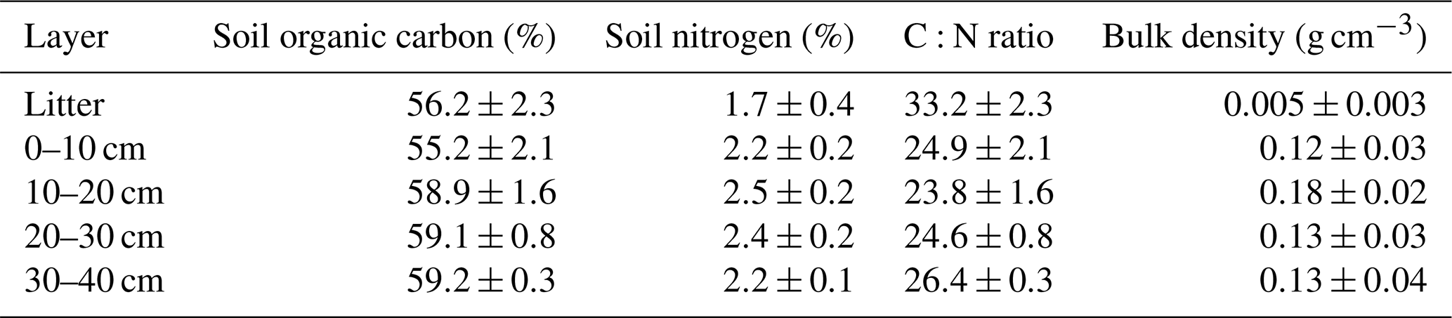
Before clear-cutting, the average soil organic carbon content at the site was 58 % and carbon distribution was rather uniform across different soil layers (Table 1). The total soil nitrogen content was lowest in the litter layer (1.7 %) and varied from 2.2 % up to 2.5 % among the other soil layers. The C:N ratio averaged at 27, which is typical for peatland forests with a fen history. The mean soil bulk density of the 0–40 cm layer was 0.14 g cm⁻³. The present-day peat thickness at Lettosuo varies mostly between 1.5 and 2.5 m. Assuming a thickness of 2 m results in soil organic carbon and nitrogen stock estimates of 156±72 kg C m⁻² and 6.4±2.9 kg N m⁻² (± SD), respectively.

Table 1Mean soil organic carbon, nitrogen, C:N ratio, bulk density and their standard deviation in different soil layers determined before the harvest (n = 3–33).

Download Print Version | Download XLSX

Clear-cutting was performed within a trapezoidal area of 23 500 m² (Fig. 1) between 29 February and 16 March 2016. After clear-cutting, the logging residues were left at the site. The previous ground vegetation was almost totally destroyed in the harvesting operation and the following drastic increase in solar radiation. In the following summer, some species adapted to the open, well-lit conditions; for example, Rubus idaeus, Carex canescens and Dryopteris carthusiana were observed here and there within the clear-cut site. Mounding was performed on 1–2 August 2016, and spruce (Picea abies) seedlings were planted in 2017. In addition to the clear-cut site, we conducted GHG measurements on a similarly sized control site located southwest of the clear-cut site, where the forest was left in its original state with similar tree stand and vegetation composition to at the preharvest clear-cut site.

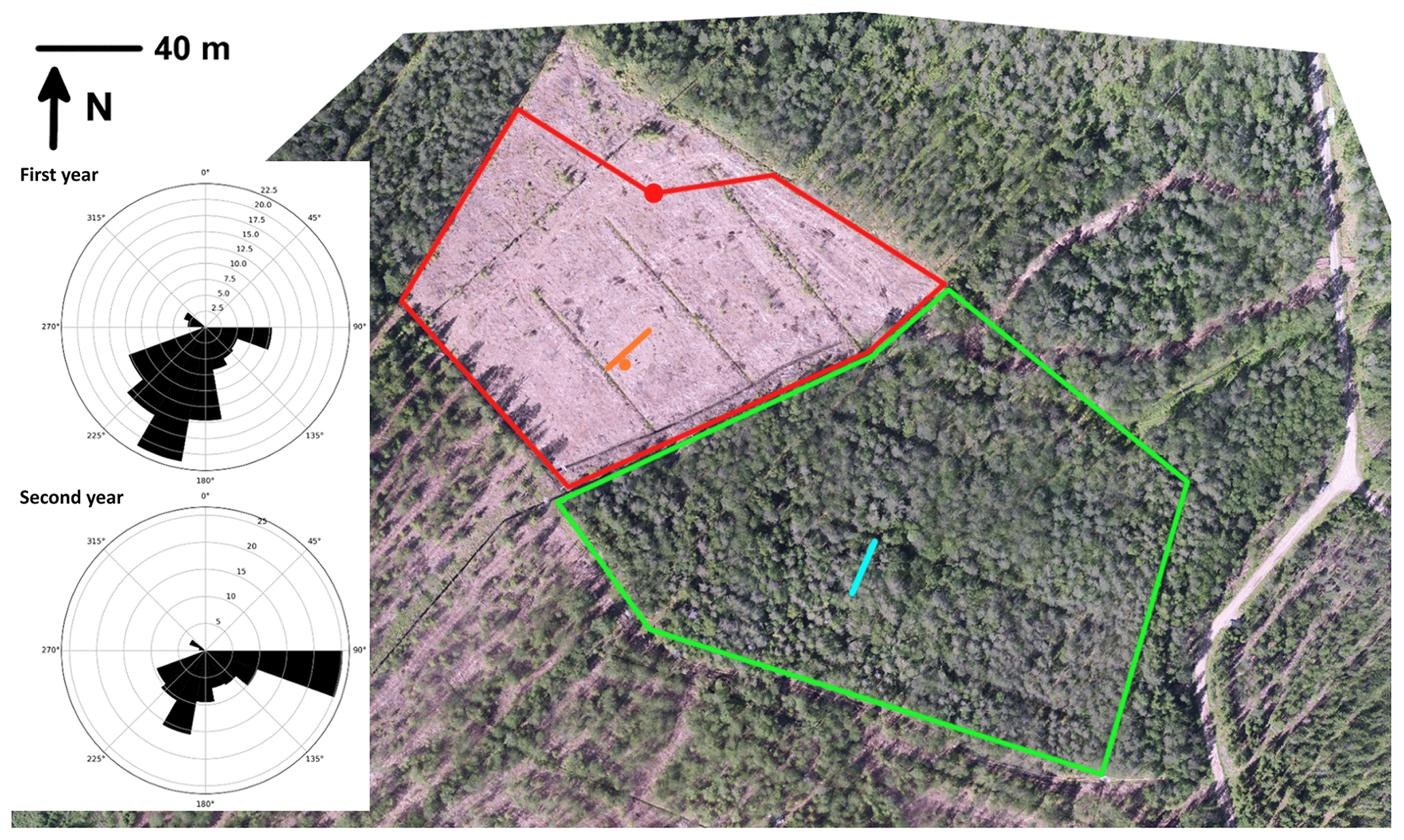
Figure 1Aerial view of the clear-cut site and the surrounding forest at Lettosuo. The red dot shows the location of the eddy covariance mast, and the red lines surround the target area (80–315^∘). The meteorological measurements were conducted at the location indicated by the orange dot, while the orange line marks the water table, soil temperature and chamber measurements (4, 8, 12 and 22.5 m from the ditch). Similar measurements of greenhouse gas fluxes, water table and soil temperature within the control site, surrounded by the green lines, are shown with a light blue line. The wind roses on the left show the cumulative footprint contributions (in percentage) of the accepted flux data.

2.2 Measurement system

An EC system to measure turbulent CO₂ and energy fluxes was set up in the northeastern part of the clear-cut (Fig. 1), and the measurements started on 8 April 2016, approximately 3 weeks after the clear-cutting had ended. The measurements continued until 7 April 2018. From this point on, the time periods of 8 April 2016–7 April 2017 and 8 April 2017–7 April 2018 are referred to as the first and second EC measurement year, respectively. The EC system included a three-axis sonic anemometer (uSonic-3 Scientific, METEK, Elmshorn, Germany) for wind speed and air temperature and a closed-path infrared gas analyser (LI-7000, Licor Biosciences, Lincoln, NE, USA) for CO₂ and H₂O mixing ratios. A sampling rate of 10 Hz was used for the EC system. The measurement height was 2.75 m, the flow rate was about 6 L min⁻¹ and the length of the inlet tube (inner diameter 3.1 mm, Bevaline IV) was 8 m. The mouth of the inlet tube was positioned 15 cm below the sonic anemometer. Air with a zero CO₂ concentration was used as the reference gas when calibrating the gas analyser. The micrometeorological sign convention is used throughout the paper: a positive flux indicates a flux from the ecosystem to the atmosphere (net emission) and a negative flux indicates a flux from the atmosphere into the ecosystem (net uptake).

Auxiliary meteorological measurements were installed at the centre of the clear-cut (80 m south of the EC mast) on 24 July 2015, i.e. before the clear-cutting. A similar system was installed 2 weeks earlier for the control site (180 m southeast of the EC mast). Air temperature and relative humidity were measured at 2 m height (HMP155, Vaisala Corporation, Vantaa, Finland) and soil temperature profile was measured at 5, 10, 20 and 30 cm depths (Pt100, Vaisala Corporation, Vantaa, Finland); the measurements also included net radiation (NR Lite2 Net Radiometer, Kipp & Zonen, Delft, The Netherlands), photosynthetically active photon flux density (PPFD) (PQS1 PAR Quantum Sensor, Kipp & Zonen, Delft, the Netherlands) and ground heat flux (HFP01, Hukseflux Thermal Sensors B.V., Delft, the Netherlands). In addition to these, global radiation (Pyranometer CMP3, Kipp & Zonen, Delft, The Netherlands) was measured from another EC mast above the canopy of the surrounding forest (250 m south from the clear-cut EC mast). The data were collected by data loggers (QML201C, Vaisala Corporation, Vantaa, Finland) as 30 min averages.

2.3 EC data processing

Half-hourly turbulent fluxes were calculated using standard EC methods (Aubinet et al., 2012). The 10 Hz raw data were block-averaged, and a double rotation of the coordinate system was applied (McMillen, 1988). The time lag between the gas analyser and sonic anemometer signals was determined by cross-correlation analysis for each flux variable and 30 min period. Water vapour fluctuations affecting flux measurements with LI-7000 were compensated for (Webb et al., 1980); a corresponding compensation is not necessary for temperature (Rannik et al., 1997). The fluxes were corrected for systematic losses due to block averaging and attenuation of the highest frequencies in the cospectra between vertical wind speed and mixing ratio; the transfer function method of Moore (1986) was used for this. For the high-frequency losses, the transfer functions describing the flux attenuation were determined separately for CO₂ and water vapour fluxes (with half-power frequencies of 1.3 and 0.6 Hz, respectively) using temperature cospectra as the reference. These functions were convoluted with generic cospectral distributions (Kaimal and Finnigan, 1994) to calculate the flux correction as a function of wind speed and atmospheric stability.

The 30 min averaged data were screened according to the following acceptance criteria: relative stationarity (Foken and Wichura, 1996) <100 %, internal LI-7000 pressure >60 kPa, CO₂ mixing ratio >350 ppm, wind direction within 80–315^∘, number of spikes in the vertical wind speed and CO₂ concentration data <150 of 18 000. Also, the periods of weak turbulence were discarded by applying a friction velocity (u_∗) limit of 0.125 m s⁻¹ (Fig. S1 in the Supplement). In addition, the footprint accumulated within the target area shown in Fig. 1 was required to exceed a limit of 0.75 to ensure that the measured flux originated predominantly from the clear-cut site. The footprints were calculated using the model developed by Kormann and Meixner (2001) and input data measured with the sonic anemometer.

In addition to the vertical turbulent fluxes, the CO₂ fluxes associated with the storage of CO₂ below the measurement height were calculated from the change in the mean CO₂ concentration profile between consecutive half-hour periods. It was assumed that the CO₂ concentration in the air column from ground level to the measurement height of 2.75 m was constant.

There were only two periods when a measurement gap in the data was longer than 5 d: 30 September–5 October 2016 and 28 April–4 May 2017. After applying all the data filters described above, 30 % of the 32 635 half-hour periods recorded within the measurement period were accepted for further analysis (Table S1, Fig. S2 in the Supplement). The gap-filling procedure and uncertainty analysis of the net ecosystem exchange of CO₂ (NEE) are described in Appendices A and B.

2.4 Surface energy balance and Bowen ratio

The surface energy balance can be expressed as

where Q_H is sensible heat flux, Q_E is latent heat flux, Q_N is net radiation, Q_G is the ground heat flux, and Q_S is the sum of storage fluxes from other energy sinks and sources. In this study, we assumed that Q_S=0.

The Bowen ratio, defined as

is used to describe the partitioning of Q_N−Q_G to Q_H and Q_E at the surface. When β<1, more available energy at the surface is released to the atmosphere as latent heat than as sensible heat (and vice versa when β>1). In this study, we present monthly Bowen ratios that were calculated from the monthly mean daytime (10:00–16:00, UTC+2) fluxes of Q_H and Q_E.

Gap-filling of the energy fluxes is described in Appendix C.

2.5 Chamber measurements of GHG fluxes

For manual chamber measurements, sampling transects were set up within the clear-cut and control sites, where the GHG fluxes were measured between 29 June 2015 and 29 August 2017, mostly during the snow-free periods. The measurement interval varied between 1 week and 1 month, but there were longer gaps in autumn 2015 and spring 2016. The transect had two flux measurement plots at a distance of 4, 8, 12 and 22.5 m from the ditch, and at each distance there was an automatic WTL logger close to the flux measurement plots (see Sect. 2.7 for details). In addition, all the flux plots included a soil temperature data logger (iButton DS1921G, Maxim Integrated Products) at 5 cm depth and two of them (8 and 22.5 m from the ditch) also had a similar logger at 30 cm depth. Before starting the measurements, 2 cm deep grooves were carved into the soil surface for the chambers, and the grooves were occasionally renewed when necessary to keep the chamber-sealing adequate. It should be noted that, even though logging residues were left at the site, the measurement plots did not have any above-ground residues. The fluxes were measured using a closed-chamber system with an opaque cylindrical chamber (height 30.5 cm, diameter 31.5 cm) including a mixing fan. The measurements were made in two different ways: using (1) a portable analyser and (2) a stationary analyser. As a portable analyser, we employed a Gasmet DX4015 (Gasmet Technologies Oy, Helsinki, Finland), based on Fourier transform infrared spectroscopy, to measure CO₂, CH₄ and N₂O mixing ratios every 5 s. At the clear-cut site, only the portable gas analyser was used. In this setup, the sampled air was circulated in a loop between the gas analyser and the chamber, and the closure time was 10–11 min. At the control site, the portable analyser was used in 2015 for all the gases, but from 2016 onwards the analyser was used only for measuring the N₂O mixing ratios. Starting from 2016 at the control site, we connected the portable gas analyser in series with a Picarro G1130 cavity ring-down spectroscopy gas analyser (Picarro Inc., Santa Clara, CA, USA) to acquire more precise CO₂ and CH₄ mixing ratios. In this system, the gas analysers were stored in a cabin and connected to the chamber with 50 m long tubing. The instruments were compared against each other and observed to result in very similar flux estimates with the 10–11 min closure time. The error caused by not returning the sampled air back to the chamber was corrected for in the data analysis.

The fluxes were calculated the same way for all the gases (Korkiakoski et al., 2017). In short, both linear and exponential regression models were first fitted to the mixing ratio time series using the least-squares approach. The start and end points of the chamber closure were visually identified from the data for each closure. The first minute of each measurement was discarded to ensure that the sample air was properly mixed inside the chamber. After fitting, the mass flux (F) was calculated as

where ${\left(\frac{\mathrm{d}C\left(t\right)}{\mathrm{d}t}\right)}_{t=\mathrm{0}}$ is the mixing ratio change in time determined from a linear or exponential model at the beginning of the closure; M is the molecular mass of CO₂, CH₄, or N₂O (44.01, 16.04 and 44.01 g mol⁻¹, respectively); P is air pressure; R is the universal gas constant (8.314 J mol⁻¹ K⁻¹); T is the mean chamber headspace temperature during closure; and V and A are the volume and the base area of the chamber headspace, respectively. The snow depth and the height of mosses and other vegetation in the chamber headspace volume were taken into account, ignoring the pore space in the soil and snow. However, if the soil surface was frozen, the measurements were not made as it was not possible to properly seal the chamber. Finally, analyser-specific flux limits were determined to choose between the linear and exponential models (Korkiakoski et al., 2017). If the flux calculated with the linear model was smaller than the limit, then this estimate was considered more robust for the noisy data and adopted for the later analysis. These limits for the portable system were 5.6 µg CO₂ m⁻² s⁻¹, 9.7 ng CH₄ m⁻² s⁻¹ and 12.5 ng N₂O m⁻² s⁻¹. We did not define a corresponding limit for the CO₂ flux measured with the Picarro gas analyser at the control site as the fluxes were always sufficiently large for using exponential fitting, but for CH₄ the limit was set to 0.7 ng CH₄ m⁻² s⁻¹.

The CO₂ flux measured with chambers represents forest floor respiration (R_ff), which is defined as the sum of heterotrophic and autotrophic respiration. As clear-cutting affects soil processes, it should be noted that the R_ff before and after clear-cutting consists of different components. Before the clear-cutting (the 2015 data), R_ff includes ground vegetation and living roots of trees and ground vegetation, but after clear-cutting (2016–2017) it instead includes the survived and regrown ground vegetation and living and dead roots.

The summertime sum of R_ff was calculated for each summer separately by using Eq. (A3) with hourly soil temperature at 5 cm depth. The uncertainty of this sum was estimated from the minimum and maximum sums based on the standard errors of model parameters (R₀ and E). The minimum and maximum sums were slightly asymmetrical around the mean sum, so the largest deviation from the mean sum was adopted as a conservative uncertainty estimate.

2.6 Water table level measurements and analysis

The water table levels within both the clear-cut and non-managed control site were measured for 1 year before (2015) and 2 years after the clear-cutting (2016–2017). Four automatic monitoring plots consisting of dipwells (perforated plastic tubes 120 cm long and 3.5 cm in diameter) were set up at the centre of each site (Fig. 1), located at a distance of 4, 8, 12 and 22.5 m in a transect perpendicular to the ditch (ditch spacing was 45 m). In addition, in order to calibrate the automatic water table measurement data, manually monitored dipwells were installed close to the automatically monitored dipwells within the clear-cut and control sites. WTL was measured manually at weekly or fortnightly intervals during March–November. From the automated dipwells, WTL was recorded with automatic probes (TruTrack WT-HR-logger, Intech Instruments Ltd, Auckland, New Zealand; Odyssey Capacitance Water Level Logger, Dataflow Systems Limited, Christchurch, New Zealand) at hourly intervals. The recorded values were then calibrated with linear regression using the manually measured WTL data from both the control and clear-cut site.

2.7 Statistical analysis

The linear mixed-effect model was used for testing for differences in the daily mean CO₂, CH₄ and N₂O fluxes between the clear-cut and control sites and between the years in the chamber measurement data. In both cases, the chamber plots were treated as a random effect. The fixed effects of the model were the site type (clear-cut or control) and the measurement year when comparing the measurements made at different sites and in different years, respectively. The linear mixed-effect model was carried out with the R programming language (R Core Team, 2018, version 3.5.0) using the “lme4” package. The normality of model residuals was visually checked using quantile–quantile plots. The differences were tested with Tukey's honestly significant difference post hoc test.

The analysis of the clear-cutting effects on WTL was based on the paired treatment approach (also called calibration period – control area method) (e.g. Kaila et al., 2014; Laurén et al., 2009). We first calculated linear regressions between the WTL within the control and clear-cut sites for the pretreatment period using the WTL logger data from 2015. Then we used this regression model and the post-treatment WTL data from the control site to predict WTL for the clear-cut site as if it had not been harvested. The clear-cut effect was calculated as the difference between the calibrated post-clear-cut WTL measurements and the predicted background WTL values in the clear-cut site after the harvest.

3.1 Meteorological and hydrological conditions

The long-term (1981–2010) mean annual, winter (DJF) and summer (JJA) air temperatures at the nearby (Jokioinen, 35 km northwest of Lettosuo) weather station were 4.6, −5.3 and 15.2 ^∘C, respectively (Pirinen et al., 2012). The mean annual temperature before the clear-cutting in 2015 at Jokioinen was 6.2 ^∘C. Also, the winter (2015–2016) before the clear-cutting was warmer (−3.4 ^∘C), while summer 2015 was colder (14.4 ^∘C) than the long-term mean. The mean post-clear-cut annual air temperatures at the EC site during the first and second EC measurement year were 5.6 and 4.4 ^∘C, respectively (Fig. 2a); this difference was reflected in soil temperatures (Fig. 2b). Both post-clear-cut winters were warmer (2016–2017: −3.0 ^∘C; 2017–2018: −3.4 ^∘C) than the long-term average. However, the mean summer temperature at the EC site in 2016 was similar to (15.3 ^∘C), and in 2017 was cooler (by 1.6 ^∘C) than, in 1981–2010. In addition, compared to the precipitation at Jokioinen (long-term average 627 mm), the first EC measurement year was drier (502 mm) and the second year similar (656 mm) (Fig. 2c), while the pre-clear-cut year of 2015 was wetter (680 mm) than both post-clear-cut years. The autumn (SON) 2016 and winter 2016–2017 were especially dry, while the springs and summers were quite similar to the long-term average conditions.

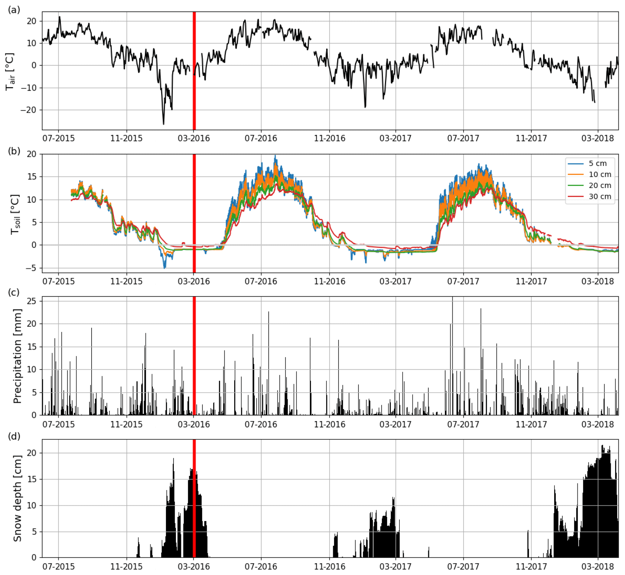
Figure 2Time series of (a) daily mean air temperature (T_air) and (b) hourly mean soil temperatures at 5, 10, 20, and 30 cm depths (T_soil) measured at Lettosuo, and (c) daily precipitation sum and (d) daily mean snow level recorded at the Jokioinen observatory (35 km northwest of Lettosuo). The clear-cutting (red vertical line) was carried out in February–March 2016.

Download

Both winters had a shallower snow cover than the long-term average annual maximum (28 cm; Pirinen et al., 2012). The maximum snow depths at Jokioinen were 12 and 22 cm in 2016–2017 and 2017–2018, respectively. Due to the especially shallow snow cover in the first winter and the high temperatures in March, all the snow had melted by 23 March 2017 (Fig. 2d). However, in 2018, the snow cover was still intact when the measurement period ended on 7 April.

The preharvest soil temperatures at 30 cm depth were similar within the clear-cutting and control sites, but clear-cutting increased their temporal variation (Fig. S3). After clear-cutting in late spring, the daily mean 30 cm soil temperature rose faster and was higher throughout the summer within the clear-cut than at the control site. Also, the 30 cm temperature within the clear-cut started to decline earlier in autumn and was lower during winter within the clear-cut than the control site. The monthly mean diel variation in soil temperature at 5 cm depth ranged from 0.8 to 1.3 ^∘C in July–September 2015 before clear-cutting (Fig. S4). After clear-cutting, this variation increased to 2.3–2.9 and 2.1–3.7 ^∘C in 2016 and 2017, respectively. On average the diel variation was 1.8 ^∘C larger in July–September after the clear-cutting than before it (Figs. 2b and S4). Increases in the diel temperature range were also observed at the 10 cm (1.2 ^∘C) and 20 cm (0.33 ^∘C) depths but not at 30 cm.

The mean WTL in July–August 2015 was −33 cm within the clear-cut area, while at the control site it was −50 cm (Fig. 3). After clear-cutting, the WTL rose and remained continuously at a markedly higher level than the predicted background WTL and the measured WTL at the control site. At the clear-cut site, the WTL rose to −22 and −27 cm in July–August 2016 and 2017, respectively. On the other hand, the WTL at the control site sank to −55 cm during these months in both post-harvest years. The largest post-treatment rise occurred in July–October when the average WTL was −23 and −24 cm in the clear-cut and −46 and −49 cm in the background model, corresponding to a 23 and 25 cm rise in WTL in 2016 and 2017, respectively (Fig. 3). As a consequence of heavy rain episodes in summer and autumn in 2017, the amplitude of WTL variations was larger then than the previous year.

Figure 3Mean daily water table level at the control site (measured; green) and the clear-cut site with (measured; black line) and without (estimated; grey line) the harvesting effect averaged over all the measurement points (4, 8, 12 and 22.5 m from the ditch) from June 2015 to October 2017. The clear-cutting (red vertical line) was carried out in February–March 2016.

Download

3.2 CO₂ exchange on an ecosystem level

3.2.1 Seasonal and diel variations

When the measurements started at the beginning of April 2016, the daily mean NEE was mainly <0.08 mg CO₂ m⁻² s⁻¹ but started to increase with temperature at the end of April, after the daily mean temperature exceeded 5 ^∘C (Figs. 2a and 4). There was a substantial temporary drop in NEE in the first half of June after a cold spell when the daily mean temperature decreased from 20 to 10 ^∘C. By the end of June, NEE stabilized at around 0.21 mg CO₂ m⁻² s⁻¹. From the end of August, NEE decreased until reaching a stable level of 0.03 mg CO₂ m⁻² s⁻¹ in January 2017. At the end of March 2017, NEE started to gradually increase, and in mid-May it quickly rose to 0.08 mg CO₂ m⁻² s⁻¹. After this, NEE continued to increase, stabilizing at around 0.13 mg CO₂ m⁻² s⁻¹ in August and then decreasing from the end of September onwards.

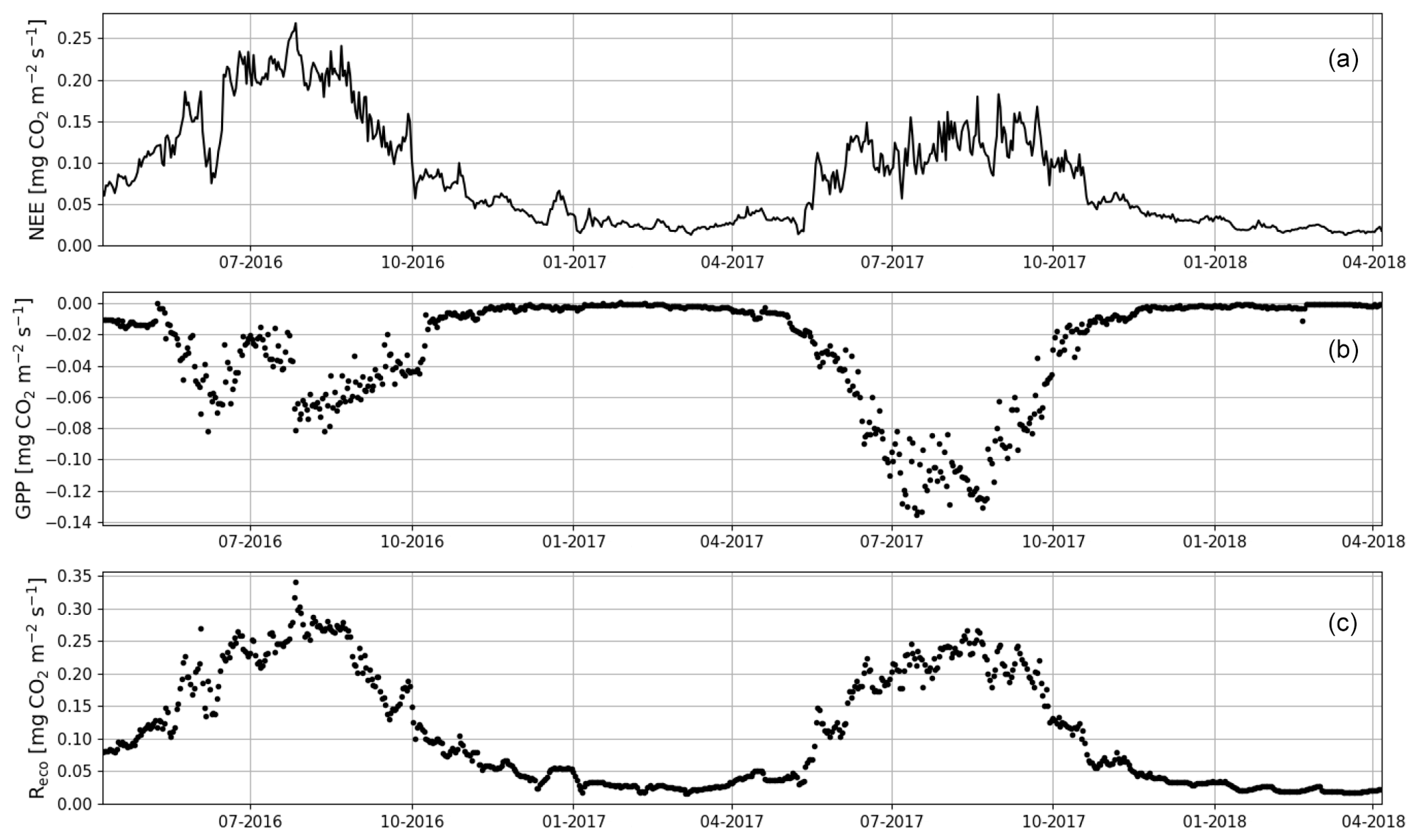
Figure 4The gap-filled time series of daily mean net ecosystem exchange (NEE, a) and the corresponding modelled gross primary production (GPP, b) and ecosystem respiration (R_eco, c) based on Eqs. (A2) and (A3), respectively.

Download

Even though all the big trees were removed in clear-cutting and most of the ground vegetation was destroyed, some small understorey trees were left at the site and weak photosynthesis could be observed simultaneously with the increased respiration in the end of April 2016 (Fig. 4). In May, the estimated magnitude of gross primary production ($\left|\mathrm{GPP}\right|$, Appendix A) increased to 0.05 mg CO₂ m⁻² s⁻¹, which was about 25 % of the respiration rate at that time. However, $\left|\mathrm{GPP}\right|$ decreased to 0.02 mg CO₂ m⁻² s⁻¹ in June, after which it started to increase again, reaching its maximum at 0.08 g CO₂ m⁻² s⁻¹ at the end of July and the beginning of August. From that point on, photosynthesis started to weaken, marking the ending of the growing season, and ceased in mid-October, about a month before the first snow. In 2017, $\left|\mathrm{GPP}\right|$ increased from mid-May until July, when it stabilized at around 0.11 mg CO₂ m⁻² s⁻¹. Similarly to in 2016, $\left|\mathrm{GPP}\right|$ decreased from August onwards.

The correlation between the night-time NEE (i.e. R_eco in Eq. A3) and the 5 cm soil temperature was stronger in summer 2017 than 2016 (Fig. 5a). The model fits (Eq. A3) indicate that the temperature response of ecosystem respiration (parameter E) was also stronger in 2017. However, the base respiration rate R₀ (R_eco at 10 ^∘C) was larger in the first than the second summer (0.199 vs. 0.173 mg CO₂ m⁻² s⁻¹). In addition, no correlation was found between the model residuals and WTL in either summer (Fig. S5). Like the temperature response of R_eco, the light response of GPP was stronger in summer 2017 than 2016 (Fig. 5b). Also, the corresponding maximum gross photosynthesis rate (GP_max, Eq. A2) more than doubled (−0.226 vs. −0.100 mg CO₂ m⁻² s⁻¹).

Figure 5Temperature (a; Eq. A3) and light responses (b; Eq. A2) of 30 min CO₂ fluxes for the summers of (JJA) 2016 (black) and 2017 (blue). The temperature response equation was fitted to the night-time data (PPFD < 20 µmol m⁻² s⁻¹), and the light response equation was fitted to the daytime (PPFD > 20 µmol m⁻² s⁻¹) data.

Download

The site was on average a CO₂ source throughout the day during the summer as well. It should be noted, however, that there were still multiple half-hour periods, especially in August 2017, when the site acted as a CO₂ sink. A noticeable diel variation in NEE was observed mainly from April to October (Fig. 6). Between April and August, the mean diel NEE cycle had a minimum during the morning hours (05:00–10:00, UTC+2) and the highest emissions during the evening and night (21:00–01:00). After August, the lowest emissions took place later, at around noon. On the other hand, the highest emissions were observed earlier, at 20:00 in September and at 18:00 in October. In October, the diel cycle of NEE was still noticeable; it vanished in November and reappeared in March 2017. In spite of the different mean fluxes, the amplitudes of their diel cycle were rather similar in 2016 and 2017, except from July to September when the amplitudes were much larger in 2017. Also, unlike in 2016, systematic diel variation was still obvious in November 2017. Even though such variation indicates significant photosynthesis during the midday hours, the monthly mean diel NEE cycle consistently showed positive fluxes.

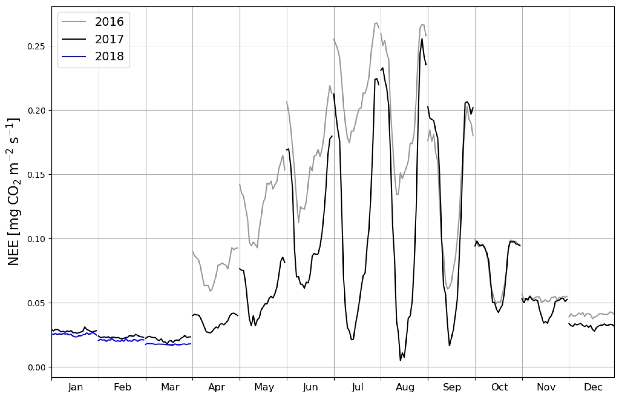
Figure 6Monthly mean diel cycles of gap-filled net ecosystem exchange (NEE) measurements in the first (2016, grey), second (2017, black) and third (2018, blue) calendar year after the clear-cutting.

Download

3.2.2 CO₂ balances

The annual CO₂ balances of the first and the second year after clear-cutting were 3086±148 g CO₂ m⁻² (± uncertainty; see Appendix) and 2072±124 g CO₂ m⁻², respectively. About half of the annual CO₂ emissions during both EC measurement years took place during the summer months (JJA), totalling 1558±99 g CO₂ m⁻² (Table 2, Fig. 7), and 73 % (2256±146 g CO₂ m⁻²) of the annual total was accumulated during the May–September period. In 2017, however, these emissions decreased to 915±79 g CO₂ m⁻² (June–August) and 1401±109 g CO₂ m⁻² (May–September), i.e. by 41 % and 38 %, respectively. The effect of storage fluxes on the CO₂ balance was negligible as the daily mean storage flux typically varied within ±0.009 mg CO₂ m⁻² s⁻¹ during summer and within ±0.004 mg CO₂ m⁻² s⁻¹ during the other seasons.

Table 2Annual and summertime (JJA) balances of net ecosystem exchange (NEE), modelled gross primary production (GPP), and modelled total ecosystem respiration (R_eco), as well as the modelled summertime sums of forest floor respiration (R_ff).

Download Print Version | Download XLSX

Figure 7The monthly sums of net ecosystem exchange (NEE), gross primary production (GPP) and ecosystem respiration (R_eco) based on EC data in April 2016–March 2018.

Download

The most significant period of CO₂ uptake was from June to September (Fig. 7). Considering only the summer months (JJA), the integrated GPP was 389 and 761 g CO₂ m⁻² in 2016 and 2017, respectively (Table 2); i.e. the mean CO₂ uptake in the second summer after clear-cutting increased by 96 % from the first summer. On the other hand, the total summertime R_eco decreased by 14 %, from 1928 g CO₂ m⁻² in 2016 to 1652 g CO₂ m⁻² in 2017 (Table 2).

3.3 Soil GHG fluxes

The summertime (JJA) R_ff measured at the soon-to-be clear-cut site in 2015 was 1611±191 g CO₂ m⁻² (± uncertainty; see Sect. 2.5), and the measured CO₂ fluxes varied from 0.04 to 0.36 g CO₂ m⁻² s⁻¹ (Fig. 8a). The CH₄ flux averaged over all the measurement plots was $-\mathrm{26}\pm \mathrm{5}$ ng CH₄ m⁻² s⁻¹ before the clear-cutting. All the measured CH₄ fluxes were negative (Fig. 8b) ranging from −103 to −2 ng CH₄ m⁻² s⁻¹. N₂O fluxes varied mostly from −17 to 33 ng N₂O m⁻² s⁻¹ and averaged at 1±5 ng N₂O m⁻² s⁻¹ (Fig. 8c). At the control site, the summertime fluxes of CO₂ (from 0.03 to 0.39 g CO₂ m⁻² s⁻¹) and N₂O (mean: 11±9 ng N₂O m⁻² s⁻¹) in 2015 were not significantly different from those at the soon-to-be clear-cut site. However, the CH₄ fluxes (mean: $-\mathrm{10}\pm \mathrm{3}$ ng CH₄ m⁻² s⁻¹) at the control site were significantly (p<0.02) larger than at the soon-to-be clear-cut site.

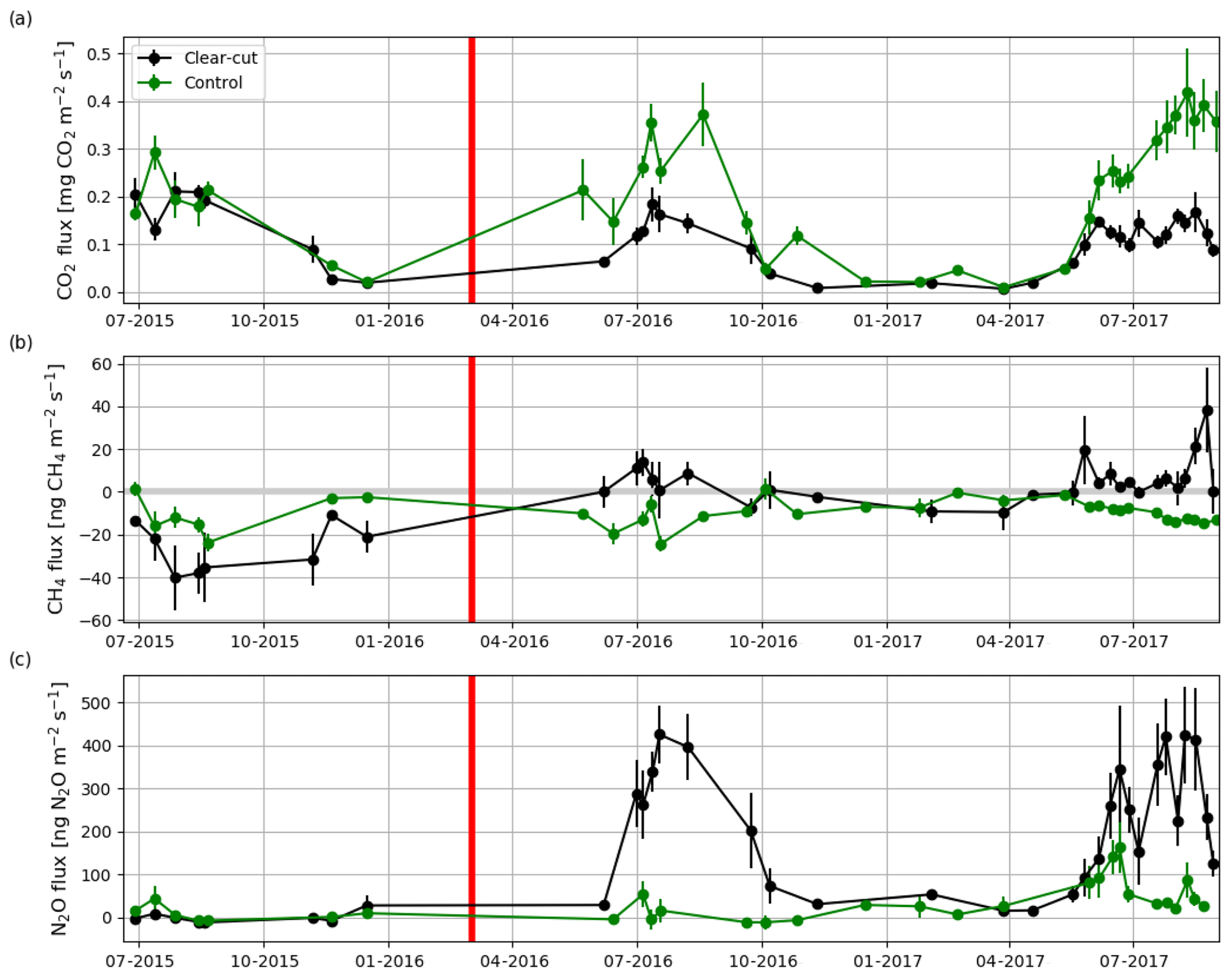
Figure 8Hourly mean fluxes measured with manual chambers of (a) CO₂, (b) CH₄ and (c) N₂O averaged over all measurement points (4, 8, 12 and 22.5 m from the ditch) at the clear-cut (black) and control (green) sites from June 2015 to August 2017. The error bars show the standard error of the mean. The clear-cutting (red vertical line) was carried out in February–March 2016.

Download

After the clear-cutting, the total summertime R_ff decreased to 980±299 g CO₂ m⁻² in summer 2016 and remained at the same level (1047±113 g CO₂ m⁻²) in 2017. These numbers were 51 % and 63 % of the R_eco for the summers of 2016 and 2017, respectively (Fig. 9). Also, the temperature response of R_ff got weaker, and the R₀ parameter (R_ff at 10 ^∘C) decreased, while at the control site the responses remained quite similar over the years (Fig. 10). The strength of temperature response and R₀ partly recovered in 2017 but were still weaker than before the clear-cutting. In contrast to the R_ff at the clear-cut, the summertime R_ff at the control site increased from 1852±1353 g CO₂ m⁻² in 2015 to 2280±346 g CO₂ m⁻² and 2438±225 g CO₂ m⁻² in 2016 and 2017, respectively. However, the increase was significant only when comparing the summers of 2015 and 2017 (p<0.05). The clear-cut and control sites were significantly different from each other in both summers (p<0.001) after clear-cutting.

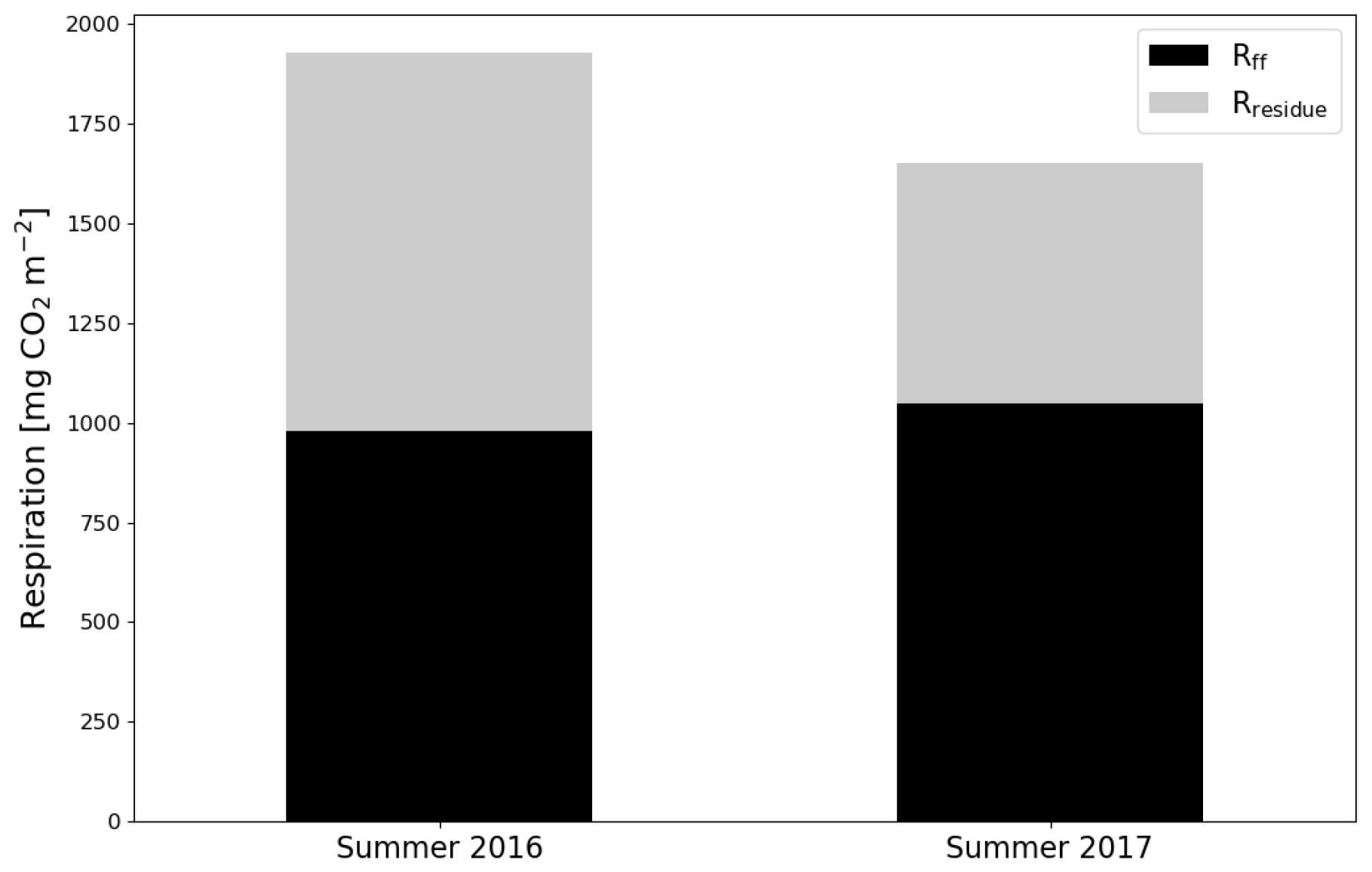
Figure 9The division of ecosystem respiration (R_eco, based on EC measurements) to forest floor respiration R_ff (chamber measurements) and respiration of logging residues ($R_{\mathrm{residue}}=R_{\mathrm{eco}}-R_{\mathrm{ff}}$) for the summers of 2016 and 2017.

Download

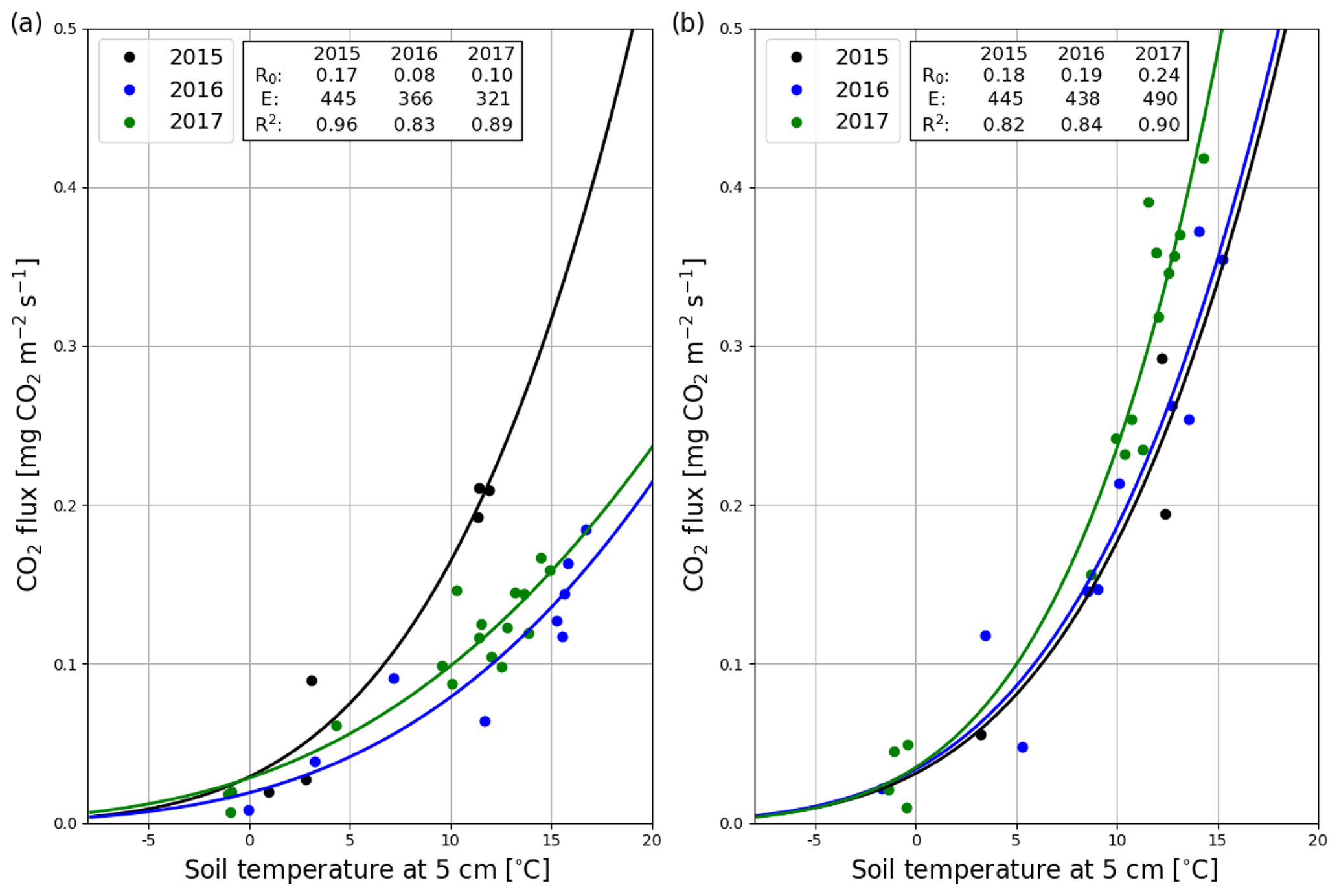
Figure 10Temperature response (Eq. A3) of the hourly mean CO₂ fluxes measured with manual chambers at the clear-cut (a) and control (b) site in 2015 (black), 2016 (blue) and 2017 (green).

Download

CH₄ fluxes changed markedly after the clear-cutting, as the previously small mean CH₄ sink turned into a small CH₄ source in the first (4±3 ng CH₄ m⁻² s⁻¹) and second (6±2 ng CH₄ m⁻² s⁻¹) year after the clear-cutting (Fig. 8b); the changes were significant for both years (p<0.001). However, the post-clear-cut years were not significantly different from each other (p=0.85). The post-clear-cut fluxes varied mostly from −14 to 28 ng CH₄ m⁻² s⁻¹, with some occasional emission peaks reaching up to 140 ng CH₄ m⁻² s⁻¹. Most of the measured fluxes were positive (emission), even though a single measurement plot could act both as a source and a sink on different measurement days. The control site remained as a CH₄ sink in 2016 and 2017 and neither of the mean summer fluxes were significantly different from the preharvest summer mean. However, the mean CH₄ fluxes were significantly different (p<0.001) between the sites in both post-harvest summers.

Similarly to CH₄, the post-clear-cut N₂O fluxes were significantly higher than the pre-clear-cut ones (p<0.001), and the post-clear-cut years did not differ significantly from each other. After the clear-cutting, the mean annual fluxes were 228±26 and 212±21 ng N₂O m⁻² s⁻¹ in 2016 and 2017, respectively (Fig. 8c). All the measurement plots turned to large N₂O sources, and the largest measured emission was 1339 ng N₂O m⁻² s⁻¹. All the measured fluxes were positive, except for a plot furthest from the ditch that acted as a temporary N₂O sink in 2017, especially in the June–July period. The N₂O fluxes at the control site remained low in summer 2016 (mean: 16±11 ng N₂O m⁻² s⁻¹) but increased in summer 2017 (mean: 70±10 ng N₂O m⁻² s⁻¹). However, the post-harvest emissions at the control site were significantly lower than those at the clear-cut site (p<0.001). Both the spatial and temporal variations were large: the largest emissions occurred in June while from July onwards the emissions decreased (Fig. 8c).

3.4 Energy fluxes

The daily sums of sensible heat (Q_H) were about 1 MJ m⁻² d⁻¹ on average at the start of the EC measurement period in April 2016 and increased to a maximum of 4.7 MJ m⁻² d⁻¹ in June (Fig. 11). In July, the daily Q_H sum was already decreasing with the decreasing net radiation (Q_N) and turned negative in October. On the other hand, the daily sums of latent heat flux (Q_E) were quite stable from April until August, averaging at 1.0±0.04 MJ m⁻² d⁻¹ (± standard error of mean). In September, Q_E started to decrease and reached zero at the end of October. The ground heat flux (Q_G) varied within 0–0.5 MJ m⁻² d⁻¹ from April to August, after which it varied mostly between −0.5 and 0 MJ m⁻² d⁻¹ until the end of April 2017.

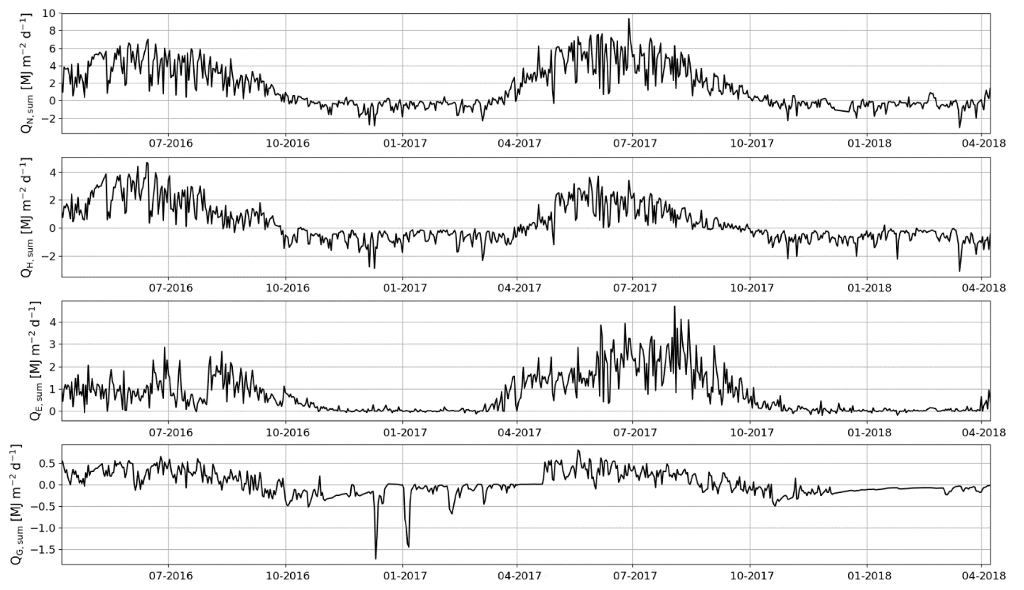
Figure 11Daily sums of net radiation (Q_N), sensible heat flux (Q_H), latent heat flux (Q_E) and ground heat flux (Q_G).

Download

In 2017, the seasonal dynamics of the energy fluxes were similar to 2016, but the magnitude of fluxes changed considerably. The summertime average daily sum of Q_H decreased from 1.8 to 1.2 MJ m⁻² d⁻¹, while that of Q_E increased from 1.3 to 2.3 MJ m⁻² d⁻¹. Also, the monthly sums of these fluxes were markedly different in the second year after the clear-cutting. During the period of the highest fluxes (April–September), the Q_H sum was 33 % smaller in 2017 than 2016, while the Q_E and Q_N sums were higher by 40 % and 13 %, respectively. The changes in Q_G were minor.

The monthly mean midday Q_H in May and June 2016 were 206 and 165 W m⁻², respectively (Fig. 12a). After June, the midday Q_H started to decrease with decreasing Q_N, and the night-time Q_H turned from zero to slightly negative. The midday Q_E also increased from April to June, reaching 88 W m⁻², and remained quite stable until September. The resulting monthly mean daytime Bowen ratio (β), increased from 1.7 in April to 2.6 in May 2016 and then declined to 0.8 in August. In 2017, the mean midday Q_H was similar to that in 2016, except in July and September when the fluxes were 34 % and 23 % lower, respectively, than in 2016 (Fig. 12b). However, the daily maximum Q_E was either similar to or higher (up to 48 %) than Q_H in all months except May 2017. Correspondingly, β was lower than 1 (0.6–1.0) during the period of high fluxes in 2017, except in May when it was 1.7.

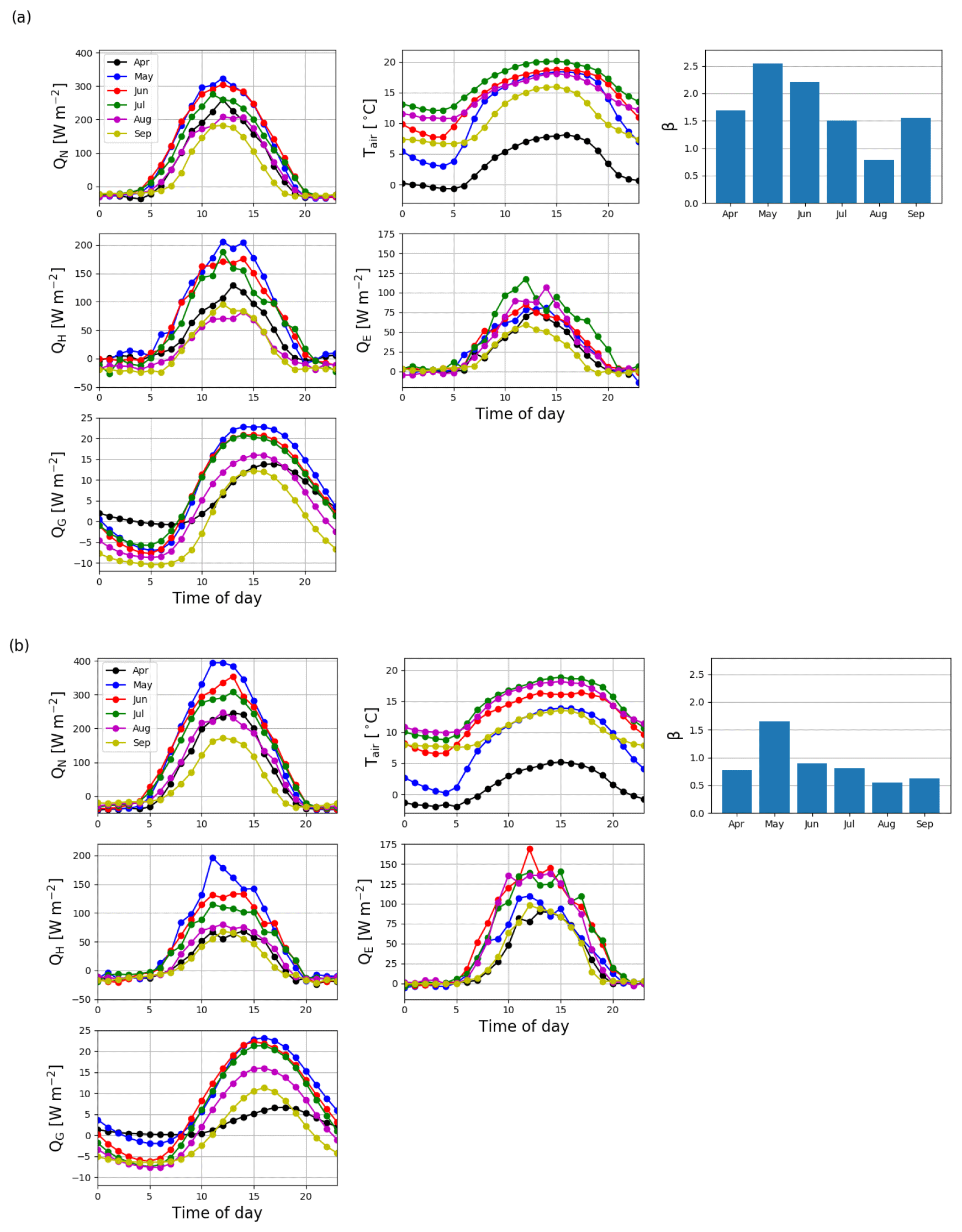
Figure 12Monthly mean diel cycles of net radiation (Q_N), air temperature (T_air), sensible heat flux (Q_H), latent heat flux (Q_E), ground heat flux (Q_G) and the monthly mean daytime (10:00–16:00, UTC+2) Bowen ratios (β) from April to September in 2016 (a) and 2017 (b).

Download

4.1 Dynamics of the CO₂ fluxes and flux components

The study site was a large source of CO₂ during the 2 EC measurement years after clear-cutting, but the emissions were 33 % smaller in the second than the first year. $\left|\mathrm{GPP}\right|$ remained low and stable during the first summer after clear-cutting, reflecting the fact that neither vascular ground vegetation nor moss cover had developed substantially by that time. However, during the second summer, the total $\left|\mathrm{GPP}\right|$ increased by 96 % from the first post-clear-cut summer, and the increase in the coverage of ground vegetation was already noticeable (although not directly measured). This relatively fast recovery of ground vegetation is similar to the leaf area index changes observed by Mäkiranta et al. (2010) after clear-cutting in a nutrient-poor peatland forest. R_eco was larger in the first summer than in the second post-harvest year, which could be due to the first year being warmer or due to changes in the respiration of either residues or forest floor in the second year. The chamber measurements, which were not affected by aboveground logging residues, showed a 39 % and 35 % decrease in R_ff after clear-cutting in the first and second summer after clear-cutting, respectively. Possible reasons for this decrease include reduced peat decomposition due to raised WTL, ceased autotrophic respiration of (the harvested) trees roots and decreased autotrophic respiration of ground vegetation, even though the latter slightly recovered during the summer as the ground vegetation started to regrow. The CO₂ flux from the decomposing below-ground logging residues (roots) was not sufficiently large to compensate for this decrease in R_ff. In summer 2016, R_ff was 51 % of the R_eco, suggesting that half of the R_eco during that time originated from the above-ground logging residues, which were not included in the chamber measurements of R_ff. In summer 2017, however, R_eco decreased by 14 %, but R_ff remained about the same, indicating that a larger proportion (63 %) of R_eco originated from the forest floor respiration than in the previous summer. This could be due to the decrease in decomposition rate of the aboveground logging residues due to lower temperatures and because the residues had already partly decomposed during the previous summer. However, the lower temperatures would also decrease R_ff, but this did not happen because in 2017 WTL was 5 cm lower, which enhanced peat decomposition. In addition, the NEE in summer 2017 was approximately equal to R_ff, which means that the increase in $\left|\mathrm{GPP}\right|$ was sufficient to balance the CO₂ emissions from the logging residues but not from soil and plants.

After the removal of the canopy, more solar radiation reached the ground surface, heating it more during the daytime, while the heat transfer from the soil to the atmosphere was enhanced during the night; together these resulted in a higher diel variation in soil temperature. On the other hand, the insulating impact of logging residues may have partly dampened the amplitude of the diel temperature cycle, as observed by Ojanen et al. (2017). The higher soil temperatures during the daytime may have enhanced peat respiration in the layer closest to the surface. However, it has been shown in previous studies that the temperature response of respiration weakens when the soil gets dry, often resulting in lower respiration rates (Mäkiranta et al., 2009, 2010). Such weakening of the temperature response was also observed at Lettosuo, especially in the first summer after the harvest when the almost bare soil surface was exposed to more solar radiation after clear-cutting. Also, summer 2016 was warmer and drier than on average, which probably enhanced this effect. Moreover, the addition of logging residues may have increased R_eco substantially, as demonstrated by Mäkiranta et al. (2012), who observed that the plots with logging residues had a CO₂ efflux twice as high as the plots without them. However, a later study by Ojanen et al. (2017) did not show a consistent increase in soil organic matter decomposition rates at similar sites. In previous studies, a decrease has been observed in both R_eco (Kowalski et al., 2004, 2003; Takagi et al., 2009) and R_ff (Mäkiranta et al., 2010; Takagi et al., 2009; Zerva and Mencuccini, 2005) after clear-cutting in peatland and upland forests. However, also increasing R_eco and R_ff have also been reported (Kowalski et al., 2004; Londo et al., 1999). The differences between these results are most likely caused by a different effect of the harvest on soil microbial activity, which is mostly controlled by soil temperature, moisture and nutrient availability (Davidson et al., 1998; Fontaine et al., 2004, 2007; Lloyd and Taylor, 1994). Other possible reasons for this variability include differences in, for example, root respiration, the type and amount of logging residue, and WTL, especially in peatland forests.

In peat soils, the decomposition of organic matter is mainly controlled by soil temperature and WTL (Blodau et al., 2004; Mäkiranta et al., 2009; Silvola et al., 1996), but soil temperature is typically the most influential factor for explaining the temporal dynamics in R_ff (e.g. Mäkiranta et al., 2008; Ojanen et al., 2010). At Lettosuo, the correlation between the half-hourly R_eco and soil temperature was mostly weak. This could be due to logging residues, as their decomposition rate probably does not depend as much on soil temperature as on the temperature and moisture of the logging residues themselves. At times, especially when the temperature range was larger (in May and June), a significant relationship (correlation coefficient peaking at 0.57) was observed, and there was also an obvious temperature response that followed the annual cycle. Also, when WTL is closer ($>-\mathrm{15}$ cm) to the surface, it is usually a significant predictor of R_ff in peat soils (Chimner and Cooper, 2003; Riutta et al., 2007). At Lettosuo after clear-cutting, WTL varied mostly within 20–30 cm below the soil surface, and there was no correlation between R_eco and WTL after removing the effect of soil temperature on R_eco (Fig. S5). Because R_eco combines many respiration components in addition to R_ff, it is likely that the high CO₂ efflux from logging residues, for example, masks the possible WTL effect on R_ff.

Our results show that, after clear-cutting, a peatland forest is a large source of CO₂ to the atmosphere. Nutrient-rich drained peatland forests with a growing tree stand have generally been found to be CO₂ neutral or small sinks of CO₂ (Meyer et al., 2013; Ojanen et al., 2013; Uri et al., 2017), as the carbon accumulated by trees typically balances the carbon emissions caused by the decomposing peat layer. This suggests that Lettosuo was probably also close to a CO₂-neutral state before the clear-cutting. Thus, the impact of clear-cutting from CO₂ neutral to a source of 3086±148 g CO₂ m⁻² yr⁻¹ in the first year after clear-cutting must be considered substantial. This also means that the site may need to be considered a net CO₂ source in terms of the long-term balance even if the forest had been a CO₂ sink at a particular growth stage (Hommeltenberg et al., 2014), depending on how long the post-clear-cut emissions continue. In this study, however, we only focus on the immediate impact of clear-cutting.

Mäkiranta et al. (2010) measured CO₂ exchange in a clear-cut nutrient-poor peatland forest with soil chambers during a growing season (May–October) and reported slightly smaller NEE (1990 g CO₂ m⁻² season⁻¹) than the NEE we measured at Lettosuo during a similar timeframe (2340 g CO₂ m⁻² season⁻¹). Among mineral soil forests, on the other hand, the annual CO₂ exchange measured with the EC method right after the clear-cutting varies a lot; the annual balances ranging from ca. 400 to 4700 g CO₂ m⁻² yr⁻¹ (Amiro et al., 2010; Clark et al., 2004; Humphreys et al., 2005; Kowalski et al., 2004, 2003; Takagi et al., 2009; Williams et al., 2013). If considering only mineral soil forests, the forests in warmer climates typically emit more carbon after the harvest, but they also recover faster than the boreal forests (Amiro et al., 2010). Compared to the studies cited above, the clear-cut site at Lettosuo was the second largest source of CO₂ immediately after clear-cutting, being second only to the slash pine plantation in Florida (Clark et al., 2004). The high CO₂ emission at Lettosuo as compared to other clear-cut sites on mineral soil is apparently due to the decomposition of the oxic peat layer in this nutrient-rich forest, which are known to act as CO₂ sources up to 1000 g CO₂ m⁻² yr⁻¹ (Ojanen et al., 2013; Uri et al., 2017). Mineral soil forests do not have a peat layer or any other carbon storage that could cause CO₂ emissions of such magnitude.

4.2 Soil CH₄ and N₂O fluxes

The CH₄ flux in peat soils is mostly controlled by WTL (Martikainen et al., 1995; Roulet et al., 1993), which divides the peat column into anoxic and oxic layers in which CH₄ production and oxidation occur, respectively. After clear-cutting, the WTL rose from −33 cm in 2015 to −22 cm in 2016 during July–August, and the highest estimated rise in WTL occurred in July–October when clear-cutting was estimated to raise WTL by 23 cm on average when compared to the background model. This made the topsoil oxic layer much thinner and the conditions less favourable for CH₄ oxidation, allowing a smaller amount of the CH₄ produced in the anoxic layer to be oxidized before reaching the atmosphere. The WTL rise was enough to turn the clear-cut site from a CH₄ sink into a small CH₄ source, while the control site remained a consistent CH₄ sink. A similar turn of a clear-cut site from a CH₄ sink to a source has previously been found for both peat (Zerva and Mencuccini, 2005) and mineral soils (Sundqvist et al., 2014). However, Huttunen et al. (2003) measured mostly net CH₄ uptake in two drained peatland forest sites in southern Finland also after clear-cutting, and the difference between the control and clear-cut sites was not statistically significant in either case.

The N₂O fluxes were highly variable both before and after clear-cutting. However, there was a strong increase from the mean pre-clear-cut average flux of 1±5 ng N₂O m⁻² s⁻¹ to the post-clear-cut flux of 228±26 ng N₂O m⁻² s⁻¹. On the other hand, the emissions were small at the control site in 2016 but increased in 2017, especially in June, even though the increase was markedly smaller than at the clear-cut site. This is probably due to higher precipitation in 2017, which increased soil moisture and enhanced denitrification. Increases in N₂O emissions after clear-cutting have also been observed in peat and mineral soil forests by Huttunen et al. (2003) and Saari et al. (2009), but the fluxes at these sites were an order of magnitude smaller than at Lettosuo. It should be noted that the N₂O measurements in this study do not include any above-ground logging residues, which are expected to raise N₂O emissions further; Mäkiranta et al. (2012) found N₂O emissions about 3 times as large from the plots with logging residues as those from the plots without them.

Compared to the change in NEE (i.e. CO₂ fluxes) at the site, the change in CH₄ emissions is negligible when considering its climatic impact in terms of the global warming potential over 100 years (GWP₁₀₀ = 34; IPCC, 2013). Even though the change in N₂O fluxes to the present level at our site was large, the climatic effect of N₂O was only about 10 % of that due to the even larger change in NEE, when considering GWP over a period of up to 100 years (GWP₁₀₀ = 298; IPCC, 2013).

4.3 Energy fluxes

The mean daily Q_E at Lettosuo during the spring and summer right after the clear-cutting varied mostly within 0.5–2.5 MJ m⁻² d⁻¹ and within 1.0–4.0 MJ m⁻² d⁻¹ during the second spring and summer. Compared to the values of 2–10 MJ m⁻² d⁻¹ measured in an upland forest in western Russia (Mamkin et al., 2016), our numbers are low. In the case of Q_H, the fluxes at Lettosuo were systematically lower than those reported by Mamkin et al. (2016), but the difference was not as large as for Q_E.

At Lettosuo, β was lower in the second summer after the clear-cutting as compared to the first summer: in summer 2016 β was >1 most of the time, whereas in summer 2017 it was <1 for the whole summer. Thus, the pattern was somewhat different from the results of Mamkin et al. (2016), who reported that β<1 already throughout the first summer after the clear-cutting. One reason for the smaller Q_E at Lettosuo could be the drier-than-normal summers in 2016 and 2017 and the drier surface layer of the peat.

In summer 2017 at Lettosuo, Q_H decreased slightly and Q_E almost doubled compared to 2016, suggesting a recovery of transpiration due to the gradual recovery of ground vegetation. This is in agreement with the results obtained by Williams et al. (2013) for a clear-cut Norway spruce plantation in the northeastern USA, where a recovery of evapotranspiration and a decrease in Q_H were observed across the years after the clear-cutting. Moreover, the recovered ground vegetation at Lettosuo most likely increased albedo and thus prevented the soil from heating as much as in 2016, resulting in a smaller Q_H over the whole summer. The clear-cut site at Lettosuo is small, but a larger-scale clear-cutting would probably affect local and regional climate due to changes in surface energy balance fluxes. This is because Q_H and Q_E affect the properties and growth rate of the planetary boundary layer, influencing convection and the long-range transport of heat and humidity.