the Creative Commons Attribution 4.0 License.
the Creative Commons Attribution 4.0 License.
 | 24 Sep 2019
Sensitivity of ocean biogeochemistry to the iron supply from the Antarctic Ice Sheet explored with a biogeochemical model
Renaud Person
Olivier Aumont
Gurvan Madec
Martin Vancoppenolle
Laurent Bopp
Nacho Merino
Iron (Fe) delivery by the Antarctic Ice Sheet (AIS) through ice shelf and iceberg melting enhances primary productivity in the largely iron-limited Southern Ocean (SO). To explore this fertilization capacity, we implement a simple representation of the AIS iron source in the global ocean biogeochemical model NEMO-PISCES. We evaluate the response of Fe, surface chlorophyll, primary production, and carbon (C) export to the magnitude and hypothesized vertical distributions of the AIS Fe fluxes. Surface Fe and chlorophyll concentrations are increased up to 24 % and 12 %, respectively, over the whole SO. The AIS Fe delivery is found to have a relatively modest impact on SO primary production and C export, which are increased by 0.063±0.036 PgC yr−1 and 0.028±0.016, respectively. However, in highly fertilized areas, primary production and C export can be increased by up to 30 % and 42 %, respectively. Icebergs are predicted to have a much larger impact on Fe, surface chlorophyll, and primary productivity than ice shelves in the SO. The response of surface Fe and chlorophyll is maximum in the Atlantic sector, northeast of the tip of the Antarctic Peninsula, and along the East Antarctic coast. The iceberg Fe delivery below the mixed layer may, depending on its assumed vertical distribution, fuel a non-negligible subsurface reservoir of Fe. The AIS Fe supply is effective all year round. The seasonal variations of the iceberg Fe fluxes have regional impacts that are small for annual mean primary productivity and C export at the scale of the SO.
- Article
(8714 KB) -
Supplement
(634 KB) - BibTeX
- EndNote


Iron (Fe) is a vital micronutrient for phytoplankton photosynthesis and marine life. While being the fourth most abundant element in the continental crust (Wedepohl, 1995), Fe is present at extremely low concentrations in most of the oceans. In the Southern Ocean (SO), the largest high-nutrient low-chlorophyll (HNLC) region, this trace metal exerts with light a strong limitation on primary productivity (Martin et al., 1990; Smetacek, 2001; Coale et al., 2004; Boyd et al., 2007). Iron supply therefore modulates the intensity of the biological carbon pump in the SO (Bowie et al., 2001; Blain et al., 2007; Boyd et al., 2007) and possibly plays a key role in the glacial–interglacial carbon-cycle regulation of climate (Martin, 1990).
Several sources contribute to the Fe pool in the SO: atmospheric dust deposition (Wagener et al., 2008; Tagliabue et al., 2009; Boyd et al., 2010a, 2012; Hooper et al., 2019; Ito et al., 2019), sediment resuspension and dissolution (Dulaiova et al., 2009; Tagliabue et al., 2009; de Jong et al., 2013; Borrione et al., 2014), hydrothermal activity (Tagliabue et al., 2010), iceberg calving and melting (Smith et al., 2007; Lin et al., 2011; Duprat et al., 2016; Raiswell et al., 2016), ice shelves (Gerringa et al., 2012; Herraiz-Borreguero et al., 2016; St-Laurent et al., 2017), and sea ice (Lannuzel et al., 2007, 2010, 2016; Lancelot et al., 2009). Modeling studies have highlighted the different levels of significance of these Fe sources to sustain primary productivity in the SO (Lancelot et al., 2009; Tagliabue et al., 2009, 2014a; Borrione et al., 2014; Death et al., 2014; Wadley et al., 2014; Wang et al., 2014; Laufkötter et al., 2018). Nevertheless, large uncertainties remain in their fertilization capacity due to an important lack of data, hampering their integration in biogeochemical and climate models (Tagliabue et al., 2016).
Among the Fe sources in the SO, icebergs and ice shelves have been largely overlooked in ocean biogeochemical models. For instance, none of the models participating in the FeMIP exercise include these glacial iron sources (Tagliabue et al., 2016), while observations estimate the total mean flux of potentially bioavailable Fe from SO icebergs to span 1 to 3 orders of magnitude higher than from dust deposition (Shaw et al., 2011; Raiswell et al., 2016) ranging from 3.2 to 25 Gmoles yr−1 for icebergs and from 0.0 to 0.02 Gmoles yr−1 for atmospheric dust (Raiswell et al., 2016). The few modeling studies conducted to date scaled the contribution of the AIS Fe source in the same order of magnitude as atmospheric dust (Lancelot et al., 2009; Death et al., 2014) or 1 order of magnitude higher (Wadley et al., 2014; Laufkötter et al., 2018) but with a larger uncertainty in the biological response to its fertilization effect. Thus, the iceberg Fe source is estimated to increase the SO primary production by 6 % to 10 % in Wadley et al. (2014), while Death et al. (2014) evaluated the iceberg and subglacial contribution to primary production to be up to 40 %. Recently, Laufkötter et al. (2018) estimated, in a preindustrial context, the AIS Fe source to sustain 30 % of the marine particle export production in the SO, consequently reducing the carbon outgassing in this region by 30 %.
Icebergs and ice shelves contain higher Fe concentrations than seawater (de Baar et al., 1995; Lin et al., 2011; Shaw et al., 2011; Herraiz-Borreguero et al., 2016), mainly as lithogenic material from glacial sediments (Raiswell et al., 2006; Shaw et al., 2011; Hopwood et al., 2017). The melting of icebergs and ice shelves releases Fe to seawater as particulate, dissolved, and potentially dissolvable forms (Raiswell et al., 2008, 2016; Hawkings et al., 2014; Herraiz-Borreguero et al., 2016; Hodson et al., 2017), fueling the water column in Fe (Lin et al., 2011; De Jong et al., 2015). In the 1930s, Hart (1934) speculated that a link may exist between the phytoplankton populations observed in the Weddell Sea and potential Fe from the large number of debris-rich icebergs. Raiswell et al. (2006) showed that glacial sedimentary Fe contains nanoparticulate Fe, a small fraction of which can be biogeochemically reactive and potentially bioavailable to phytoplankton. The iron fertilization capacity of icebergs has been evidenced from in situ observations (Smith et al., 2007; Lin et al., 2011; Biddle et al., 2015), and hotspots of primary productivity have been observed by satellites in the wake of drifting icebergs (Schwarz and Schodlok, 2009; Duprat et al., 2016; Wu and Hou, 2017). In coastal regions, the under-ice-shelf delivery of bioavailable Fe can be significant to sustain primary productivity as highlighted in the Amundsen Sea (Gerringa et al., 2012; St-Laurent et al., 2017, 2019) and in Prydz Bay (Herraiz-Borreguero et al., 2016). The meltwater pump is also estimated as a significant Fe supply mechanism in polynyas (St-Laurent et al., 2017, 2019) and in coastal regions (Cape et al., 2019). However, the mean supply of the bioavailable Fe fraction from icebergs and ice shelves is difficult to quantify because of the heterogeneous nature of the Fe distribution in these sources (Raiswell et al., 2016; Hopwood et al., 2017). Until recent years, very few data were available. Estimates of iceberg Fe fluxes were based on only six samples (Raiswell et al., 2008) and, to our knowledge, no representative data are available for ice shelves. New observations, largely from Greenland icebergs, increased the set of iceberg data to about 50 glacial samples (Raiswell et al., 2016), offering the opportunity to better constrain the Fe supply from ice sheets to seawater and its effect on primary productivity in biogeochemical models.
Quantifying the AIS contribution to the iron pool in the SO is of great interest for marine biogeochemistry as this source may be influenced by global warming. Indeed, the SO is a large sink of anthropogenic carbon (Sabine et al., 2004; Khatiwala et al., 2013) whose physical environment is evaluated to be severely affected by climate change (Rintoul et al., 2018). The AIS has already lost a significant amount of its mass over the period 1992–2017. The total loss of ice mass is 2720±1390 billion tons and is particularly strong in West Antarctica and in the Antarctic Peninsula region, where annual melting rates have increased by factors of 3 and 5, respectively (The IMBIE team, 2018). In a business-as-usual scenario, the glacial coverage in Antarctica is estimated to be massively altered with a possible 23 % reduction of the ice shelf volume by 2070 (DeConto and Pollard, 2016; Rintoul et al., 2018). The projected AIS decline could increase the release of Fe from ice shelves and icebergs, with possible impacts on SO marine productivity and biogeochemical cycles, yet this would depend on how Fe inputs relate to productivity and carbon (C) export.
In this study, we assess the AIS impacts on Fe concentrations and marine primary productivity in the SO and investigate their sensitivity to the main characteristics of the iron delivery from icebergs and ice shelves. Firstly, we focus on the magnitude of the AIS Fe supply. For this purpose, different soluble fractions of sedimentary Fe are assumed in the ocean biogeochemical model NEMO-PISCES, associated with recent iceberg and ice shelf freshwater flux estimates. Secondly, because the distribution of released Fe from icebergs through the water column is largely undocumented, we explore several possible vertical distributions of iceberg Fe delivery to seawater to encompass this large uncertainty. Thirdly, the effects of the seasonal variations in the iceberg Fe supply are evaluated against an annual mean climatology of the iceberg Fe fluxes. Finally, we assess the relative contributions of ice shelves and icebergs to the SO Fe pool.
2.1 NEMO-PISCES model description
We use the hydrodynamical and biogeochemical model NEMO-PISCES version 3.6 (Madec, 2008). This modeling platform is based on the ocean dynamical core OPA (Madec, 2008), the marine biogeochemistry model PISCES-v2 (Aumont et al., 2015), and the Louvain-La-Neuve sea ice model LIM3 version 3.6 (Rousset et al., 2015). We use a global configuration of NEMO-PISCES at 1∘ horizontal resolution on an isotropic mercator grid with a local meridional refinement up to 1∕3∘ at the Equator. The vertical grid follows a partial-step z-coordinate scheme and has 75 levels with 25 levels in the upper 100 m. Lateral mixing is computed along isoneutral surfaces (Madec, 2008). Mesoscale eddy-induced turbulence follows the Gent and McWilliams (1990) parameterization, and vertical mixing is parameterized using the turbulent kinetic energy scheme (Blanke and Delecluse, 1993) as modified by Madec (2008). The biogeochemical model PISCES simulates two phytoplankton functional types (diatoms and nanophytoplankton), two zooplankton size classes (microzooplankton and mesozooplankton), the biogeochemical cycles of five limiting nutrients (NO3, PO4, NH4, Si(OH)4, and Fe), dissolved oxygen, dissolved inorganic carbon, total alkalinity, dissolved organic matter, and small and large organic particles. Different external sources of Fe are included: atmospheric dust deposition, sediment mobilization, rivers, and sea ice. The implementation of these Fe sources in NEMO-PISCES is fully described in Aumont et al. (2015).
2.2 Modeling the Antarctic Ice Sheet Fe supply
To represent the AIS Fe supply to seawater in our model, we use recent freshwater flux climatologies of ice shelves and icebergs based on Depoorter et al. (2013). The modeled annual mean freshwater flux from the AIS is estimated as ∼2790 Gt yr−1 partitioned into a liquid and a solid phase of about the same magnitude with an annual release of ∼ 1439 Gt yr−1 from ice shelves and ∼1351 Gt yr−1 from icebergs. The climatology of the coastal runoff estimate of Antarctic ice shelves is assumed to be a steady freshwater flux through the year. For icebergs, we use a model-based seasonal climatology of iceberg melting over the SO (Fig. 1) from Merino et al. (2016). The monthly climatology distribution of freshwater flux from icebergs was estimated using an improved version of the Lagrangian iceberg model NEMO-ICB (Marsh et al., 2015) coupled to a 1∕4∘ global configuration of NEMO (Merino et al., 2016). The ocean model was forced by a climatological repeated-year atmospheric forcing based on ERA-Interim and by recent estimates of Antarctic freshwater (Depoorter et al., 2013).

Figure 1(a) Seasonal cycle of iceberg freshwater fluxes over the Southern Ocean from the climatology of Merino et al. (2016). (b) Annual mean freshwater fluxes from icebergs (Merino et al., 2016) and ice shelves (Depoorter et al., 2013) over the Southern Ocean, south of 30∘ S, used to represent the Fe supply from the Antarctic Ice Sheet in our study. Displayed in orange are the Atlantic (70∘ W–20∘ E), Indian (20–145∘ E), and Pacific (145∘ E–70∘ W) sectors of the Southern Ocean. Note the logarithmic scale.
In our model configuration, the cavities below the ice shelves are not opened. We use the parameterization of Mathiot et al. (2017) to mimic the overturning circulation driven by the unresolved ice shelves. The meltwater flux of ice shelves is uniformly distributed over the depth and width of the unresolved cavities, from the mean ice front base down to the seabed or the grounding line depth if shallower. This parameterization of the ice shelf melting drives a buoyant overturning circulation along the coast similar to that simulated by cavities when they are explicitly resolved. The so-called meltwater pump driven by this mechanism is pointed out to play an important role in the supply and delivery of Fe to polynyas (St-Laurent et al., 2017, 2019) and coastal regions (Cape et al., 2019). For icebergs, a similar mechanism may occur (Helly et al., 2011; Stephenson et al., 2011) but the scale of that process is small (Biddle et al., 2015). This subgrid-scale mechanism is not represented in the coupled iceberg–ocean model used to produce the iceberg meltwater climatology (Marsh et al., 2015; Merino et al., 2016) and not relevant with our model setup of 1∘ resolution.
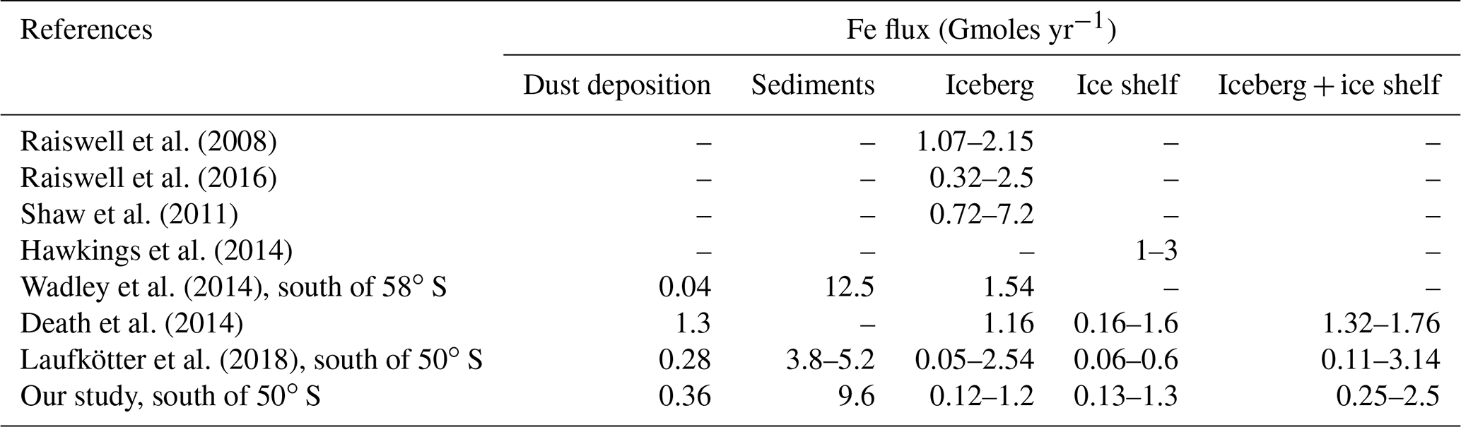
The iceberg-hosted sediment content, while poorly constrained by observations, is estimated to range from 0.4 to 1.2 g L−1 (Anderson et al., 1980; Shaw et al., 2011). To simulate the Fe fluxes delivered by melting icebergs and ice shelves in the SO, we associate with the freshwater flux climatologies a sediment content of 0.5 g L−1 as used in Raiswell et al. (2006) and Death et al. (2014) assuming, as a crude assumption, that sediment content in icebergs and ice shelves is roughly equivalent. The content of ferrihydrite, the most soluble Fe in iceberg-hosted sediments and thus potentially bioavailable, has been recently estimated to range from 0.03 wt % to 0.194 wt % with a mean content of 0.076 wt % (Raiswell et al., 2016). Shaw et al. (2011) estimated a range of ferrihydrite of 0.04 wt % to 0.4 wt % for free-drifting icebergs in the Weddell Sea. In our study, we set the mean sediment content in ferrihydrite to be 0.1 %. A conservative value of the fraction of ferrihydrite that can be biologically available as Fe nanoparticles (i.e., the soluble fraction of ferrihydrite) is around 10 % (Raiswell et al., 2008; Death et al., 2014). However, ice–water–mineral reactions may profoundly alter the bioavailability percentage of Fe in glacial sediments (Hawkings et al., 2018; Raiswell et al., 2010, 2018). In order to account for the uncertainty of the bioavailable fraction of glacial Fe (Boyd et al., 2012; Raiswell et al., 2010, 2018), we use a solubility within a range of 1 % to 10 %, which corresponds to a total annual Fe flux of 0.25 to 2.5 Gmoles yr−1 (Table 1). The range of the modeled iceberg Fe fluxes is relatively similar to other modeling studies (Death et al., 2014; Laufkötter et al., 2018) and lies within the lower range of previously published estimates based on observations (Raiswell et al., 2008, 2016; Shaw et al., 2011). To our knowledge, no observational data are available that allow ice shelf Fe fluxes from the AIS to be constrained. However, the modeled ice shelf Fe fluxes are in the lower range of estimates by Hawkings et al. (2014) for the AIS, as extrapolated from Greenland Ice Sheet data.
Raiswell et al. (2008)Raiswell et al. (2016)Shaw et al. (2011)Hawkings et al. (2014)Wadley et al. (2014)Death et al. (2014)Laufkötter et al. (2018)Table 1Annual estimates of Fe fluxes from observational and modeling studies in the SO. The iceberg Fe flux from Raiswell et al. (2016) is calculated by applying an Fe solubility of 10 % to their estimates of potentially bioavailable Fe fluxes.
2.3 Experimental design
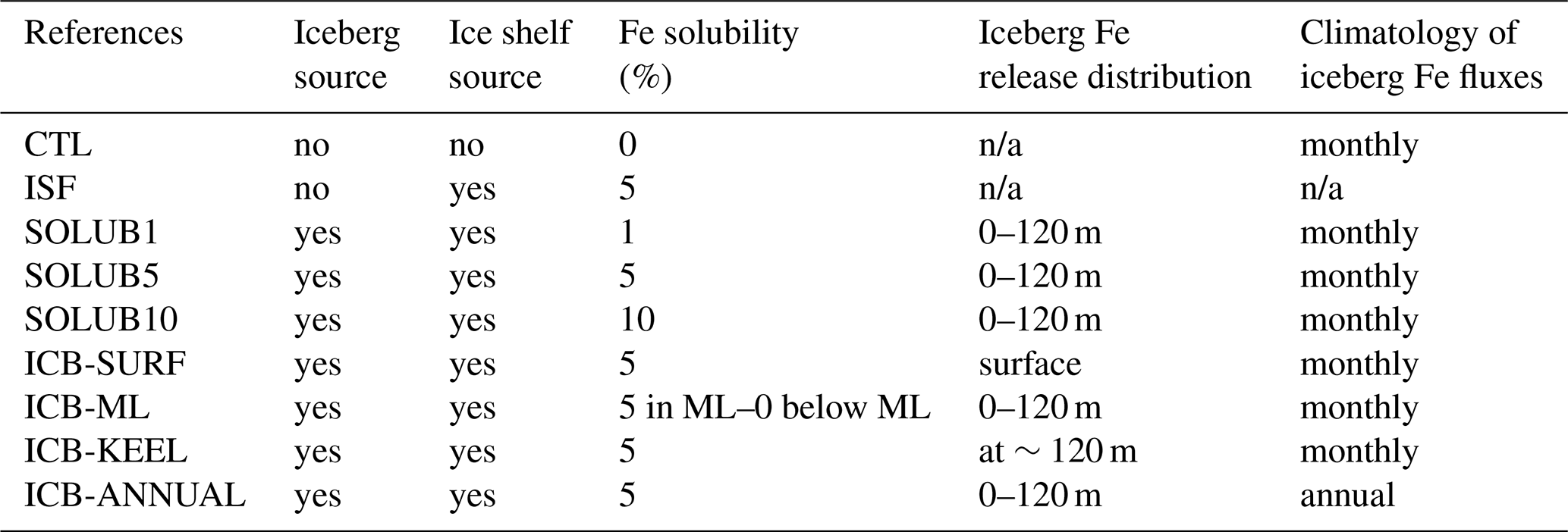
We design nine model experiments with different Fe solubilities for both ice shelves and icebergs, as well as different vertical distributions of delivered Fe from icebergs (Table 2). For consistency with the climatological forcing of the Antarctic freshwater release, all these experiments are run in a climatological setup using the CORE-I normal year atmospheric forcing (Griffies et al., 2009) and are initialized from a 120-year-long spin-up simulation. They all include external sources of Fe from dust, sediments, sea ice, and rivers even though the latter does not contribute to the iron pool in the SO. Each experiment is run for 20 years to achieve a sufficient equilibrium state for the Fe cycle in the framework of our sensitivity study.
Table 2Description of model experiments. The ice shelf Fe supply is uniformly distributed over the depth and width of the unresolved cavities, from the mean ice front base down to the seabed or the grounding line depth if shallower, following the parameterization of Mathiot et al. (2017). The climatology of ice shelf Fe fluxes is annual.
The control experiment (CTL) is used as a reference run in the rest of the study and does not take into account any Fe source from the AIS. Figure 2 shows the annual mean distribution of surface Fe concentrations over the SO simulated by the CTL experiment. This distribution is contrasted with regions showing high surface Fe concentrations in coastal regions around the Antarctic continent, in the surrounding waters of SO islands, such as South Georgia, the Crozet archipelago, and the Kerguelen Plateau, and with large areas in the open ocean displaying very low values. The modeled surface distribution of Fe concentrations reflects the main contribution of sediments among the different external iron sources currently implemented in the standard version of the PISCES model (Aumont et al., 2015). The Fe distribution of the NEMO-PISCES model has been validated at the global scale in Tagliabue et al. (2016) and over the SO in Person et al. (2018), showing reasonable performance compared to available data (Tagliabue et al., 2012).
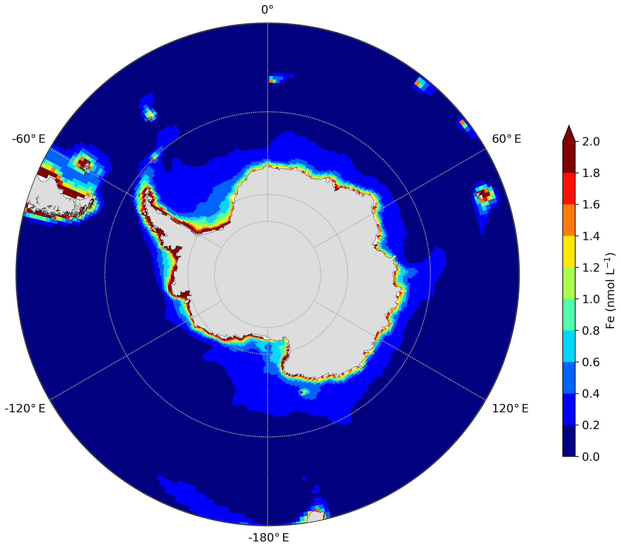
Figure 2Annual mean of surface Fe concentrations in the Southern Ocean, south of 45∘ S, in the CTL experiment.
Three different solubilities of Fe from icebergs and ice shelves are tested in the SOLUB1, SOLUB5, and SOLUB10 experiments, imposing 1 %, 5 %, and 10 %, respectively. The corresponding annual Fe fluxes amount to 0.25, 1.25, and 2.5 Gmoles yr−1, respectively, with similar contributions from both glacial sources (Table 1). The ISF, ICB-SURF, ICB-ML, ICB-KEEL, and ICB-ANNUAL experiments have an iceberg and ice shelf Fe solubility of 5 % as in the SOLUB5 experiment. The ISF experiment only includes the Fe source from ice shelves in order to assess its contribution relative to icebergs.
Different vertical distributions of the iceberg Fe fluxes are explored. In the SOLUB1, SOLUB5, SOLUB10, and ICB-ANNUAL experiments, Fe is homogeneously released from icebergs over the top 120 m of the water column. This value corresponds to the average depth of the submerged part of the five size classes of icebergs modeled by the NEMO-ICB model (Marsh et al., 2015) and computed by applying the formulation of Rackow et al. (2017) to the average thickness of the modeled icebergs. In the ICB-SURF experiment, the whole iceberg Fe supply is released at the surface, i.e., in the first vertical level of our model, which is 1 m thick. In the ICB-KEEL experiment, this flux is released at ∼120 m, i.e., at the mean depth of the keel of modeled icebergs. The ICB-KEEL experiment is set up to evaluate the contribution of a theoretical distribution of iceberg Fe fluxes delivered only at the base of icebergs. The ICB-KEEL experiment can be seen as the mirror experiment of the ICB-SURF experiment, keeping in mind that this distribution is most probably unrealistic as the potential buoyancy effect tends to upwell the iceberg meltwater to the surface (Smith et al., 2007; Helly et al., 2011; Stephenson et al., 2011). The different vertical distributions of iceberg Fe fluxes prescribed in our experiments offer an indirect means to explore the potential impact of that mechanism on ocean biogeochemistry. In order to evaluate the role played by the iceberg Fe fluxes distributed below the mixed layer (ML), that is, the fraction not directly available for surface primary productivity, we design the ICB-ML experiment in which this fraction is removed. Thus, the iceberg Fe fluxes in the ICB-ML experiment are distributed throughout the water column, i.e., until a depth of 120 m, as in the SOLUB5 experiment, but the iceberg Fe flux values below the mixed layer depth (MLD) are set to zero unlike in the SOLUB5 experiment. Finally, in the ICB-ANNUAL experiment, an annual mean climatology of the iceberg Fe fluxes is used instead of the monthly climatology to assess the impact of the seasonal variability in the supply of Fe from icebergs in the SO.
3.1 Contribution of the Antarctic Ice Sheet to the spatial distribution of Fe
3.1.1 Sensitivity to the magnitude of the Antarctic Ice Sheet Fe supply
The uncertainty in the magnitude of the AIS Fe source is estimated to span at least 1 order of magnitude (Table 1). We assess the impact of this range on the spatial distribution of Fe in the SO by imposing three different soluble fractions of Fe: 1 %, 5 %, and 10 % (Table 2). The Fe supply from the AIS increases the Fe concentrations in the first 120 m in the SOLUB1, SOLUB5, and SOLUB10 experiments compared to the CTL experiment, respectively, and the surface anomaly increases with the Fe solubility (Fig. 3).
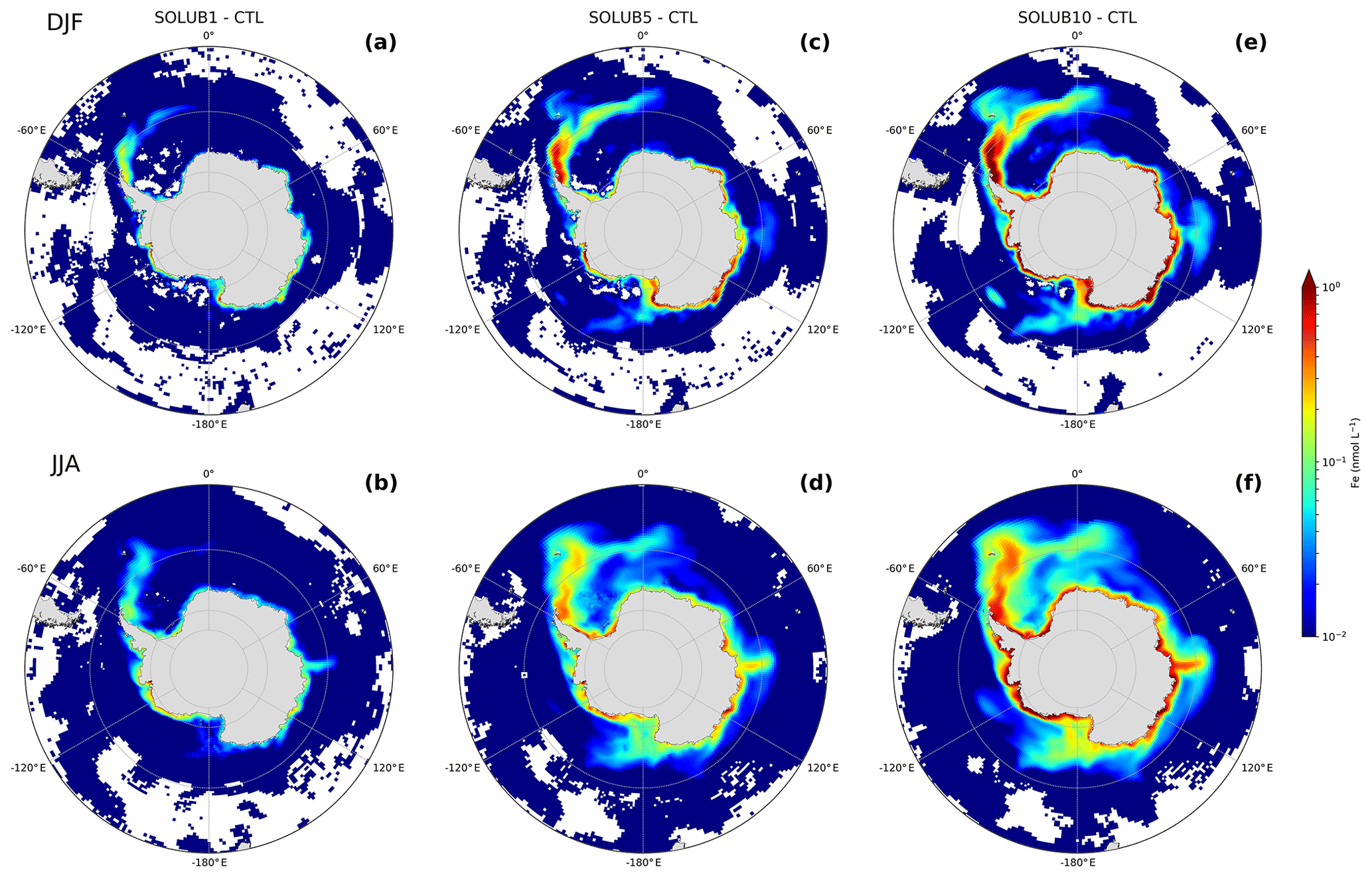
Figure 3Difference in surface Fe concentrations between the (a, b) SOLUB1, (c, d) SOLUB5, and (e, f) SOLUB10 experiments and the CTL experiment (experiments minus CTL) in (a, c, e) summer (December, January, and February) and (b, d, f) winter (June, July, and August) in the Southern Ocean, south of 45∘ S. White areas are regions with nonsignificant changes. Note the logarithmic scale.
Higher surface Fe concentrations are simulated in coastal regions all around the Antarctic continent. The most noticeable Fe anomaly is a marked plume northeast of the Antarctic Peninsula that expands until 50∘ S in the Atlantic sector and reaches the western sector of the Indian Ocean (Fig. 3c–f). The spatial extent of the Fe anomalies becomes larger as the Fe solubility increases, particularly in the Atlantic sector and in the Ross Sea, which appear to be the offshore areas that are the most greatly influenced by the AIS Fe source. The SOLUB1 experiment simulates a moderate impact with annual mean surface Fe concentrations increased by ∼0.026 nmol L−1 over the SO, south of 50∘ S, relative to the CTL experiment, i.e., 3 % more. The supply in the Atlantic plume increases the surface Fe concentrations by up to 0.16 nmol L−1 in summer (Fig. 3a). The highest Fe values are found in winter along the coasts of the Ross Sea and the Amundsen Sea with surface Fe anomalies that reach 1 nmol L−1 (Fig. 3b). In the SOLUB5 experiment, the contribution of the AIS Fe source is more significant, with mean surface Fe concentrations that are ∼0.12 nmol L−1 higher, i.e., 13 % more than in the CTL experiment (Fig. 3c and d). The Atlantic plume is clearly marked and extends further eastward until 10∘ E with surface Fe concentrations in summer up to ∼0.8 nmol L−1 higher (Fig. 3c). Along the Antarctic coast, the AIS supply in winter increases the surface Fe anomalies by up to 3.8 nmol L−1, particularly in the Indian and Pacific sectors (Fig. 3d). Two additional plumes emerge: a large one north of the Ross Sea and a smaller one in the vicinity of South Georgia (Fig. 3c and d). The SOLUB10 experiment strengthens the seasonal and spatial patterns of the surface Fe anomalies simulated in SOLUB5 with extensive Fe anomalies in the Atlantic plume, in the Ross Sea, in the Weddell Sea, and all along the Antarctic coast (Fig. 3e and f). Over the SO, south of 50∘ S, the annual mean Fe concentrations are ∼0.21 nmol L−1 higher than in the CTL experiment, an increase of 24 %. The surface Fe concentrations in the Atlantic plume and along the Antarctic coast are up to ∼1.4 and ∼6.3 nmol L−1 higher, respectively. These Fe concentrations are difficult to compare to observations in these areas due to the scarcity of data. However, they are probably at the upper limit of Fe concentrations in the open ocean but still potentially realistic in coastal regions (de Jong et al., 2012). With an Fe solubility of 10 %, the SOLUB10 experiment predicts an important contribution of the AIS source to the SO Fe pool (Fig. 3e), which is even larger near the coasts in winter (Fig. 3f).
The AIS significantly alters the surface Fe concentrations both in summer and winter (Fig. 3). The spatial patterns between these two seasons exhibit noticeable differences. In summer, surface Fe anomalies are marked and intense (Fig. 3c and e), whereas in winter they extend over larger areas and are more diffuse (Fig. 3d and f), showing lower maximum values but having higher mean levels. These seasonal differences reflect two different dynamics in the supply of Fe from the AIS and its subsequent loss from the surface. In summer, the release of Fe associated with more intense iceberg freshwater fluxes drives surface Fe concentrations to high values. Environmental conditions are favorable for phytoplankton growth and the intense biological activity efficiently consumes the supplied Fe, preventing it from being transported over large distances, especially in iron-limited areas. In winter, biological activity is much weaker due to strong light limitation and the delivered Fe from the AIS can be advected further away. Furthermore, in winter, deep mixing entrains to the surface Fe that was released in summer below the euphotic zone and that escaped consumption by phytoplankton due to the lack of light. This unconsumed fraction is also advected over significant distances by the intense ocean circulation in the SO. This explains the much sharper gradients simulated in summer, particularly noticeable in the SOLUB5 and SOLUB10 experiments.
3.1.2 Sensitivity to vertical distributions of the iceberg Fe supply
It is well established that ice shelf meltwater is injected at depth into the ocean (Depoorter et al., 2013; Mathiot et al., 2017). The basal melting is driven by the properties of water masses that enter the ocean cavities underneath ice shelves (Jacobs et al., 1992), contributing directly and indirectly to the supply of Fe to the upper layer of the water column (St-Laurent et al., 2017, 2019). While the iceberg Fe supply has been evidenced by in situ observations (Lin et al., 2011; Shaw et al., 2011; De Jong et al., 2015), almost nothing is known to our knowledge about where the Fe delivery occurs along the immersed part of icebergs and where this input is predominately available to phytoplankton. Nonetheless, FitzMaurice et al. (2017) recently pointed out that the nonlinear response of iceberg melting leads to meltwater injected near the surface or mixed at depth depending on whether the flow velocity is weak or strong, respectively. Here, we assess the impacts of four different theoretical vertical distributions of iceberg Fe fluxes on surface Fe concentrations over the SO as well as on vertical profiles of Fe in the upper 300 m of a large area highly fertilized by the AIS northeast of the Antarctic Peninsula (36–56∘ W, 58–63∘ S). For this purpose, we compare the ICB-SURF, ICB-ML, and ICB-KEEL experiments against the SOLUB5 experiment (Fig. 4).

Figure 4Difference in surface Fe concentrations between the (a, b) ICB-SURF, (c, d) ICB-ML, (e, f) ICB-KEEL, and (g, h) ICB-ANNUAL experiments and the SOLUB5 experiment (experiments minus SOLUB5) in (a, c, e, g) summer (December, January, and February) and (b, d, f, h) winter (June, July, and August) in the Southern Ocean, south of 45∘ S. Positive values in red are regions with surface Fe concentrations higher than in the SOLUB5 experiment, and negative values in blue are regions with surface Fe concentrations lower than in the SOLUB5 experiment.
The surface distribution of the iceberg Fe fluxes in the ICB-SURF experiment results in a large excess of surface Fe concentrations in summer compared to the volume distribution applied in the SOLUB5 experiment (Fig. 4a). This excess is regionally important, with surface Fe concentrations up to 1.5 nmol L−1 higher in the large plume of the Atlantic sector and up to 27 nmol L−1 higher in coastal areas than in the SOLUB5 experiment. Such maximum coastal concentrations of surface Fe are rarely observed except in a nearshore area north of the Antarctic Peninsula (de Jong et al., 2012). In the ICB-SURF experiment, the iceberg Fe supply in the mixed layer is maximum and is not sensitive to the depth of the mixed layer. By contrast, when the Fe flux is distributed over the upper 120 m (SOLUB5), the shallow pycnocline in summer severely limits the iceberg Fe supply in the mixed layer, with most of this supply being injected below the MLD. The differences between the two experiments in winter are significantly less marked, with large patterns of positive and negative differences in surface Fe concentrations highlighting the role played by the interactions between the seasonal variations of the MLD and the injection of Fe at depth (Fig. 4b). When the MLD is deeper than 120 m, the ICB-SURF experiment simulates slightly lower Fe concentrations up to ∼0.04 nmol L−1 lower than in SOLUB5 in the Atlantic sector south of 60∘ S and regionally around the Antarctic coast. The boundary zone between positive and negative values in the Atlantic sector is driven by the interplay between an MLD shallower than 120 m (Fig. 5) and the oceanic circulation, resulting in Fe concentrations up to 1.5 nmol L−1 higher in the ICB-SURF experiment than in SOLUB5 along the eastern coasts of the Antarctic Peninsula. Higher Fe concentrations are also simulated in ICB-SURF in localized areas in the Ross, Amundsen, and Bellingshausen seas, as well as near the coasts of the Indian sector between 70 and 85∘ E but without a clear correlation with the MLD.

Figure 5Difference in surface Fe concentrations between the ICB-SURF and the SOLUB5 experiments in winter (June, July, and August) in the Southern Ocean, south of 45∘ S. The black isoline represents the mixed layer depth at 120 m, and the gray isolines represent mixed layer depth shallower than 120 m.
The vertical profiles of Fe in the highly fertilized area of the Atlantic plume northeast of the Antarctic Peninsula (36–56∘ W, 58–63∘ S) illustrate the different dynamic in the seasonal supply of Fe to the upper ocean in both experiments (Fig. 6). In summer, these vertical profiles are very different (Fig. 6a). In the mixed layer, Fe concentrations are higher in ICB-SURF than in SOLUB5 by a factor of 2.2. Below the MLD, the ICB-SURF experiment simulates Fe concentrations that decrease strongly until 70 m. In the SOLUB5 experiment, Fe concentrations increase significantly from below 30 until 120 m and from there decrease until 150 m. Below 150 m, both experiments converge to the same vertical profile of Fe. In winter, the vertical profiles are qualitatively similar in the upper 300 m (Fig. 6b). Yet, the ICB-SURF experiment displays a smaller vertical gradient in the upper 150 m than in SOLUB5. The scarcity of data makes it challenging to discriminate whether the ICB-SURF experiment or the SOLUB5 experiment simulates a realistic vertical distribution of Fe.
The ICB-ML experiment permits the assessment of the influence of the iceberg Fe supplied below the MLD, i.e., the importance of the nondirectly available fraction of the iceberg Fe source, on the spatial distribution of Fe over the SO. Surface Fe concentrations in the ICB-ML experiment are lower than in the SOLUB5 experiment in both seasons and over the whole SO (Fig. 4c and d). Surface Fe values in summer and winter are up to ∼0.55 and ∼0.4 nmol L−1 lower, respectively, than in the SOLUB5 experiment. This comparison suggests that the Fe fraction delivered by icebergs below the MLD is not completely scavenged and constitutes an Fe pool that can supply surface waters with Fe as soon as the mixed layer deepens.
The seasonal evolution of the vertical Fe profiles supports the important role of the subsurface additional pool of Fe due to iceberg melting (Fig. 6). In summer, the SOLUB5 experiment has Fe concentrations in the mixed layer ∼0.1 nmol L−1 higher than in the ICB-ML experiment (Fig. 6a). Below the MLD, Fe concentrations in SOLUB5 display a local maximum between 30 and 150 m that the ICB-ML experiment does not simulate. In winter, Fe profiles in SOLUB5 and ICB-ML are qualitatively similar except that Fe levels in ICB-ML are about 0.06 nmol L−1 higher (Fig. 6b). This comparison illustrates that the Fe released by icebergs in summer below the MLD may represent a significant subsurface reservoir that can supply Fe to the surface layer through intraseasonal events such as storms (Swart et al., 2015; Nicholson et al., 2016), strong mesoscale and sub-mesoscale activities (Swart et al., 2015; Rosso et al., 2016), and deep mixing in winter (Tagliabue et al., 2014b).
The iceberg Fe supply at depth in the ICB-KEEL experiment shows a significant decrease in surface Fe concentrations compared to the SOLUB5 experiment in both seasons (Fig. 4e and f). In summer, surface Fe concentrations are up to ∼2.8 nmol L−1 lower than in the SOLUB5 experiment in the Atlantic plume and all around the Antarctic coast (Fig. 4e). In winter, the difference is weaker than in summer, with surface Fe concentrations up to ∼0.8 nmol L−1 lower than in the SOLUB5 experiment (Fig. 4f). Moreover, the spatial differences between the two experiments in the open ocean in winter are less widespread than in the ICB-ML experiment (Fig. 4d) in which the iceberg fertilization effect is less effective south of the Atlantic plume and, more generally, south of 60∘ S offshore of the Antarctic coast. While low, the supply of Fe from icebergs at depth can have a large area of influence on surface Fe concentrations in winter.
The vertical profile of Fe in the Atlantic plume presents a marked peak at a depth of 120 m, which corresponds to the depth at which Fe is released from iceberg melting. At this depth, Fe concentrations reach 1.2 nmol L−1 in summer, which is 0.5 nmol L−1 higher than in the SOLUB5 experiment (Fig. 6a). In the upper layer, Fe concentrations are lower by ∼0.2 nmol L−1 than in the SOLUB5 experiment and almost equal to the CTL experiment. The vertical gradient is the strongest of all the experiments. In winter, surface Fe concentrations in the mixed layer are ∼0.09 nmol L−1 lower than in the SOLUB5 experiment and slightly higher than in the CTL experiment (Fig. 6b). The vertical gradient between the surface and 120 m remains stronger than in any other experiments but the difference is weaker. Below 120 m and down to about 200 m, differences with the other experiments are significantly smaller than in summer. These results show that a predominant supply of Fe at the base of icebergs will generate an important subsurface reservoir of Fe that can be entrained to the surface by the deepening of the MLD. The role of the subsurface reservoir of Fe is pointed out to be critical to sustain the iron supply to surface waters (Tagliabue et al., 2014b).

Figure 6Vertical profiles of Fe concentrations until 300 m northeast of the Antarctic Peninsula (36–56∘ W, 58–63∘ S) in the CTL (blue), SOLUB5 (red), ICB-ML (green), ICB-KEEL (gray), ICB-ANNUAL (pink), and ICB-SURF (orange) experiments in (a) summer (December, January, and February) and in (b) winter (June, July, and August). The solid light gray line is the mixed layer depth (MLD) in (a) summer and (b) winter averaged over the region, in gray shading is the standard deviation of the MLD over the region in (a) summer and (b) winter, and the dashed gray line is the 120 m isobath.
3.1.3 Sensitivity to the seasonal variations of the iceberg Fe supply
The variations of the AIS Fe fluxes due to the seasonal variability of iceberg calving and melting (Fig. 1a) impact the seasonal cycle of Fe over the SO. To assess to what extent these variations are significant for the SO Fe pool, we compare the ICB-ANNUAL experiment to the SOLUB5 experiment. Over the whole SO, the surface Fe concentrations in the ICB-ANNUAL experiment and the SOLUB5 experiment are increased by 9 % and 13 % in summer and by 15 % and 13 % in winter, respectively, relative to the CTL experiment. Imposing an annual mean iceberg supply of Fe also leads to differences in the spatial distribution of Fe (Fig. 4g and h). In ICB-ANNUAL, surface Fe concentrations in summer are lower in the Atlantic sector and around the Antarctic coast than in the SOLUB5 experiment, with values up to ∼1.9 nmol L−1 lower (Fig. 4g). On the other hand, some other areas such as downstream of South Georgia, in the Weddell Sea, and in the Ross Sea are predicted to have higher Fe concentrations. In the Weddell Sea, along the east coasts of the Antarctic Peninsula, the Fe values in the ICB-ANNUAL experiment are up to 0.2 nmol L−1 higher than in the SOLUB5 experiment. In winter, an opposite spatial pattern is simulated (Fig. 4h). Surface Fe concentrations in the Atlantic plume and along the east coasts are up to ∼0.75 nmol L−1 higher in the ICB-ANNUAL experiment, whereas downstream of South Georgia, in the Weddell Sea, in the Ross Sea, and offshore of 80∘ E these concentrations are up to ∼0.45 nmol L−1 lower. When looking at the vertical Fe distribution in the Atlantic plume, vertical profiles in summer have almost the same shape in both experiments (Fig. 6a). However, Fe concentrations in ICB-ANNUAL are lower by ∼0.1 nmol L−1 in the upper 120 m than in SOLUB5. In winter, the vertical profile of Fe in ICB-ANNUAL is noticeably different, with Fe concentrations higher by ∼0.18 nmol L−1 in the upper 50 m and with values that increase and then decrease by ∼0.1 nmol L−1 between 50 and 150 m, whereas Fe concentrations in the SOLUB5 experiment increase gradually in this depth range (Fig. 6b). Thus, when the seasonal variations of iceberg Fe are not considered, the seasonal amplitude of the Fe cycle over the SO is increased, with Fe concentrations higher in winter and lower in summer (Fig. S2a), leading to significant regional differences in the surface distribution of Fe.
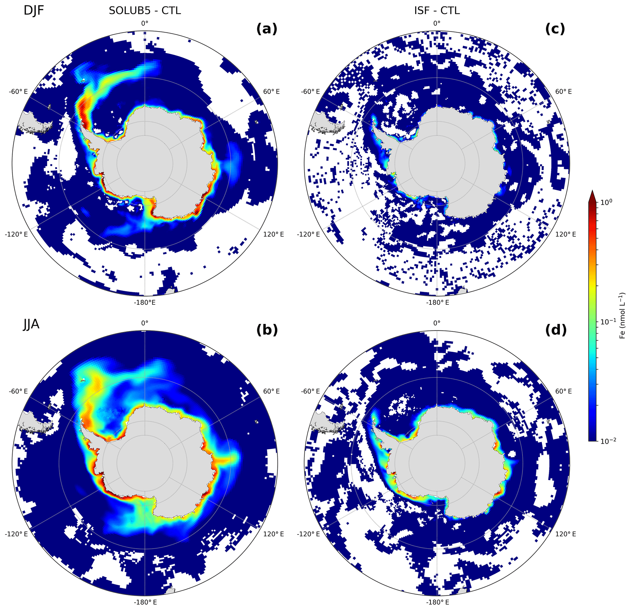
Figure 7Difference in surface Fe concentrations between the (a, b) SOLUB5 and (c, d) ISF experiments and the CTL experiment (experiments minus CTL) in (a, c) summer (December, January, and February) and (b, d) winter (June, July, and August) in the Southern Ocean, south of 45∘ S. White areas are regions with nonsignificant changes. Note the logarithmic scale.
3.1.4 Evaluation of the ice shelf contribution
The AIS Fe supply occurs through two main processes: (1) the basal melting of ice shelves, which is coastal, and (2) the calving and melting of icebergs, which is more widespread over the SO. Both freshwater sources are estimated to be of the same order of magnitude (Depoorter et al., 2013). In addition, ice shelf melting contributes indirectly to the supply of Fe to the upper layer of the water column through the meltwater pump driven by the buoyancy overturning circulation near the ice shelf fronts (St-Laurent et al., 2017, 2019). The relative contribution of each source of Fe to the SO iron pool is not known, mainly due to the lack of data for ice shelves. Here, we compare the ISF experiment, which only accounts for the ice shelf Fe source, against the SOLUB5 experiment, which encompasses both sources of Fe from the AIS. The surface Fe anomalies in the ISF experiment differ remarkably from the SOLUB5 experiment (Fig. 7). The ice shelf contribution is trapped near the Antarctic coast, extending further offshore in winter (Fig. 7c and d), whereas the spatial contribution of icebergs spreads the influence of the AIS Fe source more widely over the SO until 50∘ S (Fig. 7a and b).
The surface Fe concentrations in the ISF experiment are increased by 1 % and 3 % compared to the CTL experiment in summer and winter, respectively. The contribution of ice shelves to the SO Fe pool is 1 order of magnitude lower than in the SOLUB5 experiment, which simulates surface Fe concentrations that are increased by 13 % in both seasons. The comparison between the two Fe sources highlights the higher fertilization capacity of icebergs due to a delivery at larger spatial scales. It also suggests that the direct and indirect supplies of Fe to surface waters from ice shelf melting are significantly limited by the stratification of the mixed layer. Moreover, the ice shelf supply occurs in coastal regions already highly fertilized by sediments and where elevated Fe concentrations experience intense scavenging. The additional Fe from ice shelves is therefore rapidly scavenged and lost from surface waters.
3.2 Fertilization effect of the Antarctic Ice Sheet on surface chlorophyll
The SO is the largest HNLC region where Fe is the main limiting micronutrient for primary productivity. We show that the Fe supply by ice shelf and iceberg melting can fertilize the surface waters all year round (Fig. 3). This additional input of Fe can be used at the blooming season by phytoplankton from November to February. Here, we qualitatively evaluate the fertilization effect of the AIS on surface chlorophyll concentrations (SChl) in summer (December, January, and February). First of all, we briefly compare the SChl climatology from satellite observations of the MODIS Aqua ocean color product estimated by Johnson et al. (2013) to the CTL experiment (Fig. 8a and b). At the scale of the SO, two main qualitative characteristics can be observed. The CTL experiment represents with a rather good approximation the SChl distribution in summer around the Antarctic continent, from the Antarctic coast until 65∘ S. But, in the open ocean north of 65∘ S, quite large differences between observations and the standard version of the model are seen, especially in the Atlantic sector and in the Pacific sector north of the Ross Sea where large spatial patterns of SChl are not simulated.
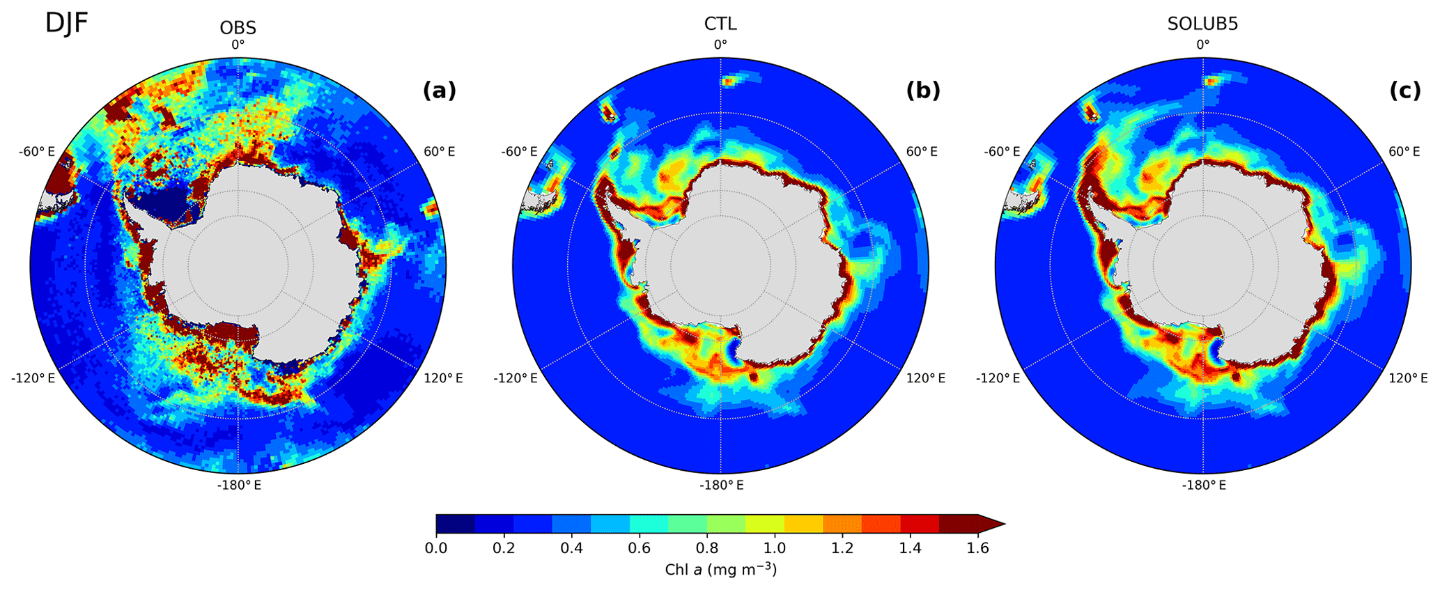
Figure 8Surface chlorophyll concentrations in summer (December, January, and February) from (a) satellite observations (MODIS Aqua; Johnson et al., 2013), (b) the CTL experiment, and (c) the SOLUB5 experiment in the Southern Ocean, south of 50∘ S.
To assess the fertilization effect of the AIS on SChl, we compute the SChl difference between the eight experiments and the CTL experiment (Fig. 9). The AIS impact on SChl is mostly apparent in the Atlantic sector northeast of the Antarctic Peninsula, along the Antarctic coast in the Indian and Pacific sectors, and, more moderately, north of the Ross Sea. The fertilization effect increases with the Fe solubility, with SChl higher by 2 %, 7 %, and 12 % in the SOLUB1, SOLUB5, and SOLUB10 experiments, respectively (Fig. 9a–c). The main features driven by the intensity of the AIS Fe source are the extension of an Atlantic plume until the Indian sector and the increased SChl along the coasts from 80∘ E until the Ross Sea. In the SOLUB1 experiment, the impact on SChl is particularly low, restricted to the Atlantic sector and in coastal areas around 135∘ E (Fig. 9a). The Atlantic plume has the smallest extent from the Antarctic Peninsula until the South Orkney Islands where SChl values are up to ∼0.4 mg m−3 higher than in the CTL experiment. The Fe solubility of 5 % implemented in the SOLUB5 experiment significantly increases the impact of the AIS on SChl (Fig. 9b). The Atlantic plume extends eastward, far from the Antarctic Peninsula and the South Orkney Islands. The blooms along the Antarctic coast in the eastern sector and in the Ross Sea get more intense, and two modest plumes emerge north of the Ross Sea and around 90∘ E. The maximum contribution to SChl between the Antarctic Peninsula and the South Orkney Islands is ∼1 mg m−3 higher than in the CTL experiment and 2.2 mg m−3 higher in the coastal area around 135∘ E. The SOLUB10 experiment emphasizes the spatial patterns described in the SOLUB5 experiment, with SChl higher by ∼1.2 mg m−3 in the Atlantic sector until Bouvet Island and up to ∼2.4 mg m−3 higher along the coasts in the eastern sector of the SO (Fig. 9c). The plume that extends northward from the Ross Sea until 60∘ S has more elevated SChl levels, about ∼0.3 mg m−3 higher than in the CTL experiment.
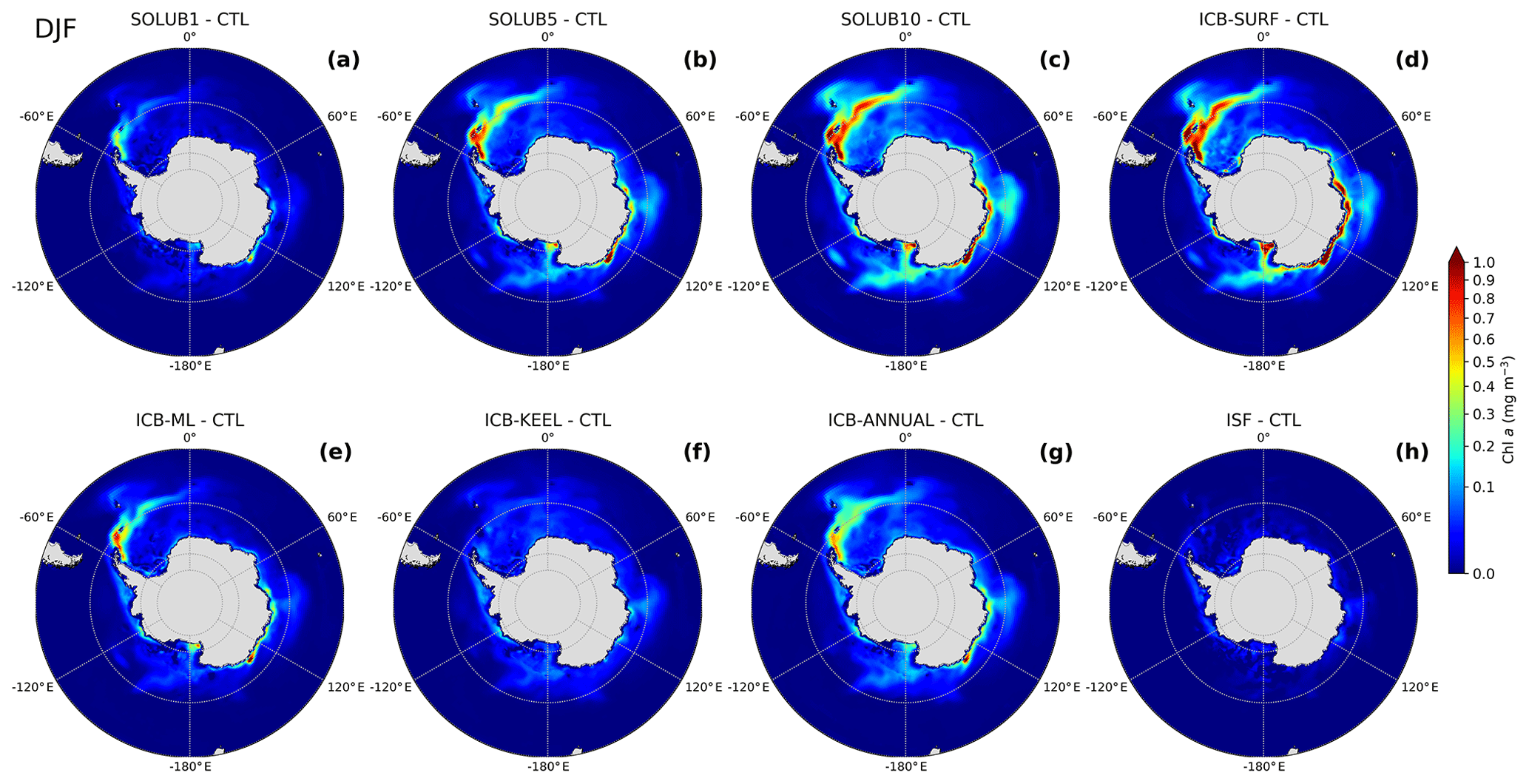
Figure 9Difference in surface chlorophyll concentrations in summer (December, January, and February) between the (a) SOLUB1, (b) SOLUB5, (c) SOLUB10, (d) ICB-SURF, (e) ICB-ML, (f) ICB-KEEL, (g) ICB-ANNUAL, and (h) ISF experiments and the CTL experiment (experiments minus CTL) in the Southern Ocean, south of 45∘ S.
In the ICB-SURF experiment, the simulated contribution to SChl is the largest, with an increase of 12 % over the whole SO. The maximum SChl values are up to ∼1.3 mg m−3 higher in the Atlantic plume and up to ∼2.5 mg m−3 higher in the Ross Sea and along the east coasts of Antarctica relative to the CTL experiment (Fig. 9d). Despite a slightly higher intensity of the bloom, the spatial patterns in the ICB-SURF experiment are very similar to the SOLUB10 experiment (Fig. 9c and d). In contrast, in the ICB-KEEL experiment, the iceberg contribution to surface chlorophyll is the lowest, SChl being on average only 2 % higher relative to CTL. The Atlantic plume is absent, as are the elevated concentrations along the Antarctic coast and in the Ross Sea (Fig. 9f). Nevertheless, though small, a fertilizing effect is simulated with SChl values that are locally higher by 0.25 mg m−3 than in the CTL experiment. The ICB-ML experiment produces SChl anomalies that lie between the SOLUB1 and the SOLUB5 experiments, with maximum SChl up to ∼0.9 and ∼1.6 mg m−3 higher than in the CTL experiment in the Atlantic plume and in local areas along the east coasts of Antarctica, respectively (Fig. 9e). The influenced area is clearly smaller than in the SOLUB5 experiment, demonstrating that the nondirectly available fraction of Fe delivered by melting icebergs may have a non-negligible impact on SChl during the blooming season. The ICB-ANNUAL experiment simulates SChl levels that are on average higher by 6 % over the SO compared to the CTL experiment with anomalies higher by ∼0.7 mg m−3 in the Atlantic plume and up to ∼1.2 mg m−3 along the Antarctic coast (Fig. 9g). Although maximum SChl values in the Atlantic plume are ∼0.3 mg m−3 lower, the simulated spatial extent of the SChl anomalies in the Atlantic sector is wider than in the SOLUB5 experiment, the other impacted areas being almost identical in the ICB-ANNUAL and the SOLUB5 experiments. In the ISF experiment, the increase in SChl is very small as a consequence of the weak impact of ice shelf melting on Fe (Fig. 9h, see Sect. 3.1.4).
3.3 Model evaluation
The purpose of this sensitivity study is not to specifically improve the skill of the biogeochemical model at representing the Fe and SChl distributions in the SO but to investigate the uncertainties associated with the external source of Fe from the AIS. However, in order to confirm that large biases are not introduced by the implementation of the new iron source in the biogeochemical model, we perform a statistical model–data comparison for Fe and SChl over the SO, south of 50∘ S. For Fe, we compare the model experiments to a global database constructed by Tagliabue et al. (2012). For surface chlorophyll concentrations, we use a monthly climatology of satellite-based (MODIS Aqua) estimates from Johnson et al. (2013). The statistical comparison shows that performance scores for annual Fe concentrations integrated over the upper 200 m and surface chlorophyll in summer are similar in all experiments (Tables S1 and S2 in the Supplement). The biases are relatively small, ranging from −0.07 to 0.02 nmol L−1 for Fe and −0.13 to −0.07 mg m−3 for SChl. The main difference is the increase in the mean Fe and surface chlorophyll concentrations showing a better agreement with observations, such as in the SOLUB5 experiment for Fe (Table S1) and in the SOLUB10 and ICB-SURF experiments for SChl (Table S2). This statistical analysis reveals no degradation of the performance skill of the standard version of the biogeochemical model when the AIS Fe source is added but also no improvements in the spatial distributions of Fe and chlorophyll concentrations. Thus, the absence of the AIS Fe fluxes is not a major cause that explains the biased representation of Fe and SChl in the NEMO-PISCES model.
3.4 Contribution of the Antarctic Ice Sheet to primary production and carbon export
At the blooming season, the Fe supply from the AIS stimulates phytoplankton activity, which can be quantified in terms of primary production and carbon (C) export. The increase in the annual primary production of phytoplankton (diatoms and nanophytoplankton) integrated over depth is relatively low in the Fe solubility experiments compared to the total primary production of 2.39 PgC yr−1 computed over the SO, south of 50∘ S, in the CTL experiment (Table 3). The increase in primary production ranges from 0.01 PgC yr−1 in the SOLUB1 experiment to 0.12 PgC yr−1 in the SOLUB10 experiment, i.e., a difference of 1 order of magnitude between the least and the most impacted cases. In the SOLUB10 experiment, primary production is 5 % higher than in the CTL experiment, a difference that drops to less than 1 % in the SOLUB1 experiment. This slightly enhanced primary productivity increases C export by 1 % in the SOLUB1 experiment and by more than 8 % in the SOLUB10 experiment. With an Fe solubility of 5 %, primary production simulated in the SOLUB5 experiment is ∼3 % higher and C export around 5 % higher than in the CTL experiment. Thus, the supply of Fe from the AIS results in a non-negligible but modest increase in C export at the scale of the SO and subsequent sequestration of carbon in the interior of the ocean.
Table 3Annual primary production integrated over depth (PP) and C export at a depth of 150 m in the CTL experiment and in the AIS Fe source experiments over the Southern Ocean, south of 50∘ S. In brackets are the increases in PP and C export relative to the CTL experiment in the highly fertilized plume of the Atlantic sector, northeast of the Antarctic Peninsula (36–56∘ W, 58–63∘ S).

For the other sensitivity experiments, the predicted impacts on primary production and C export all fall between those simulated by the SOLUB1 and SOLUB10 experiments. Releasing Fe at the surface as tested in the ICB-SURF experiment produces changes that are only slightly lower than in the SOLUB10 experiment. This suggests that the efficiency of the AIS Fe source is higher when located at the surface. The comparison of the SOLUB5 experiment with the ICB-ML experiment reveals that the nondirectly available fraction of Fe released from icebergs may increase the impact of the source on primary production and C export by ∼40 %. The ICB-ANNUAL experiment shows a primary production and a C export almost equal to the SOLUB5 experiment, suggesting no effect of the seasonal variability of iceberg Fe supply on annual primary productivity and C export at the scale of the SO. Finally, when only the ice shelf Fe source is considered in the ISF experiment, primary production and C export are almost unchanged compared to the CTL experiment.
4.1 Sensitivity of Fe and chlorophyll to the iron source from the Antarctic Ice Sheet
Our sensitivity study aims to delineate the biogeochemical impacts of the uncertainties surrounding the fertilization capacity of the AIS. Different aspects of the AIS Fe fluxes are explored: the intensity of the source, the impact of the iceberg Fe distribution in the water column, and the contribution of the seasonal variations of the iceberg meltwater.
The Fe supply from the AIS is highly sensitive to the hypothesized solubility of ferrihydrite, revealing strong impacts on the spatial distribution of Fe. The main supply of Fe occurs in the Atlantic sector downstream of the Antarctic Peninsula, along the Antarctic coast, and, more moderately, in the Ross Sea. The iceberg contribution to surface Fe is large and can extend until 50∘ S, as shown by the large plume expanding from the Antarctic Peninsula until the Indian sector (Fig. 3). The spatial distribution of the surface Fe anomalies in our model setup is in line with Laufkötter et al. (2018) but differs substantially from Death et al. (2014). In Death et al. (2014), the main fertilized area is simulated along the eastern sector of the Antarctic coast, showing a larger offshore extent, the Atlantic plume is clearly much less marked and extended, and the AIS influence in the region of the Ross Sea is weaker. These differences may be linked to the implementation in Death et al. (2014) of basal iceberg sediment loading, which induces high Fe concentrations in the basal layer and very low concentrations above this basal layer, whereas a homogeneous distribution is considered in our study. Their vertically varying distribution of Fe in icebergs may simulate a stronger fertilization effect in the calving regions driven by an important basal melting. Further offshore, once the basal Fe-rich part of icebergs has melted, the release of Fe is strongly decreased due to the lower Fe concentrations in the upper part of icebergs, resulting in a weaker fertilization effect in remote areas of the open ocean such as in the Atlantic sector.
The AIS fertilization impact on surface chlorophyll depends on the intensity of the AIS Fe source as well as on the choice of its vertical distribution (Fig. 9). The efficiency of the fertilization is regionally important, with increased SChl along the east coasts of Antarctica and in the core of the Atlantic plume off the tip of the Antarctic Peninsula. However, at the scale of the SO, south of 50∘ S, the AIS impact on primary production is quite modest, reaching a maximum increase of 5 % in our set of experiments relative to the control run (Table 3). Our results are similar (lower by 3 %) to Wadley et al. (2014) but contrast sharply with the 30 % increase in primary production estimated in Death et al. (2014). The AIS contribution in Death et al. (2014) is evaluated against atmospheric dust, sediments being not taken into account. The lack of the sedimentary Fe source, estimated to be the largest in the SO (Lancelot et al., 2009; Tagliabue et al., 2009, 2014a; Borrione et al., 2014; Wadley et al., 2014), leads to a significant increase in the fertilization effect of icebergs and ice shelves, particularly in coastal regions where sediment supplies have a large influence. Our study suggests that the AIS fertilization effect is weaker than suggested by Death et al. (2014), especially in coastal areas, as a consequence of the large input of Fe from sediment remobilization.
The enhanced primary production increases the C export by 8.4 % in our most impacted case (Table 3), a result significantly lower than the increase in particle export of 30 % in Laufkötter et al. (2018). The reasons for such a difference are difficult to disentangle as the modeled Fe fluxes from the AIS, atmospheric dust, and sediments are the same order of magnitude between the two studies (Table 1). Potential differences in the two modeling setups may arise from a different treatment of sediment mobilization, in particular in the description of the horizontal and vertical distribution of sediments or from a different relationship between primary production and C export. Indeed, observations suggest that the C export efficiency declines significantly with increasing primary productivity in the SO, although the causes remain unclear (Maiti et al., 2013; Le Moigne et al., 2016). In our model, this relationship, highly variable at local and temporal scales, is not linear in the SO but has a clear trend wherein a higher primary productivity is associated with a higher C export (not shown). In the model used in Laufkötter et al. (2018), a different relationship could explain the differences in the C export. While low at the scale of the SO in our model, the fertilization effect of the AIS on primary productivity and C export can be regionally significant as estimated from data (Smith et al., 2007; Duprat et al., 2016; Herraiz-Borreguero et al., 2016; Wu and Hou, 2017). For instance, in the highly fertilized area of the Atlantic plume, northeast of the Antarctic Peninsula (36–56∘ W, 58–63∘ S), primary production and C export are increased by ∼30 % and ∼42 %, respectively, in the SOLUB10 experiment compared to the CTL experiment (Table 3), i.e., 5 to 6 times higher than at the scale of the whole SO.
Climatically our study points out that the fertilization effect of the AIS on C export is moderate on timescales of 50 to 100 years. However, when integrated over timescales of thousands of years, the role played by the AIS in carbon sequestration might be a key component alongside atmospheric dust iron for the glacial–interglacial regulation of the carbon cycle (Martin, 1990). In a climate change perspective, our results suggest that any change in the supply of Fe from increased melting of icebergs and ice shelves should result in a quite moderate impact on ocean biogeochemistry and export production at the scale of the whole SO. Indeed, doubling the AIS Fe fluxes in the SOLUB10 experiment increases the C export by only ∼3.6 % compared to the SOLUB5 experiment (Table 3). Nevertheless, at a more local scale, the fertilization effect of the AIS induced by global warming could be drastically strengthened, with potentially important consequences for phytoplankton physiology, nutrient availability, and marine ecosystems (Boyd et al., 2010b, 2015; Hopwood et al., 2017; Boyd, 2019).
The choice of the iceberg Fe source distribution leads to significant differences in the magnitude of the fertilization effect of the AIS. In the case of a surface distribution, the effect is maximum. All the Fe delivered by the iceberg meltwater flux to the mixed layer is available to sustain primary productivity in spring and summer and strongly affects the vertical profiles of Fe, particularly in highly fertilized areas (Fig. 6). This theoretical distribution may lead to an overestimated supply of Fe in summer when the mixed layer is highly stratified, particularly in the case of large icebergs, partially ignoring the specific role of the Fe delivered below the MLD. Antarctic icebergs have different shapes (Romanov et al., 2012) and size class categories (Silva et al., 2006; Tournadre et al., 2015, 2016) both evolving during their life cycle (Bouhier et al., 2018). Moreover, the sediment distribution within icebergs is highly heterogeneous (Raiswell et al., 2016; Hopwood et al., 2017). All these features combined with distinct regimes of iceberg melting (FitzMaurice et al., 2017) fully constrain the delivery of Fe through the water column and below the mixed layer. Thus, the inherently heterogeneous nature of icebergs and their temporal evolution is extremely difficult to consider and to implement in a model. The choice of a surface distribution might be inappropriate to represent the iceberg supply in the ocean but without any degree of certainty. In fact, measured vertical profiles of Fe concentrations around icebergs in the Bellingshausen Sea in summer (De Jong et al., 2015) and in the Weddell Sea in autumn (Lin et al., 2011) suggest that both the ICB-SURF and SOLUB5 experiments simulate vertical distributions of Fe that could be observed in the wake of melting icebergs. At least, based on future observations, the representation of the iceberg Fe source could be better constrained and parameterized in models.
While the iceberg freshwater fluxes vary monthly (Fig. 1a), the AIS contribution to the SO Fe pool is almost equally effective in summer and winter, mainly driven by the balance between high AIS Fe fluxes and phytoplankton consumption in summer and low AIS Fe fluxes and light limitation in winter. However, the seasonal variations of the iceberg Fe fluxes contribute to significant differences in the spatial distributions of Fe (Fig. 4g and h), which have small impacts on annual primary production and C export when integrated over the SO (Table 3). The spatial differences in surface chlorophyll are relatively modest in summer between the SOLUB5 and ICB-ANNUAL experiments. Nevertheless, the larger amplitude of the Fe cycle over the SO in the ICB-ANNUAL experiment (Fig. S2a) modulates the seasonality of surface chlorophyll during the growing season: the bloom initialization occurs earlier, the bloom apex in December is higher, and the bloom decay is faster from January to April (Fig. S2b). Thus, the monthly variations of the iceberg Fe supply alter the seasonal cycle of chlorophyll in the SO.
4.2 Model caveats and uncertainties
A surprising result that may be linked to a potential model deficiency is the absence of the iron fertilization effect in the very close vicinity of the Antarctic coast. This can be observed in the difference of SChl between the SOLUB5 experiment and the CTL experiment (Fig. 9b). In fact, none of the iceberg fertilization experiments show an increase in chlorophyll near the Antarctic shores (Fig. 9). This unexpected result is due to a strong and systematic nutrient limitation in summer simulated by the biogeochemical model (Fig. S1). The seasonal cycles of nutrients at a station near the shore of the Amundsen Sea (106∘ W, 75∘ S) in the CTL and SOLUB5 experiments display a marked limitation in NO3, PO4, and Si in January and February (Fig. S1a–c), whereas Fe is non-limiting (Fig. S1d). Nutrient limitation strongly affects SChl in both experiments, as shown by their similar seasonal cycles (Fig. S1e). Nutrient limitation may occur locally along the Antarctic coast; however, high levels of primary productivity in spring and summer are observed in large regions such as in the numerous coastal polynyas present in the SO (Arrigo and van Dijken, 2003; Arrigo et al., 2015). This possible biased behavior of our model may result from missing, misrepresented processes or sources that may supply macro-nutrients in the mixed layer such as the oceanic circulation in ice shelf cavities (Jacobs et al., 2011; Herraiz‐Borreguero et al., 2015; White et al., 2019) or the melting of ice shelf and ice sheet (Pritchard et al., 2012; Arrigo et al., 2015, 2017; Hawkings et al., 2015; Wadham et al., 2016; St-Laurent et al., 2017). Another process that can be advocated is the entrainment of nutrient-rich waters by subglacial discharge plumes induced by basal melting of grounded glaciers, a physical mixing process observed in the western Antarctic Peninsula (Cape et al., 2019) and for Greenland glaciers (Meire et al., 2017; Hopwood et al., 2018; Kanna et al., 2018).
We highlight that the distribution of the iceberg Fe fluxes below the MLD may represent a non-negligible fraction of bioavailable Fe for primary productivity. Indeed, the iceberg Fe delivery at depth in the SOLUB5 and ICB-KEEL experiments feeds a subsurface reservoir of Fe that can supply surface waters by the deepening of the MLD through subseasonal storms (Swart et al., 2015; Nicholson et al., 2016) or deep mixing (Tagliabue et al., 2014b). We suggest that this distribution of the iceberg Fe source has to be considered if implemented in biogeochemical models. However, in our sensitivity study, we only apply one average depth of the submerged part of icebergs, whereas several size classes coexist in the SO where large tabular to small icebergs are observed covering a size range of 0.1–10 000 km2 (Tournadre et al., 2015, 2016; Silva et al., 2006). The size evolution of icebergs along their life cycle is poorly documented, but fragmentation is a significant mechanism in the reduction of their size, which increases the iceberg melt (Bouhier et al., 2018). This process impacts the temporal delivery of bioavailable Fe that we have not explored. Moreover, the distribution of the iceberg Fe fluxes in the water column, i.e., around and below icebergs, is probably not homogeneous as reported in De Jong et al. (2015) and Lin et al. (2011), giving an additional uncertainty not investigated here. Another uncertainty relates to the rates of Fe utilization released from melting icebergs along their drift that is estimated to be far less than that potentially supplied (Boyd et al., 2012). The assessment of this utilization is unfortunately impossible because of the contributions from other sources of Fe (sediments and dust). Furthermore, the Fe utilization is computed from satellite-derived net primary production that is associated with large uncertainties (Saba et al., 2011) and significant underestimates of surface chlorophyll in the SO (Johnson et al., 2013).
A large uncertainty in the fertilization capacity of Fe delivered by icebergs and ice shelves comes from the intrinsic nature of this sedimentary source. Indeed, a very large fraction of Fe found in icebergs has a lithogenic origin (Raiswell et al., 2006; Shaw et al., 2011). The supply of lithogenic Fe can be separated into three categories: the most soluble Fe, and thus potentially bioavailable, the semi-labile particulate Fe that will not dissolve rapidly once released to seawater, and the refractory insoluble fraction. We focused our study on the first fraction. However, the semi-labile fraction may have a significant contribution to fertilizing the surface waters of the SO. If lithogenic Fe with a low dissolution rate is not scavenged or experiences low sinking speeds (nanoparticles), this fraction can be maintained in the upper layer and become bioavailable on long timescales. This residence time may strongly affect the dissolved iron distribution from icebergs over the SO. As particulate lithogenic Fe is a significant pool of Fe in icebergs (Raiswell et al., 2006; Raiswell, 2011; Shaw et al., 2011), the contribution of the nondirectly bioavailable fraction to surface dissolved iron can be higher than actually observed. However, nothing is known about the fraction of lithogenic Fe bioavailable at long timescales or its quantity.
We implement in the biogeochemical model NEMO-PISCES (Aumont et al., 2015) the external source of iron from the Antarctic Ice Sheet based on recent estimates of Antarctic meltwater fluxes from icebergs and ice shelves (Depoorter et al., 2013; Merino et al., 2016). The modeled Fe fluxes from the AIS are in the range of previous modeling studies (Death et al., 2014; Laufkötter et al., 2018) and in the lower range of recent estimates from data (Raiswell et al., 2016). The potential indirect supply of Fe by the ice shelf melt-driven circulation, i.e., the meltwater pump (St-Laurent et al., 2017, 2019), is also represented by using the parameterization of Mathiot et al. (2017). We investigate the impacts of different sources of uncertainties related to the AIS iron source on Fe and surface chlorophyll distributions: the solubility of Fe, the vertical distribution of the iceberg source, and its seasonal variability. Large differences in the fertilization effect of the AIS are ultimately attributable to varying Fe solubility (1 %–10 %), which is currently poorly constrained by observations (Boyd et al., 2012; Raiswell et al., 2010, 2018). The AIS Fe supply is significant in the Atlantic sector northeast of the Antarctic Peninsula and along the Antarctic coast, particularly in the eastern sector, with large implications for the magnitude of phytoplankton blooms. The surface Fe and chlorophyll concentrations are increased by 3 % to 24 % and by 2 % to 12 %, respectively, at the scale of the SO. The contribution of Fe released from ice shelves is restricted to coastal areas with limited impact on chlorophyll and primary productivity, whereas modeled Fe fluxes from ice shelves and icebergs are similar. Our results also underline the role played by the vertical distribution of the iceberg Fe source due to the potentially non-negligible contribution of Fe delivered below the MLD. This nondirectly available supply cannot be considered a lost fraction for primary production but as a subsurface reservoir. The variability of the AIS contribution to the SO Fe pool is strongly linked to the interplay between the seasonal variations of meltwater released from icebergs and the physical and biological processes that characterize the dynamics of the SO: light limitation, MLD variations, iron limitation, and Fe consumption by phytoplankton.
At the scale of the SO, the fertilization effect of the AIS on primary production, mainly driven by icebergs, is relatively weak but with a non-negligible contribution to C export. In the most contributive case, primary production (integrated over depth) and C export (at 150 m) are increased by 5 % and 8.4 %, respectively, compared to our control experiment. However, in highly fertilized regions in the Atlantic sector and along the Antarctic coast, the AIS impact is more important, with primary production and C export being increased by up to 30 % and 42 %, respectively. The magnitude of the C export simulated here is noticeably lower than the AIS Fe contribution to the marine particle export recently estimated to 30 % over the SO in Laufkötter et al. (2018). This large difference emphasizes the necessity to continue exploring the large uncertainties that encompass the AIS Fe source and to understand the mechanisms that explain the very different sensitivity of C export to the AIS Fe fluxes simulated by models. Our results also point out the need to pursue in situ observations to better constrain the distribution of Fe and meltwater throughout the water column in the close vicinity of icebergs, their sediment content, and the range of Fe bioavailability from the AIS. Representing the biogeochemical features of the SO in ocean models is particularly challenging. However, we argue that the implementation of the external source of Fe from the AIS may help to fill the gap of misrepresented regional characteristics and to better represent the complexity of the SO iron cycle (Boyd and Ellwood, 2010; Tagliabue et al., 2017). Given that the Antarctic continental ice sheet has experienced a significant reduction of its mass (The IMBIE team, 2018) that may continue and amplify in the near future (Rintoul et al., 2018), it could be particularly relevant to integrate the AIS Fe source in climate models in order to assess its role for marine ecosystems and its potential negative feedbacks on climate change (Barnes et al., 2018). However, as there is currently limited agreement between models on the sensitivity of ocean biogeochemistry to the AIS Fe supply, the evaluation of climate change impacts on this external source of Fe and the consequences for marine biogeochemistry in the SO would be highly speculative.
The version code of the NEMO model, including PISCES-v2, used for this study is freely available at https://www.nemo-ocean.eu/ (last access: 18 September 2019). To access the NEMO svn repository, users should register on the NEMO website at https://forge.ipsl.jussieu.fr/nemo/register (last access: 18 September 2019). Model data are available at https://doi.org/10.5281/zenodo.2633097 (Person, 2019).
The supplement related to this article is available online at: https://doi.org/10.5194/bg-16-3583-2019-supplement.
The author contributions to this paper are as follows. RP and OA developed the conceptualization. RP conducted the formal analysis. OA and LB acquired funding. All authors contributed to the investigation. RP, OA, and GM prepared the methodology. RP and OA conducted the validation. RP completed the visualization and wrote the original first draft. All authors contributed to the review and final version.
The authors declare that they have no conflict of interest.
This work was performed using HPC resources from GENCI-IDRIS (grant 2018-A0040107451). The corrected ocean color product was retrieved from Australia's Integrated Marine Observing System (http://imos.org.au/, last access: 18 September 2019). The dissolved iron database is available on the GEOTRACES International Data Assemble Centre (https://www.bodc.ac.uk/geotraces/data/historical/, last access: 18 September 2019). We would like to thank Robert Raiswell and two anonymous referees for their helpful comments on the paper.
This research has been supported by the ANR SOBUMS (grant no. ANR-16-CE01-0014) and the EU-H2020-CRESCENDO (grant no. 641816).
This paper was edited by Tina Treude and reviewed by Robert Raiswell and two anonymous referees.
Anderson, J., Domack, E., and Kurtz, D.: Observations of Sediment–laden Icebergs in Antarctic Waters: Implications to Glacial Erosion and Transport, J. Glaciol., 25, 387–396, https://doi.org/10.3189/S0022143000015240, 1980. a
Arrigo, K. R. and van Dijken, G. L.: Phytoplankton dynamics within 37 Antarctic coastal polynya systems, J. Geophys. Res., 108, C8, https://doi.org/10.1029/2002JC001739, 2003. a
Arrigo, K. R., van Dijken, G. L., and Strong, A. L.: Environmental controls of marine productivity hot spots around Antarctica, J. Geophys. Res.-Oceans, 120, 5545–5565, https://doi.org/10.1002/2015JC010888, 2015. a, b
Arrigo, K. R., Dijken, G. L. V., Castelao, R. M., Luo, H., Rennermalm, A. K., Tedesco, M., Mote, T. L., Oliver, H., and Yager, P. L.: Melting glaciers stimulate large summer phytoplankton blooms in southwest Greenland waters, Geophys. Res. Lett., 44, 6278–6285, https://doi.org/10.1002/2017GL073583, 2017. a
Aumont, O., Ethé, C., Tagliabue, A., Bopp, L., and Gehlen, M.: PISCES-v2: an ocean biogeochemical model for carbon and ecosystem studies, Geosci. Model Dev., 8, 2465–2513, https://doi.org/10.5194/gmd-8-2465-2015, 2015. a, b, c, d
Barnes, D. K. A., Fleming, A., Sands, C. J., Quartino, M. L., and Deregibus, D.: Icebergs, sea ice, blue carbon and Antarctic climate feedbacks, Philos. T. R. Soc. A, 376, 20170176, https://doi.org/10.1098/rsta.2017.0176, 2018. a
Biddle, L. C., Kaiser, J., Heywood, K. J., Thompson, A. F., and Jenkins, A.: Ocean glider observations of iceberg-enhanced biological production in the northwestern Weddell Sea, Geophys. Res. Lett., 42, 459–465, https://doi.org/10.1002/2014GL062850, 2015. a, b
Blain, S., Quéguiner, B., Armand, L., Belviso, S., Bombled, B., Bopp, L., Bowie, A., Brunet, C., Brussaard, C., Carlotti, F., Christaki, U., Corbière, A., Durand, I., Ebersbach, F., Fuda, J.-L., Garcia, N., Gerringa, L., Griffiths, B., Guigue, C., Guillerm, C., Jacquet, S., Jeandel, C., Laan, P., Lefèvre, D., Lo Monaco, C., Malits, A., Mosseri, J., Obernosterer, I., Park, Y.-H., Picheral, M., Pondaven, P., Remenyi, T., Sandroni, V., Sarthou, G., Savoye, N., Scouarnec, L., Souhaut, M., Thuiller, D., Timmermans, K., Trull, T., Uitz, J., van Beek, P., Veldhuis, M., Vincent, D., Viollier, E., Vong, L., and Wagener, T.: Effect of natural iron fertilization on carbon sequestration in the Southern Ocean, Nature, 446, 1070–1074, https://doi.org/10.1038/nature05700, 2007. a
Blanke, B. and Delecluse, P.: Variability of the tropical Atlantic Ocean simulated by a general circulation model with two different mixed-layer physics, J. Phys. Oceanogr., 23, 1363–1388, 1993. a
Borrione, I., Aumont, O., Nielsdóttir, M. C., and Schlitzer, R.: Sedimentary and atmospheric sources of iron around South Georgia, Southern Ocean: a modelling perspective, Biogeosciences, 11, 1981–2001, https://doi.org/10.5194/bg-11-1981-2014, 2014. a, b, c
Bouhier, N., Tournadre, J., Rémy, F., and Gourves-Cousin, R.: Melting and fragmentation laws from the evolution of two large Southern Ocean icebergs estimated from satellite data, The Cryosphere, 12, 2267–2285, https://doi.org/10.5194/tc-12-2267-2018, 2018. a, b
Bowie, A. R., Maldonado, M. T., Frew, R. D., Croot, P. L., Achterberg, E. P., Mantoura, R. F. C., Worsfold, P. J., Law, C. S., and Boyd, P. W.: The fate of added iron during a mesoscale fertilisation experiment in the Southern Ocean, Deep-Sea Res. Pt. II, 48, 2703–2743, 2001. a
Boyd, P., Dillingham, P., McGraw, C., Armstrong, E., Cornwall, C., Feng, Y.-y., Hurd, C., Gault-Ringold, M., Roleda, M., Timmins-Schiffman, E., and Nunn, B.: Physiological responses of a Southern Ocean diatom to complex future ocean conditions, Nat. Clim. Change, 6, 2, https://doi.org/10.1038/nclimate2811, 2015. a
Boyd, P. W.: Physiology and iron modulate diverse responses of diatoms to a warming Southern Ocean, Nature Clim. Change, 9, 148–152, https://doi.org/10.1038/s41558-018-0389-1, 2019. a
Boyd, P. W. and Ellwood, M. J.: The biogeochemical cycle of iron in the ocean, Nat. Geosci., 3, 675–682, https://doi.org/10.1038/ngeo964, 2010. a
Boyd, P. W., Jickells, T., Law, C. S., Blain, S., Boyle, E. A., Buesseler, K. O., Coale, K. H., Cullen, J. J., de Baar, H. J. W., Follows, M., Harvey, M., Lancelot, C., Levasseur, M., Owens, N. P. J., Pollard, R., Rivkin, R. B., Sarmiento, J., Schoemann, V., Smetacek, V., Takeda, S., Tsuda, A., Turner, S., and Watson, A. J.: Mesoscale Iron Enrichment Experiments 1993-2005: Synthesis and Future Directions, Science, 315, 612–617, https://doi.org/10.1126/science.1131669, 2007. a, b
Boyd, P. W., Mackie, D., and Hunter, K.: Aerosol iron deposition to the surface ocean – Modes of iron supply and biological responses, Mar. Chem., 120, 128–143, https://doi.org/10.1016/j.marchem.2009.01.008, 2010a. a
Boyd, P. W., Strzepek, R., Fu, F., and Hutchins, D. A.: Environmental control of open-ocean phytoplankton groups: Now and in the future, Limnol. Oceanogr., 55, 1353–1376, https://doi.org/10.4319/lo.2010.55.3.1353, 2010b. a
Boyd, P. W., Arrigo, K. R., Strzepek, R., and van Dijken, G. L.: Mapping phytoplankton iron utilization: Insights into Southern Ocean supply mechanisms, J. Geophys. Res., 117, C6, https://doi.org/10.1029/2011JC007726, 2012. a, b, c, d
Cape, M. R., Vernet, M., Pettit, E. C., Wellner, J., Truffer, M., Akie, G., Domack, E., Leventer, A., Smith, C. R., and Huber, B. A.: Circumpolar Deep Water Impacts Glacial Meltwater Export and Coastal Biogeochemical Cycling Along the West Antarctic Peninsula, Front. Mar. Sci., 6, 144, https://doi.org/10.3389/fmars.2019.00144, 2019. a, b, c
Coale, K. H., Johnson, K. S., Chavez, F. P., Buesseler, K. O., Barber, R. T., Brzenski, M. A., Cochlan, W. P., Millero, F. J., Falkowski, P. G., Bauer, J. E., Wanninkhof, R. H., Kudela, R. M., Altabet, M. A., Hales, B. E., Takahashi, T., Landry, M. R., Bidigare, R. R., Wang, X., Chase, Z., Strutton, P. G., Friederich, G. E., Gorbunov, M. Y., Lance, V. P., Hilting, A. K., Hiscock, M. R., Demarest, M., and Hiscock, W. T.: Southern Ocean Iron Enrichment Experiment: Carbon Cycling in High- and Low-Si Waters, Science, 304, 408–414, https://doi.org/10.1126/science.1089778, 2004. a
de Baar, H. J. W., de Jong, J. T. M., Bakker, D. C. E., Löscher, B. M., Veth, C., Bathmann, U., and Smetacek, V.: Importance of iron for plankton blooms and carbon dioxide drawdown in the Southern Ocean, Nature, 373, 412–415, https://doi.org/10.1038/373412a0, 1995. a
de Jong, J., Schoemann, V., Lannuzel, D., Croot, P., de Baar, H., and Tison, J.-L.: Natural iron fertilization of the Atlantic sector of the Southern Ocean by continental shelf sources of the Antarctic Peninsula, J. Geophys. Res.-Biogeosci., 117, G1, https://doi.org/10.1029/2011JG001679, 2012. a, b
de Jong, J., Schoemann, V., Maricq, N., Mattielli, N., Langhorne, P., Haskell, T., and Tison, J.-L.: Iron in land-fast sea ice of McMurdo Sound derived from sediment resuspension and wind-blown dust attributes to primary productivity in the Ross Sea, Antarctica, Mar. Chem., 157, 24–40, https://doi.org/10.1016/j.marchem.2013.07.001, 2013. a
De Jong, J., Stammerjohn, S., Ackley, S., Tison, J.-L., Mattielli, N., and Schoemann, V.: Sources and fluxes of dissolved iron in the Bellingshausen Sea (West Antarctica): The importance of sea ice, icebergs and the continental margin, Mar. Chem., 177, 518–535, https://doi.org/10.1016/j.marchem.2015.08.004, 2015. a, b, c, d
Death, R., Wadham, J. L., Monteiro, F., Le Brocq, A. M., Tranter, M., Ridgwell, A., Dutkiewicz, S., and Raiswell, R.: Antarctic ice sheet fertilises the Southern Ocean, Biogeosciences, 11, 2635–2643, https://doi.org/10.5194/bg-11-2635-2014, 2014. a, b, c, d, e, f, g, h, i, j, k, l, m, n
DeConto, R. M. and Pollard, D.: Contribution of Antarctica to past and future sea-level rise, Nature, 531, 591–597, https://doi.org/10.1038/nature17145, 2016. a
Depoorter, M. A., Bamber, J. L., Griggs, J. A., Lenaerts, J. T. M., Ligtenberg, S. R. M., van den Broeke, M. R., and Moholdt, G.: Calving fluxes and basal melt rates of Antarctic ice shelves, Nature, 502, 89–92, https://doi.org/10.1038/nature12567, 2013. a, b, c, d, e
Dulaiova, H., Ardelan, M. V., Henderson, P. B., and Charette, M. A.: Shelf-derived iron inputs drive biological productivity in the southern Drake Passage, Global Biogeochem. Cy., 23, 4, https://doi.org/10.1029/2008GB003406, 2009. a
Duprat, L. P. A. M., Bigg, G. R., and Wilton, D. J.: Enhanced Southern Ocean marine productivity due to fertilization by giant icebergs, Nat. Geosci., 9, 219–221, https://doi.org/10.1038/ngeo2633, 2016. a, b, c
FitzMaurice, A., Cenedese, C., and Straneo, F.: Nonlinear response of iceberg side melting to ocean currents, Geophys. Res. Lett., 44, 5637–5644, https://doi.org/10.1002/2017GL073585, 2017. a, b
Gent, P. R. and McWilliams, J. C.: Isopycnal Mixing in Ocean Circulation Models, J. Phys. Oceanogr., 20, 150–155, 1990. a
Gerringa, L. J., Alderkamp, A.-C., Laan, P., Thuróczy, C.-E., De Baar, H. J., Mills, M. M., van Dijken, G. L., Haren, H. v., and Arrigo, K. R.: Iron from melting glaciers fuels the phytoplankton blooms in Amundsen Sea (Southern Ocean): Iron biogeochemistry, Deep-Sea Res. Pt. II, 71–76, 16–31, https://doi.org/10.1016/j.dsr2.2012.03.007, 2012. a, b
Griffies, S. M., Biastoch, A., Böning, C., Bryan, F., Danabasoglu, G., Chassignet, E. P., England, M. H., Gerdes, R., Haak, H., Hallberg, R. W., Hazeleger, W., Jungclaus, J., Large, W. G., Madec, G., Pirani, A., Samuels, B. L., Scheinert, M., Gupta, A. S., Severijns, C. A., Simmons, H. L., Treguier, A. M., Winton, M., Yeager, S., and Yin, J.: Coordinated Ocean-ice Reference Experiments (COREs), Ocean Modell., 26, 1–46, https://doi.org/10.1016/j.ocemod.2008.08.007, 2009. a
Hart, T.: On the phytoplankton of the south-west Atlantic and the Bellingshausen Sea, 1929–31, Discovery reports VIII, 1934. a
Hawkings, J. R., Wadham, J. L., Tranter, M., Raiswell, R., Benning, L. G., Statham, P. J., Tedstone, A., Nienow, P., Lee, K., and Telling, J.: Ice sheets as a significant source of highly reactive nanoparticulate iron to the oceans, Nat. Commun., 5, 3929, https://doi.org/10.1038/ncomms4929, 2014. a, b, c
Hawkings, J. R., Wadham, J., Tranter, M., Lawson, E., Sole, A., Cowton, T., Tedstone, A., Bartholomew, I., Nienow, P., Chandler, D., and Telling, J.: The effect of warming climate on nutrient and solute export from the Greenland Ice Sheet, Geochem. Perspect. Lett., 1, 94–104, https://doi.org/10.7185/geochemlet.1510, 2015. a
Hawkings, J. R., Benning, L. G., Raiswell, R., Kaulich, B., Araki, T., Abyaneh, M., Stockdale, A., Koch-Müller, M., Wadham, J. L., and Tranter, M.: Biolabile ferrous iron bearing nanoparticles in glacial sediments, Earth Planet. Sc. Lett., 493, 92–101, https://doi.org/10.1016/j.epsl.2018.04.022, 2018. a
Helly, J. J., Kaufmann, R. S., Stephenson, G. R., and Vernet, M.: Cooling, dilution and mixing of ocean water by free-drifting icebergs in the Weddell Sea, Deep-Sea Res. Pt. II, 58, 1346–1363, https://doi.org/10.1016/j.dsr2.2010.11.010, 2011. a, b
Herraiz-Borreguero, L., Lannuzel, D., van der Merwe, P., Treverrow, A., and Pedro, J. B.: Large flux of iron from the Amery Ice Shelf marine ice to Prydz Bay, East Antarctica, J. Geophys. Res.-Oceans, 121, 6009–6020, https://doi.org/10.1002/2016JC011687, 2016. a, b, c, d, e
Herraiz‐Borreguero, L., Coleman, R., Allison, I., Rintoul, S. R., Craven, M., and Williams, G. D.: Circulation of modified Circumpolar Deep Water and basal melt beneath the Amery Ice Shelf, East Antarctica, J. Geophys. Res.-Oceans, 120, 3098–3112, https://doi.org/10.1002/2015JC010697, 2015. a
Hodson, A., Nowak, A., Sabacka, M., Jungblut, A., Navarro, F., Pearce, D., Ávila Jiménez, M. L., Convey, P., and Vieira, G.: Climatically sensitive transfer of iron to maritime Antarctic ecosystems by surface runoff, Nat. Commun., 8, 14499, https://doi.org/10.1038/ncomms14499, 2017. a
Hooper, J., Mayewski, P., Marx, S., Henson, S., Potocki, M., Sneed, S., Handley, M., Gassó, S., Fischer, M., and Saunders, K. M.: Examining links between dust deposition and phytoplankton response using ice cores, Aeolian Res., 36, 45–60, https://doi.org/10.1016/j.aeolia.2018.11.001, 2019. a
Hopwood, M., Cantoni, C., Clarke, J., Cozzi, S., and Achterberg, E.: The heterogeneous nature of Fe delivery from melting icebergs, Geochem. Perspect. Lett., 3, 200–209, https://doi.org/10.7185/geochemlet.1723, 2017. a, b, c, d
Hopwood, M. J., Carroll, D., Browning, T. J., Meire, L., Mortensen, J., Krisch, S., and Achterberg, E. P.: Non-linear response of summertime marine productivity to increased meltwater discharge around Greenland, Nat. Commun., 9, 3256, https://doi.org/10.1038/s41467-018-05488-8, 2018. a
Ito, A., Myriokefalitakis, S., Kanakidou, M., Mahowald, N. M., Scanza, R. A., Hamilton, D. S., Baker, A. R., Jickells, T., Sarin, M., Bikkina, S., Gao, Y., Shelley, R. U., Buck, C. S., Landing, W. M., Bowie, A. R., Perron, M. M. G., Guieu, C., Meskhidze, N., Johnson, M. S., Feng, Y., Kok, J. F., Nenes, A., and Duce, R. A.: Pyrogenic iron: The missing link to high iron solubility in aerosols, Sci. Adv., 5, eaau7671, https://doi.org/10.1126/sciadv.aau7671, 2019. a
Jacobs, S. S., Helmer, H. H., Doake, C. S. M., Jenkins, A., and Frolich, R. M.: Melting of ice shelves and the mass balance of Antarctica, J. Glaciol., 38, 375–387, 1992. a
Jacobs, S. S., Jenkins, A., Giulivi, C. F., and Dutrieux, P.: Stronger ocean circulation and increased melting under Pine Island Glacier ice shelf, Nat. Geosci., 4, 519–523, https://doi.org/10.1038/ngeo1188, 2011. a
Johnson, R., Strutton, P. G., Wright, S. W., McMinn, A., and Meiners, K. M.: Three improved satellite chlorophyll algorithms for the Southern Ocean, J. Geophys. Res.-Oceans, 118, 3694–3703, https://doi.org/10.1002/jgrc.20270, 2013. a, b, c
Kanna, N., Sugiyama, S., Ohashi, Y., Sakakibara, D., Fukamachi, Y., and Nomura, D.: Upwelling of Macronutrients and Dissolved Inorganic Carbon by a Subglacial Freshwater Driven Plume in Bowdoin Fjord, Northwestern Greenland, J. Geophys. Res.-Biogeosci., 123, 1666–1682, https://doi.org/10.1029/2017JG004248, 2018. a
Khatiwala, S., Tanhua, T., Mikaloff Fletcher, S., Gerber, M., Doney, S. C., Graven, H. D., Gruber, N., McKinley, G. A., Murata, A., Ríos, A. F., and Sabine, C. L.: Global ocean storage of anthropogenic carbon, Biogeosciences, 10, 2169–2191, https://doi.org/10.5194/bg-10-2169-2013, 2013. a
Lancelot, C., de Montety, A., Goosse, H., Becquevort, S., Schoemann, V., Pasquer, B., and Vancoppenolle, M.: Spatial distribution of the iron supply to phytoplankton in the Southern Ocean: a model study, Biogeosciences, 6, 2861–2878, https://doi.org/10.5194/bg-6-2861-2009, 2009. a, b, c, d
Lannuzel, D., Schoemann, V., de Jong, J., Tison, J.-L., and Chou, L.: Distribution and biogeochemical behaviour of iron in the East Antarctic sea ice, Mar. Chem., 106, 18–32, https://doi.org/10.1016/j.marchem.2006.06.010, 2007. a
Lannuzel, D., Schoemann, V., de Jong, J., Pasquer, B., van der Merwe, P., Masson, F., Tison, J.-L., and Bowie, A.: Distribution of dissolved iron in Antarctic sea ice: Spatial, seasonal, and inter-annual variability, J. Geophys. Res., 115, G3, https://doi.org/10.1029/2009JG001031, 2010. a
Lannuzel, D., Vancoppenolle, M., van der Merwe, P., de Jong, J., Meiners, K., Grotti, M., Nishioka, J., and Schoemann, V.: Iron in sea ice: Review and new insights, Elementa, 4, 000130, https://doi.org/10.12952/journal.elementa.000130, 2016. a
Laufkötter, C., Stern, A. A., John, J. G., Stock, C. A., and Dunne, J. P.: Glacial Iron Sources Stimulate the Southern Ocean Carbon Cycle, Geophys. Res. Lett., 45, 13377–13385, https://doi.org/10.1029/2018GL079797, 2018. a, b, c, d, e, f, g, h, i, j
Le Moigne, F. A. C., Henson, S. A., Cavan, E., Georges, C., Pabortsava, K., Achterberg, E. P., Ceballos-Romero, E., Zubkov, M., and Sanders, R. J.: What causes the inverse relationship between primary production and export efficiency in the Southern Ocean?, Geophys. Res. Lett., 43, 4457–4466, https://doi.org/10.1002/2016GL068480, 2016. a
Lin, H., Rauschenberg, S., Hexel, C. R., Shaw, T. J., and Twining, B. S.: Free-drifting icebergs as sources of iron to the Weddell Sea, Deep-Sea Res. Pt. II, 58, 1392–1406, https://doi.org/10.1016/j.dsr2.2010.11.020, 2011. a, b, c, d, e, f, g
Madec, G.: NEMO ocean engine, Note du pole de modélisation de l'Institut Pierre-Simon Laplace, France, 27, 1–217, available at: http://epic.awi.de/39698/1/NEMO_book_v6039.pdf (last access: 18 September 2019), 2008. a, b, c, d
Maiti, K., Charette, M. A., Buesseler, K. O., and Kahru, M.: An inverse relationship between production and export efficiency in the Southern Ocean, Geophys. Res. Lett., 40, 1557–1561, https://doi.org/10.1002/grl.50219, 2013. a
Marsh, R., Ivchenko, V. O., Skliris, N., Alderson, S., Bigg, G. R., Madec, G., Blaker, A. T., Aksenov, Y., Sinha, B., Coward, A. C., Le Sommer, J., Merino, N., and Zalesny, V. B.: NEMO–ICB (v1.0): interactive icebergs in the NEMO ocean model globally configured at eddy-permitting resolution, Geosci. Model Dev., 8, 1547–1562, https://doi.org/10.5194/gmd-8-1547-2015, 2015. a, b, c
Martin, H, J., Fitzwater, E, S., and Gordon, R, M.: Iron Deficiency Limits Phytoplankton Growth in Antarctic Waters, Global Biogeochem. Cy., 4, 5–12, 1990. a
Martin, J. H.: Glacial‐interglacial CO2 change: The iron hypothesis, Paleoceanography, 5, 1–13, 1990. a, b
Mathiot, P., Jenkins, A., Harris, C., and Madec, G.: Explicit representation and parametrised impacts of under ice shelf seas in the z coordinate ocean model NEMO 3.6, Geosci. Model Dev., 10, 2849–2874, https://doi.org/10.5194/gmd-10-2849-2017, 2017. a, b, c, d
Meire, L., Mortensen, J., Meire, P., Juul‐Pedersen, T., Sejr, M. K., Rysgaard, S., Nygaard, R., Huybrechts, P., and Meysman, F. J. R.: Marine-terminating glaciers sustain high productivity in Greenland fjords, Global Change Biol., 23, 5344–5357, https://doi.org/10.1111/gcb.13801, 2017. a
Merino, N., Le Sommer, J., Durand, G., Jourdain, N. C., Madec, G., Mathiot, P., and Tournadre, J.: Antarctic icebergs melt over the Southern Ocean: Climatology and impact on sea ice, Ocean Modell., 104, 99–110, https://doi.org/10.1016/j.ocemod.2016.05.001, 2016. a, b, c, d
Nicholson, S.-A., Lévy, M., Llort, J., Swart, S., and Monteiro, P. M. S.: Investigation into the impact of storms on sustaining summer primary productivity in the Sub-Antarctic Ocean: Storms Sustain Summer Primary Production, Geophys. Res. Lett., 43, 9192–9199, https://doi.org/10.1002/2016GL069973, 2016. a, b
Person, R., Aumont, O., and Lévy, M.: The Biological Pump and Seasonal Variability of pCO2 in the Southern Ocean: Exploring the Role of Diatom Adaptation to Low Iron, J. Geophys. Res.-Oceans, 123, 5, https://doi.org/10.1029/2018JC013775, 2018. a
Person, R.: The Antarctic ice sheet iron source: a sensitivity study with a global ocean model, dataset, https://doi.org/10.5281/zenodo.2633097, 2019.
Pritchard, H. D., Ligtenberg, S. R. M., Fricker, H. A., Vaughan, D. G., van den Broeke, M. R., and Padman, L.: Antarctic ice-sheet loss driven by basal melting of ice shelves, Nature, 484, 502–505, https://doi.org/10.1038/nature10968, 2012. a
Rackow, T., Wesche, C., Timmermann, R., Hellmer, H. H., Juricke, S., and Jung, T.: A simulation of small to giant Antarctic iceberg evolution: Differential impact on climatology estimates, J. Geophys. Res.-Oceans, 122, 3170–3190, https://doi.org/10.1002/2016JC012513, 2017. a
Raiswell, R.: Iceberg-hosted nanoparticulate Fe in the Southern Ocean: Mineralogy, origin, dissolution kinetics and source of bioavailable Fe, Deep-Sea Res. Pt. II, 58, 1364–1375, https://doi.org/10.1016/j.dsr2.2010.11.011, 2011. a
Raiswell, R., Tranter, M., Benning, L. G., Siegert, M., De'ath, R., Huybrechts, P., and Payne, T.: Contributions from glacially derived sediment to the global iron (oxyhydr)oxide cycle: Implications for iron delivery to the oceans, Geochim. Cosmochim. Acta, 70, 2765–2780, https://doi.org/10.1016/j.gca.2005.12.027, 2006. a, b, c, d, e
Raiswell, R., Benning, L. G., Tranter, M., and Tulaczyk, S.: Bioavailable iron in the Southern Ocean: the significance of the iceberg conveyor belt, Geochem. Transact., 9, 1, https://doi.org/10.1186/1467-4866-9-7, 2008. a, b, c, d, e
Raiswell, R., Vu, H. P., Brinza, L., and Benning, L. G.: The determination of labile Fe in ferrihydrite by ascorbic acid extraction: Methodology, dissolution kinetics and loss of solubility with age and de-watering, Chem. Geol., 278, 70–79, https://doi.org/10.1016/j.chemgeo.2010.09.002, 2010. a, b, c
Raiswell, R., Hawkings, J. R., Benning, L. G., Baker, A. R., Death, R., Albani, S., Mahowald, N., Krom, M. D., Poulton, S. W., Wadham, J., and Tranter, M.: Potentially bioavailable iron delivery by iceberg-hosted sediments and atmospheric dust to the polar oceans, Biogeosciences, 13, 3887–3900, https://doi.org/10.5194/bg-13-3887-2016, 2016. a, b, c, d, e, f, g, h, i, j, k, l
Raiswell, R., Hawkings, J., Elsenousy, A., Death, R., Tranter, M., and Wadham, J.: Iron in Glacial Systems: Speciation, Reactivity, Freezing Behavior, and Alteration During Transport, Front. Earth Sci., 6, 222, https://doi.org/10.3389/feart.2018.00222, 2018. a, b, c
Rintoul, S. R., Chown, S. L., DeConto, R. M., England, M. H., Fricker, H. A., Masson-Delmotte, V., Naish, T. R., Siegert, M. J., and Xavier, J. C.: Choosing the future of Antarctica, Nature, 558, 233–241, https://doi.org/10.1038/s41586-018-0173-4, 2018. a, b, c
Romanov, Y. A., Romanova, N. A., and Romanov, P.: Shape and size of Antarctic icebergs derived from ship observation data, Antarctic Sci., 24, 77–87, https://doi.org/10.1017/S0954102011000538, 2012. a
Rosso, I., Hogg, A. M., Matear, R., and Strutton, P. G.: Quantifying the influence of sub-mesoscale dynamics on the supply of iron to Southern Ocean phytoplankton blooms, Deep-Sea Res. Pt. I, 115, 199–209, https://doi.org/10.1016/j.dsr.2016.06.009, 2016. a
Rousset, C., Vancoppenolle, M., Madec, G., Fichefet, T., Flavoni, S., Barthélemy, A., Benshila, R., Chanut, J., Levy, C., Masson, S., and Vivier, F.: The Louvain-La-Neuve sea ice model LIM3.6: global and regional capabilities, Geosci. Model Dev., 8, 2991–3005, https://doi.org/10.5194/gmd-8-2991-2015, 2015. a
Saba, V. S., Friedrichs, M. A. M., Antoine, D., Armstrong, R. A., Asanuma, I., Behrenfeld, M. J., Ciotti, A. M., Dowell, M., Hoepffner, N., Hyde, K. J. W., Ishizaka, J., Kameda, T., Marra, J., Mélin, F., Morel, A., O'Reilly, J., Scardi, M., Smith Jr., W. O., Smyth, T. J., Tang, S., Uitz, J., Waters, K., and Westberry, T. K.: An evaluation of ocean color model estimates of marine primary productivity in coastal and pelagic regions across the globe, Biogeosciences, 8, 489–503, https://doi.org/10.5194/bg-8-489-2011, 2011. a
Sabine, C. L., Feely, R. A., Gruber, N., Key, R. M., Lee, K., Bullister, J. L., Wanninkhof, R., Wong, C., Wallace, D. W., Tilbrook, B., Millero, F. J., Peng, T., Kozyr, A., Ono, T., and Rio, A. F.: The oceanic sink for anthropogenic CO2, science, 305, 367–371, 2004. a
Schwarz, J. and Schodlok, M.: Impact of drifting icebergs on surface phytoplankton biomass in the Southern Ocean: Ocean colour remote sensing and in situ iceberg tracking, Deep-Sea Res. Pt. I, 56, 1727–1741, https://doi.org/10.1016/j.dsr.2009.05.003, 2009. a
Shaw, T., Raiswell, R., Hexel, C., Vu, H., Moore, W., Dudgeon, R., and Smith, K.: Input, composition, and potential impact of terrigenous material from free-drifting icebergs in the Weddell Sea, Deep-Sea Res. Pt. II, 58, 1376–1383, https://doi.org/10.1016/j.dsr2.2010.11.012, 2011. a, b, c, d, e, f, g, h, i, j
Silva, T. A. M., Bigg, G. R., and Nicholls, K. W.: Contribution of giant icebergs to the Southern Ocean freshwater flux, J. Geophys. Res.-Oceans, 111, C3, https://doi.org/10.1029/2004JC002843, 2006. a, b
Smetacek, V.: EisenEx: international team conducts iron experiment in Southern Ocean, U.S. JGOFS Newsletter, 11, 11–14, 2001. a
Smith, K. L., Robison, B. H., Helly, J. J., Kaufmann, R. S., Ruhl, H. A., Shaw, T. J., Twining, B. S., and Vernet, M.: Free-Drifting Icebergs: Hot Spots of Chemical and Biological Enrichment in the Weddell Sea, Science, 317, 478–482, https://doi.org/10.1126/science.1142834, 2007. a, b, c, d
St-Laurent, P., Yager, P. L., Sherrell, R. M., Stammerjohn, S. E., and Dinniman, M. S.: Pathways and supply of dissolved iron in the Amundsen Sea (Antarctica), J. Geophys. Res.-Oceans, 122, 7135–7162, https://doi.org/10.1002/2017JC013162, 2017. a, b, c, d, e, f, g, h
St-Laurent, P., Yager, P. L., Sherrell, R. M., Oliver, H., Dinniman, M. S., and Stammerjohn, S. E.: Modeling the Seasonal Cycle of Iron and Carbon Fluxes in the Amundsen Sea Polynya, Antarctica, J. Geophys. Res.-Oceans, 124, 1544–1565, https://doi.org/10.1029/2018JC014773, 2019. a, b, c, d, e, f
Stephenson, G. R., Sprintall, J., Gille, S. T., Vernet, M., Helly, J. J., and Kaufmann, R. S.: Subsurface melting of a free-floating Antarctic iceberg, Deep-Sea Res. Pt. II, 58, 1336–1345, https://doi.org/10.1016/j.dsr2.2010.11.009, 2011. a, b
Swart, S., Thomalla, S., and Monteiro, P.: The seasonal cycle of mixed layer dynamics and phytoplankton biomass in the Sub-Antarctic Zone: A high-resolution glider experiment, J. Mar. Syst., 147, 103–115, https://doi.org/10.1016/j.jmarsys.2014.06.002, 2015. a, b, c
Tagliabue, A., Bopp, L., and Aumont, O.: Evaluating the importance of atmospheric and sedimentary iron sources to Southern Ocean biogeochemistry, Geophys. Res. Lett., 36, 13, https://doi.org/10.1029/2009GL038914, 2009. a, b, c, d
Tagliabue, A., Bopp, L., Dutay, J.-C., Bowie, A. R., Chever, F., Jean-Baptiste, P., Bucciarelli, E., Lannuzel, D., Remenyi, T., Sarthou, G., Aumont, O., Gehlen, M., and Jeandel, C.: Hydrothermal contribution to the oceanic dissolved iron inventory, Nat. Geosci., 3, 252–256, https://doi.org/10.1038/ngeo818, 2010. a
Tagliabue, A., Mtshali, T., Aumont, O., Bowie, A. R., Klunder, M. B., Roychoudhury, A. N., and Swart, S.: A global compilation of dissolved iron measurements: focus on distributions and processes in the Southern Ocean, Biogeosciences, 9, 2333–2349, https://doi.org/10.5194/bg-9-2333-2012, 2012. a, b
Tagliabue, A., Aumont, O., and Bopp, L.: The impact of different external sources of iron on the global carbon cycle, Geophys. Res. Lett., 41, 920–926, https://doi.org/10.1002/2013GL059059, 2014a. a, b
Tagliabue, A., Sallée, J.-B., Bowie, A. R., Lévy, M., Swart, S., and Boyd, P. W.: Surface-water iron supplies in the Southern Ocean sustained by deep winter mixing, Nat. Geosci., 7, 314–320, https://doi.org/10.1038/ngeo2101, 2014b. a, b, c
Tagliabue, A., Aumont, O., De'Ath, R., Dunne, J. P., Dutkiewicz, S., Galbraith, E., Misumi, K., Moore, J. K., Ridgwell, A., Sherman, E., Stock, C., Vichi, M., Völker, C., and Yool, A.: How well do global ocean biogeochemistry models simulate dissolved iron distributions?, Global Biogeochem. Cy., 30, 2, https://doi.org/10.1002/2015GB005289, 2016. a, b, c
Tagliabue, A., Bowie, A. R., Boyd, P. W., Buck, K. N., Johnson, K. S., and Saito, M. A.: The integral role of iron in ocean biogeochemistry, Nature, 543, 51–59, https://doi.org/10.1038/nature21058, 2017. a
The IMBIE team: Mass balance of the Antarctic Ice Sheet from 1992 to 2017, Nature, 558, 219–222, https://doi.org/10.1038/s41586-018-0179-y, 2018. a, b
Tournadre, J., Bouhier, N., Girard‐Ardhuin, F., and Rémy, F.: Large icebergs characteristics from altimeter waveforms analysis, J. Geophys. Res.-Oceans, 120, 1954–1974, https://doi.org/10.1002/2014JC010502, 2015. a, b
Tournadre, J., Bouhier, N., Girard-Ardhuin, F., and Rémy, F.: Antarctic icebergs distributions 1992-2014, J. Geophys. Res.-Oceans, 121, 327–349, https://doi.org/10.1002/2015JC011178, 2016. a, b
Wadham, J. L., Hawkings, J., Telling, J., Chandler, D., Alcock, J., O'Donnell, E., Kaur, P., Bagshaw, E., Tranter, M., Tedstone, A., and Nienow, P.: Sources, cycling and export of nitrogen on the Greenland Ice Sheet, Biogeosciences, 13, 6339–6352, https://doi.org/10.5194/bg-13-6339-2016, 2016. a
Wadley, M. R., Jickells, T. D., and Heywood, K. J.: The role of iron sources and transport for Southern Ocean productivity, Deep-Sea Res. Pt. I, 87, 82–94, https://doi.org/10.1016/j.dsr.2014.02.003, 2014. a, b, c, d, e, f
Wagener, T., Guieu, C., Losno, R., Bonnet, S., and Mahowald, N.: Revisiting atmospheric dust export to the Southern Hemisphere ocean: Biogeochemical implications, Global Biogeochem. Cy., 22, 2, https://doi.org/10.1029/2007GB002984, 2008. a
Wang, S., Bailey, D., Lindsay, K., Moore, J. K., and Holland, M.: Impact of sea ice on the marine iron cycle and phytoplankton productivity, Biogeosciences, 11, 4713–4731, https://doi.org/10.5194/bg-11-4713-2014, 2014. a
Wedepohl, K. H.: The composition of the continental crust, Geochim. Cosmochim. Acta, 59, 1217–1232, 1995. a
White, D. A., Fink, D., Post, A. L., Simon, K., Galton-Fenzi, B., Foster, S., Fujioka, T., Jeromson, M. R., Blaxell, M., and Yokoyama, Y.: Beryllium isotope signatures of ice shelves and sub-ice shelf circulation, Earth Planet. Sc. Lett., 505, 86–95, https://doi.org/10.1016/j.epsl.2018.10.004, 2019. a
Wu, S.-Y. and Hou, S.: Impact of icebergs on net primary productivity in the Southern Ocean, The Cryosphere, 11, 707–722, https://doi.org/10.5194/tc-11-707-2017, 2017. a, b