the Creative Commons Attribution 4.0 License.
the Creative Commons Attribution 4.0 License.
 | 31 Jul 2019
Sensitivity of atmospheric CO2 to regional variability in particulate organic matter remineralization depths
Jamie D. Wilson
Stephen Barker
Neil R. Edwards
Philip B. Holden
Andy Ridgwell
The concentration of CO2 in the atmosphere is sensitive to changes in the depth at which sinking particulate organic matter is remineralized: often described as a change in the exponent “b” of the Martin curve. Sediment trap observations from deep and intermediate depths suggest there is a spatially heterogeneous pattern of b, particularly varying with latitude, but disagree over the exact spatial patterns. Here we use a biogeochemical model of the phosphorus cycle coupled with a steady-state representation of ocean circulation to explore the sensitivity of preformed phosphate and atmospheric CO2 to spatial variability in remineralization depths. A Latin hypercube sampling method is used to simultaneously vary the Martin curve independently within 15 different regions, as a basis for a regression-based analysis used to derive a quantitative measure of sensitivity. Approximately 30 % of the sensitivity of atmospheric CO2 to changes in remineralization depths is driven by changes in the subantarctic region (36 to 60∘ S) similar in magnitude to the Pacific basin despite the much smaller area and lower export production. Overall, the absolute magnitude of sensitivity is controlled by export production, but the relative spatial patterns in sensitivity are predominantly constrained by ocean circulation pathways. The high sensitivity in the subantarctic regions is driven by a combination of high export production and the high connectivity of these regions to regions important for the export of preformed nutrients such as the Southern Ocean and North Atlantic. Overall, regionally varying remineralization depths contribute to variability in CO2 of between around 5 and 15 ppm, relative to a global mean change in remineralization depth. Future changes in the environmental and ecological drivers of remineralization, such as temperature and ocean acidification, are expected to be most significant in the high latitudes where CO2 sensitivity to remineralization is also highest. The importance of ocean circulation pathways to the high sensitivity in subantarctic regions also has significance for past climates given the importance of circulation changes in the Southern Ocean.
- Article
(4174 KB) -
Supplement
(2509 KB) - BibTeX
- EndNote


Sinking particles of organic matter transfer 5–10 Pg C per year from the upper ocean to the ocean interior (Henson et al., 2011) as part of a process known as the biological pump. As these particles sink, they are remineralized through bacterial- and zooplankton-related activity, releasing the carbon and nutrients back into solution at depth. Vertical fluxes of particulate organic carbon (POC) in the water column have historically been described by the Martin curve, a power-law function that describes the rapid decrease in flux (Fz) from a maximum value at depth z0, nominally the base of the mixed layer, to a small asymptotic value in deep waters (Fig. 1; Eq. 1; Martin et al., 1987):
The dimensionless exponent in the power law (b) describes whether organic matter is remineralized predominantly at shallower depths (larger values of b; e.g. b=1.6) or deeper in the water column (smaller values of b; e.g. b=0.4) (Fig. 1). The exponent itself parameterizes the rate at which POC sinks through the water column (units of m d−1) and the rate at which it is remineralized (units of d−1; Kriest and Oschlies, 2008; Lam et al., 2011). In this paper we use the term “remineralization depth”, defined as a depth at which a defined % of POC has been remineralized. Previously, this has been defined as an e folding depth: the depth at which ∼63 % of POC has been remineralized (Kwon et al., 2009; although note that the Martin curve is not exponential).
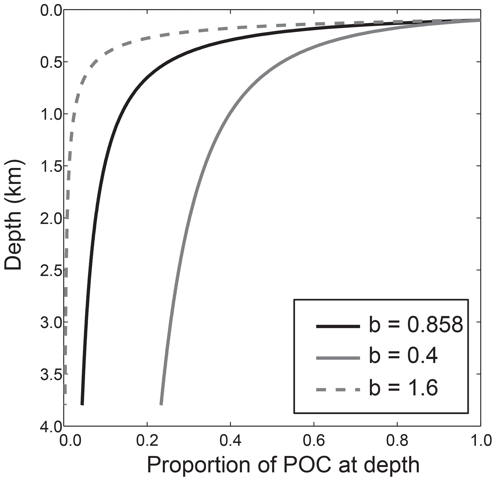
Figure 1The normalized water column distribution of particulate fluxes defined using the Martin curve. As a comparison, Martin curves are shown with the exponent found by Martin et al. (1987) (b=0.858) and minimum and maximum exponent values used in this study based on sediment trap data compilations (b=0.4, b=1.6; Henson et al., 2012; Marsay et al., 2015; Guidi et al., 2015). All curves have export depth (z0, Eq. 1) of 120 m.
Ocean biogeochemical models predict that the concentration of CO2 in the atmosphere is sensitive to changes in a globally uniform remineralization depth. Kwon et al. (2009) showed that a deepening of the remineralization depth globally of 24 m (from b=1.0 to 0.9) redistributed dissolved inorganic carbon (DIC) from the intermediate waters to the deep ocean, leading to a reduction in atmospheric CO2 of between 10 and 27 ppm. The drawdown was also associated with a decrease in the global mean concentration of preformed nutrients in the ocean interior (nutrients that are not utilised by biology in the surface ocean and enter the ocean interior via circulation; Ito and Follows, 2005). Kwon et al. (2009) found that an increase in respired carbon in the deep ocean was balanced by a reduction in preformed nutrients exported in the North Atlantic. Deepening of the POC remineralization depth could also drive dissolution of calcium carbonate (CaCO3) in ocean sediments, ultimately drawing down more CO2 over millennial timescales (Roth et al., 2014). The potential impact of remineralization depth changes on atmospheric CO2 is therefore a highly relevant component of the marine carbon cycle for both past and current changes in climate (Riebesell et al., 2009; Hülse et al., 2017; Meyer et al., 2016).
Analyses of global sediment trap observations suggest there is a spatially heterogeneous pattern of remineralization depths in the modern ocean that varies particularly with latitude. A synthesis of observations from deep sediment traps (>1500–2000 m; Henson et al., 2012) suggests that POC fluxes in high latitudes attenuate faster with depth (shallower remineralization depth: b=1.6) than in low latitudes, where a greater proportion of POC is transported to depth (deeper remineralization depth: b=0.4); see Fig. 1). However, POC fluxes measured using neutrally buoyant sediment traps at shallower depths (<1000 m) suggest the inverse of this latitudinal pattern (Marsay et al., 2015); see also Weber et al. (2016). A recent compilation of sediment trap data and profiles of particle size distributions observed in the water column highlight additional intra-basin variability in b (e.g. shallower remineralization in the eastern equatorial Pacific than in the western equatorial Pacific) and inter-basin variability (e.g. deeper remineralization in the Atlantic and Indian basins compared to the Pacific) (Guidi et al., 2015). The uncertainty in the spatial variability of remineralization depths presents a challenge for determining which mechanisms may be responsible for changes in remineralization depths and how these might drive future or past changes in remineralization (e.g. Boyd, 2015). Additionally, this also presents a challenge for biogeochemical models, which are beginning to resolve the mechanisms that are potentially responsible for these spatial patterns, such as particle-size-dependent sinking rates (DeVries et al., 2014), temperature-dependent remineralization (John et al., 2014), and oxygen dependence (Laufkötter et al., 2017).
A key question in light of the observed spatial variability in remineralization depths and the associated uncertainty in spatial patterns is what the sensitivity of atmospheric CO2 concentrations to spatial variability in remineralization depths is. Kwon et al. (2009) further quantified the sensitivity of atmospheric CO2 to basin-scale changes in remineralization depths by perturbing them in each basin individually, finding that the Pacific, Southern Ocean (defined as >40∘ S), Atlantic, and Indian oceans contributed 38 %, 22 %, 21 %, and 19 % of the total CO2 drawdown, respectively (Kwon et al., 2009). The variability in CO2 sensitivity between basins matched the variability in the magnitude of export production integrated over the basins and basin area, suggesting that no one region was more significant when varying the globally uniform remineralization depth (Kwon et al., 2009). However, this basin-scale analysis does not resolve the sensitivity of atmospheric CO2 occurring at the resolution suggested by observations, i.e. a latitudinal and within-basin scale, or at the resolution of ecological and biogeochemical variability (Longhurst, 1998; Fay and McKinley, 2014). Additionally, the analysis does not allow for the identification of potential interactions and feedbacks between regions when remineralization depths are changing simultaneously.
Here we aim to address these issues by performing a global sensitivity analysis of regionally varying remineralization depths. To this end, we use a transport matrix (a steady-state, computationally efficient representation of ocean transport) derived from the MIT global circulation model (MITgcm) with a model of phosphorus and carbon cycling where the ocean is divided into 15 regions in which remineralization depths can change independently. Remineralization depths are perturbed simultaneously using Latin hypercube sampling and sensitivity quantified using regression analysis,.
2.1 Model description
We provide a brief description of the model here and a more detailed description in Appendix A. The approach to quantifying sensitivity used here relies on the ability to run an ensemble of model experiments. To make this approach feasible we use the “transport matrix method” (Khatiwala et al., 2005; Khatiwala, 2007), a steady-state, computationally efficient representation of ocean transport and climate derived from a global circulation model. We use monthly mean transport matrices derived from the 2.8∘ global configuration of the MIT global circulation model (MITgcm) with 15 vertical levels (Khatiwala et al., 2005; Khatiwala, 2007). These specific matrices have been previously applied to model biogeochemistry (Kriest et al., 2012; Kriest and Oschlies, 2015).
The biogeochemical model used here is a model of the marine phosphorus and carbon cycle that resolves phosphate (PO4), dissolved organic phosphorus (DOP), dissolved inorganic carbon (DIC), total alkalinity, and atmospheric CO2. Following Kwon et al. (2009), we calculate the production of organic matter using either a nutrient-restoring scheme, where [PO4] is restored to monthly observations of [PO4] (Garcia et al., 2014) using a timescale of 30 d (Eq. A3) or using constant export production, where export production is fixed to that of the control run, unless local nutrients fall below zero. These two schemes represent two end-member scenarios, strictly within the context of this model, where organic matter production either depends entirely on macronutrient concentrations and can increase with higher nutrient fluxes (restoring) or is limited by other factors such as light or micronutrients (constant export). The remineralization of particulate organic matter is parameterized using the Martin curve (Eq. 1). To further facilitate a large number of experiments for the sensitivity analysis, we use the model to define a statistical relationship between preformed PO4 (Ppre) and atmospheric CO2 and run the model with a phosphorus cycle only (see Sect. A2.3).
2.2 Experiment design
Defining regions
We define a set of oceanic regions to approximately encapsulate the large-scale variability in biogeochemistry and patterns of remineralization depths observed in sediment trap studies. We define regions by lines of latitude and basins, similar to the approach used by air–sea flux inversion studies, e.g. Gloor et al. (2001) and Mikaloff Fletcher et al. (2006). All 15 regions are defined based on a partitioning by Gloor et al. (2001), with some minor changes (Fig. 2a). The assigned regions broadly correspond with major features in observed surface [PO4], such as higher concentrations in upwelling regions and lower concentrations in the nutrient-depleted gyres (Fig. 2b). This suggests the regions should be a reasonable analogue for an alternative approach that captures key spatial variability in ecology and biogeochemistry by defining regions using vertical mixing, mixed layer depths, sea ice, and sea surface temperature (Longhurst, 1998; Sarmiento et al., 2004; Henson et al., 2010; Fay and McKinley, 2014). The regions are also comparable to the ocean biomes defined in previous biological pump studies (e.g. Weber et al., 2016; Pasquier and Holzer, 2016).
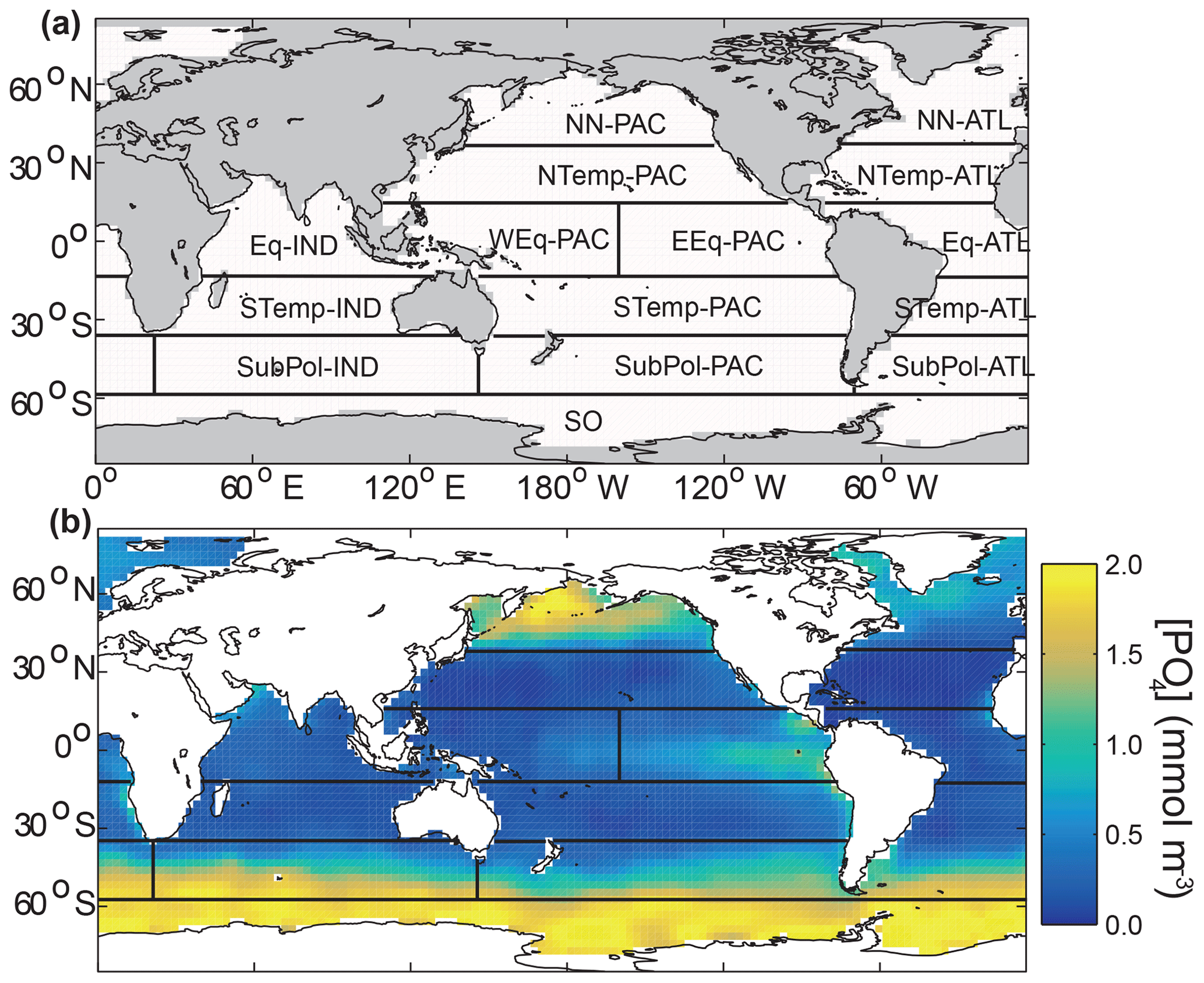
Figure 2(a) Location and names of the 15 regions defined on the model grid based on Gloor et al. (2001). Boundaries are at 58∘ S, 36∘ S, 13∘ S, 13∘ N, and 36∘ N. The equatorial Pacific is split at 98.75∘ E, following Mikaloff Fletcher et al. (2006). Each region can be assigned a value of b that is independent of other regions. (b) Location of regions superimposed on the annual mean surface [PO4] from World Ocean Atlas 2013 (Garcia et al., 2014) regridded to the model grid.
2.3 Experiments
We perform a set of experiments to explore the sensitivity of atmospheric CO2 to regional variability in b with the aim of quantitatively ranking the sensitivity of atmospheric CO2 to remineralization depth changes in each region (e.g. Pianosi et al., 2016):
-
Control run. A pre-industrial control run is set up with export production diagnosed by restoring it to observed surface [PO4] values, a globally uniform Martin exponent of 1.0 and initialized with globally uniform tracer concentrations. Atmospheric CO2 is restored to 278 ppm. A globally uniform Martin exponent gives the lowest volume-weighted root-mean-square misfit compared to annual mean World Ocean Atlas 2013 [PO4] observations (Garcia et al., 2014), as found in other studies using the same MITgcm transport matrices (Kriest et al., 2012). The control run is spun-up from uniform initial conditions for 5000 years.
-
Global sensitivity. The Martin curve is varied globally, i.e. all regions are assigned the same exponent, between 0.4 and 1.6 in 0.1 increments, based on the range of spatial variability observed in the modern ocean (Henson et al., 2012; Marsay et al., 2015; Guidi et al., 2015). Each experiment is run for 3000 years continuing from the control run using the nutrient-restoring scheme to predict export production (Eq. A3) and freely evolving atmospheric CO2.
-
Regional sensitivity. Latin hypercube sampling, a stratified random procedure that provides an efficient way of sampling high dimensional parameter space (McKay et al., 1979), is used to vary the Martin curves in every region simultaneously. Values of b are sampled from a uniform distribution ranging from 0.4 to 1.6 using the “lhsdesign” function in MATLAB with “maximin” sampling (an additional constraint that helps reduce clustering of samples, by maximizing the minimum distance between points, in order to give a well-spread distribution of points across the parameter space). The range of b used centres around b=1.0, as also used for the control run. We generate a Latin hypercube ensemble with 200 experiments, balancing the need for higher sampling resolution of the parameter space and total computational time. Each experiment is run for 3000 years continuing on from the control run with a phosphorus cycle only. Changes in atmospheric CO2 are inferred from changes in preformed PO4.
Both the global and regional sensitivity experiments are repeated with constant-export production that is diagnosed from the control run. All output is diagnosed from the last full simulation year.
2.4 Sensitivity analysis
We use multiple linear regression analysis to derive the sensitivity of atmospheric CO2 to changes in b in each region (k) where the fitted coefficients (βk) give a quantitative measure of the sensitivity (e.g. Pianosi et al., 2016):
3.1 Sensitivity of CO2 to regional variability in remineralization depths
To quantify the sensitivity of CO2 to regional changes in b, we fit linear regression models (Eq. 2) to the results of the Latin hypercube ensembles. The resulting regression models explain a large proportion of the variability between CO2 and b (R2=0.88 and 0.90 for the constant-export and nutrient-restoring ensembles, respectively). Residuals of the regression models showed no significant bias versus the regression output (Fig. S5 in Supplement), suggesting that a linear model was appropriate. Although the relationship between CO2 and a globally uniform remineralization depth is non-linear (e.g. Fig. 6), the relationship is near linear around the observed global mean in the centre of the range of b tested (see also, Kwon et al., 2009). Overall, the absence of a strongly non-linear relationship suggests the use of a linear regression model is appropriate (Pianosi et al., 2016).
When b is varied as a globally uniform parameter from 0.4 to 1.6, atmospheric CO2 varies from 197 to 347 ppm (range of 150 ppm) for the constant-export scheme and from 257 to 288 ppm (range of 31 ppm) for the nutrient-restoring scheme, consistent with previous model experiments (Kwon et al., 2009). Figure 3 shows how the sensitivity of CO2 to changes in b varies as a function of region. CO2 is most sensitive to changes in b occurring in the subantarctic regions, with CO2 being most sensitive to changes in the Indian Ocean sector of the subantarctic (Fig. 3, Table 1). The Southern Ocean and subtropical gyres, with the exception of the gyre in the North Pacific, are consistently the regions where b has the smallest impact on CO2. Other regions, including the equatorial Indian Ocean, equatorial Pacific, and North Pacific have an intermediate sensitivity. As a region, the subantarctic is responsible for ∼30 % of the CO2 sensitivity, comparable to the Pacific basin-scale sensitivity (Table 1).
Table 1Key metrics and sensitivity estimates for each region and basin. Representative metrics including area (percentage of global area), region-integrated mean annual POP export (percentage of global POP export), and mean preformed [PO4] (percentage of global mean) are taken from the control run. CO2 sensitivity estimates for both the nutrient-restoring and constant-export ensembles are given as ΔCO2∕Δb (βk from Eq. 2) with 95 % confidence intervals and as a percentage ().
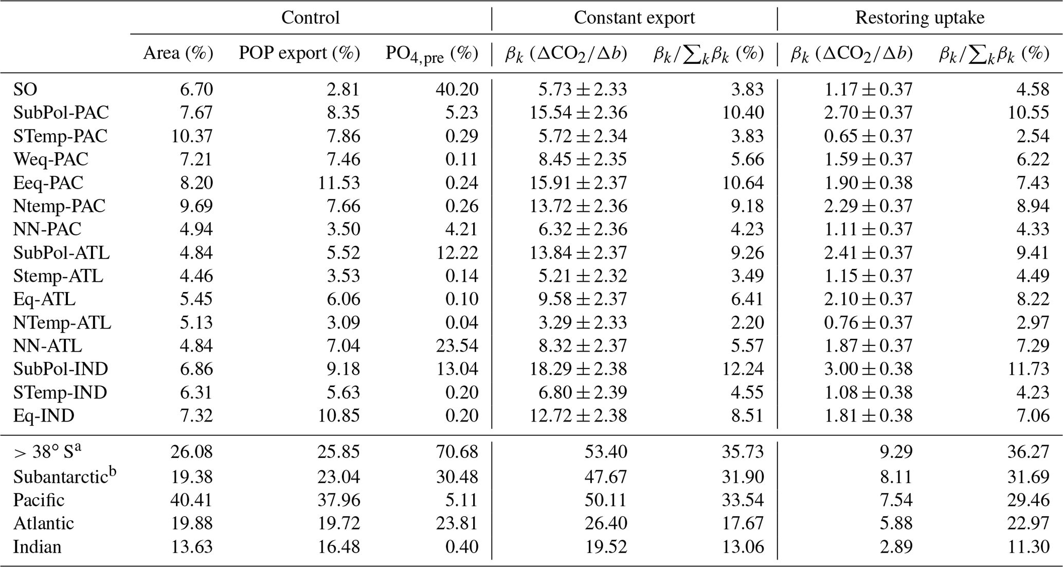
a For comparison with the Southern Ocean estimate, defined as >40∘ S in Kwon et al. (2009). b SubPol-PAC, SubPol-ATL and SubPol-IND.
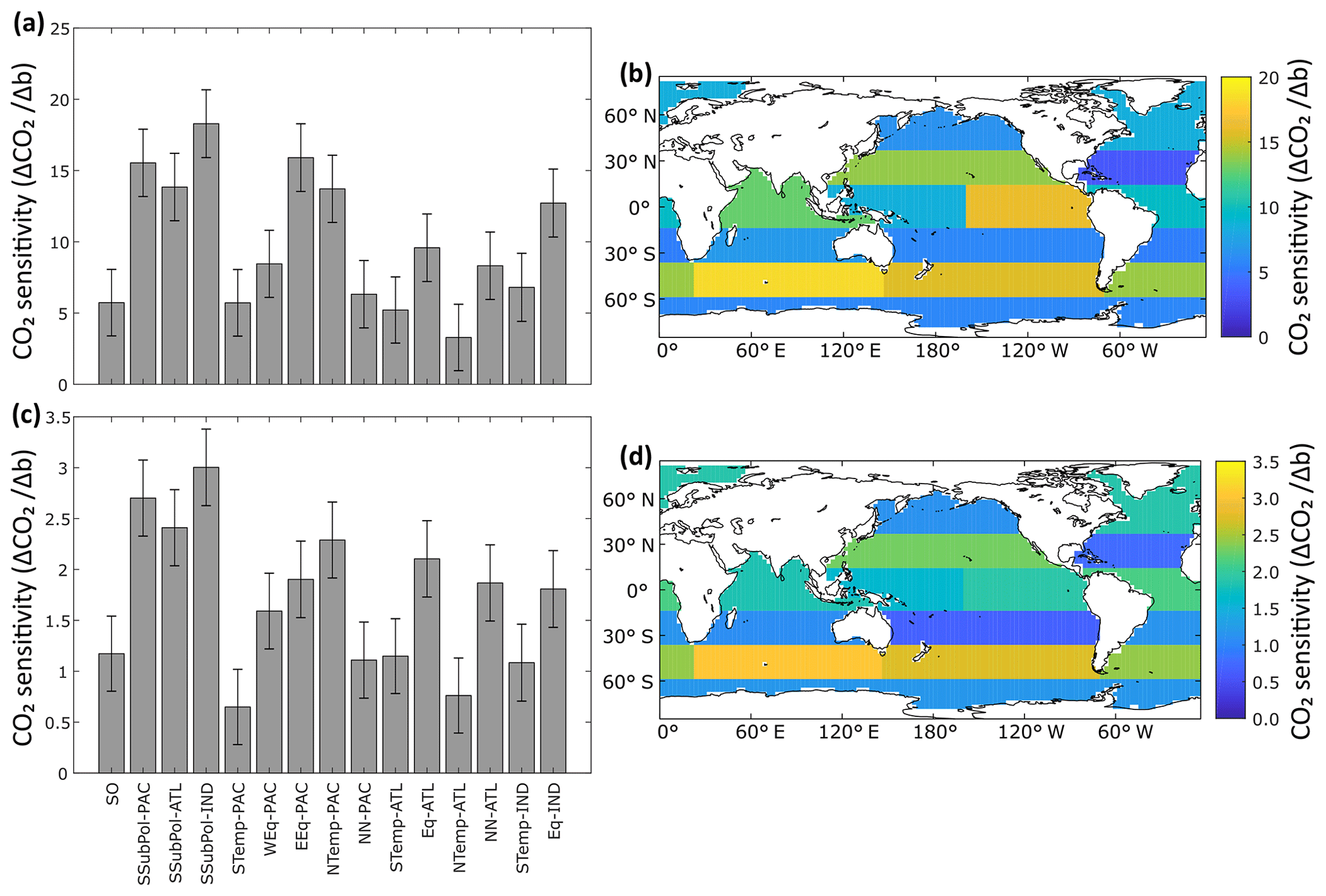
Figure 3Regional sensitivity (ΔCO2∕Δb) of atmospheric CO2 (ppm) to changes in Martin curves for the constant-export scheme (a, b) and nutrient-restoring scheme (c, d). The sensitivity value reflects the increase in CO2 (preformed PO4) for an increase in b (shallower remineralization). Error bars in panels (a) and (c) are 95 % confidence intervals for the linear regression coefficients. Atmospheric CO2 is inferred from modelled preformed PO4 using empirical relationships in Fig. A1 in Appendix A.
As with the globally uniform changes in b, the magnitudes of regional sensitivities are smaller when run using nutrient-restoring uptake as opposed to a constant-export scheme because export production is able to convert any increase in surface nutrient and carbon fluxes back into organic matter, limiting any change in CO2 fluxes. However, the relative sensitivity ranked across regions remains similar, as shown by expressing βk as a percentage of ∑kβk (Table 1). Therefore, the regional patterns in Fig. 3 are not sensitive to assumptions about the response of nutrient uptake to the redistribution of nutrients. This suggests that whilst the absolute magnitude of CO2 sensitivity to changes in b is related to global export production, it is not driven by local changes in export production specific to any region(s).
Kwon et al. (2009) demonstrated that the sensitivity of CO2 to basin-scale changes in b correlated with the magnitude of export production in each basin. Similarly, we find a general positive correlation between sensitivity and regional export production (r=0.79, p<0.01 for constant export; r=0.47, p=0.07 for restoring uptake), as measured by the mean annual average export production across the 200 ensemble runs (Fig. 4). The correlation is much weaker with nutrient-restoring uptake compared to the constant-export production. Intuitively, regions with lower export production, i.e. that contribute less to the inventory of regenerated PO4, have a smaller impact on the balance between preformed and regenerated nutrients and therefore on atmospheric CO2. Whilst CO2 is generally more sensitive to remineralization depths in regions with higher export production, sensitivity varies across regions with similar export production. For example, the sensitivity for the temperate North Pacific (NTemp-PAC; Fig. 4a) (, export production = 1.4±0.11 Tmol P yr−1) is approximately double that of the subpolar region of the South Pacific (STemp-PAC; Fig. 4a) (, export production = 1.4±0.17 Tmol P yr−1). There are no apparent relationships between the variability of export production across the ensemble in each region, as shown by the horizontal error bars, and sensitivity (Fig. 4). This further supports the finding that the response of export production to changes in nutrient distributions are not an important factor in the sensitivity of CO2 to regional changes in b.
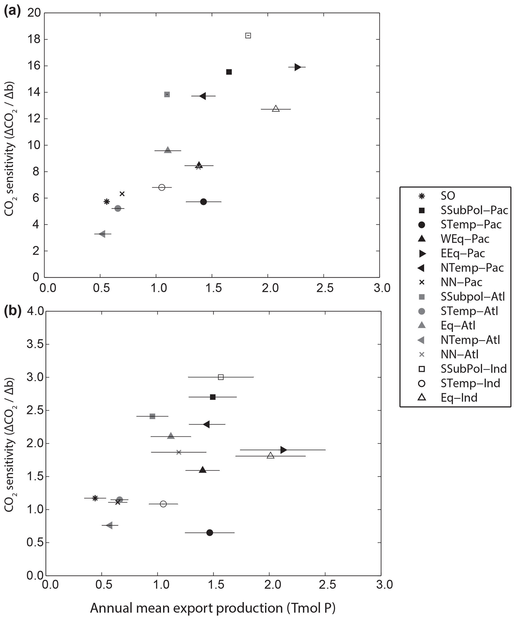
Figure 4Relationship between regional CO2 sensitivity and annual export of PO4 in each region using (a) the constant-export scheme and (b) the nutrient-restoring scheme. Annual export is shown as the mean of the 200 ensemble experiments with ±1 standard deviation error bars.
The variability in sensitivity not explained by the magnitude of POC export is likely a function of how changing remineralization depths interact with ocean circulation. To quantify this effect we calculate the mean preformed PO4 in the ocean interior derived from each region individually (; see Appendix A2.3) and repeat the sensitivity regression analysis. In order to compare regression coefficients from different regions with significantly different magnitudes of we first normalize the concentrations () to the range of variability across the 200 experiments:
The new regression analysis (Eq. 4) now predicts the contribution of changing b in all regions to the change in derived from a single region, rather than globally (Fig. 5). The regression analysis is repeated for each region.
Figure 5 shows the relative sensitivity of to changes in b. R2 ranges from 0.82 to 0.97, suggesting that, overall, the linear regression models are appropriate. The regression coefficients specific to a single region are collected from across the 15 regression results in each column of Fig. 5. By definition, each row of Fig. 5 shows the effect of changing b in the corresponding region on from all other regions.

Figure 5Sensitivity of steady-state normalized mean preformed [PO4] exported from each region (). from each region is expressed as a function of b using linear regression. is normalized to the range of values within each region in the ensemble to account for large differences in preformed between regions. The regression coefficients are arranged such that each row shows the impact of changing b in that region on across other regions. Panels (a) and (b) show the results for the constant-export and nutrient-restoring schemes, respectively.
The sensitivity analysis for each region on an individual basis shows that changes in b in the subantarctic regions have large impacts on across regions globally (Fig. 5). In particular, these regions have a particular effect on the export in the Southern Ocean and in the Atlantic as a basin, comparable in magnitude to the local changes in . Changes in b in the equatorial upwelling regions of the Pacific and Indian Oceans also have a large global effect but with a more pronounced local effect. These features are more pronounced with nutrient-restoring uptake (Fig. 5b). The Southern Ocean and North Atlantic regions are those with the highest export across the ensemble (Table 1), consistent with previous findings about the global importance of these regions for preformed PO4 (DeVries et al., 2012; Pasquier and Holzer, 2016). This suggests the larger sensitivity of CO2 to changes in b in the subantarctic regions is due to the way in which the ocean circulation connects these regions to the Southern Ocean and North Atlantic. In contrast, changing b in the Southern Ocean and North Atlantic has a relatively minimal effect on (and by inference CO2) both locally and globally.
3.2 Regional versus global sensitivity
Lastly, we explore whether the spatial patterns in sensitivity (Fig. 3) are significant on a global scale. Global average values of b are calculated for each of the 200 Latin hypercube samples using an area-weighted mean and compared against experiments where b is perturbed uniformly across regions (Fig. 6). The amount of organic matter reaching the deep ocean is a non-linear function of b, following from the fact that the Martin curve represents the scenario of a fixed remineralization rate and an increasing sinking rate (Kriest and Oschlies, 2008; Cael and Bisson, 2018; see Supplement). Therefore, larger values of b, i.e. shallower remineralization, have disproportionally more weight when calculating a global arithmetic mean of spatially variable b values (Fig. S6). To account for this, we find the equivalent e folding depths for each Latin hypercube sample, which form a skewed distribution due to higher occurrence of shallower remineralization, calculate the area-weighted geometric mean e folding depth for each sample, and re-arrange again for b (see Supplement for details).
The relationship between CO2 and the globally averaged b values from the sensitivity experiments closely matches the relationship between CO2 and globally uniform b for the both constant-export and nutrient-restoring schemes (Fig. 6). Note that b in each region is varied within the full parameter range but because Latin hypercube sampling varies all parameters across their parameter range simultaneously the global mean does not reach the highest and lowest global b values. The average regionally varying b values vary within ppm of the globally uniform experiments with constant-export experiments and ppm for the nutrient-restoring experiments, comparable to the change in CO2 for a globally uniform change in b of ∼0.2.
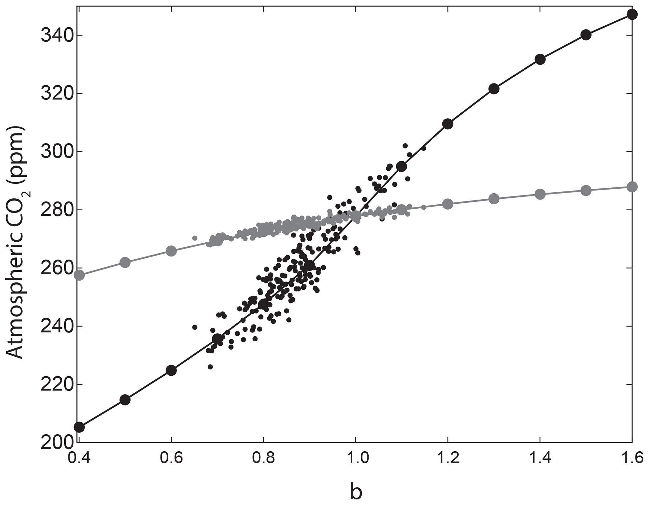
Figure 6Comparison of CO2 sensitivity when b is varied as a globally uniform parameter (solid lines) and when b is varied regionally in the Latin hypercube samples and calculated as an area-weighted geometric mean of e folding depths converted back to b to correct for non-linearities in the Martin curve. Runs using the constant-export scheme are shown in black and nutrient-restoring runs are shown in grey.
Sediment trap observations reveal significant spatial variability in remineralization depths. Here we have quantified the sensitivity of atmospheric CO2 to regional changes in remineralization depths and show that CO2 is most sensitive to changes in the subantarctic regions. Much of the observed spatial variability varies across latitudes (Henson et al., 2012; Guidi et al., 2015; Marsay et al., 2015; Weber et al., 2016). Additionally, the mechanisms potentially driving these patterns are also likely to vary on a latitudinal basis, with changes in related environmental properties in response to anthropogenic CO2 emissions affecting the high latitudes in particular: temperature changes (Kirtman et al., 2013) affecting temperature-dependent remineralization rates, a reduction in carbonate saturation state with ocean acidification (Orr et al., 2005) affecting ballasting and changes in plankton community composition, and cell size (Lefort et al., 2015) affecting aggregation dynamics and particle sinking velocities. Additionally, this is a consideration for changes in remineralization depths occurring in past climates (Meyer et al., 2016). This suggests that the spatial patterns in CO2 sensitivity could be significant when considering the impact of remineralization depth changes.
Changes in the air–sea balance of carbon are commonly related to changes in preformed nutrients. Because of the inefficient utilization of upwelled nutrients in the Southern Ocean, this region has been identified as key to setting the efficiency of the biological pump (Ito and Follows, 2005; DeVries et al., 2012). Our results show that this is also key for the sensitivity of CO2 to regional variability in remineralization depths because of upwelling in subantarctic regions (Fig. 5). This relationship has implications when invoking changes in the efficiency of the biological pump in past climates such as the Last Glacial Maximum (LGM). Processes that increase the utilization of nutrients in the Southern Ocean, such as iron fertilization, and processes that reduce the delivery of nutrients to the Southern Ocean, such as increased stratification, have been implicated in the drawdown of atmospheric CO2 during the LGM (Sigman et al., 2010). Any changes in stratification will also impact the sensitivity of CO2 to any additional changes in remineralization depths, such as from changes in ballasting minerals and/or temperature-dependent remineralization (Chikamoto et al., 2012). In comparison, processes such as iron fertilization will not impact on this sensitivity. Because the spatial patterns of CO2 sensitivity to regional changes in remineralization are predominantly constrained by ocean circulation pathways, this also suggests that the sensitivity may change with a reorganization of ocean circulation as suggested for the LGM (Sigman et al., 2010).
The Martin curve is a commonly used parameterization of the remineralization of particulate organic matter with depth in marine biogeochemical models and is commonly applied with a globally uniform exponent (b) (Hülse et al., 2017). However, the Martin curve used in this way has potential limitations: it is an empirical and static parameterization that does not represent the mechanisms affecting remineralization and sinking rates and it does not capture spatial variability in remineralization observed in sediment trap data (Henson et al., 2012; Marsay et al., 2015; Guidi et al., 2015). In our sensitivity analysis, we have shown that CO2 has a similar sensitivity to the global mean change in b, as compared to a globally uniform change in b with an uncertainty of ±5–15 ppm, equivalent to a change in b of ∼0.2 (Fig. 6). Kwon et al. (2009) suggest a decrease of 0.3 from the modern remineralization depth is sufficient to explain the increase in deep ocean nutrient concentrations during the Last Glacial Maximum. For the 21st century, Laufkötter et al. (2017) predict a decrease in POC export at 500 m by 2100 under RCP8.5 in response to temperature- and oxygen-dependent remineralization, equivalent to a decrease in b of ∼0.25. As such, the global mean change in potential future and past changes in remineralization depth may be larger than the uncertainty associated with spatial variability. This has potentially useful implications for modelling the remineralization of particulate organic matter fluxes. Models resolving the various processes that affect remineralization rates and sinking velocities have recently been developed (Jokulsdottir and Archer, 2016; Cram et al., 2018); however, the requirements to model processes such as particle aggregation can be computationally expensive, limiting their application to 1-D models (Jokulsdottir and Archer, 2016; Cram et al., 2018) or to offline models (DeVries et al., 2014). A globally uniform change in b informed by these models could then be used to calculate the impact on atmospheric CO2 if the change in b is greater than 0.2. However, we note that the modern global mean b is subject to uncertainty associated with under-sampled spatial variability.
Our results are dependent on the use of transport matrices derived from one global circulation model. Whilst this model has been widely applied to study biogeochemistry previously, it is subject to a number of caveats. The ocean model predicts significantly larger outcrops of dense water in the Southern Ocean compared to observations (see Fig. S3 in Supplement, also Duteil et al., 2013), leading to deep-water formation occurring at latitudes around 50∘ S (Fig. S4 in Supplement). The volumetric fraction of water in the ocean interior derived from the subantarctic is also higher (26 %) compared to data-constrained estimates (18 %, Table S1: Khatiwala et al., 2012). As such, the sensitivity estimates for the subantarctic may be overestimated. This is also consistent with the higher sensitivity compared to the basin-scale analysis of Kwon et al. (2009), who found that the Southern Ocean (>40∘ S) contributed 22 % of the global CO2 sensitivity, compared with 36 % in this study (>38∘ S, see Table 1). However, our results have key similarities, including absolute and relative magnitudes of regional preformed PO4 export, to other studies using alternative steady-state circulation states (DeVries et al., 2012; Pasquier and Holzer, 2016). As such, our results should be broadly reproducible with other models. A disadvantage to using a steady-state circulation is that we cannot quantify impact of the CO2–climate feedback on ocean circulation and atmospheric CO2. Studies exploring the simultaneous effects of warming temperatures on circulation and biology in response to anthropogenic CO2 emissions show that changes in circulation could be as important as biological changes (Cao and Zhang, 2017; Yamamoto et al., 2018). Quantifying the regional sensitivity with a dynamic ocean is therefore an important focus for future work. Ratios of CaCO3 to POC vary latitudinally, and could also therefore modify our sensitivity results. Segschneider and Bendtsen (2013) found important feedbacks involving interactions between calcifiers and silicifiers in an marine ecosystem model when exploring temperature-dependent remineralization rates in the 21st century. Future model experiments including a representation of plankton ecosystems would therefore help explore the impact of CaCO3 export on regional sensitivity patterns.
We have presented a sensitivity analysis that quantifies the sensitivity of atmospheric CO2 to regional variability in particulate organic carbon remineralization depths. CO2 is most sensitive to changes in remineralization depths occurring in the subantarctic regions, particularly in the Indian Ocean sector. As a whole, the subantarctic regions have a sensitivity similar to that of the Pacific basin despite the smaller area and levels of production. Sensitivity patterns are in part a function of the magnitude of export production in each region and the physical circulation pathways specific to each region. Whilst the overall magnitude of CO2 sensitivity to regional changes is dependent on the magnitude and response of export production to changes in nutrients, the relative spatial patterns in sensitivity are predominantly constrained by ocean circulation pathways. We also find that the regional variability adds ±5–15 ppm uncertainty to global mean changes in remineralization depths. The regional patterns in sensitivity could be significant if a number of processes that potentially drive changes in remineralization depths, including temperature-dependent remineralization rates and plankton community structure, vary predominantly in the high latitudes. However, this uncertainty is similar to the change in CO2 for a globally uniform change in b of ∼0.2, meaning that larger changes in b could be reliably approximated by a globally uniform b as commonly used in biogeochemical models.
The transport matrices are publicly available at http://kelvin.earth.ox.ac.uk/spk/Research/TMM/TransportMatrixConfigs (Khatiwala, 2019). The model code is freely available at http://github.com/JamieDWilson/Fortran_Matrix_Lab (Wilson, 2019).
The Latin hypercube sampling approach used relies on the ability to run an ensemble of model experiments. To make this approach feasible we use the transport matrix method (Khatiwala et al., 2005; Khatiwala, 2007).
A1 Steady-state ocean circulation model
The matrix used here is the 2.8∘ global configuration of the MIT model with 15 vertical levels driven by seasonally cycling fluxes of momentum, heat, and freshwater (publicly available from http://kelvin.earth.ox.ac.uk/spk/Research/TMM/TransportMatrixConfigs; last access: 29 July 2019). Seasonally varying ocean circulation is calculated at each time step by linearly interpolating between monthly mean matrices. An advantage of using transport matrices is that the time step can be made longer to reduce computational expense (Khatiwala, 2007). Here we extend the circulation time step to 3.8 d.
A2 Biogeochemical model
The biogeochemical model represents the cycle of phosphorus and carbon in the ocean with four dissolved tracers, PO4, dissolved organic phosphorus (DOP), dissolved inorganic carbon (DIC), and total alkalinity. The biogeochemical model has the same time step as the ocean circulation model (3.8 d).
A2.1 Phosphorus cycle
PO4 and DOP are governed by the following equations:
where A denotes the transport matrix calculation of ocean transport and J denotes biogeochemical source and sink terms.
The uptake of PO4 during production of organic matter occurs in the euphotic zone, here defined as the base of the upper two grid boxes (120 m). Following Kwon et al. (2009) we calculate the production of organic matter using either a nutrient-restoring scheme or a constant-export scheme. The nutrient-restoring scheme restores surface concentrations of PO4 to observed [PO4] with a restoring timescale (τ=30 d Najjar et al., 2007) and is scaled by the fraction of sea ice present (Fseaice, as monthly average fields from the original global circulation model):
Organic matter production in the constant-export scheme is fixed to that of the experiment defined as the control run, unless surface [PO4] is depleted below zero, in which case Jup is set to zero at that time step. The control run is defined as having the run with the lowest root-mean-square misfit compared to annual mean World Ocean Atlas [PO4] observations.
A fixed fraction (v=0.66) of the organic matter production integrated across the upper two grid boxes is routed directly to dissolved organic phosphorus (DOP) and remineralized back to PO4 in a first-order reaction with a decay rate of κ throughout the water column:
The remaining fraction of organic matter production () is integrated across the upper two grid boxes and exported as particulate organic phosphorus (POP) at the base of the of the second grid box in the vertical (120 m). The remineralization of POP is parameterized with the Martin curve (Eq. 1). POP that has reached the sediment is remineralized fully in the lowermost grid box of the water column, maintaining a closed system with respect to [PO4]. As such, there is no sediment component in this model.
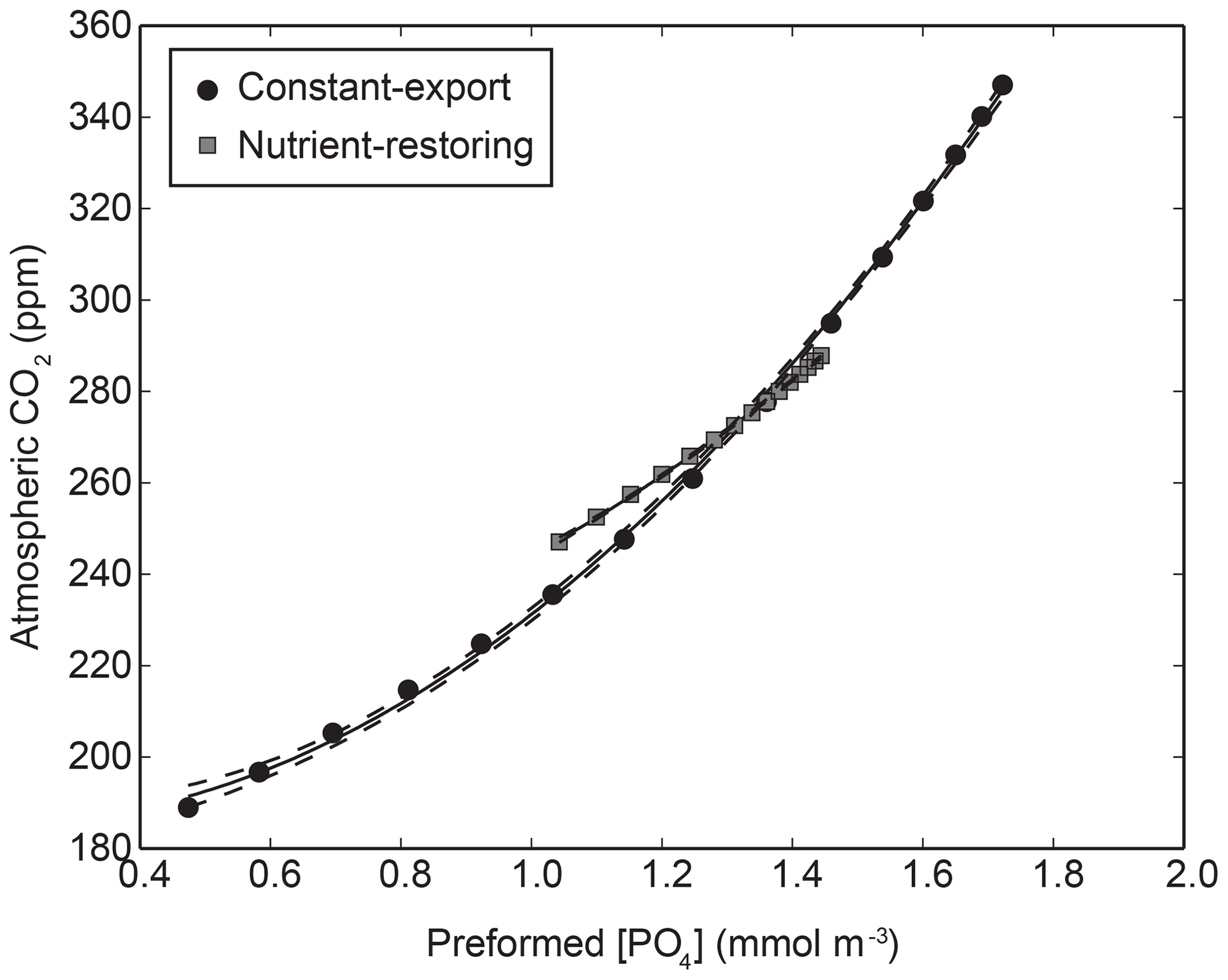
Figure A1Relationship between preformed PO4 and atmospheric CO2 in the biogeochemical model using nutrient-restoring and constant-export schemes when the Martin curve is varied globally between 0.4 and 1.6. A quadratic function () is fitted to the combined data with non-linear least squares is shown with 95 % confidence intervals. The coefficients for the two fits are β1=66.59, and β3=187.09 for constant-export schemes and β1=42.80, and β3=207.95 for nutrient-restoring schemes.
A2.2 Carbon cycle
The uptake of nutrients and remineralization of particulate and dissolved organic phosphorus are related to dissolved inorganic carbon and alkalinity via Redfield ratios of (). Carbonate chemistry parameters are computed from dissolved inorganic carbon and alkalinity using the method described by Follows et al. (2006). The method provides a simplified but accurate solution with computational efficiency. The air–sea gas exchange of CO2 is calculated as per Orr et al. (2017).
A2.3 Preformed PO4 and atmospheric CO2
Changes in atmospheric CO2 due to changes in the biological pump can be directly related to the inventory or average concentration of preformed PO4 (Ppre) if total nutrient concentrations are conserved (Ito and Follows, 2005; Marinov et al., 2008). This provides a way of relating changes in our model of the phosphorous cycle to changes in atmospheric CO2 without simulating a relatively computationally expensive carbon cycle. The distribution of annual mean [Ppre] for each run is calculated by splitting the transport matrices into “interior” matrices (AI) and “exterior” matrices (B) for both the explicit and implicit matrices (subscripts e and i, respectively; see Khatiwala, 2007). The annual mean surface [PO4] from the end of a simulation is set as a boundary condition and solved for the interior distribution of Ppre:
The global mean concentration of Ppre () is related to CO2 using a empirical quadratic function (Eq. A6) fitted to a series of experiments where the Martin curve is varied globally (see below). The function is derived from a non-linear least-squares regression (Fig. A1). The resulting regression fit (details in the caption of Fig. A1) is used to estimate changes in CO2:
The approach to predict CO2 from regional changes in b is evaluated in the Supplement and shows the approach is robust to factors such as the slow timescale for the air–sea gas exchange of CO2 (e.g. Eggleston and Galbraith, 2018).
The supplement related to this article is available online at: https://doi.org/10.5194/bg-16-2923-2019-supplement.
JDW designed the experiments, developed the model code, and ran the model. JDW prepared the manuscript with input from all co-authors.
The authors declare that they have no conflict of interest.
This work is based on research originally conducted as part of a PhD project (Jamie D. Wilson) associated with the UK Ocean Acidification Research Programme (UKOARP). We would like to thank Andrew Yool for his comments on the original research. We also thank Samar Khatiwala for making the transport matrices freely available.
This research has been supported by the Natural Environment Research Council (grant no. NE/H017240/1) and the European Research Council (PALEOGENIE grant no. 617313).
This paper was edited by Carol Robinson and reviewed by four anonymous referees.
Boyd, P. W.: Toward quantifying the response of the oceans' biological pump to climate change, Front. Mar. Sci., 2, 77, https://doi.org/10.3389/fmars.2015.00077, 2015. a
Cael, B. B. and Bisson, K.: Particle Flux Parameterizations: Quantitative and Mechanistic Similarities and Differences, Front. Mar. Sci., 5, 395, https://doi.org/10.3389/fmars.2018.00395, 2018. a
Cao, L. and Zhang, H.: The role of biological rates in the simulated warming effect on oceanic CO2 uptake, J. Geophys. Res.-Biogeo., 122, 1098–1106, https://doi.org/10.1002/2016JG003756, 2017. a
Chikamoto, M. O., Abe-Ouchi, A., Oka, A., and Smith, S. L.: Temperature-induced marine export production during glacial period, Geophys. Res. Lett., 39, L21601, https://doi.org/10.1029/2012GL053828, 2012. a
Cram, J. A., Weber, T., Leung, S. W., McDonnell, A. M. P., Liang, J.-H., and Deutsch, C.: The Role of Particle Size, Ballast, Temperature, and Oxygen in the Sinking Flux to the Deep Sea, Global Biogeochem. Cy., 32, 858–876, https://doi.org/10.1029/2017GB005710, 2018. a, b
DeVries, T., Primeau, F., and Deutsch, C.: The sequestration efficiency of the biological pump, Geophys. Res. Lett., 39, l13601, https://doi.org/10.1029/2012GL051963, 2012. a, b, c
DeVries, T., Liang, J.-H., and Deutsch, C.: A mechanistic particle flux model applied to the oceanic phosphorus cycle, Biogeosciences, 11, 5381–5398, https://doi.org/10.5194/bg-11-5381-2014, 2014. a, b
Duteil, O., Koeve, W., Oschlies, A., Bianchi, D., Galbraith, E., Kriest, I., and Matear, R.: A novel estimate of ocean oxygen utilisation points to a reduced rate of respiration in the ocean interior, Biogeosciences, 10, 7723–7738, https://doi.org/10.5194/bg-10-7723-2013, 2013. a
Eggleston, S. and Galbraith, E. D.: The devil's in the disequilibrium: multi-component analysis of dissolved carbon and oxygen changes under a broad range of forcings in a general circulation model, Biogeosciences, 15, 3761–3777, https://doi.org/10.5194/bg-15-3761-2018, 2018. a
Fay, A. R. and McKinley, G. A.: Global open-ocean biomes: mean and temporal variability, Earth Syst. Sci. Data, 6, 273–284, https://doi.org/10.5194/essd-6-273-2014, 2014. a, b
Follows, M. J., Ito, T., and Dutkiewicz, S.: On the solution of the carbonate chemistry system in ocean biogeochemistry models, Ocean Model., 12, 290–301, https://doi.org/10.1016/j.ocemod.2005.05.004, 2006. a
Garcia, H. E., Locarnini, R. A., Boyer, T. P., Antonov, J. I., Baranova, O. K., Zweng, M. M., Reagan, J. R., and Johnson, D. R.: World Ocean Atlas 2013, Volume 4: Dissolved Inorganic Nutrients (phosphate, nitrate, silicate)., in: NOAA Atlas NESDIS, edited by Levitus, S., U.S. Government Printing Office, Washington, D.C., 2014. a, b, c
Gloor, M., Gruber, N., Hughes, T. M. C., and Sarmiento, J. L.: Estimating net air-sea fluxes from ocean bulk data: Methodology and application to the heat cycle, Global Biogeochem. Cy., 15, 767–782, https://doi.org/10.1029/2000GB001301, 2001. a, b, c
Guidi, L., Legendre, L., Reygondeau, G., Uitz, J., Stemmann, L., and Henson, S. A.: A new look at ocean carbon remineralization for estimating deepwater sequestration, Global Biogeochem. Cy., 29, 1044–1059, https://doi.org/10.1002/2014GB005063, 2015. a, b, c, d, e
Henson, S., Sanders, R., and Madsen, E.: Global patterns in efficiency of particulate organic carbon export and transfer to the deep ocean, Global Biogeochem. Cy., 26, GB1028, https://doi.org/10.1029/2011GB004099, 2012. a, b, c, d, e
Henson, S. A., Sarmiento, J. L., Dunne, J. P., Bopp, L., Lima, I., Doney, S. C., John, J., and Beaulieu, C.: Detection of anthropogenic climate change in satellite records of ocean chlorophyll and productivity, Biogeosciences, 7, 621–640, https://doi.org/10.5194/bg-7-621-2010, 2010. a
Henson, S. A., Sanders, R., Madsen, E., Morris, P. J., Le Moigne, F., and Quartly, G. D.: A reduced estimate of the strength of the ocean's biological carbon pump, Geophys. Res. Lett., 38, L04606, https://doi.org/10.1029/2011GL046735, 2011. a
Hülse, D., Arndt, S., Wilson, J. D., Munhoven, G., and Ridgwell, A.: Understanding the causes and consequences of past marine carbon cycling variability through models, Earth-Sci. Rev., 171, 349–382, https://doi.org/10.1016/j.earscirev.2017.06.004, 2017. a, b
Ito, T. and Follows, M. J.: Preformed phosphate, soft-tissue pump and atmospheric CO2, J. Mar. Res., 64, 813–839, 2005. a, b, c
John, E., Wilson, J., Pearson, P., and Ridgwell, A.: Temperature-dependent remineralization and carbon cycling in the warm Eocene oceans, Palaeogeogr. Palaeocl., 413, 158–166, https://doi.org/10.1016/j.palaeo.2014.05.019, 2014. a
Jokulsdottir, T. and Archer, D.: A stochastic, Lagrangian model of sinking biogenic aggregates in the ocean (SLAMS 1.0): model formulation, validation and sensitivity, Geosci. Model Dev., 9, 1455–1476, https://doi.org/10.5194/gmd-9-1455-2016, 2016. a, b
Khatiwala, S.: A computational framework for simulation of biogeochemical tracers in the ocean, Global Biogeochem. Cy., 21, GB3001, https://doi.org/10.1029/2007GB002923, 2007. a, b, c, d, e
Khatiwala, S.: University of Victoria Earth System Climate Model (ver. 2.9), available at: http://kelvin.earth.ox.ac.uk/spk/Research/TMM/TransportMatrixConfigs, last access: 29 July 2019. a
Khatiwala, S., Visbeck, M., and Cane, M. A.: Accelerated simulation of passive tracers in ocean circulation models, Ocean Model., 9, 51–69, https://doi.org/10.1016/j.ocemod.2004.04.002, 2005. a, b, c
Khatiwala, S., Primeau, F., and Holze, M.: Ventilation of the deep ocean constrained with tracer observations and implications for radiocarbon estimates of ideal mean age, Earth Planet. Sc. Lett., 325–326, 116–125, https://doi.org/10.1016/j.epsl.2012.01.038, 2012. a
Kirtman, B., Power, S., Adedoyin, J., Boer, G., Bojariu, R., Camilloni, I., Doblas-Reyes, F., Fiore, A., Kimoto, M., Meehl, G., Prather, M., Sarr, A., Schar, C., Sutton, R., van Oldenborgh, G., Vecchi, G., and Wang, H.: Near-term Climate Change: Projections and Predictability, in: Climate Change 2013: The Physical Science Basis. Contribution of Working Group I to the Fifth Assessment Report of the Intergovernmental Panel on Climate Change, edited by: Stocker, T., Qin, D., Plattner, G.-K., Tignor, M., Allen, S., Boschung, J., Nauels, A., Xia, Y., Bex, V., and Midgley, P., Cambridge University Press, 2013. a
Kriest, I. and Oschlies, A.: On the treatment of particulate organic matter sinking in large-scale models of marine biogeochemical cycles, Biogeosciences, 5, 55–72, https://doi.org/10.5194/bg-5-55-2008, 2008. a, b
Kriest, I. and Oschlies, A.: MOPS-1.0: towards a model for the regulation of the global oceanic nitrogen budget by marine biogeochemical processes, Geosci. Model Dev., 8, 2929–2957, https://doi.org/10.5194/gmd-8-2929-2015, 2015. a
Kriest, I., Oschlies, A., and Khatiwala, S.: Sensitivity analysis of simple global marine biogeochemical models, Global Biogeochem. Cy., 26, GB2029, https://doi.org/10.1029/2011GB004072, 2012. a, b
Kwon, E. Y., Primeau, F., and Sarmiento, J. L.: The impact of remineralization depth on the air-sea carbon balance, Nat. Geosci., 2, 630–635, https://doi.org/10.1038/ngeo612, 2009. a, b, c, d, e, f, g, h, i, j, k, l, m, n
Lam, P. J., Doney, S. C., and Bishop, J. K. B.: The dynamic ocean biological pump: Insights from a global compilation of particulate organic carbon, CaCO3, and opal concentration profiles from the mesopelagic, Global Biogeochem. Cy., 25, GB3009, https://doi.org/10.1029/2010GB003868, 2011. a
Laufkötter, C., John, J. G., Stock, C. A., and Dunne, J. P.: Temperature and oxygen dependence of the remineralization of organic matter, Global Biogeochem. Cy., 31, 1038–1050, https://doi.org/10.1002/2017GB005643, 2017. a, b
Lefort, S., Aumont, O., Bopp, L., Arsouze, T., Gehlen, M., and Maury, O.: Spatial and body-size dependent response of marine pelagic communities to projected global climate change, Global. Change Biol., 21, 154–164, https://doi.org/10.1111/gcb.12679, 2015. a
Longhurst, A.: Ecological Geography of the Sea, Academic Press, San Diego, 1998. a, b
Marinov, I., Gnanadesikan, A., Sarmiento, J. L., Toggweiler, J. R., Follows, M., and Mignone, B. K.: Impact of oceanic circulation on biological carbon storage in the ocean and atmospheric pCO2, Global Biogeochem. Cy., 22, GB3007, https://doi.org/10.1029/2007GB002958, 2008. a
Marsay, C., Sanders, R., Henson, S., Pabortsava, K., Achterberg, E., and Lampitt, R.: Attenuation of sinking particulate organic carbon flux through the mesopelagic ocean, P. Natl. Acad. Sci. USA, 112, 1089–1094, https://doi.org/10.1073/pnas.1415311112, 2015. a, b, c, d, e
Martin, J., Knauer, G., Karl, D., and Broenkow, W.: VERTEX: carbon cycling in the northeast Pacific, Deep-Sea Res., 43, 267–285, 1987. a, b
McKay, M. D., Beckman, R. J., and Conover, W. J.: A Comparison of Three Methods for Selecting Values of Input Variables in the Analysis of Output From a Computer Code, Technometrics, 21, 239–245, 1979. a
Meyer, K. M., Ridgwell, A., and Payne, J. L.: The influence of the biological pump on ocean chemistry: implications for long-term trends in marine redox chemistry, the global carbon cycle, and marine animal ecosystems, Geobiology, 14, 207–219, https://doi.org/10.1111/gbi.12176, 2016. a, b
Mikaloff Fletcher, S. E., Gruber, N., Jacobson, A. R., Doney, S. C., Dutkiewicz, S., Gerber, M., Follows, M., Joos, F., Lindsay, K., Menemenlis, D., Mouchet, A., Müller, S. A., and Sarmiento, J. L.: Inverse estimates of anthropogenic CO2 uptake, transport, and storage by the ocean, Global Biogeochem. Cy., 20, GB2002, https://doi.org/10.1029/2005GB002530, 2006. a, b
Najjar, R. G., Jin, X., Louanchi, F., Aumont, O., Caldeira, K., Doney, S. C., Dutay, J.-C., Follows, M., Gruber, N., Joos, F., Lindsay, K., Maier-Reimer, E., Matear, R. J., Matsumoto, K., Monfray, P., Mouchet, A., Orr, J. C., Plattner, G.-K., Sarmiento, J. L., Schlitzer, R., Slater, R. D., Weirig, M.-F., Yamanaka, Y., and Yool, A.: Impact of circulation on export production, dissolved organic matter, and dissolved oxygen in the ocean: Results from Phase II of the Ocean Carbon-cycle Model Intercomparison Project (OCMIP-2), Global Biogeochem. Cy., 21, GB3007, https://doi.org/10.1029/2006GB002857, 2007. a
Orr, J. C., Fabry, V. J., Aumont, O., Bopp, L., Doney, S. C., Feely, R. A., Gnanadesikan, A., Gruber, N., Ishida, A., Joos, F., Key, R. M., Lindsay, K., Maier-Reimer, E., Matear, R., Monfray, P., Mouchet, A., Najjar, R. G., Plattner, G.-K., Rodgers, K. B., Sabine, C. L., Sarmiento, J. L., Schlitzer, R., Slater, R. D., Totterdell, I. J., Weirig, M.-F., Yamanaka, Y., and Yool, A.: Anthropogenic ocean acidification over the twenty-first century and its impact on calcifying organisms, Nature, 437, 681–686, https://doi.org/10.1038/nature04095, 2005. a
Orr, J. C., Najjar, R. G., Aumont, O., Bopp, L., Bullister, J. L., Danabasoglu, G., Doney, S. C., Dunne, J. P., Dutay, J.-C., Graven, H., Griffies, S. M., John, J. G., Joos, F., Levin, I., Lindsay, K., Matear, R. J., McKinley, G. A., Mouchet, A., Oschlies, A., Romanou, A., Schlitzer, R., Tagliabue, A., Tanhua, T., and Yool, A.: Biogeochemical protocols and diagnostics for the CMIP6 Ocean Model Intercomparison Project (OMIP), Geosci. Model Dev., 10, 2169–2199, https://doi.org/10.5194/gmd-10-2169-2017, 2017. a
Pasquier, B. and Holzer, M.: The plumbing of the global biological pump: Efficiency control through leaks, pathways, and time scales, J. Geophys. Res.-Oceans, 121, 6367–6388, https://doi.org/10.1002/2016JC011821, 2016. a, b, c
Pianosi, F., Beven, K., Freer, J., Hall, J. W., Rougier, J., Stephenson, D. B., and Wagener, T.: Sensitivity analysis of environmental models: A systematic review with practical workflow, Environ. Modell. Softw., 79, 214–232, https://doi.org/10.1016/j.envsoft.2016.02.008, 2016. a, b, c
Riebesell, U., Kortzinger, A., and Oschlies, A.: Sensitivities of marine carbon fluxes to ocean change, P. Natl. Acad. Sci. USA, 106, 20602–20609, https://doi.org/10.1073/pnas.0813291106, 2009. a
Roth, R., Ritz, S. P., and Joos, F.: Burial-nutrient feedbacks amplify the sensitivity of atmospheric carbon dioxide to changes in organic matter remineralisation, Earth Syst. Dynam., 5, 321–343, https://doi.org/10.5194/esd-5-321-2014, 2014. a
Sarmiento, J. L., Slater, R., Barber, R., Bopp, L., Doney, S. C., Hirst, A. C., Kleypas, J., Matear, R., Mikolajewicz, U., Monfray, P., Soldatov, V., Spall, S. A., and Stouffer, R.: Response of ocean ecosystems to climate warming, Global Biogeochem. Cy., 18, GB3003, https://doi.org/10.1029/2003GB002134, 2004. a
Segschneider, J. and Bendtsen, J.: Temperature-dependent remineralization in a warming ocean increases surface pCO2 through changes in marine ecosystem composition, Global Biogeochem. Cy., 27, 1214–1225, https://doi.org/10.1002/2013GB004684, 2013. a
Sigman, D. M., Hain, M. P., and Haug, G. H.: The polar ocean and glacial cycles in atmospheric CO2 concentration, Nature, 466, 47–55, https://doi.org/10.1038/nature09149, 2010. a, b
Weber, T., Cram, J., Leung, S., DeVries, T., and Deutsch, C.: Deep ocean nutrients imply large latitudinal variation in particle transfer efficiency, P. Natl. Acad. Sci. USA, 113, 8606–611, 2016. a, b, c
Wilson, J. D.: Fortran_Matrix_Lab, available at: http://github.com/JamieDWilson/Fortran_Matrix_Lab, last access: 29 July 2019. a
Yamamoto, A., Abe-Ouchi, A., and Yamanaka, Y.: Long-term response of oceanic carbon uptake to global warming via physical and biological pumps, Biogeosciences, 15, 4163–4180, https://doi.org/10.5194/bg-15-4163-2018, 2018. a