2.1 Site description

The Lena River Delta, one of the largest deltas in the world, is located within the zone of continuous permafrost in northern Siberia (Fig. 1). One of its numerous islands is Samoylov Island (72^∘22^′ N, 126^∘28^′ E), which covers an area of 4.8 km² and features two geomorphological units: the Late Holocene river terrace in the eastern part and the active flood plain in the western part. The carbon dioxide exchange on the river terrace, which is characterised by ice-wedge polygonal tundra with sedges and mosses, has been repeatedly studied (Eckhardt et al., 2019; Kutzbach et al., 2007b; Runkle et al., 2013). In contrast to the river terrace, the flood plain has to date received scarce attention in terms of greenhouse gas fluxes, although active flood plain levels represent roughly 40 % of the soil-covered area of the Lena River Delta (Zubrzycki et al., 2013). Aside from the period of the annual spring flood, whose associated inundation is very variable in magnitude and duration, the flood plain on Samoylov Island stretches over an area between 1 km² (spring) and 2 km² (autumn). More importantly, the surface of the flood plain exhibits, in opposition to the river terrace, a distinct heterogeneity on the mesoscale.

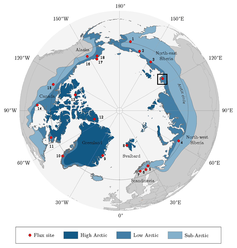
Figure 1Location of the Lena River Delta in northern Siberia indicated by the square. The dots point out sites that were utilised for the pan-Arctic comparison of carbon dioxide budgets (Table 3). The classification of the Arctic zones was based on vegetation occurrence (modified from AMAP, 1998). Accordingly, the treeline delimits the (terrestrial) Arctic; i.e. it corresponds with the boundary between sub-Arctic and low Arctic.

Download

The central delta region is situated in a continental Arctic climate, which is characterised by very low temperatures and a low annual precipitation. In the distant town of Tiksi, located around 120 km southeast of Samoylov Island, a mean annual air temperature of −12.8 ^∘C was measured during 1936–2016 and a mean annual precipitation of 329 mm was gauged during 1956–2016 (AARI, 2017). Additional information on this study site can be found in Rößger et al. (2019a).

2.2 Experimental setup and data recording

An eddy covariance system was installed in the southern part of the flood plain, and the measurements covered two periods: 18 June to 2 October 2014 (107 d) and 9 June to 24 September 2015 (108 d).

The flux tower was equipped with a sonic anemometer (CSAT3, Campbell Scientific, UK) and a gas analyser for water vapour and carbon dioxide (LI-7500A, LI-COR Biosciences, USA). Both instruments were mounted at a height of 2.83 m and sampled with a frequency of 20 Hz. In addition, another eddy covariance system with the same instrumentation has already been deployed at a central position on the adjacent river terrace (Holl et al., 2019).

Supplementary measurements on the flood plain involved gathering data of both air temperature (HMP45, Campbell Scientific, UK) and photosynthetic photon flux density (SKP215, Skye Instruments, UK). These environmental variables were recorded on a logger (CR1000, Campbell Scientific, UK) in quarter-hourly intervals. Furthermore, a time-lapse camera (TLC200, Brinno, Taiwan) was mounted on the flux tower, pointing northeast, for monitoring the phenology during spring 2014 with the same interval of a quarter of an hour.

An acquisition of data on the footprint's surface structure was intended by employing ground-based LAI measurements, as this quantity is widely applied for characterising plant canopies. However, on account of the low height of lichens, mosses and sedges, the measurements with an upwards-pointing sensor (LAI-2200C, LI-COR Biosciences, USA) yielded poor quality results. Therefore, the measurements were terminated after a few test surveys.

2.3 Flux processing

The flux computation was carried out with the software EddyPro version 6.0.0 (LI-COR Biosciences, 2016) for 30 min flux intervals and followed the standard procedure. Detailed information on the executed (i) raw data processing (spike removal, coordinate rotation, block averaging, time lag compensation), the implemented (ii) flux correction scheme (density correction, spectral correction in low- and high-frequency ranges, flux error estimation), and the conducted (iii) quality assessment routine (stationarity test, integral turbulence characteristics test, skewness and kurtosis examination, energy flux quality verification, signal strength control, percentile removal) is provided in Rößger et al. (2019a).

For the footprint modelling, an analytical model for non-neutral stratification was employed (Kormann and Meixner, 2001). This model is based on a stationary gradient diffusion formulation with height-independent crosswind dispersion (Leclerc and Foken, 2014). When applying the solution of the resulting two-dimensional advection–diffusion equation for solving the power law profiles of both eddy diffusivity and mean wind velocity, it yielded a source weight function for each flux interval.

2.4 Surface structure

For studying the impact of the heterogeneous surface on the flux variability, the entire flood plain was mapped in August 2014 by employing helicopter-based visible aerial imagery. The resulting geo-referenced orthomosaic exhibited a resolution of 8.5 cm and hence provided very detailed spatial information, which was sufficient to resolve the pronounced heterogeneity of the surface. Based on maximum likelihood classification tools, the vegetation was classified employing a supervised classification routine on the orthomosaic (Fig. 2). In this process, four different land cover classes were utilised, two of which represent the vegetation.

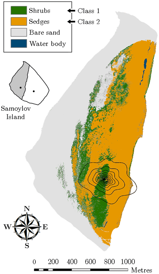
Figure 2Vegetation map of the flood plain on Samoylov Island obtained through supervised classification of a high-resolution orthomosaic. The flux tower was situated in the centre of the footprint isolines, which indicate the averaged area from which 10 %–90 % (increments of 10 %) of the flux originated during the measurement periods of 2014 and 2015 (footprint climatology). The small inset illustrates Samoylov Island being composed of flood plain (grey) and river terrace (white) plus the location of their respective flux towers.

Download

Vegetation class 1 (“shrubs”) refers to sites, which were densely vegetated by large dwarf shrubs of the willow family such as Salix pulchra, Salix lanata, Salix hastata, Salix glauca, growing to a maximum height of around 1 m. This shrubby vegetation was located on a sandy ridge aligned in the north–south axis. The elevated area enabled, in conjunction with a spatially averaged maximum thaw depth of 0.93 m, a good drainage. Since the groundwater table remained at depths around 50 cm, the surface was mostly dry, forming favourable growing conditions for willow shrubs and a sparse cover of thin moss.

Vegetation class 2 (“sedges”) represents areas, which were dominated by sedges including Carex aquatilis, Carex chordorrhiza, Carex concolor, as well as species of Eriophorum and Equisetum. Also, small willow shrubs growing to a height of about 0.3 m were occasionally to be found. This predominantly graminoid vegetation was located in depressions around the dry ridge and exhibited a mean active layer depth of 0.69 m. Accordingly, the soil moisture conditions alternated between moist surfaces and wet patches with water levels up to 40 cm. The ample moisture attracted many mosses forming a dense cover of thick moss.

The two other classes, which do not occur in the 90 % contribution footprint around the flux tower, denote a large area of bare sand along the waterfront and some small water bodies mainly situated in the northern part of the flood plain (Fig. 2). The former class was not considered in the budget estimation since its carbon dioxide flux rates were (in comparison to the two vegetation classes) assumed negligible. The latter class was appended to vegetation class 2 as the few small water bodies surrounded by sedges were presumed to have similar flux rates. Further information on the classification routine is given in Rößger et al. (2019a).

2.5 Flux modelling

The model structure was based on the computation of the two components of the carbon dioxide flux.

$F_{{\mathrm{CO}}_{\mathrm{2}}}$ is the net carbon dioxide flux observed at the flux tower and is equal to the net ecosystem exchange (NEE). Its two components describe, respectively, the total ecosystem respiration (TER) and the gross primary productivity (GPP), both of which can be modelled simultaneously (Runkle et al., 2013).

R_base denotes the basal respiration at the reference temperature (T_ref), which was set to 15 ^∘C, and a scaling factor (γ) was held constant at 10 ^∘C (Mahecha et al., 2010). Q₁₀ indicates the temperature sensitivity; i.e. this parameter is a value by which respiration multiplies/divides, when the temperature rises/drops by 10 ^∘C. P_max refers to the maximum photosynthetic potential and quantifies the theoretical maximum of photosynthesis at infinite irradiance. α represents the light sensitivity and states, as the initial quantum efficiency, the slope of the light response curve at irradiance of zero. All of the four (physiologically interpretable) parameters are best-fit parameters, which were estimated via non-linear ordinary least-squares regression utilising both air temperature (T_air) and photosynthetic photon flux density (PPFD) as explanatory variables. In order to take the heterogeneous surface structure into account, footprint information was included, forming the final model employed for carbon dioxide flux modelling.

Another explanatory variable is the relative contribution of each vegetation class to the flux (Ω) that weights the two computed vegetation-specific fluxes. This variable was obtained through (i) computing the source weight function for a flux interval, (ii) spatially discretising this continuous function with a resolution of 1 m, (iii) adjusting the vegetation map to a resolution of 1 m, (iv) assigning each value of the source weight function to its spatially corresponding vegetation class, and (v) summing the values in each vegetation class.

The fitting procedure, in which only half-hourly quality-controlled flux data were employed, required the estimation of a large number of fitting parameters: R_base, Q₁₀, P_max, α for each vegetation class (Fig. 3). In order to avoid overparameterisation and equifinality problems, the model structure was gradually simplified along four different steps. These alterations in the parameterisation enabled the desired estimation of (i) reasonable seasonal courses of the fitting parameters, i.e. courses that displayed a predominantly smooth evolution with elevated values during the growing season and low values in the shoulder seasons, and (ii) meaningful and significant values for the fitting parameters, i.e. values that were within an acceptable range and their 95 % confidence interval did not overlap zero. Achieving both objectives provided the possibility to interpret the fitting parameters ecophysiologically.

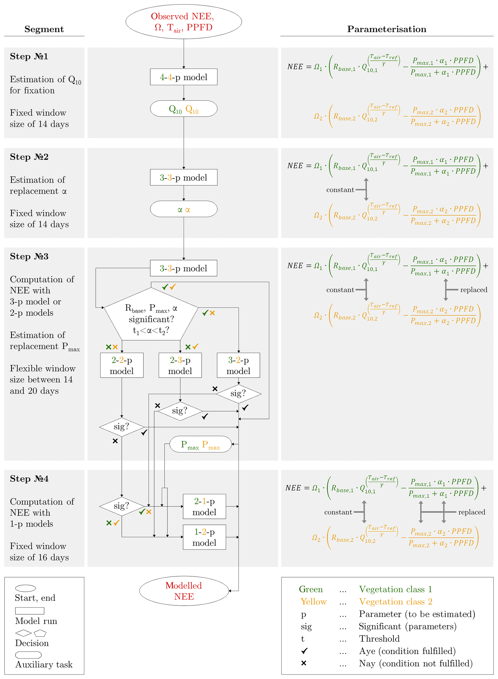
Figure 3Schematic overview of the model calibration along four steps, in which different parameterisations were applied to obtain meaningful estimates for the eight fitting parameters (R_base, Q₁₀, P_max, α for each vegetation class). The values in the boxes (e.g. 3-2-p model) denote the number of parameters to be fitted for each vegetation class.

Download

In each of the four parameterisation steps, the respectively parameterised model was recalibrated for every day, applying a moving window with fixed/flexible window sizes and a step size of 1 d. In the initial step (step 1), which served the computation of representative Q₁₀ values, all of the eight fitting parameters were estimated in the model (4-4-p). Through its output, which encompassed eight best-fit time series, a representative Q₁₀ value was obtained for each vegetation class by determining the median out of the best-fit Q₁₀ values that fulfilled two requirements: statistical significance and an associated coefficient of determination (between observed NEE and modelled NEE) of 0.75 or greater. These two Q₁₀ values were held constant in the further fitting procedure. In the subsequent step (step 2), the simplified model (3-3-p) was run with six fitting parameters to be estimated, and a Gaussian bell curve was fitted to the time series of significant best-fit α values for each vegetation class. By adding/subtracting 30 % of the function values to/from these two replacement functions, a pair of encompassing threshold functions was respectively appended. These intervals around the replacement functions formed a range inside which best-fit α values were accepted. In the following step (step 3), the model (3-3-p) was run with the same parameterisation of the previous step. The model output was checked for α values inside the acceptable interval as well as significant values for R_base, P_max and α. If these criteria were satisfied, the accordingly modelled NEE was approved, and the fitting procedure proceeded to the next day. Alternatively, several models (3-2-p/2-3-p/2-2-p) were run employing α value(s) from the replacement function(s) for one or both vegetation classes, depending on which vegetation class insignificant and/or implausible best-fit parameters were in. The output was tested again, and in case of significant best-fit parameters, the modelled NEE was accepted, and the fitting procedure continued with the next day. Lastly, a replacement function for P_max was created by fitting a Gaussian bell curve to the time series of significant best-fit P_max values in both vegetation classes. In the final step (step 4), two greatly simplified models (2-1-p/1-2-p) were run with only three fitting parameters to be estimated, as well as a P_max value from the replacement function. Here, if not before, all fitting parameters have taken on meaningful and significant values, which ensured the computation of reliable NEE values. In addition to this brief explanation, a detailed description of the entire fitting process is attached in the Appendix.

Since the model was designed to simultaneously compute the component fluxes in both vegetation classes, it provided the capability for the decomposition of the observed fluxes into their separate flux contributions by the two vegetation classes. The reliability of this downscaling, however, was dependent on the restrictive acceptance of meaningful and significant values for the fitting parameters. The temporal integration of these partitioned fluxes and the subsequent projection of the resulting budgets on their corresponding areas on the flood plain formed the upscaling. The summation of both vegetation class budgets finally yielded a robust budget of the entire flood plain, which was designated as the area of interest. This budget, as opposed to the directly estimated footprint budget, did not exhibit a sensor location bias and hence allowed an unbiased appraisal of both the interannual variability and the sink/source strength. For the sake of comparability of the budgets between the years, the carbon dioxide budgets were calculated for the comparison period of 18 June to 24 September, where data were available in both years. The utilised methane budgets, being necessary for estimating greenhouse gas sink/source strengths, have been obtained for the same period and in a similar fashion to the carbon dioxide fluxes, i.e. an initial downscaling of the observed net fluxes and a subsequent upscaling of the decomposed fluxes on the flood plain (Rößger et al., 2019a).

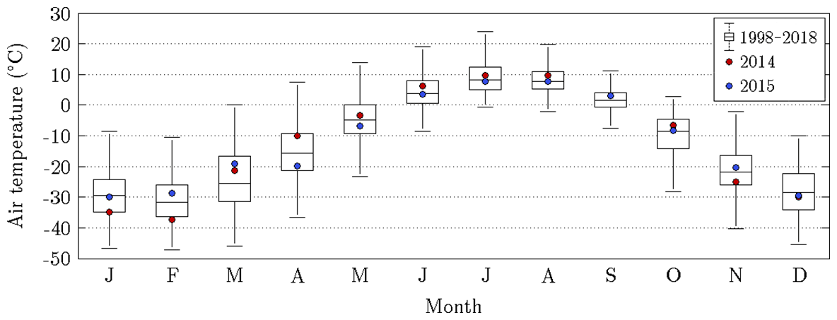
Figure 4Annual course of air temperature on Samoylov Island for the years 2014 and 2015, as well as the recent 20-year baseline (Boike et al., 2013, 2019). In each box plot, the central mark denotes the monthly median, and the bottom and top edges indicate the 25th and 75th percentiles, respectively. The whiskers extend to the most extreme data points excluding outliers. During the warm season, when flux data were available (June to September), 2014 was mostly warmer than 2015.

Download

3.1 Meteorological conditions

The mean air temperatures during the measurement periods in 2014 and 2015 amounted to 7.7 and 7.1 ^∘C, respectively. Furthermore, the respective precipitation sums totalled 92.3 and 130.4 mm. The assessment of these values was based on their comparison with long-term averages that were obtained for Samoylov Island between 1998 and 2018 (Fig. 4). The measurement period in 2014 was on average distinctively warmer and slightly drier, while the measurement period in 2015 featured the same mean temperature as the baseline but considerably more rain. The largest differences in air temperature between both measurement periods occurred in spring. Accordingly, the snowmelt in 2014 took place in a prolonged manner during mid-May already, whereas in 2015, the snowmelt was completed within a couple of days in early June, as usual.

3.2 Dynamics of observed fluxes

The carbon dioxide fluxes exhibited both a diurnal and a seasonal course with the following mean fluxes that were obtained by averaging half-hourly flux data for the subseasons in both 2014 and 2015 (Fig. 5). Between the snowmelt and the vegetative phase, the mean carbon dioxide fluxes remained slightly positive, indicating a prevalent respiration, while the vegetation largely remained dormant (0.26 µmol m⁻² s⁻¹). With the onset of the growing season in late June, stalks and foliage began to develop, and the uptake of carbon dioxide during daytime outweighed the release of carbon dioxide during nighttime (−1.06 µmol m⁻² s⁻¹). The intensity of this oscillation increased towards the onset of the reproduction phase in mid-July, where flowers and seeds developed. During this phase, the most negative fluxes occurred featuring a relatively constant magnitude (−1.77 µmol m⁻² s⁻¹). With the onset of the ripening phase in early August, bushes and sedges attained full maturity, and the flux amplitude of the diurnal cycle began to be progressively attenuated (−0.78 µmol m⁻² s⁻¹). During the nights of this period, the most positive fluxes occurred. Towards late August, the respiration exceeded photosynthesis again, indicating the onset of the senescence phase, which was associated with both leaf colouration and leaf drop (0.39 µmol m⁻² s⁻¹). After the end of the growing season in early September, when abscission was completed, the dominance of respiration continued to grow, leading to more positive mean carbon dioxide fluxes (0.55 µmol m⁻² s⁻¹).

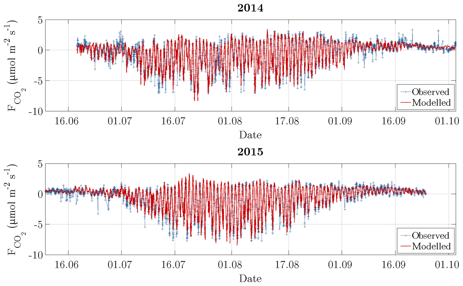
Figure 5Time series of observed carbon dioxide fluxes (after conducting the quality assessment) and modelled fluxes. During the growing season, which is indicated by an elevated variability between late June and early September, the daytime uptake directly followed the diurnal cycle of PPFD, while the nighttime release was dependent on air temperature.

Download

3.3 Model calibration and performance

While the Q₁₀ values were optimised at constant values of 1.42 for vegetation class 1 and 1.48 for vegetation class 2, the other fitting parameters (R_base, P_max and α) displayed a seasonal course for each vegetation class in 2014 and 2015 (Figs. 6 and 7). The temporal evolution of α values could be well approximated with replacement functions, whose application reduced the noise not only in the seasonal courses of α but also in the seasonal courses of both R_base and P_max. In contrast to the replacement functions of α, which were created for both vegetation classes in both years, a replacement function for P_max was created only for vegetation class 1 in 2015 and for vegetation class 2 in 2014.

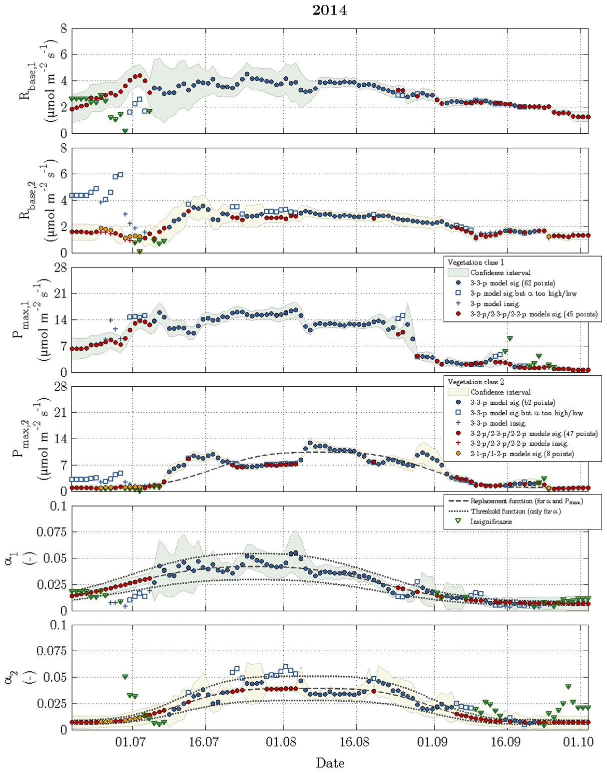
Figure 6Time series of fitting parameters in 2014 for vegetation class 1 (index 1 and green confidence intervals) and vegetation class 2 (index 2 and yellow confidence intervals). The circles represent acceptable fits, while the respective reasons for reparameterisation such as insignificant values or values out of valid range are indicated by plus signs and squares. The triangles denote the fitting parameter(s), which caused a refit in the corresponding vegetation class.

Download

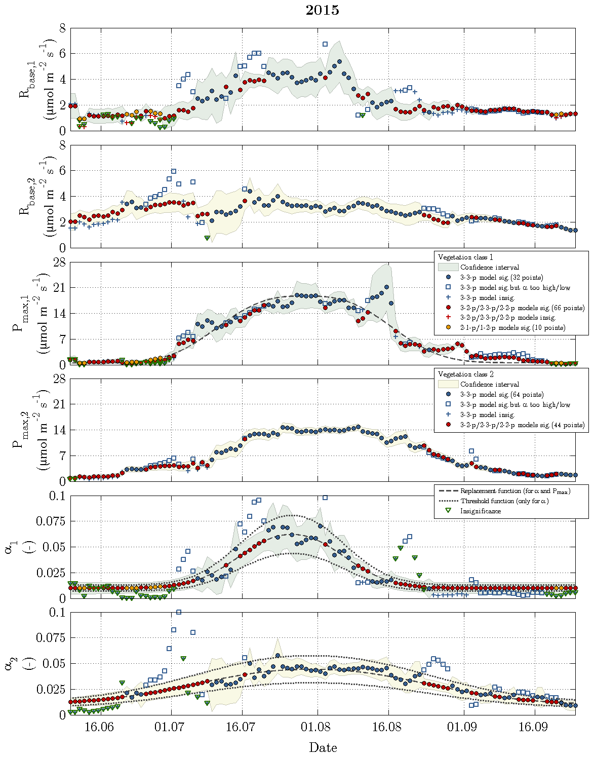
Figure 7Time series of fitting parameters in 2015 with the same symbols and colours as utilised in the previous figure.

Download

The slightly simplified 3-3-p model, which was run at the start of step 3, yielded meaningful and significant values for the fitting parameters in 49 % of the modelled days including 2014 and 2015 (Fig. 3). In the further course of step 3, these goals were achieved by the gradually simplified 3-2-p/2-3-p/2-2-p models in 47 % of the modelled days. During the remaining 4 %, the greatly simplified 2-1-p/1-2-p models of step 4 were deployed. While the 3-3-p model was mainly employed during the summer season, the 3-2-p/2-3-p/2-2-p models were applied throughout the measurement periods with a focus on the shoulder seasons. The 2-1-p/1-2-p models were solely deployed during the shoulder seasons and more often during spring than during autumn. Hence, larger fluxes during the growing season could be more easily modelled in comparison to the remaining time, when lower fluxes associated with a less favourable signal-to-noise ratio prevailed.

R_base was the fitting parameter that could be estimated most confidently, as this parameter accounted for only 19 % of the insignificant values obtained during the fitting procedure in 2014 and 2015. While P_max caused 31 % of the insignificance values, α appeared to be the least certain fitting parameter representing the remaining 50 %. Furthermore, P_max featured most of the significant differences in best-fit values between both vegetation classes, i.e. the confidence intervals of vegetation classes 1 and 2 rarely overlapped, whereas best-fit α values exhibited the fewest significant differences.

On account of both the recalibration for each day as well as the coinciding variabilities of explanatory variables and the explained variable, the model was able to reproduce the observed fluxes very well (Fig. 5). This performance was expressed by a coefficient of determination (R²) of 0.88 for 2014 and 0.95 for 2015. Furthermore, the mean absolute error (MAE) amounted to 0.49 and 0.35 µmol m⁻² s⁻¹ for 2014 and 2015, respectively, while the root mean square error (RMSE) amounted to 0.75 and 0.52 µmol m⁻² s⁻¹. During the summer season, the model performed better in comparison to the shoulder seasons, where autumn in turn displayed a slightly better performance than spring.

3.4 Downscaling and upscaling of fluxes

The estimation of vegetation-class-specific parameter sets allowed the decomposition of the observed net fluxes. This downscaling yielded fluxes of NEE plus their component fluxes (TER and GPP) accounting for both vegetation classes in both years (Fig. 8). For the comparison period in 2014, the mean NEE amounted to −0.89 and −0.38 µmol m⁻² s⁻¹ for vegetation class 1 and vegetation class 2, respectively, and for the comparison period in 2015, −0.71 and −0.69 µmol m⁻² s⁻¹ (Table 1). In contrast to the similar mean net uptakes in 2015, the mean net uptakes in 2014 distinctly differed from each other. This discrepancy originated from the first half of the growing season (mid-June to early August), when the net uptake of vegetation class 1 was considerably larger relative to vegetation class 2. During the second half of the growing season (early August to late September), both net uptakes were rather similar again. Furthermore, the differences in the net uptakes between both years were governed by changes in GPP rather than in TER. In vegetation class 1, NEE in 2014 was only slightly greater in comparison to 2015, which can be attributed to a greater TER and a distinctly greater GPP. And in vegetation class 2, NEE in 2014 was smaller compared to 2015, which can be ascribed to a smaller TER and a clearly smaller GPP.

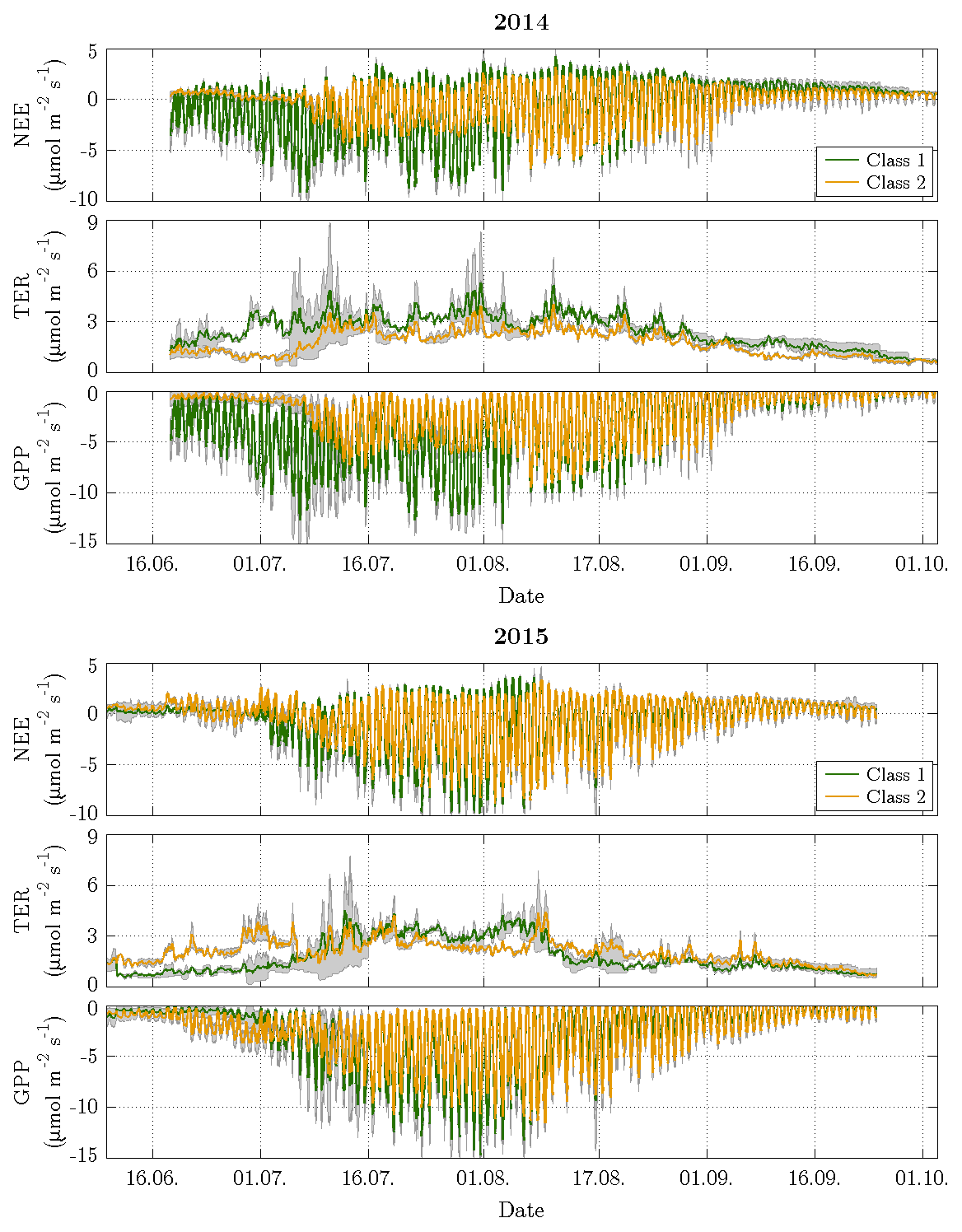
Figure 8Time series of decomposed fluxes with 95 % confidence intervals for both vegetation classes. The width of the confidence intervals varied depending on both the flux magnitude and the number of fitting parameters in the chosen model. The decomposition revealed a distinct difference in the net uptake between both vegetation classes during the first half of the growing season in 2014, while the flux dynamics of both vegetation classes were rather similar during the remaining time and in 2015.

Download

Table 1Outcome of downscaling and upscaling carbon dioxide fluxes for the comparison period (18 June to 24 September) in both 2014 and 2015. The mean downscaled fluxes (± standard deviation) refer to the individual fluxes of both vegetation classes (Fig. 8). Their aggregation yielded cumulative fluxes, whose projection on their corresponding areas on the flood plain in turn returned upscaled fluxes (± combination of cumulative flux error and classification error). The uncertainty metrics derived from the comparison of the applied vegetation map, which was obtained through supervised classification of aerial imagery, with another vegetation map that was acquired via ground-based surveys (Rößger et al., 2019a).

Download Print Version | Download XLSX

The aggregation of the decomposed fluxes over the comparison period yielded individual budgets, whose multiplication with the corresponding fractional coverages on the flood plain formed the upscaling (Table 1). The subsequent summation of both vegetation-class-specific net uptakes returned the net uptake of the entire flood plain for the comparison period: $-\mathrm{4.42}\pm \mathrm{0.49}$ Mmol in 2014 and $-\mathrm{6.17}\pm \mathrm{0.66}$ Mmol in 2015. The stated uncertainties were obtained by means of standard error propagation techniques including both cumulative flux error and classification error, where the former was an order of magnitude smaller than the latter. Dividing these budgets by the total area of the flood plain yielded mean flood plain budgets of $-\mathrm{4.22}\pm \mathrm{0.47}$ and $-\mathrm{5.89}\pm \mathrm{0.63}$ mol m⁻² (Table 2). These budgets consider the surface heterogeneity; i.e. they are corrected for the sensor location bias, plus they contain an areal reference and thus enable an appropriate comparison with other sites.

Table 2Comparison of the sink/source strengths between flood plain and river terrace for the comparison periods in 2014 and 2015 (Holl et al., 2019; Rößger et al., 2019a). Accounting for methane's radiative efficiency as a potent greenhouse gas, the methane budgets were converted to carbon dioxide equivalents with a factor of 34, which corresponds to methane's global warming potential based on a time horizon of 100 years including climate carbon feedbacks (Myhre et al., 2013). The flood plain budgets are given for each vegetation class and for the total area. These budgets are the result of a scaling procedure, which included fairly large classification errors that caused distinctly greater uncertainties in comparison to the river terrace budgets, which derived from a representative footprint and hence did not undergo any scaling processes. In comparison to the flood plain, the polygonal tundra on the river terrace took up less carbon dioxide per square metre, but also released less methane, resulting in a similar (2014) and weaker (2015) sink strength for greenhouse gases.

Download Print Version | Download XLSX

3.5 Greenhouse gas balances

The evaluation of the flood plain's sink/source strength for greenhouse gases required the corresponding methane emission budgets and their conversion to carbon dioxide equivalents (Rößger et al., 2019a). Despite methane's minor percentage of roughly 3 % in the entire greenhouse gas exchange (specified in molar units), its carbon dioxide equivalents diminished the greenhouse gas sink strength (given by the carbon dioxide net uptake) by half in 2014 and by one-third in 2015. Accordingly, the greenhouse gas balances specify that the flood plain formed a moderate sink of $-\mathrm{2.21}\pm \mathrm{0.61}$ mol CO₂ eq. m⁻² and a stronger sink of $-\mathrm{3.81}\pm \mathrm{0.74}$ mol CO₂ eq. m⁻² during the warm season in 2014 and 2015, respectively (Table 2). The lower sink strength in 2014 was a result of a reduced carbon dioxide net uptake rather than an augmented methane efflux. And this reduced carbon dioxide net uptake in turn was caused by a lowered net uptake in vegetation class 2 that effectively counteracted the elevated early season net uptake in vegetation class 1. This class constituted a stronger greenhouse gas sink than vegetation class 2 in both years, which is mainly due to the fact that methane emissions were only present in vegetation class 2. Since these emissions hardly changed between the years along with the negligible methane release in vegetation class 1, the interannual variability in the greenhouse gas sink strength was governed by the carbon dioxide net uptake.

These balances are the first greenhouse gas budgets of a flood plain in the Lena River Delta. Based on these budgets, the sink strength of the adjacent river terrace, where another eddy covariance system has been in operation for many years, could finally be put in context within the domain of the Lena River Delta (Table 2). In 2014 and 2015, the flood plain sequestered per square metre roughly 20 % and 60 % more carbon dioxide, respectively, but it also emitted approximately 70 % more methane. Hence, the flood plain constituted a sink for greenhouse gases that resembled (2014) or was 1.5 times (2015) the sink strength of the polygonal tundra on the river terrace.

4.1 Assessment of the flux decomposition model

The partitioning of carbon dioxide fluxes was conducted during the Arctic summer, when fully dark conditions during the nights were absent. Consequently, a partitioning approach that is based on fitting parameters to nighttime respiration followed by extrapolating these fits to daytime, and subsequently subtracting the estimated daytime respiration flux from the observed net flux to obtain the photosynthesis flux is confronted with elevated uncertainties (Reichstein et al., 2005). The partitioning approach of the present study avoids this problem since the parameter fitting employs the entire data set. However, the model may have a shortcoming in the small number of environmental driving parameters, which may oversimplify the complex biogeochemical processes involved in the carbon dioxide exchange between soils, plants and the atmosphere. While the entire temperature sensitivity of the modelled NEE is manifested through changes in TER, the effect of temperature on the biochemical reactions in GPP is neglected (Haraguchi and Yamada, 2011). At the same time, no correlation between air temperature and model residuals could be detected (homoscedasticity), which indicates that the temperature-induced variability was sufficiently considered. The confounding effect of a high vapour pressure deficit (VPD), which tends to take place in the afternoon, leading to a limited photosynthetic activity, was not taken into account (Lasslop et al., 2010). However, only very few days with low humidity (VPD >10 hPa) occurred, and the typically asymmetric diurnal cycle of NEE could not be found on these days. A missing linkage of the model with potential flux limitations through a low soil moisture is deemed appropriate given the constantly high moisture availability in the permafrost-affected soils at the study site (Gao et al., 2017; Minkkinen et al., 2018). The diverse effect of direct and diffuse solar radiation on photosynthetic efficiency was also not taken into consideration (Williams et al., 2014). This effect plays a tangential role for the low sedges but adds uncertainty to the light response curves calculated for the larger shrubs. Further uncertainty may also be appended by a potential inaccuracy in both surface classification and footprint model. While the former is deemed appropriate due to extensive ground truthing (in the form of a comparison between the classification results and comprehensive field surveys), the latter is difficult to assess. However, the employed footprint model is a widely applied tool within the flux community, and it constitutes a suitable model for this study site in a flat tundra landscape with low roughness lengths (Thomas Foken, personal communication, 2015). More importantly, the flux decomposition method, as carried out in the present study, may approach methodical limits, if the surface classes in the footprint are too uniformly distributed and/or their individual flux rates are too similar. Whether the assignment of flux rates from a mixed signal to individual surface classes is still possible under these circumstances may be an objective of further studies at other sites.

4.2 Validation of the decomposed fluxes

The flux decomposition yielded insights into the flux dynamics of both investigated vegetation classes. The validity of these dynamics and hence the reliability of the employed model is examined utilising four approaches.

Firstly, it has been demonstrated that the photosynthetic cycle of a canopy during a growing season is linked to its seasonal changes in greenness (Peichl et al., 2014; Sonnentag et al., 2012). The evolution of canopy greenness can be examined by determining the green chromatic coordinates (g_cc) of a target area in images obtained by digital repeat photography (Richardson, 2012). Employing the images from the time-lapse camera on the flux tower, this method yielded g_cc values for vegetation class 1 with a central tendency that is significantly greater than the one of the g_cc values for vegetation class 2 (P<0.05). These differences in greenness substantiate the most prominent result of the flux decomposition: the greater photosynthesis of vegetation class 1 at the onset of the growing season in 2014 (Fig. 9).

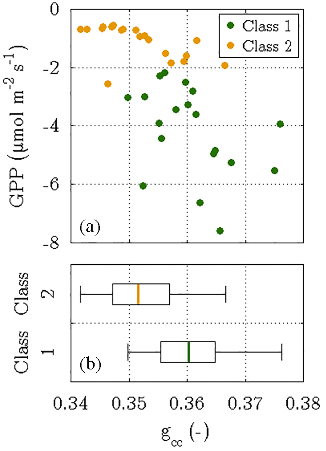
Figure 9Outcome of the phenocam approach, i.e. determining the green chromatic coordinates (g_cc) of two target areas in time-lapse images that were taken between 18 June and 6 July 2014. The g_cc values were computed for both vegetation classes and depict the fraction of the green colour in relation to the three primary colours in the RGB colour space. While the scatter plot (a) displays daily means of photosynthesis versus their corresponding g_cc values, the box plots (b) visualise the difference in the distribution of g_cc values between both vegetation classes. The significantly greater greenness in vegetation class 1 was associated with larger photosynthetic rates, whereas vegetation class 2 was characterised by a less green canopy and thus a lower photosynthetic activity (P<0.05).

Download

Secondly, during periods with a certain wind direction and atmospheric stability, the fetches of some observed fluxes were strongly dominated by only one vegetation class as opposed to the commonly mixed signals. Thus, observed fluxes that are accompanied with a large contribution of one vegetation class (Ω>0.7) were compared to fluxes that were modelled for the same vegetation class. The choice of an Ω of 70 % rested in the desire to identify a trade-off between both applying many fluxes for a broad statistical basis (low Ω) and utilising many fluxes without a mixed fetch for an accurate evaluation (large Ω). Both observed and modelled fluxes match very well as indicated by a mean R² of 0.88 and a mean RMSE of 0.82 µmol m⁻² s⁻¹. When MAE is applied as an intuitive error metric, the decomposed fluxes are associated with a mean error of roughly 0.56 µmol m⁻² s⁻¹. The frequent similarity of the vegetation-class-specific flux rates, however, reduces the effectivity of this validation test. Therefore, the observed fluxes governed by one vegetation class were also compared to fluxes modelled for the other class. This counter-check caused a rise in mean RMSE and MAE by 89 % and 99 %, respectively, thus lending further credibility to the modelled flux rates. It can be assumed that this rise would be far greater if the flux rates of both vegetation classes were less similar.

Thirdly, closed chamber measurements have been carried out with an opaque chamber during mid-June 2014 in vegetation class 2 east of the flux tower (Benjamin Runkle and Alex Sabrekov, personal communication, 2016). Similar to the respiration modelled for this class, a mean carbon dioxide flux with a standard deviation of 2.1±0.9 µmol m⁻² s⁻¹ was observed. This mean, however, is based on five individual discontinuous chamber measurements and thus conclusive to only a limited extent, since taking the spatial variability into account is crucial, when fluxes are scaled between eddy covariance and chamber measurements (Oechel et al., 1998). Chamber measurements have also been conducted in vegetation class 1 but only to the exclusion of shrubs due to their chamber-incompatible size.

Fourthly, the discussion of the obtained fitting parameters and their comparison with values estimated at other sites gives further confidence in the validity of the decomposed fluxes (Figs. 6 and 7):

• The estimated R_base values follow a temperature-driven seasonal cycle, in which R_base,2 is mostly lower than R_base,1. A smaller autotrophic respiration can be attributed to the lesser biomass of the sedges, and a smaller heterotrophic respiration can be ascribed to both increased soil moisture and decreased soil temperature, which in turn hamper microbial activity in the depressions (Hobbie et al., 2000; Walz et al., 2017). For comparison with values found at other sites, a mean peak season TER was computed for vegetation class 1 (2.8 µmol m⁻² s⁻¹) and vegetation class 2 (2.3 µmol m⁻² s⁻¹). While the latter respiratory rate corresponds to the mean mid-growing season TER of 2.2 µmol m⁻² s⁻¹, which was estimated for northern peatlands, the former rate is greater (Frolking et al., 1998; Laurila et al., 2001). The comparatively large respiration in vegetation class 1 is likely due to both the large willow shrubs (fostering autotrophic respiration) and the large active layer depth (facilitating heterotrophic respiration).

• The estimated Q₁₀ values of 1.42 and 1.48 are well within the range of 1.3≲Q₁₀≲1.5, which was retrieved across different ecosystems and climates (Mahecha et al., 2010). Furthermore, the fact that Q_10,1 was lower than Q_10,2 is in accordance with a concept, which suggests a correlation between a lower/greater soil temperature sensitivity and a drier/wetter tundra (Olefeldt et al., 2013).

• The estimated P_max values also follow a seasonal course reflecting the growth and senescence of the canopy. The reason for $P_{max,\mathrm{1}}$ being greater than $P_{max,\mathrm{2}}$ is the larger biomass of the bushes relative to the sedges. The values agree well to the maximum assimilation rates of approximately 15.9 and 11.1 µmol m⁻² s⁻¹ that are, respectively, found for Salix pulchra and Carex aquatilis during the peak of the Arctic growing season (Oberbauer and Oechel, 1989; Tieszen, 1975). Given a mean mid-growing season P_max of 8.6 µmol m⁻² s⁻¹ for northern peatlands, $P_{max,\mathrm{2}}$ (8.9 µmol m⁻² s⁻¹) constitutes a representative uptake capacity, whereas $P_{max,\mathrm{1}}$ (12.3 µmol m⁻² s⁻¹) suggests a comparatively large potential for sequestering carbon dioxide (Frolking et al., 1998; Laurila et al., 2001). Another aspect that indicates the reliability of the estimated P_max values is their relationship with the NDVI as seen at many other tundra ecosystems (Mbufong et al., 2014; Shaver et al., 2007). Regarding both growing seasons, the footprint's NDVI was greater in 2015, suggesting a more active vegetation than in 2014 (ORNL, 2017). Similarly, the P_max values of both vegetation classes, in particular the values of the more abundant vegetation class 2, were greater during 2015. Satellite records for tundra landscapes are, however, often confounded by various effects that are particularly profound in high-latitude regions (Stow et al., 2004). Therefore, satellite-derived NDVI values of tundra ecosystems may need to be double-checked with optical sampling in the field, if they are applied to resolve interannual differences (Gamon et al., 2013).

• The estimated α values amount to 0.042 (α₁) and 0.04 (α₂), and are thus greater than the mean mid-growing season α of northern peatlands amounting to 0.023 (Frolking et al., 1998; Laurila et al., 2001). The high light sensitivity indicates an efficient physiology enabling a considerable photosynthetic activity at low irradiance levels. The ratio between the α values of both vegetation classes is similar to the ratio of quantum yields that were compiled from tundra landscapes in Alaska and Sweden during the Arctic peak season: 0.038 for Salix spp. and 0.03 for Carex spp. (Shaver et al., 2007).

4.3 Interpretation of diurnal, seasonal and interannual flux variabilities

On the diurnal scale, the temporal variability in the carbon dioxide fluxes was controlled by meteorological conditions. For comparison among climate-relevant trace gases at this site, the methane fluxes exhibited a larger temporal variability, which was rather governed by the spatial variability, i.e. the constantly varying source area composition in the fetch (Rößger et al., 2019a). On the interannual scale, the carbon dioxide fluxes displayed, in contrast to methane fluxes, a larger variability, which was driven by typical abiotic factors such as snowmelt timing and initial growing season temperatures (Aurela et al., 2004; Groendahl et al., 2007). Due to the inhomogeneous surface, however, biotic factors such as canopy structure and distribution also provide explanatory power.

In 2015, the rapid snowmelt coincided with the spring flood, thus enabling both vegetation classes to commence their canopy development concurrently in early June. The growing season was initialised in mid-June by mosses, which are much more abundant in vegetation class 2 (Fig. 8). Mosses are, in contrast to vascular plants, able to start assimilating right after snowmelt since their photosynthetically active tissue can be maintained over winter (Oechel, 1976). From this point until late September/early October, mosses formed a basal net uptake. Considerable moss activity until late autumn has also been observed on the nearby river terrace (Eckhardt et al., 2019; Kutzbach et al., 2007b). Furthermore, mosses can account for distinctly more than half of total photosynthesis, as demonstrated for graminoid areas with high moss cover (Douma et al., 2007; Sommerkorn et al., 1999). However, it is possible that mosses did not fully photosynthesise throughout the growing season due to their tendency to lower their photosynthetic capacity under high irradiance (Murray et al., 1993). This light stress depends on cloudiness, solar altitude, moss structure and shadowing by vascular plants, altogether promoting a late-season activity of mosses while other plants were already dormant (Zona et al., 2011). On top of the basal moss activity, the shrubs of vegetation class 1 exhibited a larger net uptake until the growing season peak around late July/early August, after which the sedges of vegetation class 2 dominated the carbon dioxide exchange. The fact that Carex spp. started growing earlier than Salix spp. has also been observed at other sites; however, considerable variation exists in the timing of phenological events both among and within species (Chapin et al., 1992; Wielgolaski et al., 1975).

In 2014, air temperatures were higher than the monthly long-term means throughout the measurement period (Fig. 4). During the early and slow snowmelt in mid-May, the low sedges and mosses remained buried in the depressions with accumulated snow longer than the large bushes on the elevated ridge with less snow. Thereby, the willow twigs were exposed to daytime temperatures above freezing leading to the development of catkins in late May already. Hence, vegetation class 1 was more advanced in its phenology than vegetation class 2 at the onset of the growing season. The consequence was the substantially larger net uptake of the shrubs until the seasonal peak in early August. Apparently, the shrubs largely benefitted from elevated early growing season temperatures, an effect that has also been found favourable for shrub encroachment in the Arctic (Myers-Smith et al., 2011). Incidentally, shrubs have been growing on Samoylov Island only since the 1960s (Eva-Maria Pfeiffer, personal communication, 2017). Besides the delayed phenological development, the low carbon sequestration of vegetation class 2 during that period can also be attributed to a soil moisture deficit-induced decline in net assimilation of mosses, as they are prone to desiccation due to both missing roots and the absent ability to actively regulate their internal water content (Turetsky et al., 2012). Similar to the other year, vegetation class 2 dominated the net uptake after the growing season peak, in particular during late August, which can likely be ascribed to enhanced moss activity.

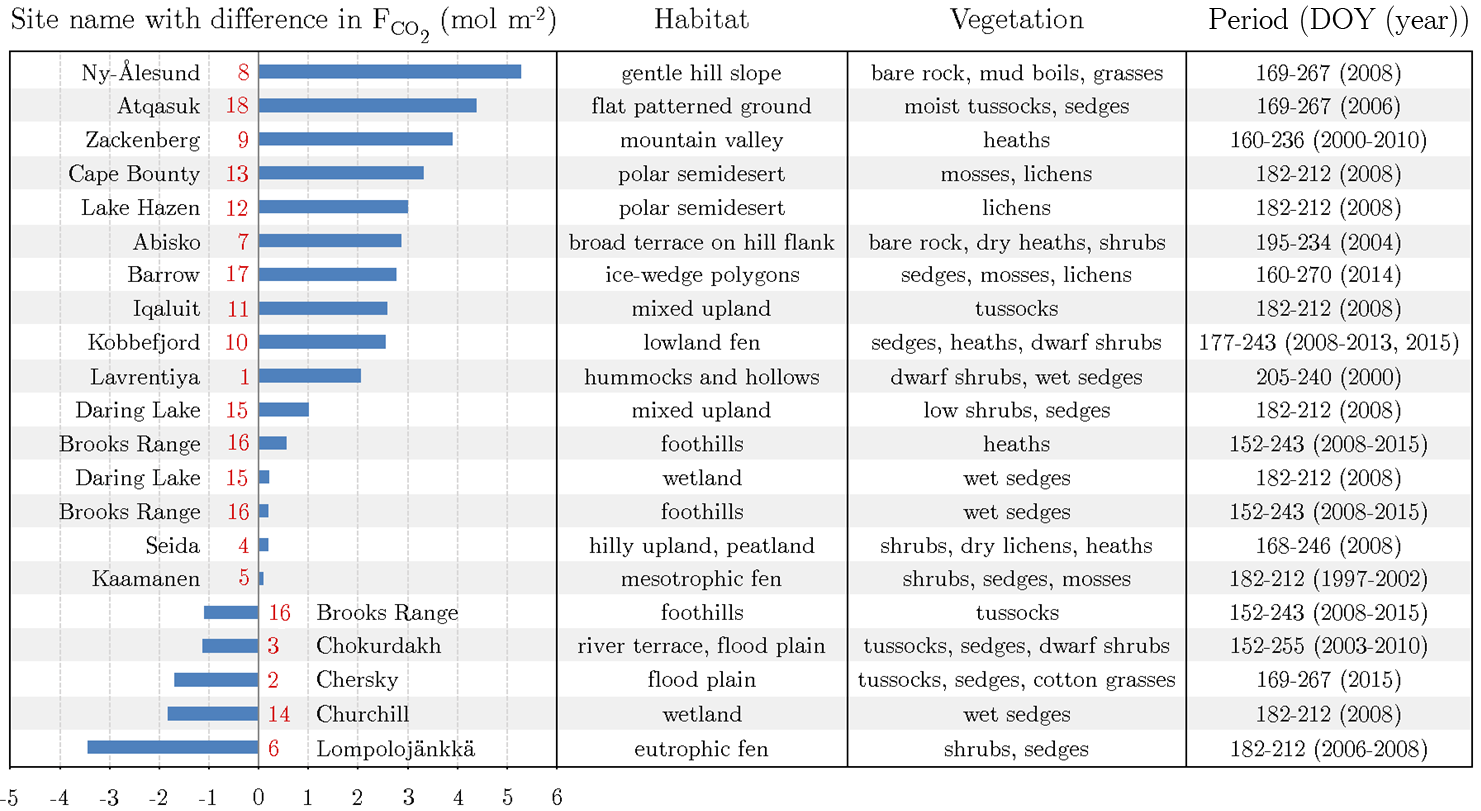
Table 3Putting the carbon dioxide budgets of the flood plain in perspective with budgets estimated by means of the eddy covariance method at other Arctic sites. A negative/positive difference in the budgets indicates a carbon dioxide sink strength of the comparison site being greater/lower than the one of the flood plain on Samoylov Island. For an appropriate comparison, the budgets of this study's site were recomputed for the day of the year (DOY) periods of the other sites. In this process, representative 2015 flux data were basically utilised, unless the budget of the other site derived from 2014. If the budget period of the other site exceeded the period of this study’s budget, the (few) missing days in the start/end were filled with the daily sum of the first/last day in the budget period. The numbers next to the bars refer to the numbers in the circumpolar map (Fig. 1). Compared to various Arctic sites, the flood plain on Samoylov Island constitutes a distinctly strong carbon dioxide sink.

Download Print Version

4.4 Appraisal of the budgets' representativeness

The spatial representativeness of the observed fluxes can be assessed with the sensor location bias (Schmid and Lloyd, 1999). If the flux rates of the considered surface classes are similar, as in 2015, the deviation between the respective surface class compositions in footprint and area of interest plays a minor role (Table 1). In 2014, the sensor location bias came into effect as the flux decomposition unveiled a varying seasonality between both vegetation classes that was concealed in the net signal. In this case, a quantitative comparison of the flux budgets with other sites lacks validity due to a potentially non-representative surface class composition; i.e. the comparison of the flood plain's greenhouse gas budgets with the budgets of the river terrace must remain restricted to Samoylov Island and cannot be extended on the Lena River Delta (Table 2). The revealing outcome of the flux decomposition proves its utility for an enhanced interpretation of eddy covariance data by gaining insights into the phenological dynamic of individual vegetation classes. It also demonstrates that climatologically unusual conditions can adversely affect the representativeness of the footprint, resulting in the potential need to regularly examine the representativeness of apparently homogeneous footprints, in particular during prolonged unusual weather conditions as biased budgets may otherwise be estimated.

The temporal representativeness of the obtained budgets may thus be constrained on the interannual scale. As the air temperatures in 2015 better correspond to long-term means than in 2014, the 2015 budgets are better suited for an intersite comparison (Table 3). Moreover, the obtained budgets also possess a confined validity on the annual scale since they only cover a period that is similar to the growing season. Outside this period, no uptake of carbon dioxide occurs, implying a lower year-round sink strength for greenhouse gases. This assumption is based on the accumulating evidence that the release of carbon dioxide and methane is not negligible during the very cold winter – in contrast to the traditional view of a wintertime inactivity in Arctic ecosystems (van der Molen et al., 2007). For instance, at multiple sites in Alaska, the cold season release of carbon was found to equal 1–2 times the warm season net uptake (Euskirchen et al., 2012; Oechel et al., 2014; Zona et al., 2016).

4.5 Comparison of the budgets with other Arctic sites

Across various Arctic flux sites, the flood plain of Samoylov Island exhibits a carbon dioxide sink strength that is distinctly greater than the average (Fig. 1 and Table 3). This aspect appears noteworthy when local conditions are taken into consideration: the mean net radiation during the growing season is lower than for most Arctic sites, and the underlying permafrost displays one of the lowest ground temperatures in the world (Boike et al., 2013; Obu et al., 2018; Romanovsky et al., 2010). The diminishing effects of these climate factors are counterbalanced by the deposition of nutrients in the course of spring flooding (van Huissteden et al., 2005). Among the three great Siberian rivers draining into the Arctic Ocean (Ob, Yenisei, Lena), the Lena River ranks first in terms of total suspended matter (Cauwet and Sidorov, 1996). A large portion of this matter is transported during the annual spring flood, thereby regularly mitigating the nutrient limitation that affects many Arctic ecosystems (Beermann et al., 2014; Fedorova et al., 2015).

More specifically, the net uptake of the flood plain on Samoylov Island is distinctly weaker compared to flood plains of the Siberian rivers Kolyma and Indigirka (Kittler et al., 2017; Parmentier et al., 2011). Other Siberian sites encompass Seida and Lavrentiya, which exhibit a similar and stronger net uptake, respectively (Marushchak et al., 2013; Zamolodchikov et al., 2003). Furthermore, the flood plain's net uptake is considerably stronger than budgets of high Arctic sites in Svalbard, Greenland and Canada (Lafleur et al., 2012; López-Blanco et al., 2017; Lüers et al., 2014; Lund et al., 2012). In comparison with sites in either the low Arctic or sub-Arctic, no general conclusions can be drawn, which is likely due to the ubiquitously high spatiotemporal flux variability in the Arctic region. Also, no uniform picture emerges in comparison to Scandinavian peatlands (Aurela et al., 2002, 2009; Fox et al., 2008). Compared with sites in the northern part of the north slope of Alaska, the flood plain exhibits a substantially stronger net uptake (Oechel et al., 2014; Raz-Yaseef et al., 2017); in the southern part, however, similar net uptakes seem to prevail (Euskirchen et al., 2016).