2.1 Site and data

2.1.3 Mapping of landscape characteristics

The land cover classification consists of nine classes visually distinguished according to their key characteristics (Table 1). The LCCs were identified within an area of 1 km² around the EC tower on the basis of a vegetation and soil survey and verified using statistical ordination of the 92 established study plots according to plant species composition and functional plant and soil attributes (Mikola et al., 2018). To extrapolate the LCCs to the landscape scale (Figs. 1a and S2), a supervised object-based classification with the random forest method was carried out using two VHSR multispectral satellite images (12 August 2012 and 11 July 2015; WorldView-2, DigitalGlobe, Inc., Westminster, CO, USA) and a digital elevation model (DEM) constructed from the 2015 WorldView-2 stereo pair (Fig. 1b). The internal (cross-validation of training data) and external (validation data) classification accuracies of the land cover classification were 80 % and 49 %, respectively. For details, see Mikola et al. (2018).

Table 1Land cover classes and their dominating vegetation and other characteristics, derived from Juutinen et al. (2017) and Mikola et al. (2018).

Download Print Version | Download XLSX

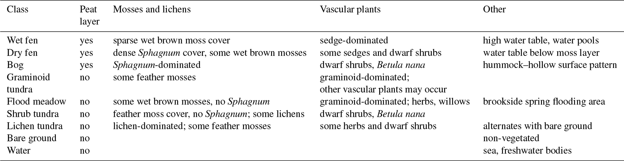
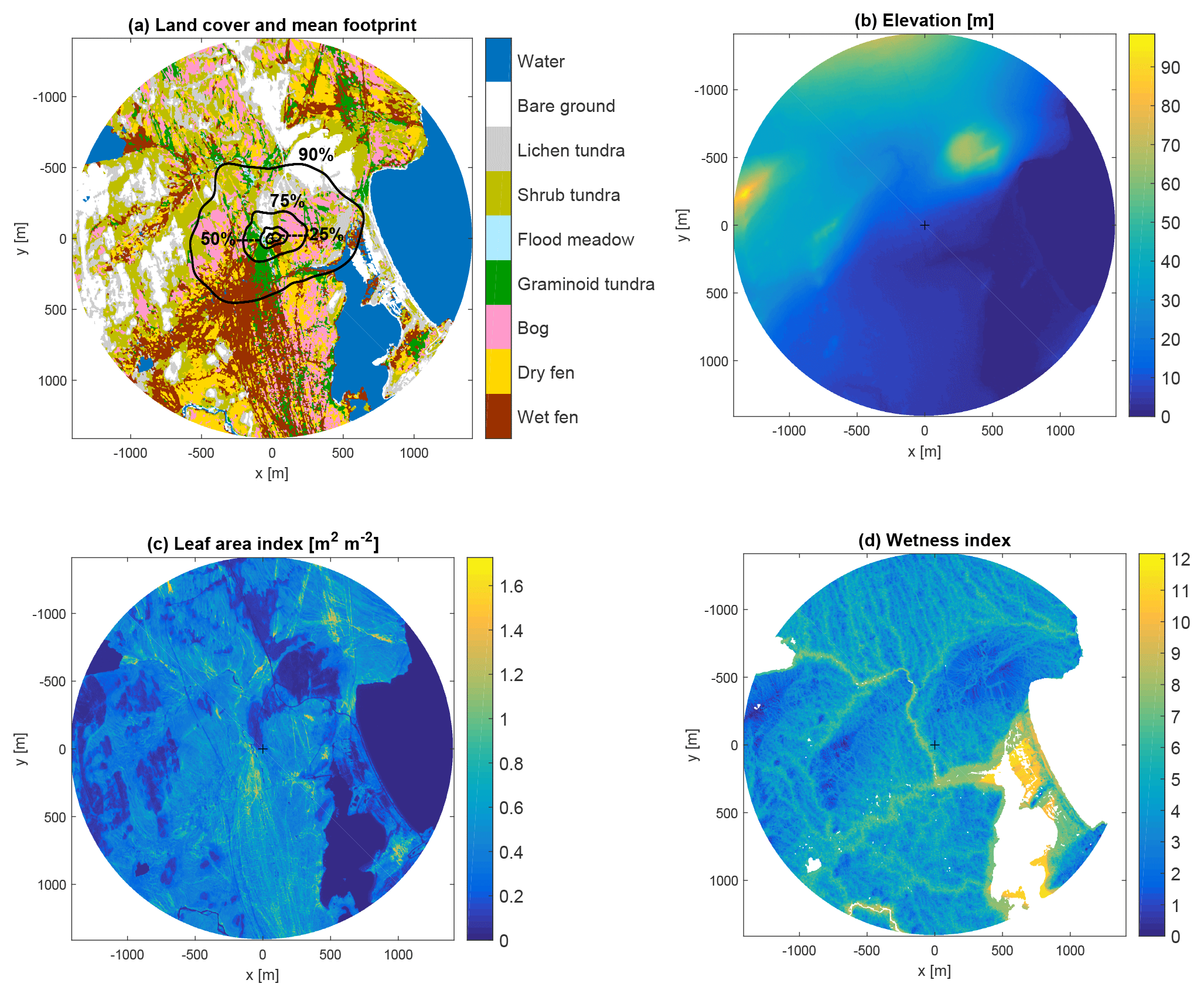
Figure 1Land cover classes and the mean cumulative footprint during the growing season of 2014 (a), terrain elevation (b), maximum leaf area index (on 12 August 2012) (c) and topographic wetness index for terrestrial surfaces (d). The isopleths in panel (a) indicate the areas with a 25 %, 50 %, 75 % and 90 % contribution to the measured flux (only the further distance visible). The plus sign indicates the location of the EC tower.

Download

Using non-linear regression, the LAI of vascular plants was estimated from the normalized difference vegetation index (NDVI) calculated from the reflectance data of the 2012 WorldView-2 image (Fig. 1c). This map represents the period of maximum LAI in 2012; for the estimated development of the LAI of different LCCs in 2014, see Juutinen et al. (2017) and Fig. S1. The topographic wetness index (TWI) was calculated from the DEM using the method of Böhner and Selige (2006) (Fig. 1d). TWI is defined as a function of the upslope contributing area and the local terrain slope and thus serves as a proxy for potential soil moisture. For details of the DEM and TWI data, see Mikola et al. (2018). All maps have a 2 m pixel size, and in this study they were limited to a circle with a radius of 1.4 km from the EC tower, which defines the domain of the present study. For upscaling to a regional scale, we also considered the LCCs determined within a larger area of 35.8 km² (Fig. S2).

2.2 Application of footprints

2.2.3 Examples of flow conditions

To demonstrate how the EC flux measurement in Tiksi is affected by surface heterogeneity, we calculated the footprint-weighted averages of the surface attributes LAI, terrain elevation and TWI using Eq. (2) and the data illustrated in Fig. 1b–d as the continuous variable X, while Eq. (5) was used for the footprint-weighted LCC areas of the nine classes shown in Fig. 1a. For this demonstration, we defined three flow situations in terms of the variables that affect the footprint in a given θ, i.e. U, u_*, L⁻¹ and σ_v (Table 2). These cases represent differing stability conditions, for which typical parameter combinations were derived from the measurement data employed in this study. The U–u_*–L⁻¹ combination was constrained by z₀=0.01 m as calculated from the MOS profile of the horizontal wind speed (Pasquill and Smith, 1983). For lateral wind velocity fluctuations, which only affect turbulent diffusion in the crosswind direction, we used the scaling ${\mathit{\sigma }}_v/u_{*}=\mathrm{2.3}$. This corresponds to the median of our data and, for simplicity, was adopted here for all stabilities.

Table 2Flow conditions assumed for the example calculations.

Download Print Version | Download XLSX

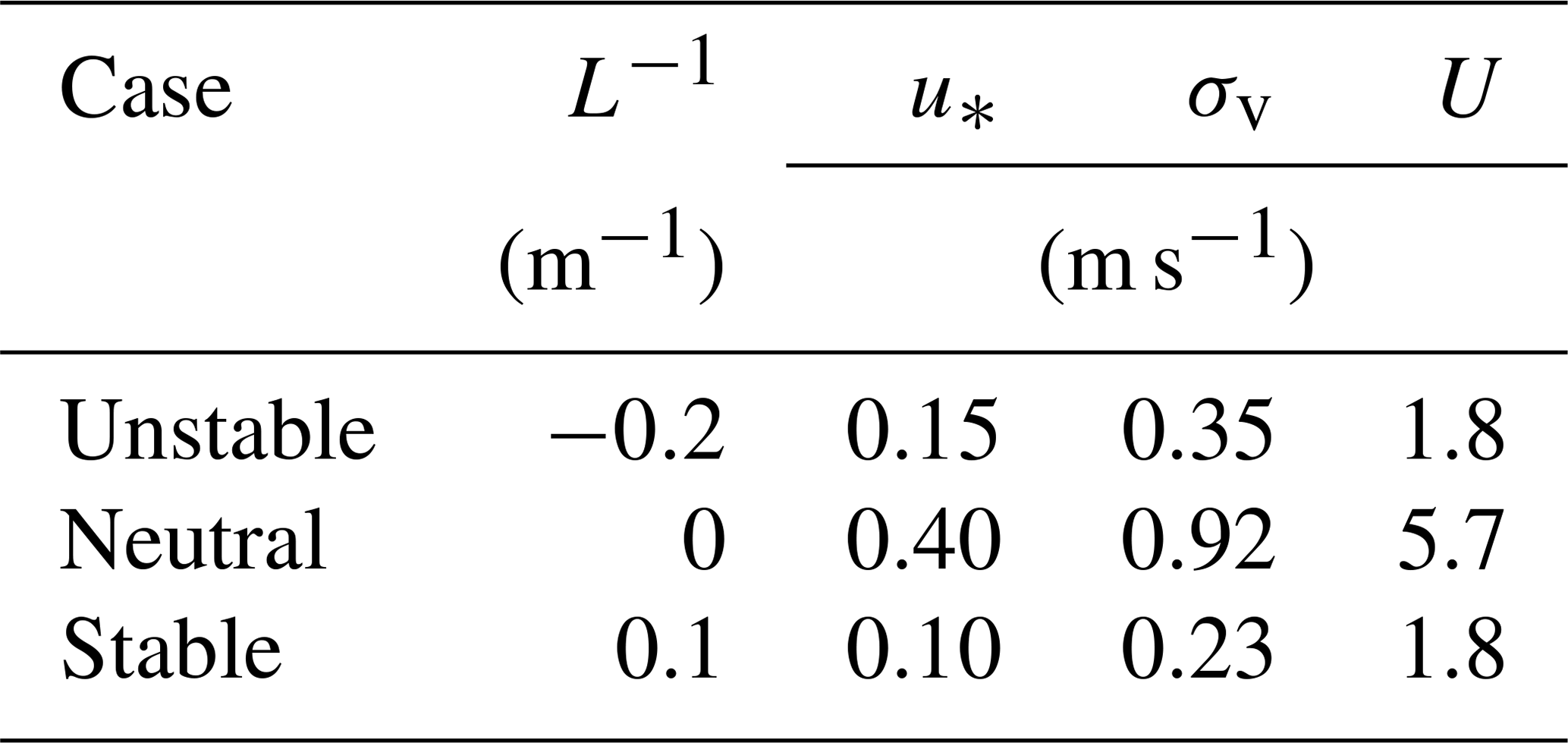
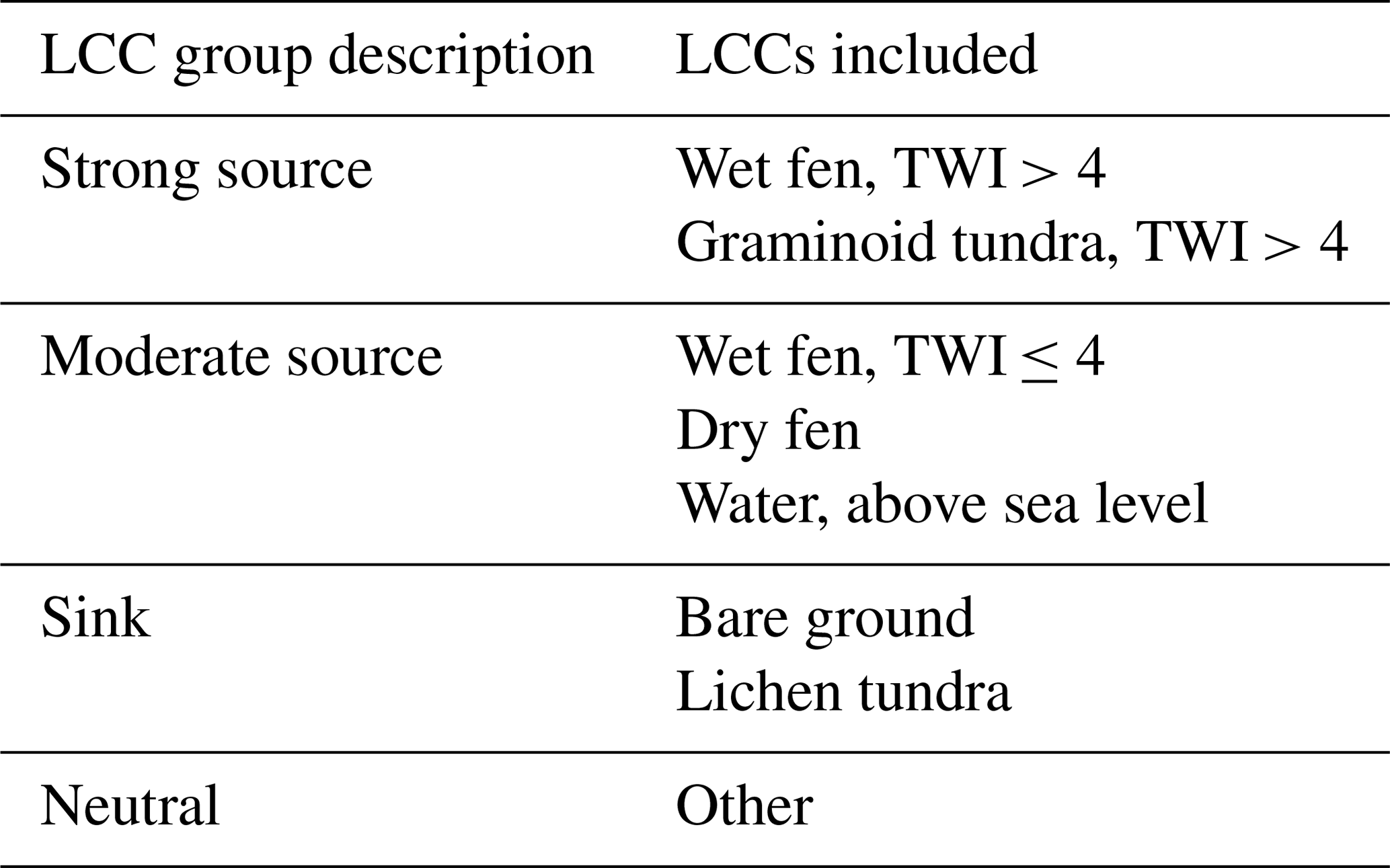
Table 3Aggregated land cover classes for the regression model.

Download Print Version | Download XLSX

2.3 Statistical model

2.3.1 Land cover class aggregation and upscaling of CH₄ fluxes

We hypothesize that mean CH₄ fluxes can be determined for LCC groups, each composed of LCCs of similar expected source–sink capacity. This grouping was based on the documented vegetation and soil characteristics, reported in detail by Mikola et al. (2018) and Nyman (2015), and summarized here in Sect. 2.1.4. In addition, we utilized the TWI map and defined areas of potentially wet soils as those with TWI >4 (Fig. 1d). Using these data and syntheses of CH₄ production and fluxes in similar ecosystems (Olefeldt et al., 2013; Nicolini et al., 2013; Turetsky et al., 2014; Lau et al., 2015; Petrescu et al., 2015; Treat et al., 2015) as background information, we defined four aggregated classes (Table 3, Fig. 2), for which the LCC group-specific fluxes were determined with the statistical model described below (Sect. 2.3.2).

Figure 2Distribution of the aggregated land cover classes (excluding marine areas).

Download

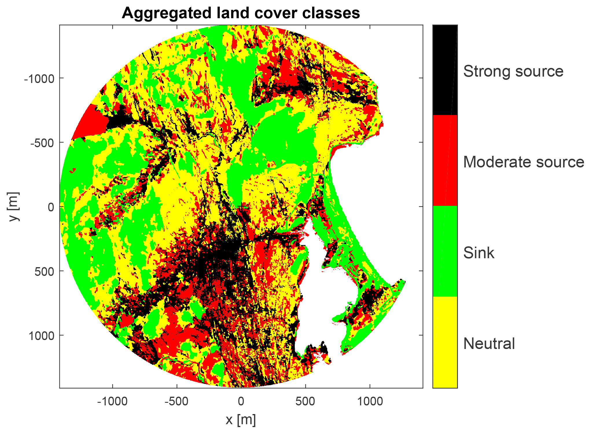
The data sources listed above suggest that wet fens typically are strong CH₄ emitters, and thus the pixels of the wet fen LCC with TWI > 4 were selected for the first LCC group (“strong source”; Table 3). We also assumed that the pixels of the graminoid tundra LCC in the potentially wet locations should be included in this category as the graminoids at the site are dominated by aerenchymatous Carex spp. and Eriophorum spp. (e.g. E. vaginatum), i.e. plants known to be associated with substantial CH₄ emissions. The drier fens within the study area likely act as weaker emitters, so these were combined into another LCC group (“moderate source”), together with the bodies of freshwater (water LCC above the sea level). The syntheses cited above also justify an assumption that mineral soils, i.e. here the bare ground and lichen tundra LCCs, act as weak CH₄ sinks (“sink”). The proportional areas of these three LCC groups were used as the explanatory variables in the regression model. The remaining pixels were allocated to the fourth group consisting of the LCCs that either are expected to have a very small CH₄ flux on average or cover only a limited area in flux footprints (“neutral”). This group is included as an intercept in the regression model, and we hypothesize that its estimated value is not statistically different from zero.

The CH₄ fluxes determined for the aggregated LCCs defined above were upscaled by a simple mosaic approach, i.e. by areal weighting of the group-specific fluxes. To illustrate how the upscaled flux depends on land cover heterogeneity at different spatial scales, the upscaling was performed for different subdomains as a function of the distance from the EC tower, and also for a larger area of 35.8 km² (Fig. S2).

3.1 Demonstrating surface heterogeneity

Our footprint analysis shows that those surface elements that had the greatest influence on the EC measurements in Tiksi were typically located within a distance of 10–200 m (Table S1 in the Supplement). However, the actual range depended strongly on atmospheric stability, as expected (Horst and Weil, 1992). The distance of maximal influence in a single footprint varied from 18 to 35 m depending on stability, and the estimated far end of the source area ranged from 200 to 3500 m for the 90 % flux contribution, for instance. The 1.4 km radius of the circle centred at the EC tower, which defines our primary study area, was selected to result in a 95 % footprint coverage within this area in the neutral case. About 15 % of the footprint calculated for the stable flow example extended beyond the limits of this area, while in the unstable case 99.7 % of the footprint was confined to the target circle (Fig. 3).

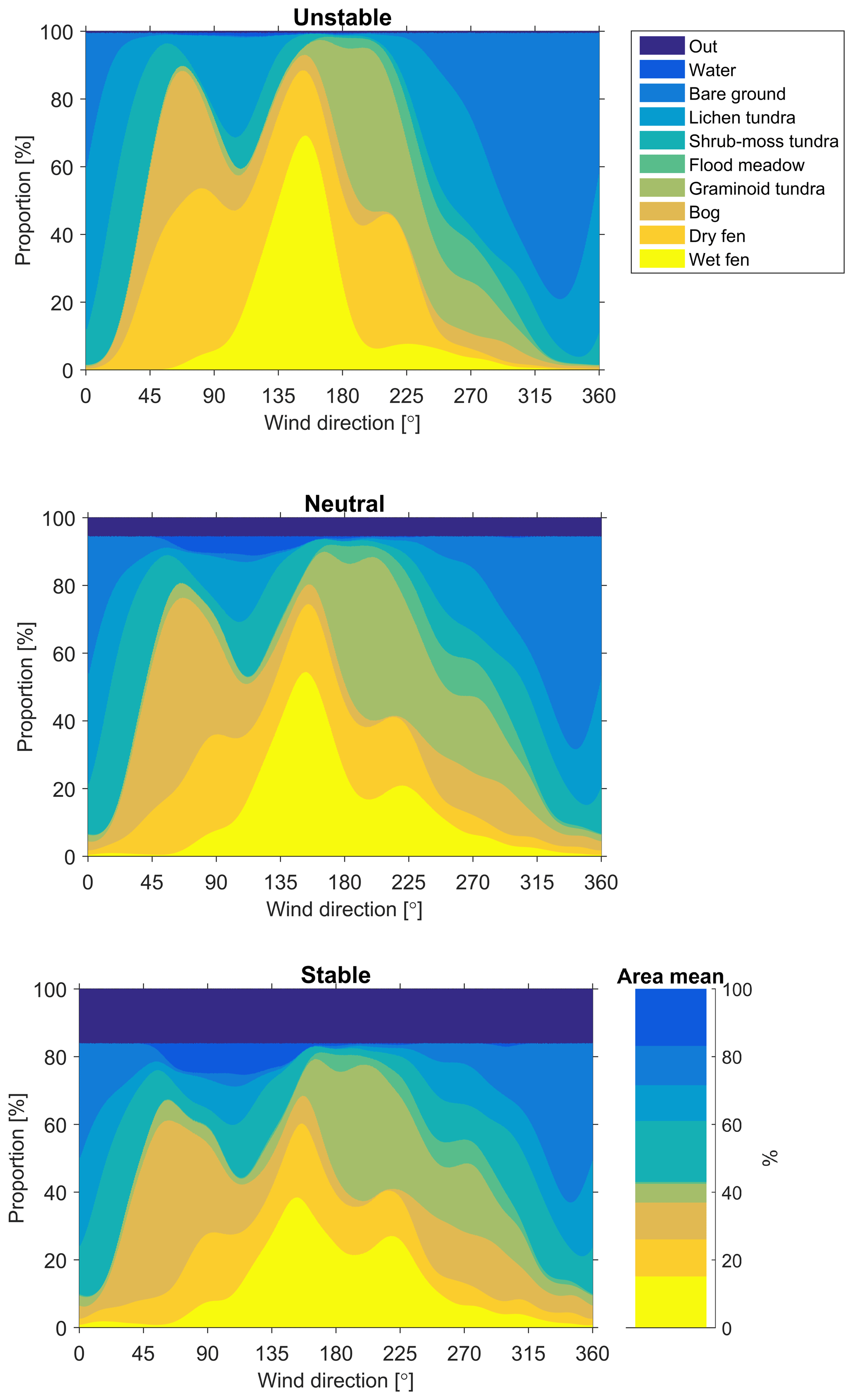
Figure 3Proportion of different land cover classes in the flux footprint as a function of wind direction for the three flow condition cases specified in Table 2. The rightmost panel shows the relative coverage of these classes within the study area.

Download

The variation of the footprint-weighted LCC contributions, calculated with Eq. (5), as a function of wind direction demonstrates how the heterogeneity inherent in tundra landscape manifests itself in the EC measurement data (Fig. 3; see also Fig. S3). As is obvious from the LCC map (Fig. 1a), the distribution of contributing LCCs varied a lot among different wind directions (Fig. 3). In the neutral case, for example, there were seven different LCCs dominating at least in one sector. Turbulent mixing also played a substantial role in the magnitude of relative LCC contributions, as the weighting of longer distances increased with increasing stability. In some directions, the contribution of the most common LCCs was highly sensitive to atmospheric stability. In the north-east-to-east sector, for example, the relatively small dry fen patch located within a few tens of metres from the EC tower (Fig. 1a) contributed 45 % in the unstable case but only 13 % in the stable case (Fig. 3). Similarly, the relative importance of the extensive bare-ground area between the west and the north-east strongly depended on atmospheric stability.

The footprint-weighted surface characteristics, calculated with Eq. (2) for the cases detailed in Table 2, further demonstrate the landscape heterogeneity-induced variations. The effective LAI originating from the footprint-weighting of the LAI map showed a strong dependency on wind direction: in the neutral case, for example, 〈LAI〉 ranged from 0.19 to 0.64 m² m⁻² (Fig. 4a). In the unstable case, the direction dependency was similar; however, 〈LAI〉 was up to 0.12 m² m⁻² lower than in neutral conditions due to the dominance of bare ground in the vicinity of the EC tower in the north-western sector (Fig. 1a). As averaged over all directions, here assumed equally frequent, 〈LAI〉 was in all stability cases somewhat higher than the arithmetic areal average (Fig. 4a). Due to the directional variations in 〈LAI〉, the maximum sensor location bias (Δ_LAI, Eq. 6) may exceed 90 % in the direction of the maximum 〈LAI〉.

Figure 4The footprint-weighted and areally averaged leaf area index (a), terrain elevation (b) and topographic wetness index (c) as a function of wind direction for the three flow condition cases specified in Table 2. The right-hand ordinate indicates the corresponding sensor location bias.

Download

Based on a corresponding footprint-weighting, an effective mean value could also be determined for terrain elevation (Fig. 4b). This shows that, even though the topographic variability within the flux footprint was small, slightly different terrain elevation patterns are associated with each flux measurement depending on both wind direction and stability. The sensor location bias for elevation was negative in almost all flow conditions, as the elevation is on average lower within the area that typically dominates the flux footprint (Figs. 1b and 4b). The area of predominantly bare ground was also apparent in the effective TWI (Fig. 4c). In the east-to-south sector, the differences between the stability classes are due to the higher TWI values determined along the coast (Fig. 1d) that gain in importance in stable conditions. Between the south-west and the north-west, in contrast, 〈TWI〉 was higher in unstable conditions, which results from the more pronounced influence of the brook running near the EC tower. The footprint-weighted TWI averaged over all directions was, in all cases, close to the arithmetic area average, with the magnitude of the corresponding Δ_TWI being lower than 30 % (Fig. 4c).

In addition to the examples presented above, we demonstrated the heterogeneity of the Tiksi landscape by calculating the mean LAI and LCC contributions from the time series of EC measurements adopted for the present analysis. Figure 1a shows the footprint climatology for the growing season of 2014, depicted as the smallest bounded region containing the surface elements that contribute to EC measurements by a certain fraction (Eq. S1 in the Supplement). This source area is clearly asymmetric, and comparison with the data in Table S1 indicates that the source area is more limited than the corresponding area in typical neutral conditions; i.e. it effectively reflects slightly unstable conditions. Weighting the LAI distribution by the mean footprint resulted in a bias of Δ_LAI=20.2 %. For comparison, this is much larger than the bias in the NDVI estimated for EC sites in northern China: at the 1 km² scale, Δ_NDVI ranged from −6.9 % to 4.2 % at eight sites with low vegetation, and even at a land model scale of ∼300 km² the mean absolute Δ_NDVI was not more than 6.5 % (Wang et al., 2016). Notwithstanding such a high degree of agreement, one of the sites was considered “disturbed”. In another study, the EC measurements at two sites with a Δ_NDVI of less than 4 % reported for the 1 km² scale were considered unbiased, while a Δ_NDVI of 28 % determined for a grassland site was judged as problematic; the mean NDVI, and hence Δ_NDVI, was very similar up to the maximum scale of 4 km² investigated (Kim et al., 2006).

For most of the LCCs in Tiksi, the field of view of the EC sensors averaged over the growing season clearly differed from the areal coverage of the LCCs within the study area (Table 4; see also Fig. S4 for the effect of wind direction and stability). Here, we have excluded the large marine areas, which have a minor weight in the EC data. The difference is still largest for the water LCC, as the freshwater bodies are concentrated on the fringes of the study area, and for the flood meadow category with a limited coverage. However, there were also major differences among the dominating terrestrial classes, such as shrub tundra and wet fen: the surface elements attributed to these LCCs contributed to the EC observations less (by 40 %) than their total areal coverage would suggest.

Table 4Proportions (%) of different land cover classes as weighted by the mean footprint function during the growing season (“weighted”) and their areal coverages within the study area (“area”), within the source area defined by the 90 % cumulative footprint (“area, 90 %”, Fig. 1a) and within a 35.8 km² region (“region”, Fig. S2). The marine areas are excluded, and the integrated footprint within the study area is scaled to 100 %.

Download Print Version | Download XLSX

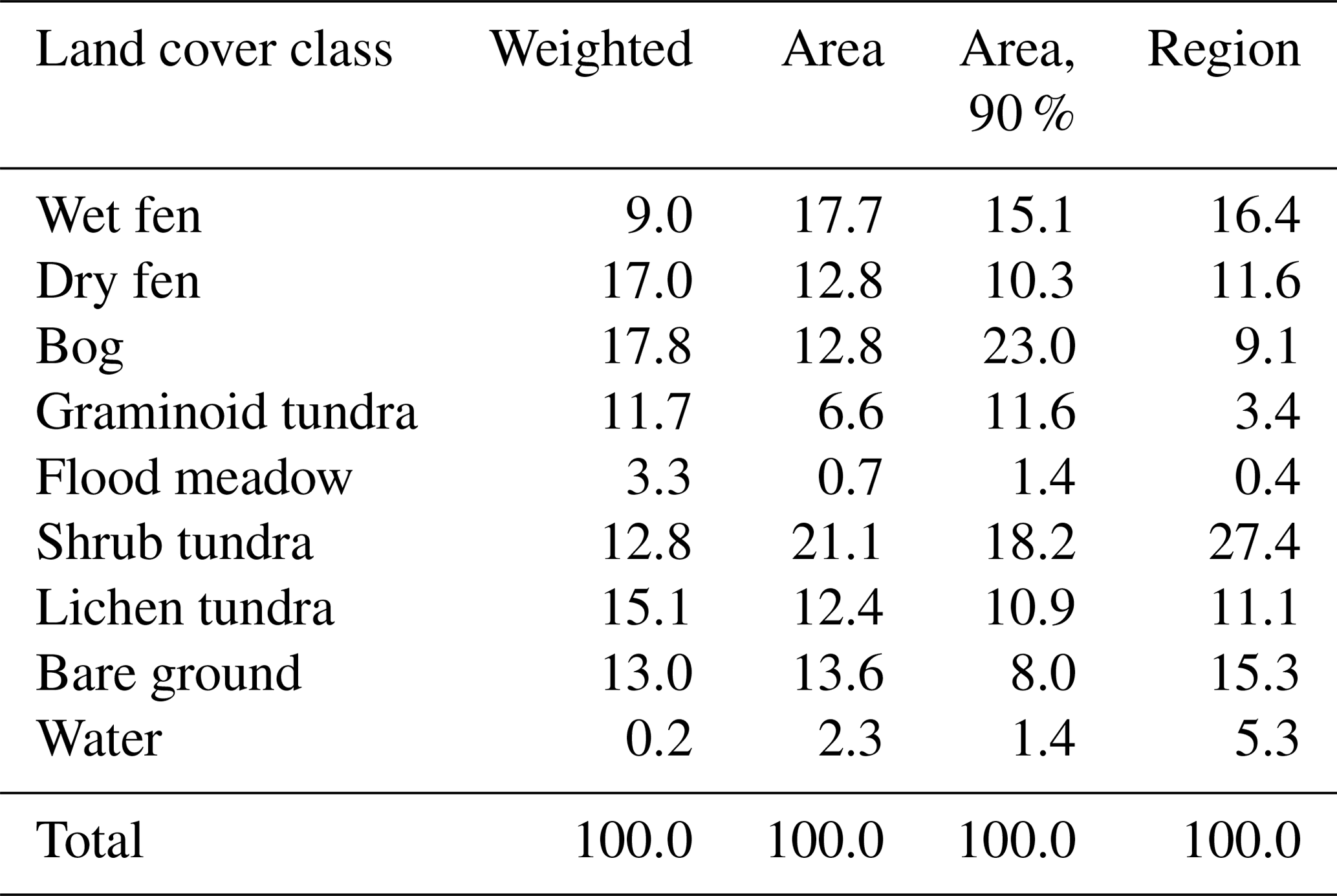
If the areal LCC proportions were calculated within the non-circular area defined by the 90 % cumulative footprint (Fig. 1a), some of these proportions changed dramatically (Table 4). We also included in the comparison the LCC distributions for a 35.8 km² area (Fig. S2). Compared to this, the study area has a similar coverage of fens, bare ground and lichen tundra, whereas the water and shrub tundra LCCs are under-represented and bogs and graminoid tundra over-represented. Overall, these results demonstrate the multiscale heterogeneity of the site and indicate that here the representativeness cannot be described as a proportional coverage of a single target LCC in the footprint climatology, as is the case for most EC sites (Göckede et al., 2008).

3.2 Land cover group-specific CH₄ fluxes

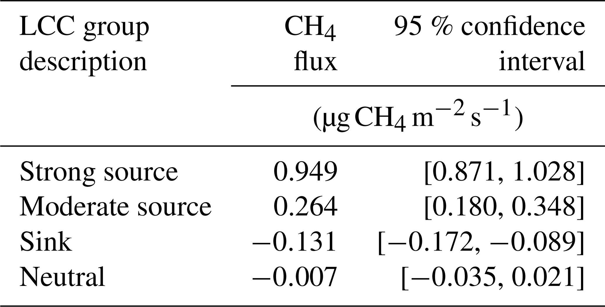
The parameters of the regression model introduced in Sect. 2.3.2 were estimated with OLS for the LCC aggregation presented in Sect. 2.3.1. As this produced model residuals that exhibited both heteroscedasticity and autocorrelation (White LM test statistic $M{R}^{\mathrm{2}}=\mathrm{92}>{\mathit{\chi }}_{\mathrm{0.99}\left(\mathrm{9}\right)}^{\mathrm{2}}$, Breusch–Godfrey LM test statistic $(M-\mathrm{1})R^{\mathrm{2}}=\mathrm{117}>{\mathit{\chi }}_{\mathrm{0.99}\left(\mathrm{1}\right)}^{\mathrm{2}}$), the confidence intervals were based on the Newey–West estimator. Even when these (larger) confidence intervals were introduced, all the estimated parameters except for the constant, i.e. those representing aggregated LCCs with expected CH₄ exchange, proved to be statistically different from zero (p<0.05; Table 5). The results were also in perfect accord with our qualitative hypothesis on CH₄ flux variability among the LCCs: the model could differentiate between the high emitters, moderate emitters and sinks without any explicit prior information on this pattern. Concerning the quantitative differences, Treat et al. (2018) reported the same degree of spatial variation (standard deviation/mean of 155 %) in the modelled annual CH₄ fluxes on low Arctic tundra, highly heterogeneous similarly to Tiksi, and showed that the differences among LCCs clearly dominate over the interannual variation in the regional CH₄ fluxes.

Table 5Estimated CH₄ fluxes for the aggregated land cover classes.

Download Print Version | Download XLSX

The temporal variation of the estimated 30 min ecosystem-scale CH₄ fluxes was consistent with observations, even though it is obvious that the full range of variability, most notably the peak values, could not be reproduced (R²=0.797, RMSE of 0.0994 $\mathrm{\mu }\mathrm{g}{\mathrm{CH}}_{\mathrm{4}}{\mathrm{m}}^{-\mathrm{2}}{\mathrm{s}}^{-\mathrm{1}}$, MAE of 0.0686 $\mathrm{\mu }\mathrm{g}{\mathrm{CH}}_{\mathrm{4}}{\mathrm{m}}^{-\mathrm{2}}{\mathrm{s}}^{-\mathrm{1}}$; Fig. S5). However, part of this variation arose from measurement noise, and in this context it is crucial that the mean fluxes were modelled accurately also when considering the strong wind direction dependence of observations (Fig. 5). Estimated from the mean fluxes of binned data shown in Fig. 5, the variance related to wind direction accounted for up to 80 % of the total variance of measured fluxes. This dependence, obviously generated by the systematic LCC variations within the flux footprint (Fig. 3), is a key pattern in this data set and must be taken into consideration when calculating representative CH₄ balances (Aurela et al., 2015). The model residuals differed significantly (p<0.05) from zero only in a narrow south-eastern wind sector, where the model slightly overestimated the fluxes. The 10-fold cross-validation statistics show that the model performed against independent data only marginally worse than the fit to the full data set (R²=0.794, RMSE of 0.1000 $\mathrm{\mu }\mathrm{g}{\mathrm{CH}}_{\mathrm{4}}{\mathrm{m}}^{-\mathrm{2}}{\mathrm{s}}^{-\mathrm{1}}$, MAE of 0.0691 $\mathrm{\mu }\mathrm{g}{\mathrm{CH}}_{\mathrm{4}}{\mathrm{m}}^{-\mathrm{2}}{\mathrm{s}}^{-\mathrm{1}}$).

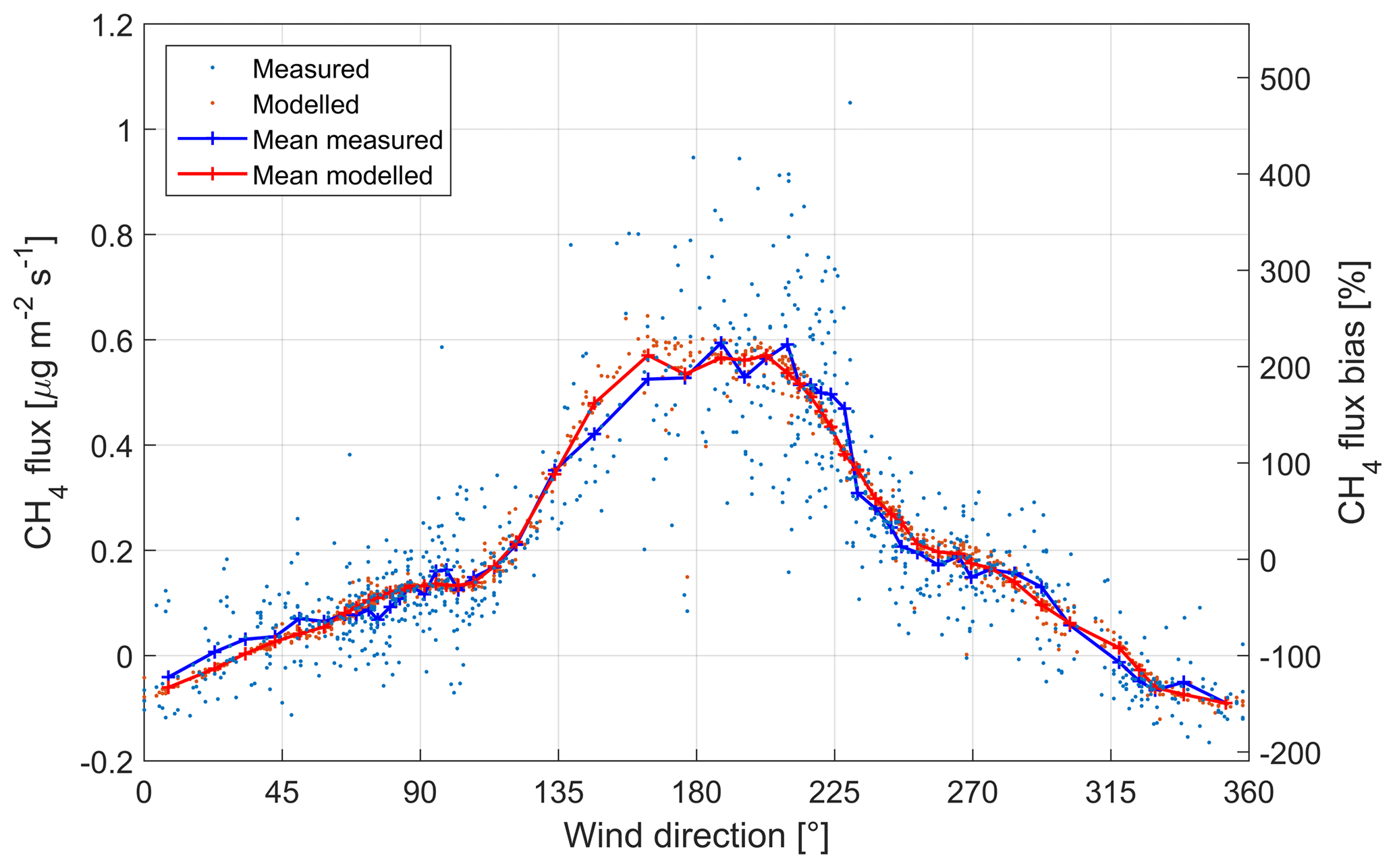
Figure 5Measured and modelled CH₄ fluxes as a function of wind direction (left axis). The averaged data were calculated in 50 direction classes. The right axis indicates the sensor location bias of the measured data shown (both individual points and the mean) with respect to the mean upscaled flux within the study area (0.183 $\mathrm{\mu }\mathrm{g}{\mathrm{CH}}_{\mathrm{4}}{\mathrm{m}}^{-\mathrm{2}}{\mathrm{s}}^{-\mathrm{1}}$).

Download

Forbrich et al. (2011) have shown that the footprint variations dominate the short-term (hourly to daily) variations in the CH₄ flux on a boreal fen with a pronounced flark–lawn–hummock structure, while soil temperature only explains the seasonal trend. As 80 % of the CH₄ flux variance in Tiksi was explained by the variation in the proportions of the LCCs contributing to the measurement, we can expect a similar pattern, i.e. a limited role of other environmental controls in the short-term variability (30 min data). The linear correlation between CH₄ flux and soil temperature (at 10 cm depth) was indeed weak (R²=0.101) and did not get any stronger for an exponential fit or if one considered the model residual, i.e. the unexplained part of observation. For u_*, this correlation was even weaker (R²=0.053); u_* acts as a measure of turbulence that affects surface diffusion and ebullition and has been found to explain a major part of the CH₄ flux variance observed on polygonal tundra (Sachs et al., 2008). Our results also contrasted with the findings of Parmentier et al. (2011), who, similarly to our study, observed a major effect of wind direction on the CH₄ flux measured on Siberian tundra but were also able to relate the short-term flux variation to environmental variables, including atmospheric stability. In that study, however, the LCC proportions were not used as an explanatory factor, but the data were grouped according to the wind sector characterized by qualitative soil wetness (“wet”, “dry” and “mixed”), and environmental responses were determined separately for these groups. On the other hand, Tagesson et al. (2012) found that the only significant factor controlling the CH₄ flux on a wet tundra ecosystem in north-east Greenland was the relative contribution of fen areas, indicating that the controls are site-specific and that any turbulence-related dependency may partly reflect footprint variations, in addition to the actual control of surface exchange processes.

Chamber-based CH₄ flux measurements would constitute the most logical means for validating the estimated LCC-specific fluxes. As explained in Sect. 2.1.2, some chamber data were available for the period of the EC data but their temporal and spatial coverage was limited. Despite the limitations, these measurements lend support to our EC-based results shown in Table 5: the two wet fen plots were strong CH₄ emitters with observed fluxes of 0.56 and 3.8 $\mathrm{\mu }\mathrm{g}{\mathrm{CH}}_{\mathrm{4}}{\mathrm{m}}^{-\mathrm{2}}{\mathrm{s}}^{-\mathrm{1}}$, while the mean CH₄ emission from dry fen plots ranged from 0.06 to 0.67 $\mathrm{\mu }\mathrm{g}{\mathrm{CH}}_{\mathrm{4}}{\mathrm{m}}^{-\mathrm{2}}{\mathrm{s}}^{-\mathrm{1}}$ (mean 0.25 $\mathrm{\mu }\mathrm{g}{\mathrm{CH}}_{\mathrm{4}}{\mathrm{m}}^{-\mathrm{2}}{\mathrm{s}}^{-\mathrm{1}}$) (Vähä, 2016). The LCC group-specific fluxes (Table 5) were also in accordance with the extensive synthesis of chamber-based CH₄ flux measurements across permafrost zones conducted by Olefeldt et al. (2013). Their database indicates that the mean flux at peatland sites during the growing season ranges from 0.03 $\mathrm{\mu }\mathrm{g}{\mathrm{CH}}_{\mathrm{4}}{\mathrm{m}}^{-\mathrm{2}}{\mathrm{s}}^{-\mathrm{1}}$ on dry tundra to 0.75 $\mathrm{\mu }\mathrm{g}{\mathrm{CH}}_{\mathrm{4}}{\mathrm{m}}^{-\mathrm{2}}{\mathrm{s}}^{-\mathrm{1}}$ on wet tundra (medians of site-specific fluxes), while the mean flux at the sites classified as permafrost fen is within 0.48–1.70 $\mathrm{\mu }\mathrm{g}{\mathrm{CH}}_{\mathrm{4}}{\mathrm{m}}^{-\mathrm{2}}{\mathrm{s}}^{-\mathrm{1}}$ at 50 % of the sites. The micrometeorological measurements that integrate over the heterogeneity of tundra landscape typically show lower CH₄ fluxes. For example, Sachs et al. (2008) and Wille et al. (2008) measured a mean emission of 0.22 $\mathrm{\mu }\mathrm{g}{\mathrm{CH}}_{\mathrm{4}}{\mathrm{m}}^{-\mathrm{2}}{\mathrm{s}}^{-\mathrm{1}}$ from polygonal tundra in the Lena River delta in July–August (in 2004 and 2006), which is close to our mean flux (0.21 $\mathrm{\mu }\mathrm{g}{\mathrm{CH}}_{\mathrm{4}}{\mathrm{m}}^{-\mathrm{2}}{\mathrm{s}}^{-\mathrm{1}}$ in July–August 2014). Seven other comparable Arctic tundra sites in Siberia, Alaska and Greenland had a mean summer flux within the range of 0.13–1.05 $\mathrm{\mu }\mathrm{g}{\mathrm{CH}}_{\mathrm{4}}{\mathrm{m}}^{-\mathrm{2}}{\mathrm{s}}^{-\mathrm{1}}$ (Fan et al., 1992; Friborg et al., 2000; Zona et al., 2009; Parmentier et al., 2011; Tagesson et al., 2012; Castro-Morales et al., 2018). These data also show that variation among sites can be much larger than the interannual variation at a site.

The sink efficiency estimated for the mineral soil LCCs in Tiksi ($-\mathrm{0.131}\pm \mathrm{0.042}$ $\mathrm{\mu }\mathrm{g}{\mathrm{CH}}_{\mathrm{4}}{\mathrm{m}}^{-\mathrm{2}}{\mathrm{s}}^{-\mathrm{1}}$, 95 % confidence interval) seems high in comparison to previous data (Turetsky et al., 2014; Lau et al., 2015; Jørgensen et al., 2015; D'Imperio et al., 2017). However, this estimate is consistent with the measured EC fluxes and thus not an artefact of the modelling procedure. This can be observed by inspecting the cases in which the proportion of the assumed sink LCCs in the flux footprint exceeds 80 % (within the wind direction sector of 330–360^∘). By ignoring the other LCCs, we obtained an apparent mean CH₄ flux of −0.109 $\mathrm{\mu }\mathrm{g}{\mathrm{CH}}_{\mathrm{4}}{\mathrm{m}}^{-\mathrm{2}}{\mathrm{s}}^{-\mathrm{1}}$ for these cases, while the corresponding modelled (for all LCCs) and measured fluxes were −0.093 and −0.094 $\mathrm{\mu }\mathrm{g}{\mathrm{CH}}_{\mathrm{4}}{\mathrm{m}}^{-\mathrm{2}}{\mathrm{s}}^{-\mathrm{1}}$, respectively. Furthermore, the chamber measurements conducted on bare ground at the site in summer 2014 yielded a consistent mean of −0.12 $\mathrm{\mu }\mathrm{g}{\mathrm{CH}}_{\mathrm{4}}{\mathrm{m}}^{-\mathrm{2}}{\mathrm{s}}^{-\mathrm{1}}$ (Vähä, 2016).

So far, our discussion has been based on fluxes averaged over the whole study period of 8 weeks. The weekly resolved LCC group-specific fluxes, however, indicate that there was temporal variation in CH₄ emissions that was not generated by footprint dynamics (Fig. 6). Most notably, the drier fens (dry fen LCC, and wet fen LCC with a low TWI) showed only weak emissions in the beginning of the period. The maximum emissions occurred during the 2-week period around mid-August (9–22 August); these emissions were on average 0.44±0.14 $\mathrm{\mu }\mathrm{g}{\mathrm{CH}}_{\mathrm{4}}{\mathrm{m}}^{-\mathrm{2}}{\mathrm{s}}^{-\mathrm{1}}$ for the “moderate source” LCC group and 1.00±0.10 $\mathrm{\mu }\mathrm{g}{\mathrm{CH}}_{\mathrm{4}}{\mathrm{m}}^{-\mathrm{2}}{\mathrm{s}}^{-\mathrm{1}}$ for the “strong source” LCC group. The weekly averages of model residuals during the whole study period were positively correlated with the corresponding soil temperatures, but the correlation was not statistically significant (R²=0.444, p=0.102). However, the maximum emissions occurred when soil temperatures were highest, approximately 5 ^∘C (at 10 cm depth), on 9–22 August. During this period, the LAI of vascular plants on the fens and graminoid tundra was still high, even though it was already declining on the fens (Juutinen et al., 2017). The positive correlation between the vascular LAI of graminoid tundra and the weekly model residuals (R²=0.556, p=0.054) points to the role of both primary production and plant-mediated CH₄ transport, associated with the close relationship between LAI and the maximum photosynthesis rate (Laurila et al., 2001; Street et al., 2007) and the dominance of aerenchymatous plants (Bridgham et al., 2013). However, the depth of the active layer also increased during the study period in some soils, especially in dry fens, but the data are too limited for statistical analysis of this effect (Mikola et al., 2018).

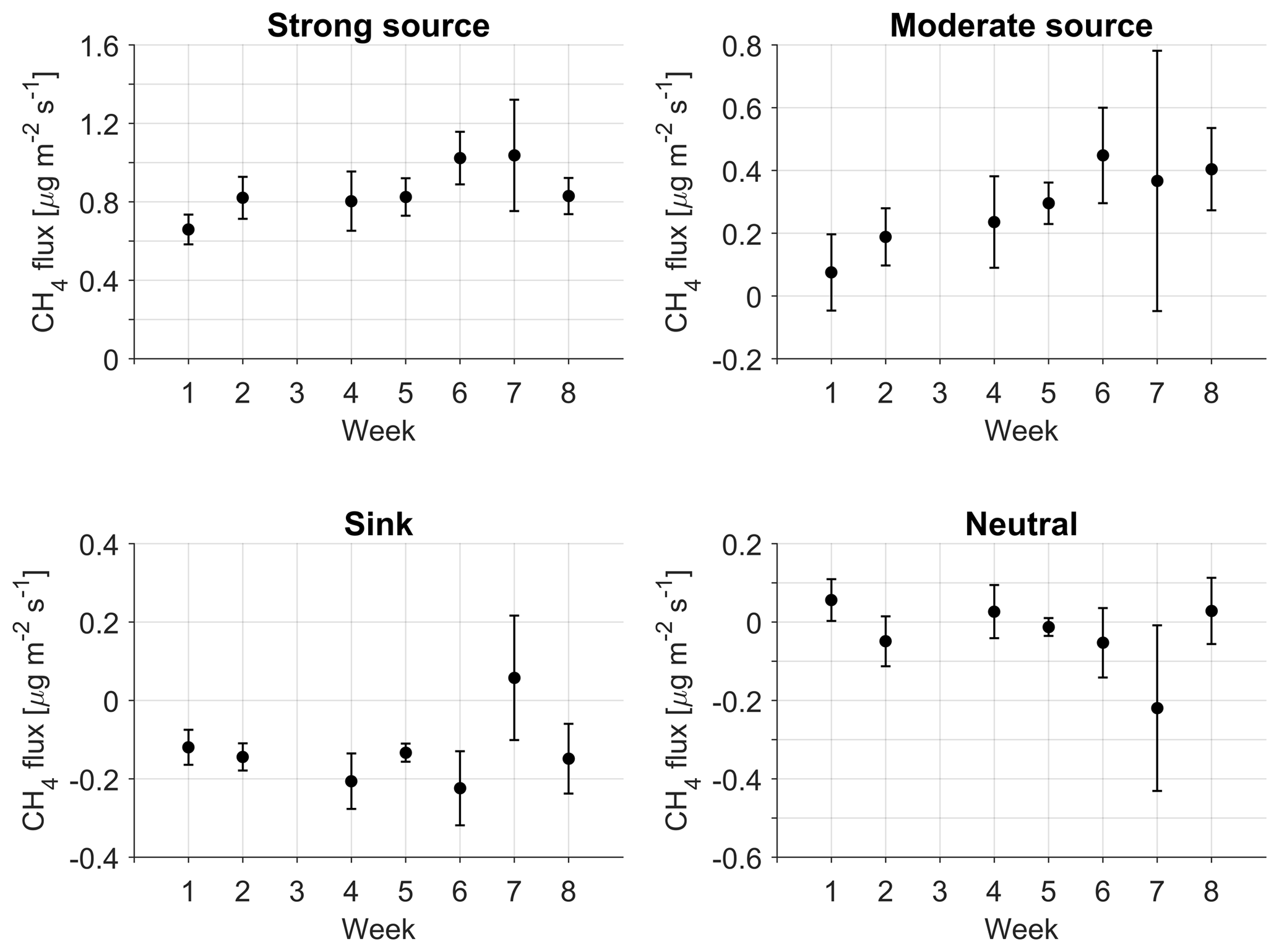
Figure 6Estimates of the LCC group-specific fluxes calculated from weekly data (1 indicates 5–11 July; 2 indicates 12–18 July; 3 indicates 19–25 July, data missing; 4 indicates 26 July–1 August; 5 indicates 2–8 August; 6 indicates 9–15 August; 7 indicates 16–22 August; 8 indicates 23–29 August). The vertical bars indicate the 95 % confidence intervals.

Download

3.3 Upscaled CH₄ fluxes

By upscaling the mean CH₄ fluxes estimated for the LCC groups, we estimated the effect of the EC tower location on the spatial representativeness of the mean CH₄ flux observed during the growing season of 2014 (0.208 $\mathrm{\mu }\mathrm{g}{\mathrm{CH}}_{\mathrm{4}}{\mathrm{m}}^{-\mathrm{2}}{\mathrm{s}}^{-\mathrm{1}}$). In other words, adopting the data shown in Table 5 as a reference for the CH₄ flux averaged over the study area, we could calculate the sensor location bias for CH₄ flux (Fig. 5) similarly to the results shown in Sect. 3.1 for LAI, terrain elevation, TWI and LCC proportions. As the relative area of the coastal waters is significant within the study area but minor in the average flux footprint (Fig. 1, Table 4), these areas were excluded from the upscaling domain.

Calculating the sensor location bias for CH₄ flux is equivalent to a linear transformation of the observed fluxes. Thus, the pronounced directional dependence of CH₄ fluxes translates into an equally pronounced variation in this bias estimate, which ranged approximately from −200 % to 400 % for individual data points and from −170 % to 230 % on average (Fig. 5). The bias was smallest in eastern and western wind directions. However, the effective LCC composition is very different in these directions, with a much smaller coverage of fens in the west (Fig. 3).

The areally averaged CH₄ flux depended on the upscaling domain in a non-monotonous manner (Fig. 7). The uncertainty of the mean measured CH₄ flux (Sect. 2.3.2) was small (0.007 $\mathrm{\mu }\mathrm{g}{\mathrm{CH}}_{\mathrm{4}}{\mathrm{m}}^{-\mathrm{2}}{\mathrm{s}}^{-\mathrm{1}}$) due to a large number of observations and was ignored in Fig. 7b. Defining the reference area as a function of the radius of a circular area centred at the EC tower, the magnitude of sensor location bias was less than 10 % for the distances of 640–1350 m. Acknowledging the statistical uncertainty in the upscaled fluxes, determined from the LCC group-specific uncertainty estimates (Table 5), the measured mean flux was within the 95 % confidence interval for distances larger than approximately 600 m. For the primary study area, the mean bias during the growing season was 13.9 % and the corresponding 95 % confidence interval was [−0.3 %, 32.9 %] (Table 6). While formally the overestimation of EC measurements of the CH₄ flux averaged over the study area was not statistically significant (p>0.05), the estimated sensor location bias would be lower if the study area were originally defined by a radius of 800–1000 m (Fig. 7). Here, we do not suggest that the study area should be defined post hoc but advocate a footprint-based analysis to assess the representativeness of measurements at different spatial scales. Adopting the regional upscaling area of 35.8 km² as the reference results in a sensor bias of 30 % [12 %, 55 %] for the CH₄ flux (Table 6).

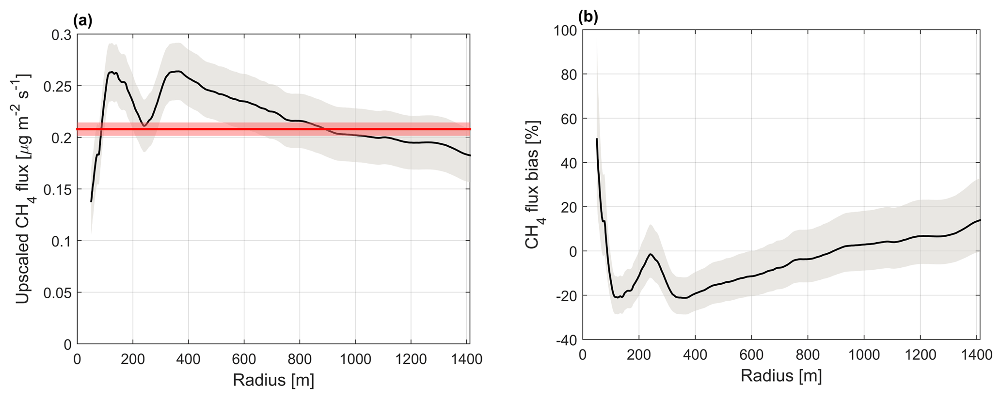
Figure 7Upscaled CH₄ flux within a circular area as a function of the distance from the EC tower (a) and the corresponding sensor location bias according to Eq. (6) (b). The red line indicates the mean measured flux. The shaded areas represent the 95 % confidence intervals.

Download

Table 6Upscaling of CH₄ fluxes ($\mathrm{\mu }\mathrm{g}{\mathrm{CH}}_{\mathrm{4}}{\mathrm{m}}^{-\mathrm{2}}{\mathrm{s}}^{-\mathrm{1}}$) based on the LCC group-specific flux data shown in Table 5.

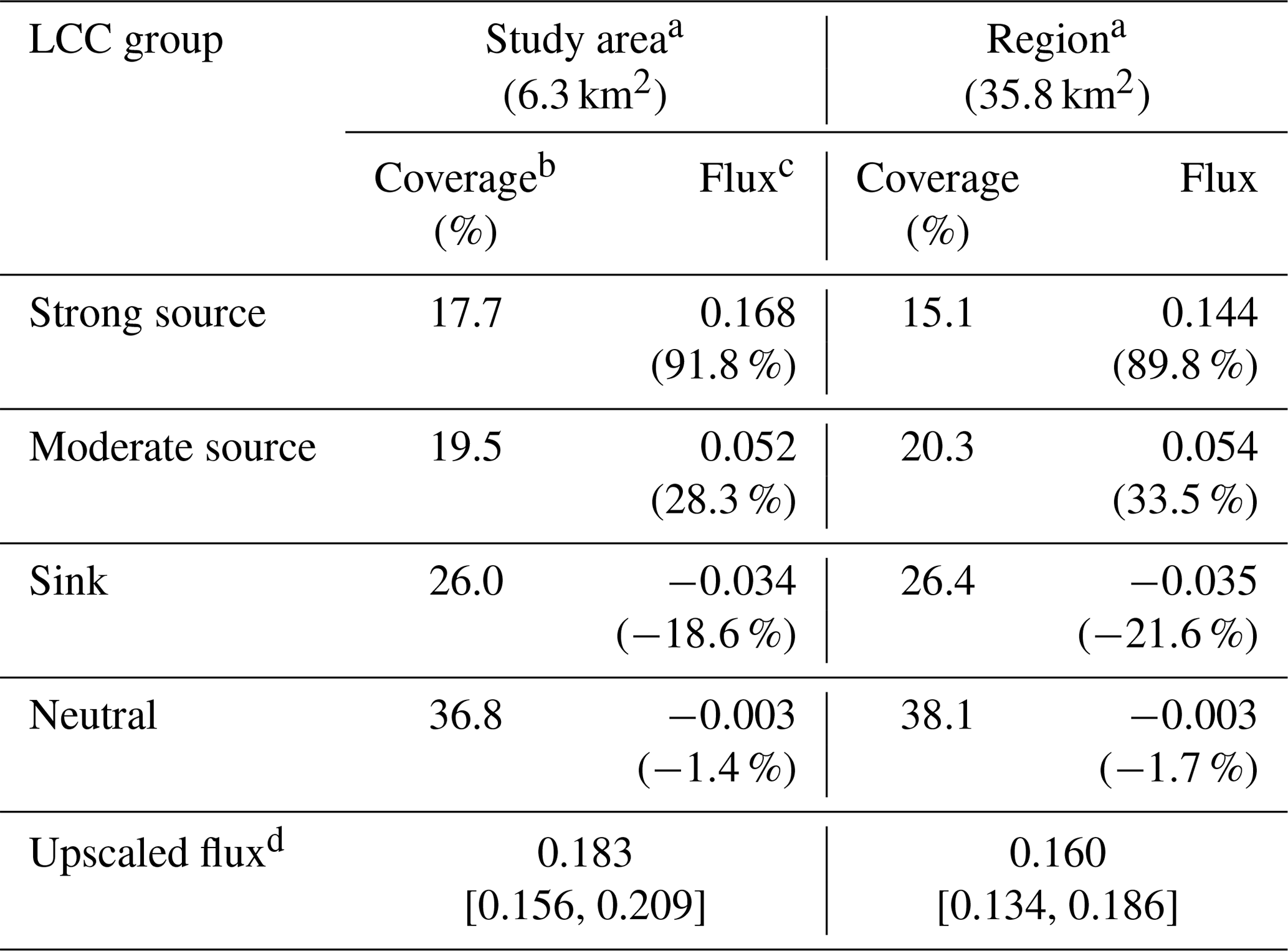
^a “Study area” refers to the circle with a radius of 1.4 km centred at the EC mast. “Region” is shown in Fig. S2. ^b Marine areas are excluded from upscaling. ^c Calculated as LCC group-specific flux multiplied by the relative coverage. The value in parentheses is equivalent to this flux divided by the upscaled flux. ^d The values in square brackets indicate the 95 % confidence interval.

Download Print Version | Download XLSX

Even though the coverage of our nine basic LCCs clearly differed from their footprint-weighted contributions (Table 4), the four LCC groups, aggregated according to the assumed CH₄ emission potential of LCCs, covered areas rather similar to those within the original study domain (Table 6). Within the regional upscaling area of 35.8 km², the strong emitters were less common, but the total flux was only 13 % lower than within the original study area. On the other hand, freshwater bodies occupy a larger relative area (Table 4). These were included here in the “moderate source” LCC group, but the actual emissions from these ecosystems could not be estimated as their total area within the flux footprint is minute. Nevertheless, there is increasing evidence that Arctic lakes and ponds emit significant amounts of CH₄ (Wik et al., 2016). At all scales, it was necessary to allow for the sink areas that play a significant role in the upscaled balance. However, the agreement of CH₄ fluxes between different scales may be considered somewhat fortuitous and implies little about carbon dioxide and other scalar fluxes that have different spatial patterns.

3.4 Methodological issues

Our results obviously depend on the quality of the land cover classification. The LCC accuracy assessment indicates that especially the flood meadow LCC is poorly classified (Mikola et al., 2018); however, this LCC only appears along the brook and has a very limited coverage. More importantly, the dry fen, wet fen and graminoid tundra pixels may be partly mixed up. The field data and multivariate data analysis of Mikola et al. (2018) indicate that the variations in plant functional type composition within these LCCs indeed overlap, which impairs the classification of the “strong source” and “moderate source” LCC groups and effectively precludes modelling that resolves individual LCCs. On the other hand, the large areas of bare ground and lichen tundra with low organic soil content, i.e. the assumed CH₄ sink areas, can be identified reliably (Mikola et al., 2018).

Despite the uncertainties, the land cover classification allowed us to meaningfully group the surface elements according to their CH₄ exchange potential. This relationship shows that the LCC reflects the integrated effect of a range of processes that control net production and efflux of CH₄, such as the availability of substrates and gas transport routes (Davidson et al., 2016, 2017). Thus, a vegetation classification based on VHSR satellite imagery provided us with a straightforward means of upscaling the average LCC group-specific fluxes. As the predominant part of CH₄ flux variance resulted from the varying contributions of different LCCs, we did not consider additional environmental controls. Such simplicity is welcome since statistically robust EC-based flux estimates for scales exceeding the flux footprint would require spatial replication with multiple EC towers (Hill et al., 2017). Our approach serves as an alternative to a common method of deriving LCC-specific data from (a typically more limited set of) flux chamber measurements and upscaling these either directly (e.g. Schneider et al., 2009; Davidson et al., 2017) or by first modelling their temporal variation (e.g. Marushchak et al., 2016). Matthes et al. (2014) showed that more nuanced insights into the spatial drivers can be achieved by the use of multiple EC towers and periodic remote sensing images and by examination of both the abundance and spatial fractal structure of vegetation.

Even though the KM model constitutes an appropriate tool for describing turbulent transport over an aerodynamically smooth surface such as tundra, any footprint estimate involves both structural and input-related modelling uncertainties. The KM model has been tested by Kljun et al. (2003), Marcolla and Cescatti (2005), Neftel et al. (2008) and Arriga et al. (2017) against experimental data and more complex footprint models. All these studies conclude that the KM model performs well, but we note here that there may be a tendency for too-smooth footprint distributions in the along-wind direction. As pointed out in Sect. 2.3.2, we did not try to explicitly estimate the errors related to the flux footprints but assumed that the confidence intervals determined for the LCC group-specific fluxes reflect the overall uncertainty contained in any data employed in the statistical model. Because of this approach, the uncertainty of the results shown in Figs. 3 and 4 could not be quantified. Overestimation of footprint distribution in larger distances would mean that the contribution of graminoid tundra might be slightly underestimated and that of shrub tundra overestimated as the proportions of these LCCs have a rather systematic dependency on the distance from the EC mast. If the overall LCC heterogeneity of a site became more apparent when viewing it as a function of distance rather than direction, our statistical method would be more dependent on the footprint model and the results would probably be more uncertain.

We obtained statistically significant estimates for the LCC group-specific fluxes when employing the whole data set of 8 weeks, but the performance of the model was observed to deteriorate as the number of data was reduced. This can be observed from the weekly results (Fig. 6), in which the confidence intervals are temporally varying and larger than those for the whole data set; in some cases, the results were not consistent with the original flux hypotheses (at the chosen significance level). As wind direction is the primary control of the flux footprint, and consequently the LCC proportions associated with EC measurements (Fig. 3), it is necessary that the variation in wind directions during each period sufficiently covers all the relevant LCCs. This obviously depends on the degree and nature of LCC heterogeneity at the site in question. In our weekly results for Tiksi, the directional coverage was clearly incomplete during 16–22 August 2014, when there were few observations for the sector extending from the north-west to the south-east, leading to uncertain flux estimates for that particular period (Fig. 6). Nevertheless, the LCC group-specific fluxes estimated on a weekly basis improved the overall model performance during the whole study period (R²=0.836, RMSE of 0.0894 $\mathrm{\mu }\mathrm{g}{\mathrm{CH}}_{\mathrm{4}}{\mathrm{m}}^{-\mathrm{2}}{\mathrm{s}}^{-\mathrm{1}}$, MAE of 0.0619 $\mathrm{\mu }\mathrm{g}{\mathrm{CH}}_{\mathrm{4}}{\mathrm{m}}^{-\mathrm{2}}{\mathrm{s}}^{-\mathrm{1}}$).

While the weekly results indicated that there is temporal variation in the LCC group-specific fluxes, the longer-term upscaling was rather insensitive to temporal resolution of these data. The weekly values produced an upscaled flux of 0.162±0.063 $\mathrm{\mu }\mathrm{g}{\mathrm{CH}}_{\mathrm{4}}{\mathrm{m}}^{-\mathrm{2}}{\mathrm{s}}^{-\mathrm{1}}$ for the original study area, i.e. only slightly lower (by 11 %) but a much more uncertain estimate than the one obtained for the whole data set (Table 6).

We suggest that estimation of LCC-specific fluxes, accomplished here with a regression model, provides a new avenue to filling the inevitable gaps in the measurement data time series. This proposition is supported by the good out-of-sample validation statistics obtained (Sect. 3.2), as holding the validation data out during parameter estimation is equivalent to generating missing data that need to be gap-filled. This kind of an approach is potentially applicable to those data gaps that are related to the gas concentration measurement, for example due to malfunctioning of the gas analyser, i.e. gaps that appear in the CH₄ flux data but not in the momentum and sensible heat fluxes.

Another methodological implication of our results concerns the definition of a study area. It is customary to report a “site description” that documents the key ecological characteristics of the area of interest. Within a homogeneous environment, collating the necessary site data is straightforward in terms of statistical representativeness because the outcome is insensitive to the spatial sampling design. Furthermore, the representativeness of EC measurements can be simply assessed by considering the coverage of a single target LCC within the flux footprints. In heterogeneous environments, however, there is a risk for a serious mismatch between the EC flux measurements and the site data, even in cases of an unbiased description of the study area. Our results show that the land cover type composition sampled by the EC measurement was significantly different from the actual LCC coverage within our study area, which as such was originally chosen to be consistent with the dimensions of a typical flux footprint and considered characteristic of the landscape.