the Creative Commons Attribution 4.0 License.
the Creative Commons Attribution 4.0 License.
 | 13 May 2019
Modeling soil organic carbon dynamics in temperate forests with Yasso07
Delphine Derrien
Markus Didion
Jari Liski
Thomas Eglin
Manuel Nicolas
Mathieu Jonard
Laurent Saint-André
In a context of global changes, modeling and predicting the dynamics of soil carbon stocks (CSs) in forest ecosystems are vital but challenging. Yasso07 is considered to be one of the most promising models for such a purpose. We examine the accuracy of its prediction of soil carbon dynamics over the whole French metropolitan territory at a decennial timescale.
We used data from 101 sites in the RENECOFOR network, which encompasses most of the French temperate forests. These data include (i) the quantity of above-ground litterfall from 1994 to 2008, measured yearly, and (ii) the soil CSs measured twice at an interval of approximately 15 years (once in the early 1990s and around 2010). We used Yasso07 to simulate the annual changes in carbon stocks (ACCs; in tC ha−1 yr−1) for each site and then compared the estimates with actual recorded data. We carried out meta-analyses to reveal the variability in litter biochemistry in different tree organs for conifers and broadleaves. We also performed sensitivity analyses to explore Yasso07's sensitivity to annual litter inputs and model initialization settings.
At the national level, the simulated ACCs ( tC ha−1 yr−1, mean ± SE) were of the same order of magnitude as the observed ones ( tC ha−1 yr−1). However, the correlation between predicted and measured ACCs remained weak (R2<0.1). There was significant overestimation for broadleaved stands and underestimation for coniferous sites. Sensitivity analyses showed that the final estimated CS was strongly affected by settings in the model initialization, including litter and soil carbon quantity and quality and also by simulation length. Carbon quality set with the partial steady-state assumption gave a better fit than the model with the complete steady-state assumption.
With Yasso07 as the support model, we showed that there is currently a bottleneck in soil carbon modeling and prediction due to a lack of knowledge or data on soil carbon quality and fine-root quantity in the litter.
- Article
(4788 KB) -
Supplement
(2933 KB) - BibTeX
- EndNote


The current global carbon stock (CS) in soils, including forest litter and peatlands, is 1500 to 2400 GtC and thus greatly exceeds stocks in vegetation, found mainly in forests (350 to 550 GtC) and in the atmosphere (829 GtC in 2011; IPCC, 2014). Soils share a common interface with all the other spheres and play a key role in driving the global carbon cycle. Soil CS dynamics are directly related to the greenhouse gas emissions (notably carbon dioxide; CO2) that are leading to the global warming effect (IPCC, 2014). An accurate estimation of soil CS dynamics would allow us to better understand the turnover rate and fate of soil carbon flux at both local and global geographical scales. In the context of global changes, accurate estimation is essential in evaluating the climate change mitigation potential of forests and supporting environmental policy decisions.
Significant challenges exist when attempting to accurately estimate changes in soil CSs. Current soil monitoring networks are generally not able to detect changes on timescales of less than 10 years (Saby et al., 2008). To obtain estimates for changes in soil CSs at shorter intervals, as is, for example, required for annual reporting to the United Nations Framework Convention on Climate Change and the Kyoto Protocol, using models is encouraged (IPCC, 2011). Numerous models have been elaborated to evaluate soil carbon dynamics (Manzoni and Porporato, 2009). The vast majority of terrestrial soil carbon models developed at the global or the plot scale (e.g., CENTURY in Parton et al., 1987; RothC in Coleman and Jenkinson, 1996; and ORCHIDEE in Krinner et al., 2005) assume that decomposition is the first-order decaying process, which accounts for the size of soil carbon pools. However, the assumption has been criticized, and it has been argued that a priming effect and the associated carbon pool interactions should also be considered in model algorithms (Wutzler and Reichstein, 2013). The dynamics of carbon pools depend on the quantity and quality of litter inputs and on temperature, soil moisture and other soil parameters, e.g., texture, structure, chemical richness, pH, etc. (Todd-Brown et al., 2012). Incorporating explicit mechanisms such as microbial activities or carbon protection by the soil matrix into soil carbon models has repeatedly been suggested in recent years (Schmidt et al., 2011; Lehmann and Kleber, 2015). However, for forest ecosystems, refined mechanistic input data often remain limited. Accordingly, the typical time step for litter input demanded by most forest soil carbon models is yearly, rather than monthly (but see RothC, Coleman and Jenkinson, 1996) or daily (but see Romul in Chertov et al., 2001; Didion et al., 2016). At this yearly timescale, it is common to consider microbial communities and processes to be relatively stable factors (Todd-Brown et al., 2012); in this case, the assumption that carbon dynamics are governed by first-order decay may therefore be reasonable.
This is the choice made by the group who built the Yasso (Liski et al., 2005) and Yasso07 (Tuomi et al., 2009, 2011a, b) models. Yasso07 is an improved version of Yasso with more refined carbon pooling and abundant data for calibration. The model developers' intention was to make their models suitable for general forestry applications by taking into account the limited availability of forest soil and litter data (Liski et al., 2005). Yasso07 explicitly defines several pools of chemical compounds in litter carbon (Tuomi et al., 2011b) and possesses well defined, biologically meaningful and measurable parameters. Thanks to these qualities, Yasso or Yasso07 has been applied in more than 150 case studies (https://en.ilmatieteenlaitos.fi/yasso-publications, last access: 21 April 2019) in forest ecosystems in the Northern Hemisphere, with generally high satisfaction levels when compared with measured carbon values (e.g., Karhu et al., 2011; Rantakari et al., 2012; Ortiz et al., 2013; Didion et al., 2014; Lu et al., 2015; Wu et al., 2015). Yet so far most of these applications have been limited to local case studies, especially in cold forests with limited tree species diversity (e.g., boreal or montane forests). Rarely have previous studies validated Yasso07 based on data (i) from long-term observations (here defined as >10 years), (ii) from temperate forests with a much higher diversity of tree species or (iii) on changes in CSs (in tC ha−1 yr−1). This is partially due to the lack of extensive long-term soil carbon monitoring in forest ecosystems, which differs in climatic and soil conditions and species and stretches over large territorial scales. Nevertheless, Yasso07 is considered to be one of the potentially appropriate models for evaluating national and continental inventories of the forest carbon balance in Europe (Hernández et al., 2017). It is therefore of considerable interest to assess the ability of Yasso07 to reflect the carbon balance in different European forest ecosystems at large spatio-temporal scales. Moreover, as a carbon-pool-based model, Yasso07 shares certain principles with other prevailing soil carbon models in the same genre (e.g., RothC, CENTURY, etc.). Applying Yasso07 as an example model in this case study may also allow us to improve future carbon modeling for temperate forests in general.
The recorded field data for CSs and litter quantity dynamics from the RENECOFOR network (http://www.onf.fr/renecofor/@@index.html, last access: 21 April 2019), National Forests Office (ONF), France, offered us a valuable opportunity for model validation. The 101 forest sites included in this study are located all over the French metropolitan territory and cover the most common forest types and tree species. For each site, annual measurements of litterfall were available in addition to two inventories of soil organic CSs with an average interval of 15 years (minimum of 12 years and maximum of 20 years). These data allowed us to use site-specific observed soil CSs and above-ground litterfall dynamics as model input data. Approximations in model input data have been identified as a major source of uncertainty for estimates in models for changes in soil CSs (Ortiz et al., 2013). By ensuring solid input data, we were able to minimize this source of uncertainty and focus on the inherent model structure.
We hope to contribute to the further development of soil carbon modeling by (i) testing and characterizing the ability of Yasso07 to model soil CS dynamics for temperate forests, (ii) identifying limitations and providing suggestions for a better adaptation of the model for C dynamics in both deciduous and evergreen temperate forests, and (iii) discussing the perspectives based on the current state of the art in soil carbon modeling. Associated with the above aims, our null hypotheses are as follows: (i) Yasso07 predicts accurate and unbiased CS changes at the national scale, and (ii) the model's fit residuals (predicted data minus observed data) have null relationships with site characteristics (e.g., location, climate, forest type, soil type and initial CS).
2.1 The Yasso07 model
The Yasso07 dynamic soil carbon model is based on the general assumption that the soil CS is driven by the decomposition of different litter types, which may differ in quantity and quality and by climatic conditions. Litter carbon quality is represented by four chemical compound groups with different decomposition rates (Tuomi et al., 2009). Soil organic carbon is divided into these four relatively labile carbon pools and one recalcitrant pool called “humus” (H) (Fig. S1 in the Supplement). The five pools differ in specific mass loss rates and mass flows. As in many other pool-based models, the H pool is considered to be the oldest and most stable carbon pool, although recent studies have thrown doubt on its stability and even its physical existence (see Lehmann and Kleber, 2015). Some mass flows correspond to CO2 release (microbial respiration). The mean residence time of carbon in these pools varies, lasting several months (i.e., water soluble compounds – W), a few years (i.e., acid-hydrolyzable compounds – A; non-polar solvent, ethanol or dichloromethane compounds – E), several decades (i.e., non-soluble and non-hydrolyzable compounds – N) or even several centuries (i.e., H).
Mathematically, the kernel equation of Yasso07 can be written as follows:
where symbols in bold capital letters denote either vectors or matrices, while those in small letters in parentheses denote scalars, X(t) is the vector describing the masses of the five carbon pools (A, W, E, N and H) at time t, is the vector describing carbon mass changes in soil at time t, Ap is the mass flow matrix describing carbon allocation among pools, K(c) is the decomposition matrix describing the decomposition rates as a function of climatic conditions (c), and I(t) is litter input to the soil and is equal to 0 for the last pool, since “H” does not exist in litter form (Eq. 1a) and can be expressed in a more detailed form. This form is
where pF→T is the relative mass flow parameter between two pools (from F to T; F and T can be any two pools among A, W, E, N and H) in the soil (dimensionless, [0, 1]).
Temperature and precipitation are assumed not to affect mass flow p but do influence mass loss rate ki (i= A, W, E, N or H) according to the following:
where αi is the mass loss rate parameter of the chemical pool i; and β1, β2 and γ are parameters related to temperature (T; in ∘C) and precipitation (Pa; in mm).
To take into account the effect of litter size on the litter decomposition rate, ki was multiplied by a litter size factor (hs), which makes it possible to distinguish between different types of litter (e.g., foliage, coarse woody debris, stems, etc.), differing in diameter (d; in mm):
where φ1, φ1 and r are parameters related to litter size.
Yasso07 has 44 parameters calibrated according to the Markov chain Monte Carlo (MCMC) method with the Metropolis–Hastings algorithm (Tuomi et al., 2011a). Currently, several calibrated parameter sets for Yasso07 are available, including the two most recent sets published by Tuomi et al. (2011) and Rantakari et al. (2012). Compared with the Rantakari (2012) set, the Tuomi (2011) set was calibrated using a wider range of observed foliage and root decomposition data. It is based on a combination of three sources of data: (i) a global dataset (n>9000) of litterbags for mass loss of non-woody litter from approximately 100 sites in Europe and North and Central America covering a wide range of climate and soil conditions, forest types and tree species; (ii) a dataset (n>2000) for mass loss of decomposing woody litter measured in northern Europe; and (iii) measured accumulation rates of soil carbon pools in forest sites along a 5300-year soil chronosequence in southern Finland to determine the residence time of the H carbon pool. The Tuomi (2011) parameter set contains 10 000 parameter vectors (each vector contains the values of all 44 Yasso07 parameters), which are randomly generated to take into account the stochastic effect. In this study, we adapted the Tuomi (2011) set to the RENECOFOR dataset.
2.2 RENECOFOR network
The RENECOFOR network is part of the Level II network of the International Co-operative Programme on Assessment and Monitoring of Air Pollution Effects on Forests (ICP Forests). The 101 sites (Fig. 1) considered in this study cover the most common types of forest ecosystems in France, including evenly aged forests in plains, pine plantations and unevenly aged mountain forests. They also host most of the tree species in France and central Europe, including Quercus robur, Quercus petraea, Pseudotsuga Menziesii, Picea abies, Fagus sylvatica, Pinus pinaster, Pinus sylvestris and Abies alba. At each forest site, annual woody and non-woody litter quantities are either directly measured or estimated based on existing dendrometric data.
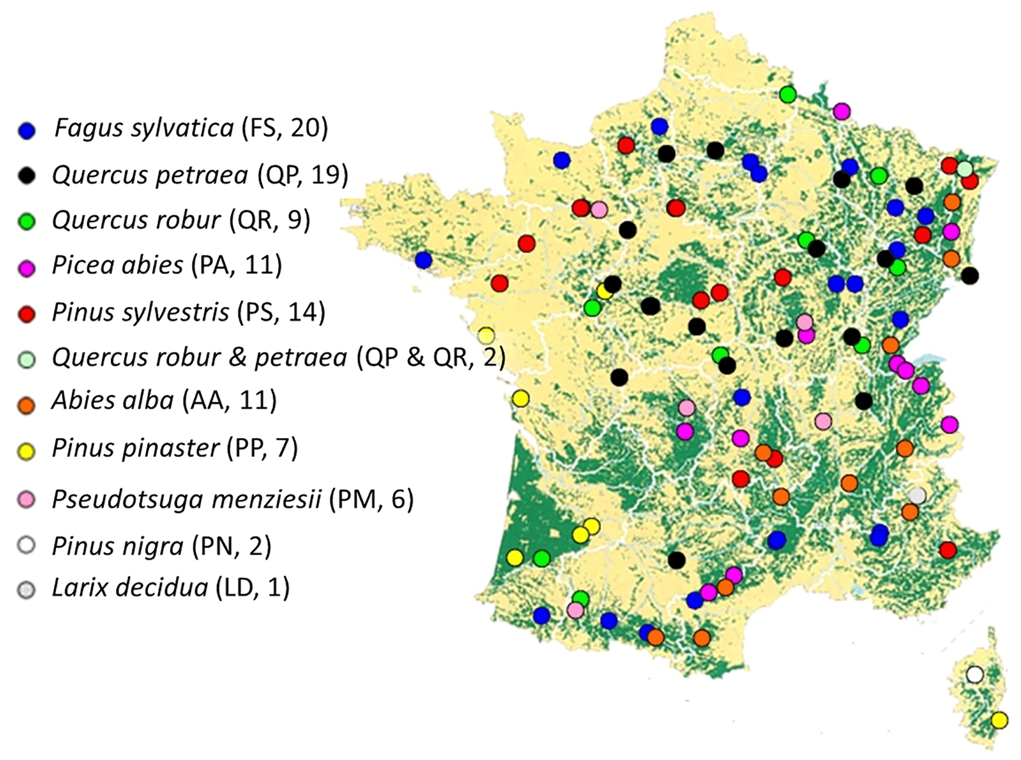
Figure 1Geographical distribution of the sites in the RENECOFOR network used to test Yasso07 performance (see also Jonard et al., 2017). Forested areas are represented in green. Each circle represents one site; the color represents the dominant tree species on the plot. The species abbreviation and number of sites per species are indicated in parentheses. One site (Picea abies 39b) was not used due to data incompletion.
2.2.1 Soil carbon and soil physical and chemical properties
At each site, soil CSs were measured twice at an interval of approximately 15 years (1993–1995 for the first assessment and 2007–2012 for the second one). At each site and for each assessment, soils were sampled to a depth of 0.4 m at five points selected in each of five subplots, and the samples were divided into different layers (0–0.1, 0.1–0.2 and 0.2–0.4 m), including both organic and mineral soil layers. The temporal changes in soil CSs to a depth of 0.4 m were analyzed by Jonard et al. (2017). Composite samples were produced for each layer and subplot then analyzed for mass, bulk density, soil organic carbon, and physical and chemical properties, including texture (proportion of clay, silt and sand; in %); pH value; total nitrogen stock (in t ha−1), the carbon : nitrogen ratio (dimensionless); total phosphorus stock (in t ha−1); and stocks of exchangeable aluminum (Al), calcium (Ca), potassium (K) and magnesium (Mg; in kmol ha−1). We used the soil physical and chemical property data measured during the first assessment (1993–1995) for residual analyses (see Sect. 2.7)
Regarding the CSs from 0.4–1.0 m in depth, only data from the first assessment (1993–1995) were available. Soil samples were obtained from only one soil profile per site at two mineral layers (0.4–0.8 and 0.8–1.0 m). Bulk density and carbon concentrations measured at these layers were used to estimate soil CSs to a depth of 1.0 m. Table 2 summarizes the data source for each of the 101 sites in the RENECOFOR network (http://www.onf.fr/renecofor/sommaire/renecofor/reseau/20090119-130815-828957/@@index.html, last access: 21 April 2019). More detailed information about each site and the soil sampling procedure is available in Supplement I (Table S1) and Jonard et al. (2017).
2.2.2 Climate data
The climate data required by Yasso07 include annual mean precipitation (mm) and annual maximum, mean and minimum temperatures (∘C). These measured data were obtained from the national Météo-France meteorological stations (http://www.meteofrance.com, last access: 21 April 2019) nearest to each RENECOFOR site.
2.3 Litter quantity
Litter input (in tC ha−1 yr−1) comes from several sources (see Table 2). We assumed a 0.5 conversion factor between biomass (dry matter) and carbon (Thomas and Martin, 2012).
Above-ground litter input from living trees includes leaves for broadleaves and needles for conifers, small branches, fruits and miscellaneous items (e.g., flowers, buds, etc.). Above-ground litterfall mass was measured annually between 1994 and 2008. For sites where litter quantity data from 1992–1993 and 2009–2012 were lacking, we used the mean litter quantity of all the other years at the same site. The observed branch size in this above-ground category was less than 2 cm (fine branches). Branches and stems bigger than 2 cm due to natural mortality were rare (since they can be salvaged) and were therefore not included in our calculations.
Coarse woody litter input from harvesting residue or storms were estimated from full inventories performed by the ONF since 1991. Missing years of litter input for this category were gap-filled with the average over the period. On average, 3 years are missing per site, though there are considerable differences amongst sites. The mode was 1 year, and six sites had 10–11 missing years. We assumed that the residues due to harvesting or storms would be coarse branches (> 4 cm in diameter, confirmed with the ONF) based on above-ground tree characteristics. The quantities were estimated on the basis of repeated stand inventory data and species-specific height–girth relationships and biomass. Litter input from stems was set to 0, since in most cases, stem wood was removed from the site after storm damage. Litter input from coarse woody roots was considered to be equal to total root biomass, which was estimated through meta-analysis-based allometric equations proposed by Cairns et al. (1997). More detailed information about forest inventories and storm events occurring at each site is available in Supplement I (Table S1).
Litter input from fine roots (here defined as roots of ≤5 mm in diameter), especially the finest ones with a diameter ≤2 mm, can significantly contribute to carbon sequestration in soils (Brunner et al., 2013; Kögel-Knabner et al., 2002; Berg and McClaugherty, 2008). Fine root litter was assumed to be proportional to that of foliage, which was measured in the RENECOFOR sites (see the following paragraph). Jonard et al. (2017) suggested using the generic equation published by Raich and Nadelhoffer (1989) and, simultaneously, adopted the hypothesis that fine-root litter production represents about one-third of the carbon allocated to roots (Raich and Nadelhoffer, 1989):
where Ifine root and Ifoliage are the litter input of fine roots and foliage, respectively (in tC ha−1 yr−1).
The relationship between fine-root and foliage litter inputs can be highly variable depending on tree species, stand characteristics and climate, and the generic equation may not reliably represent such variability. To counter this, we carried out a sensitivity analysis to investigate the response of the model fit to the choice of fine-root-to-foliage ratio varying from 0.1 to 4.0 (see Sects. 2.6 and 3.2). Yet, when applying the equation of Raich and Nadelhoffer (1989; Eq. 4) over all the RENECOFOR sites, we found that fine-root-to-foliage ratios had a median of 1.0 and a mean of 1.0–1.1 for both coniferous and broadleaved sites (Fig. S2). Hence, we chose to use the 1.0 ratio over all the RENECOFOR sites to present the outcomes of the model fit and residual analyses from the simulations (see Sect. 3.3). This facilitated our evaluation of site factors (e.g., dominant tree functional type, climatic and soil features) without adding a source of variability introduced by fine-root-to-foliage ratio.
2.4 Litter carbon quality
In the RENECOFOR network, there are no measured data for litter carbon quality, defined as the relative amount of litter carbon belonging to four different carbon pools (A, W, E and N). Therefore, we carried out a meta-analysis of the data collected in the literature where authors used chemical fractioning procedures or near-infrared spectroscopy (NIRS) techniques to measure litter carbon quality. The data were restricted to non-tropical areas. Chemical data on litter composed of coarse tree organs (e.g., stems, coarse branches) are relatively scarce, so we used the tree stem wood data compiled in Pettersen (1984), Rowell et al. (2005) and Rowell (2012). These three studies cover a wide range of temperate tree species from North America, Japan and Russia. Data on foliage and root litter carbon quality were taken either from networks such as CIDET (Trofymow, 1998) and LIDET (http://andrewsforest.oregonstate.edu/research/intersite/lidet.htm, last access: 21 April 2019) or from independent studies in the Northern Hemisphere. The database we used for our meta-analysis is available in Supplement II. The root diameter or branching order can play a significant role in modifying the composition of soil chemical compounds (Fahay et al., 1988; Tingey et al., 2003; Guo et al., 2004). All the measurements included in our meta-analysis on roots refer to fine roots (diameter ≤5.0 mm), although in several studies, e.g., Aber et al. (1990), Aulen et al. (2011) and Stump and Binkley (1993), root size was not clearly indicated. Yet we still included the data from the latter studies, as data are less abundant for roots than foliage. The coarse-root data in the literature were too few for a meaningful meta-analysis; we therefore used stem wood values instead.
We then used the resulting litter carbon quality database to describe the quality of litter input at each site in our study. We portioned the litter input into biochemical classes in the following order of priority: (i) values for the target species, when available in the database; (ii) mean values of the species from the same genus, if data for the target species were absent; and (iii) mean values of the species from the same tree functional type (conifers versus broadleaves), if no data were available at either species or genus level for the target species (see Table 1).
Table 1Litter carbon quality of the species present in the French RENCOFOR network, estimated based on the literature. In the column “Case,” each number corresponds to one case of data availability in the literature: 1 – at least one dataset of complete chemical composition (i.e., for AWEN) exists at species level; 2 – at least one dataset of incomplete chemical composition (only for A, N and the sum of W and E) exists at species level, and in this case, the mean proportion of W and E at genus level is used; 3 – no data are available at species level, but at least one complete dataset of chemical composition exists at genus level; 4 – no data are available at species level, but at least one incomplete dataset of chemical composition exists at genus level, and in this case, the mean proportion of W and E at tree functional type level is used; 5 – no data are available at either species or genus level, and in this case, the mean AWEN composition at tree functional type level is used. Cases 1 to 5 are in descending order of priority. Note: A – acid-hydrolyzable compounds; W – water soluble compounds; E – non-polar solvent, ethanol or dichloromethane compounds; NA – not available.

Table 2A summary of the data used for Yasso07 simulations in the present study. In the “year” columns, the following abbreviations are used: M – measured data; E – estimated data based on measured data; and 0 – noted, but the contribution to litter is negligible. For soil CS measurements, zones in dashed line denote the inventory duration. For each year, each symbol (M and E) only accounts for the general case, hence it is possible that measurements were occasionally omitted at some sites. * Litter input caused by harvest or storms were included (after they had occurred), SD is standard deviation, and litter input is dry matter. Diameters used for defining each litter type are the following: ≤2 cm for fine branches, > 4 cm for coarse woody branches, > 5 mm for coarse woody roots and ≤5 mm for fine roots.

2.5 Initialization of soil carbon quantity and quality
To initialize Yasso07, both the quantity and the quality of the soil carbon are required. Here, the initial CSs were fixed as the soil CSs measured during the first RENECOFOR soil carbon assessment (i.e., model input). Measurement uncertainties of the soil CSs were not considered to be a source of the stochastic effect when Yasso07 was fed, as we were more interested in the output uncertainties related to the model per se (i.e., the choice of the model's parameter set) and in carbon quality settings in the model initialization (see below).
Soil carbon quality, defined as the relative amount of soil carbon in pools A, W, E, N and H in relation to their sum, can be initialized in two ways: with a complete steady-state assumption or with a partial, or transient, steady-state assumption. The classical approach is based on the assumption that carbon quality at the initial state is identical to that at the complete steady state, which can be calculated with the analytical matrix inversion approach based on Eq. (1a). For steady-state CSs (t=ts), carbon gain is equal to carbon loss. Setting , (Eq. 1a) becomes
Solving (Eq. 5), we obtain a steady-state CS at time ts, noted as X(ts):
where I(ts) is a constant vector.
The estimated carbon quality of the steady-state CS X(ts) to the depth of 1.0 m (also noted as CSsteady-state; in tC ha−1) was then applied to the observed CSs to split it into various carbon pools.
The complete steady-state assumption is commonly used in the literature despite considerable controversy, since the assumption does not take the difference in stabilization among the various pools into account (Elliot et al., 1996; Foereid et al., 2012). Soil carbon pools (especially those at sites that have undergone disturbances in recent centuries) may not have achieved a complete steady state but may still be in a transient or partial steady state. In such states, the slow-cycling pools can still be accumulating carbon, while the relatively rapid-cycling pools have already recovered a dynamic equilibrium (Wutzler and Reichstein, 2007). In this study, we equally adopted the partial steady-state assumption to mimic such a circumstance. More precisely, we assumed that the rapid-cycling pools such as A, W and E were at steady state at the first soil survey, while the slow-cycling N and H pools might not yet have reached the steady state. Accordingly, we directly considered the steady-state CS obtained from matrix inversion for A, W and E, but we revised amounts for the N and H pools by calculating the difference between estimated and observed CSs to a depth of 1.0 m. In most cases, the sum of steady-state A, W, E and N was lower than the observed CS; the revised H was then equal to the difference between the latter and the former. Very occasionally, the sum of steady-state A, W, E and N could be greater than the observed CS; the revised N was then calculated as the difference between the sum of steady-state A, W and E and the observed CSs and pool H was forced to zero. The new carbon quality, corresponding to the proportions among the steady-state A, W and E pools and the revised N and H pools, was used to split the observed CS into five pools in real simulations.
2.6 Sensitivity analyses on the impact of initial soil and litter settings on model output
It is important to gain a general idea of the magnitude of the impact on model output and fit of our choices for initial soil and litter settings in the process of model initialization. To this end, we carried out a sensitivity analysis to assess how assumptions on carbon quality (complete steady state versus partial steady state) and carbon quantity as a function of soil depth (observed CSs to a depth of 1.0 m versus observed CSs to 0.4 m) and of fine-root-to-foliage ratios (from 0.1 to 4.0) affected model predictions. Model fit is expressed via the comparison between simulated and observed annual changes in carbon stocks (ACCs) in the soil.
In addition, we conducted another sensitivity analysis to fully explore the effects of all the theoretically possible initial soil carbon quality distributions and that of simulated duration on model outputs. We created a virtual site where climatic conditions and litter input were constant and equal to the average values of all the RENECOFOR sites. By fixing its initial soil CS to 100 tC ha−1, we permuted the initial percentage of the soil carbon pools, with minimum and maximum percentages fixed at 5 % and 80 %, respectively. We used four levels of simulated duration (1, 10, 100, 1000 and 10 000 years) for each combination of soil carbon quality distribution. Based on averaged soil and litter carbon data from the RENECOFOR sites, the simulations were carried out for both broadleaved and coniferous forest types. Here, we present only the results for the virtual broadleaved stands, as the results between conifers and broadleaves did not change much, especially over the long term.
2.7 Running Yasso07 and statistical analyses
We used the same FORTRAN code as Yasso07 version 1.0.1 in Didion et al. (2014) for all the model simulations. For each type of analysis (both RENECOFOR site-specific and sensitivity analyses), we conducted 10 simulations. In each simulation, one parameter vector was randomly chosen from the 10 000 parameter vectors.
For each site, we calculated ACC (in tC ha−1 yr−1), i.e., the difference in CSs between the two national RENECOFOR assessments standardized by the temporal interval (t2−t1), as follows:
where, CS, CS and CS are, respectively, the simulated CS to a depth of 1.0 m at year t2 and the observed CS at years t2 and t1, which are around 1994 and 2010, depending on the site.
To compute ACCsim (Eq. 7), some previous studies used a simulated CS at the starting year instead of an observed one (e.g., Ortiz et al., 2013). In such a case, it is of primary importance to judge a “steady-state year” prior to the starting year for which observed data are available. From the estimated steady-state year, a spin-up or real model simulation is then followed to obtain a simulated CS at the starting year. In our simulations, the observed soil CS at t1 served as the model input to set initial soil quantity and to calculate ACC (Eq. 7). This allows avoiding such a judgement on steady-state year, which can be sometimes subjective. This allowed us to better focus on the effect of initialized soil carbon quality, for which we calculated both complete and partial steady-state assumptions (see Sect. 2.5).
Two reasons support our choice to compare ACCsim with ACCobs instead of comparing CS with CS. First, the parameter sets of Yasso07 were calibrated for a soil depth of 1.0 m, while CS data from the two RENECOFOR assessments were only available to 0.4 m (because no data from 0.4–1.0 m in depth were available from the second assessment). It is therefore reasonable to assume that the observed CS data are not comparable with Yasso07 estimates. However, focusing on carbon changes instead of CSs may largely erase this bias. Indeed, previous studies have evidenced that carbon dynamics are much less active at deep soil layers than at superficial layers (Jandl et al., 2014; Balesdent et al., 2018). Second, ACC indicates if a site is gaining or losing soil carbon and whether this information is sometimes more important than the site's CS value. Using a metric standardized by the year, such as ACC, can also facilitate comparing results in future studies. One exception was for our sensitivity analysis on the effect of initial soil carbon quality (Sect. 2.6), where we chose CS instead of ACCsim, since the initial soil CS was fixed at 100 tC ha−1. Despite our primary focus on ACC, we also compared the simulated steady-state CS (CSsteady-state, in tC ha−1) obtained from the initialization procedure (see Sect. 2.5) with the CS down to 1 m in depth; this was to check if Yasso07 was able to predict stocks to 1.0 m depth that indeed reached the level of observed stocks (see Fig. S4).
To test the performance of Yasso07 in estimating changes in soil carbon at the RENECOFOR sites, we used an analysis of variance (ANOVA) to analyze the residuals of the changes in carbon, here defined as the difference between the simulated and observed values. The following environmental and biological factors were tested: site geographical location (latitude, longitude and altitude), the climatic condition (temperature and precipitation), soil type, tree functional type and tree species. Before each ANOVA, we tested the normality of the data with a Shapiro–Wilk test. For the sensitivity analyses, we performed loess regressions (Fox and Weisberg, 2019) to characterize the variation in soil CSs as a function of the initial soil CS settings and simulated duration (1–10 000 years). Statistical analyses were performed with R 2.13.0 (R Core Team, 2013).
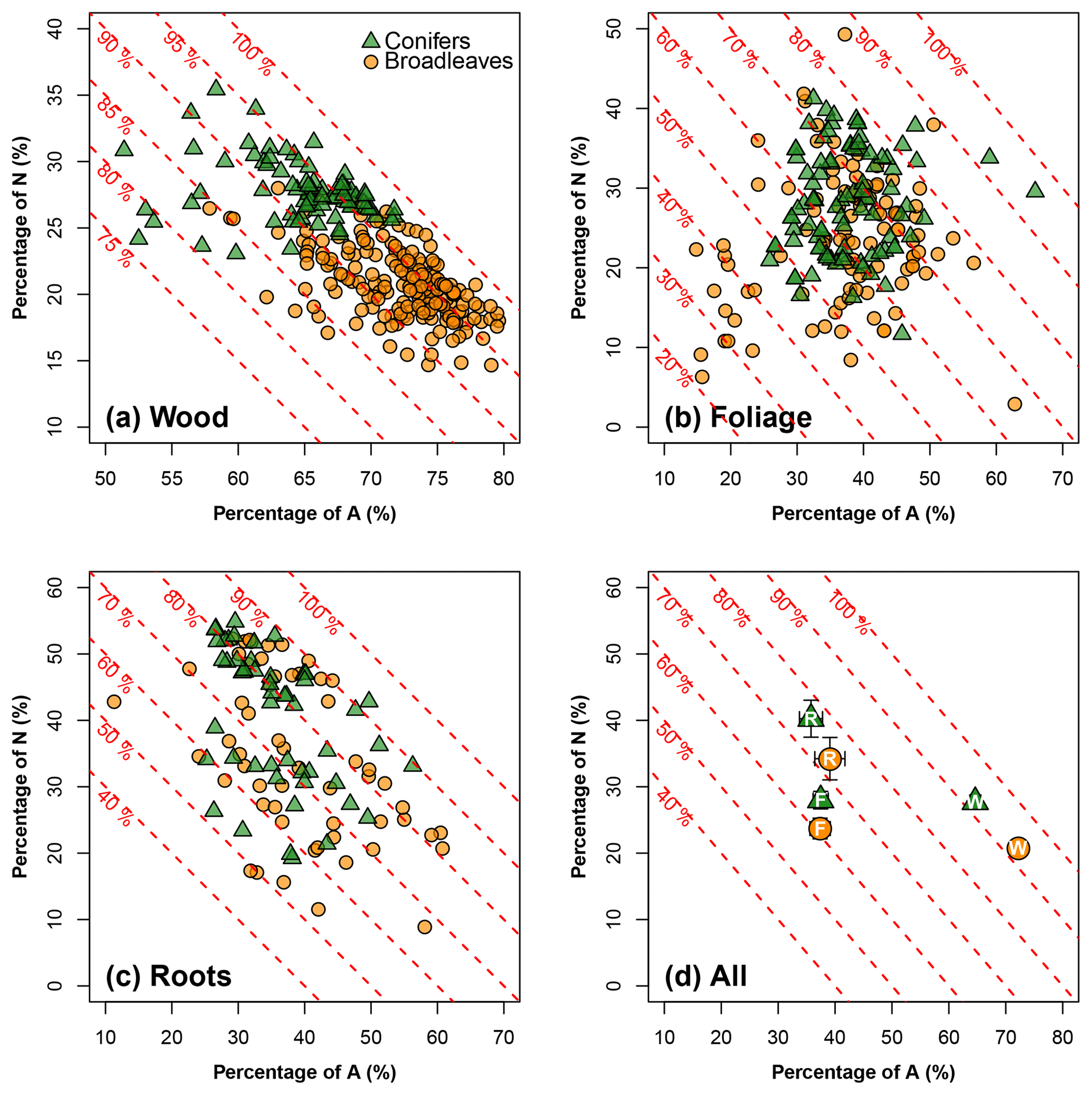
Figure 2A meta-analysis of the carbon composition for northern temperate tree species: the x axis represents the percentage of acid-hydrolyzable compounds (e.g., cellulose, noted as A; in %), and the y axis represents the percentage of non-soluble and non-hydrolyzable compounds (e.g., lignin, noted as N; in %). The oblique red dashed lines show the sum of A and N and their values. The remaining percentage, i.e., , refers to the portion of non-polar extractives, ethanol or dichloromethane compounds (E), and water soluble compounds (W). Analyses are conducted (a) for wood (106 data points for broadleaves, and 79 for conifers), (b) for foliage litter (106 data points for broadleaves, and 83 for conifers) and (c) for root litter (58 data points for broadleaves, and 49 for conifers). (d) is a statistical summary (symbols and means and error bars – 1.96 × SE) for wood (W), foliage (F) and roots (R) in a common coordinate system. Note the use of different axis graduations in each plot. See Supplement II for the data sources.
3.1 Litter carbon quality of northern temperate tree species
Our meta-analysis (Fig. 2) showed that the litter carbon quality, i.e., carbon composition, of northern temperate tree species significantly differed between tree organs. For woody litter (stem data alone), the A carbon pool reached up to 80 % of the total carbon pool; the sum of the A and N carbon pools corresponded to at least 75 % and, in most cases, was greater than 90 %. W and E accounted for only small percentages of the carbon composition (Fig. 2a). Nevertheless, this dominance of A and N over W and E was much less pronounced in foliage and root litter types (Fig. 2b and c). Generally, the different tree organs can be ranked according to the sum of the proportions of A and N as follows: woody debris (> 90 %) > roots (70 %–80 %) > foliage (60 %–70 %; Fig. 2d).
The effect of tree functional type on litter carbon quality strongly interacted with that of the tree organ. For wood, broadleaves and conifers had clearly shifted point clouds for the relationship between A and N carbon pools: there was a greater proportion of A and a lower proportion of N in broadleaves than in conifers. In foliage and root litter, the effect of tree functional type on the proportions of A and W was less pronounced than for wood. The main difference between broadleaves and conifers occurred in N rather than in A (Fig. 2d). Broadleaved litter had a smaller N proportion than coniferous litter, regardless of the tree organ (Fig. 2d). The proportions of A and N relative to those of E and W were quite stable between broadleaves and conifers regardless of the tree organ (Fig. 2d).
3.2 Sensitivity analyses on the impact of initial soil and litter settings on model output
Figure S3 shows the impact of different settings of litter and carbon quantity and quality on the model fit for the RENECOFOR sites. For soil carbon quality, the partial steady-state assumption (Fig. S3c and d) achieved significantly better model fits (with lower model root-mean-square-error) than the complete steady-state assumption (Fig. S3a and b). Next, we found that model fits were better when an observed CS to 0.4 m in depth (Fig. S3a and c) was used as the initial carbon quantity than when a CS to 1.0 m in depth was used (Fig. S3b and d). Nevertheless, it remained more advantageous to use the CS to 1.0 m observed during the first assessment as the model input because Yasso07 is calibrated to predict the CS down to 1.0 m in depth (Rantaraki et al., 2012).
Different choices of fine-root-to-foliage ratio for fine-root litter input also significantly influenced Yasso07's performance in predicting changes in soil C (Fig. S3). Ratios of 0.1–0.8 for broadleaves and 1.8–3.0 for conifers achieved the best fits between simulated and observed changes in the soil CS according to different scenarios (Fig. S3). Using a constant value of 1.0 for both broadleaved and coniferous sites seems to be an acceptable compromise between the two tree functional types, even though the choice is not optimal for each functional type taken individually.
As a result of the above diagnoses, we only show fit and residual analysis results for the simulations based on the partial steady-state assumption, observed CS to 1.0 m and fine-root-to-foliage ratio of 1.0 (see Fig. S3d and Sect. 3.3).
Figure S4 visualized all the theoretically possible final CSs by varying initial CSs and simulated duration (from 1 to 10 000 years). Initial soil carbon quality had a pronounced impact on final soil organic CSs at the annual and decennial scales. For example, when the initial proportion of the A pool increased from 0 % to 80 %, the final proportion of A could increase by +30 to +40 tC ha−1 (Fig. S4a) and the final total CSs could decrease by approximately −20 to −30 tC ha−1 (Fig. S4u) at annual and decennial scales. When simulations were performed for a millennium timescale, the initial soil carbon quality no longer impact final soil carbon quality. In other words, the same final soil carbon quality was obtained regardless of the initial soil quality (Fig. S4).
3.3 Simulated versus observed carbon data
Using only mean litter input, the theoretical CSs (CSsteady-state) simulated from the initialization method and the observed CS to 1.0 m in depth shared the same order of magnitude and were quite comparable (Fig. S5). However, the CSs were overestimated for most coniferous stands and underestimated for broadleaved stands (Fig. S5).
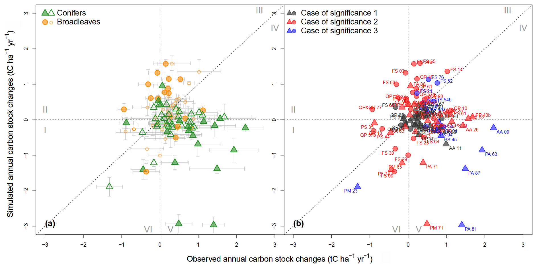
Figure 3Comparison between simulated and observed changes in annual carbon stocks (ACCs; in tC ha−1 yr−1). Circles and triangles represent sites dominated by broadleaves and conifers, respectively. The partial steady-state assumption was used when initializing CS quality to 1.0 m in depth. The fine-root-to-foliage ratio for broadleaves and conifers is 1.0. To facilitate readability, Roman numerals (I–VI) denote the six zones in which data points are distributed. In (a), error bars represent standard errors; hollow and filled points represent non-significant and significant differences, respectively, between simulated and observed ACCs according to the t test (at a 95 % confidence interval). In (b) the case of significance is as follows: 1 – no significant difference from 0 for either observed or simulated ACC; 2 – a significant difference from 0 for either observed or simulated ACC; and 3 – a significant difference from 0 for both observed and simulated ACC.
When simulated ACCs were plotted against the observed ones, the point clouds were distributed around the 1:1 diagonal line despite fairly high dispersion (Fig. 3). The correlation between predicted and measured ACC remained weak (R2<0.1). The mean observed and simulated ACCs for all sites were, respectively, tC ha−1 yr−1 ( tC ha−1 yr−1 for broadleaved stands and tC ha−1 yr−1 for coniferous stands) and tC ha−1 yr−1 ( tC ha−1 yr−1 for broadleaved stands and tC ha−1 yr−1 for coniferous stands); 23 % of the broadleaved stands and 39 % of the coniferous stands showed significant differences between observed and simulated ACCs (Fig. 3a). In only approximately 17 % of the sites, ACCs were significantly different from 0 for both simulated and observed results (i.e., case 3 in Fig. 3b). Here, there was a significant effect of tree functional type on the observed and simulated values. The model tended to overestimate ACC in broadleaved stands but to underestimate ACC in coniferous stands. Approximately two-thirds of all the sites showed predicted and observed changes in CSs of the same trend (i.e., data points in zones I, III, IV and VI; Fig. 3), while approximately one-third of the sites were in the remaining zones (II and V) where the predicted trend was contrary to the observed trend. From the residual distribution, we also found that the model where carbon quality was set with the partial steady-state assumption (Fig. 3) had a better fit than the model set with the complete steady-state assumption (Fig. S6).

Figure 4Observed (y axis; a) and simulated annual changes in carbon stocks (y axis; b) plotted against the CSs observed to 1.0 m in depth (x axis) during the first soil CS assessment. Regressions are as follows: (R2=0.03) for observed values at the sites dominated by broadleaves, (R2=0.01) for observed values at the sites dominated by conifers, (R2=0.62) for simulated values for the sites dominated by broadleaves and (R2=0.60) for simulated values for the sites dominated by conifers.
The simulated ACCs exhibited a negative linear relationship with the initial soil CSs (Fig. 4b), whereas this trend was not found for the observed ACCs (Fig. 4a). Storm damage and soil type could not clearly explain these trends in the residuals. For coniferous stands only, the residuals showed significant differences among the three major types of soil (n of sites > 5): cambisol > luvisol > podzol (Fig. S7). The coniferous stands tended to be younger than the broadleaved stands. Neither tree age nor the interaction between tree age and tree functional type had any significant effect on residuals. For all the sites together, the residuals became higher with increasing latitude, indicating that simulated ACCs were more overestimated in northern zones (analysis of covariance – ANCOVA; F=11.2, P < 0.001). This pattern was particularly strong for broadleaved stands (Fig. S8a). No similar trend was found for coniferous stands (Fig. S8e). Both residual signs were generally present for all of the main species (Fig. S8b, c, d, f, g and h). Broadleaved and coniferous stands differed in their responses to environmental factors: for coniferous stands, neither temperature nor precipitation had much effect on residuals, while for broadleaves, precipitation was negatively correlated with residuals (ANCOVA, F=10.8, P < 0.001).
Regarding soil physical and chemical properties, total soil nitrogen stocks were significantly correlated with residuals for both broadleaved and coniferous stands (Fig. 5). Soil texture (proportion of clay and sand) and exchangeable magnesium and potassium were significantly correlated with residuals only for broadleaved stands (Figs. 5 and S9; Table S2). The remaining tested variables, exchangeable aluminum and calcium, pH, total phosphorus and carbon-to-nitrogen ratio, showed no relationships with the residuals (Table S2).
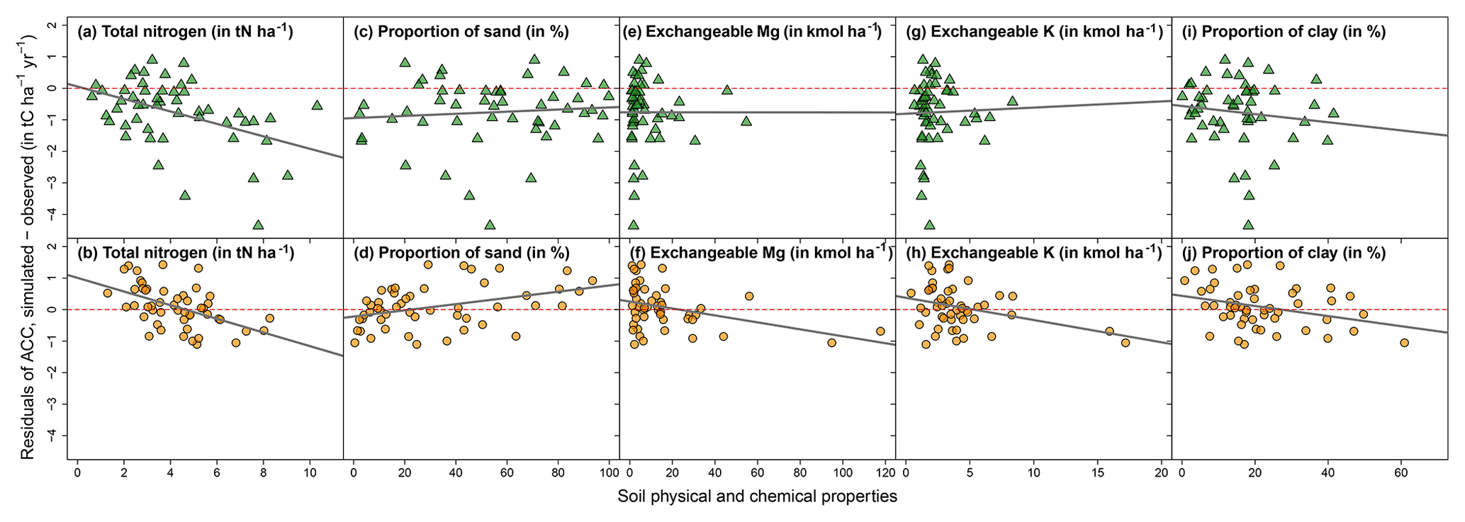
Figure 5Residuals of annual carbon stock change (ACC) plotted against selected soil physical and chemical properties. Top plots with green triangles represent sites dominated by conifers, and bottom plots with orange dots represent sites dominated by broadleaves. Regressions in all five subplots for the broadleaved sites (b, d, f, h, j) and in one subplot for the stands dominated by conifers (a) are significant (* P<0.5). See Table S2 for linear regression results for all 11 soil variables. Red dashed line indicates the zero line.
4.1 Agreement between simulated and observed annual changes in soil carbon stock
Testing widely popularized soil carbon models on a large dataset is highly meaningful work that enables researchers not only to assess the model's predictive ability over various climatic and ecosystem types but also to provide lessons and implications for future modeling work. Here, compared with observed CS data to 1.0 m in soil depth from the RENECOFOR network, we found that the simulated stocks (CSsteady-state versus CS) to 1.0 m showed the same order of magnitude and validated Yasso07's ability to predict average CSs at the scale of the French territory. This solid performance at the national scale supports Yasso's aim to be generalizable and is consistent with previous studies (see Ortiz et al., 2013; Lehtonen et al., 2016; Hernández et al., 2017). Nevertheless, the observed CS to 1.0 m in depth at t1 already exceeded the CSsteady-state for most coniferous stands (Fig. 5S), suggesting, to some extent, that the model parameters were not adapted to the RENECOFOR dataset. Such inadaptability may simply be due to setting an overly high decomposition rate for the slow carbon pools in the model. As the coniferous stands were on average younger being afforested more recently than the broadleaved stands (Jonard et al., 2017), the model may also not have been able to account for historic land use changes when the soil organic CS was calculated at the steady state. Figure S5 shows that for most broadleaved stands, observed stocks were lower than their CSsteady-state, possibly indicating that steady-state equilibrium had not yet been reached at these sites.
Furthermore, compared with the average observed ACCs over the 15-year interval between the two assessments, we found that the simulated ACCs were significantly biased for more than one-third of the French RENECOFOR sites. Particularly, Yasso07 generally overestimated the ACC in the broadleaved stands located in the north of France (Fig. S8a–d); this overestimation was sometimes exacerbated by lower precipitation. On the other hand, Yasso07 tended to underestimate the ACCs in the coniferous stands. Nevertheless, we expected Yasso07 to perform slightly better in the coniferous stands than in the broadleaved ones, since the model's estimates have shown good correspondence to measurements (of stocks and/or changes) in coniferous forests, especially Nordic boreal forests (e.g., Karhu et al., 2011; Ortiz et al., 2013). Probably due to the younger age of the coniferous stands in our study, the observed ACCs in the coniferous stands were greater than those in the broadleaved stands (Fig. 3; Jonard et al., 2017). Again, Yasso07 was unable to reproduce this observed effect of tree functional type on ACC, as the model does not take into account changes in land use history, as for the case of steady-state CSs mentioned above.
Except for tree functional type and geographical location (e.g., latitude, which is correlated with climatic variables), qualitative ecological variables that are assumed to be key factors influencing carbon sequestration processes (e.g., soil type – except for coniferous stands, storm damage and stand age range) showed limited ability to explain residuals. Note that these factors were not fully crossed for the 101 sites, making it difficult to test each single factor.
Simulated ACCs showed a strongly negative correlation with the observed initial soil CSs (CS), with an overestimation of ACC at sites with lower CS and an underestimation at sites with higher CS (Figs. 4 and S9). This is logical in view of the model's inherent mechanism. With increasing initial CS, there is an increase in the quantity of the easily decomposable compounds in the soil, i.e., A, W and E, which triggers a more substantial mass loss at a decennial scale. However, the data on observed changes in CSs did not support this trend.
Several quantitative soil physical and chemical properties showed clear correlations (especially for broadleaved stands) with ACC residuals (Fig. 5). Also, in the principle component analyses (Fig. S9), the arrows representing soil variables are slightly closer to the pivoting axis of “initial CS and ACC residuals” than those representing climatic and geographic variables, notably for broadleaved stands. These results highlight the potential interest of incorporating soil properties into new versions of the Yasso model, which currently lacks, or only implicitly incorporates, soil parameters. Indeed, there is considerable evidence that soil physical and chemical properties can greatly influence soil carbon dynamics and storage capacity (Beare et al., 2014; Dignac et al., 2017; Rasmussen et al., 2018).
Despite Yasso07's significant prediction bias at a number of sites, it is unreasonable to simply attribute the bias to the model per se, since multiple uncertainties affecting the quality of the model's input data can be identified (see Sect. 4.2–4.3). These uncertainties can occur not only with Yasso07 but also with other prevailing models, highlighting large knowledge gaps in ecology and soil carbon modeling.
4.2 Setting soil carbon quality for model initialization: a recurrent challenge in soil carbon modeling
Great uncertainty is associated with model initialization in terms of soil carbon quality, as it is usually estimated, not measured, for example, through matrix inversion with the assumption that the litter input has been the same for decades. Compared to measuring total soil CSs, measuring soil carbon quality is much more labor-intensive and time-consuming. Moreover, soil carbon quality data from different sources may be partly or totally incompatible due to the use of different chemical pools or fractionation protocols (Blair et al., 1995). Therefore, measured data for soil carbon quality are generally lacking at the worldwide scale. This lack of information is a recurrent issue for soil carbon dynamics modeling (see Elliot et al., 1996, who have discussed the issue of “measuring the modelable”). Many prevailing soil carbon models require setting carbon quality in addition to carbon quantity, e.g., Romul (Chertov et al., 2001), RothC (Coleman and Jenkinson, 1996), CENTURY versions (Parton et al., 1987; Metherell et al., 1993) and CBM-CFS3 (Kurz et al., 2009). Setting carbon quality in models inappropriately may greatly change CS predictions (Wutzler and Reichstein, 2007; Carvalhais et al., 2008, 2010).
In this study, soil carbon quality data were unavailable at the French RENECOFOR sites. We therefore tested both complete and partial steady-state assumptions for setting the initial carbon quality. Compared to the complete steady-state assumption, the partial steady-state assumption made it possible to account for slow-cycling pools, which could still be accumulating carbon, and fast cycling pools in equilibrium (Wutzler and Reichstein, 2007). We did not use the precise method proposed by Wutzler and Reichstein (2007) to estimate initial carbon quality due to a lack of information necessary for the decomposition–accumulation dynamics of the H pool. Instead, while we followed the same partial steady-state assumption, we revised the proportions of the N and H pools and assumed that the A, W and E pools were in equilibrium and equal to the simulated values. We also assumed that the sum of all pools at t1 was equal to the observed stock. We found that our partial steady-state assumption gave rise to generally better model fits than the complete steady-state assumption (Fig. S3; see also Figs. 3 and S6), indicating its good suitability to the RENECOFOR sites. When plotting CSstead-state against CSobs (Fig. S5), we found a discrepancy: while the CSobs values of most of the broadleaved stands were smaller than CSstead-state, the CSobs of most of the coniferous stands were greater than CSstead-state. This discrepancy was brought into the ACC fit when the complete steady-state assumption was adopted (Fig. S6). Nevertheless, the partial steady-state assumption can, to some extent, mitigate such a discrepancy. For broadleaved stands, the revised proportions of the A + W + E pools became higher than those at the complete steady state (Fig. 6; with 70 % of stands above the steady-state line), thus reducing the model's overestimation of ACC. For coniferous sites, the proportions of the A + W + E pools were often compressed (Fig. 6; with < 50 % of the stands above the steady-state strip), thus reducing the model's underestimation of ACC at the steady state.
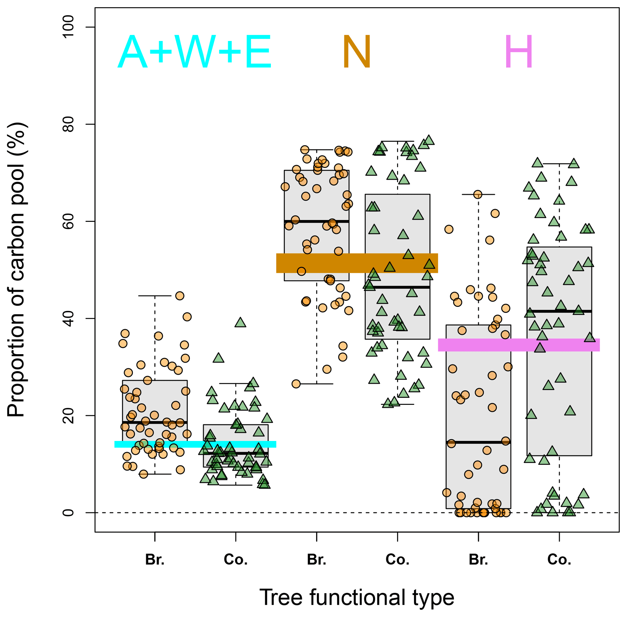
Figure 6Distribution of estimated carbon quality based on the partial steady-state assumption (box plots) versus those based on the complete steady-state assumption (whose ranges are all very narrow and are expressed with strips in color: 13 %–15 % for the sum of A, W and E – cyan; 49 %–53 % for N – brown; and 33 %–36 % for H – purple). For each box plot, the low and top edges of the box correspond to the 25th and 75th percentile data points, respectively; the line inside the box represents the median, and there are no outlier points in this case. Br. – broadleaved stands; Co. – coniferous stands.
For future work, it would definitely be worthwhile to compare both assumptions for several prevailing carbon models (e.g., Yasso07, RothC, Century, etc.), as studies comparing initialization assumptions still remain scarce compared to those on model comparisons.
In order to gain a global overview of Yasso07's sensitivity to initial soil carbon quality, we also conducted a sensitivity analysis that computed the final soil CSs for all possible chemical-pool compositions. This sensitivity analysis confirmed the high influence of initial soil carbon quality on soil CS estimates (Fig. S4), notably at short temporal scales (i.e., yearly and decennial). This result is in line with previous CS modeling studies (Parton et al., 1993; Kelly et al., 1997; Smith et al., 2009; Foereid et al., 2012), confirming that initialization is a crucial step for all chemical-pool-based carbon models. Our sensitivity analysis further showed that the effect of initial CS composition would gradually vanish with increasing length of time, especially in the case of several centuries or millennia. Our analysis provides new insights on the sensitivity of CS estimates to the method and assumptions used in model initialization. This analysis can be transposed to other carbon models to test their theoretical performance and robustness at different temporal scales and to compare models.
Finally, testing different initialization assumptions and performing sensitivity analyses are not enough to solve the predictability issues related to uncertainties in soil carbon quality. Based on ground truth data, Balesdent et al. (2018) showed that carbon age strongly reflects soil depth and ecosystem type. It appears to be highly necessary for future modeling work to capture better indicators of carbon stabilization mechanisms in the model initialization procedure. Yasso07's particular model configuration, i.e., based on measurable chemical pools, may make it possible to use measured soil carbon quality data for model initialization instead of steady-state assumptions. Future measurements of radiocarbon age for soil organic matter at the RENECOFOR sites may offer an ideal opportunity to compare the impact of initial soil carbon quality on Yasso07's predictions.
4.3 A precise estimation of root litter quantity helps improve Yasso07 predictions
An important source of uncertainty in the estimates of litter quantity at the RENECOFOR sites concerned fine-root litter input. Many studies have revealed that fine roots are a major source contributing to total litter quantity due to their fast turnover rates (Brunner et al., 2013; Kögel-Knabner et al., 2002; Berg and McClaugherty, 2008). In some forest ecosystems, the proportion of fine-root litter is even comparable to that of foliage (Freschet et al., 2013; Xia et al., 2015). However, estimating fine-root litter input is, again, a time-consuming and challenging task. For this reason, to our best knowledge, probably no nationwide forest inventory projects have ever incorporated direct measurements of the dynamics of fine-root litter input (and this information is also lacking for the RENECOFOR network). Fine root turnover for forest species varies depending on climate, tree species and management scenarios (Kögel-Knabner et al., 2002; Litton et al., 2003; Mokany et al., 2006), and this makes choosing model input values highly subjective and difficult. By testing variable fine-root-to-foliage ratios of litter input, we observed a significant shift in the ACCs predicted by Yasso07 (Fig. S3). This finding not only highlights the importance of precisely quantifying fine-root litter input but also suggests that broadleaves and conifers may have a different fine-root litter input ratio with regard to that of foliage, although we chose the same ratio for both broadleaved and coniferous stands in this study. It should be noted that using one ratio per tree functional type (conifers versus broadleaves) can only change the overall prediction baseline and cannot reduce data dispersion. Consequently, it is of great interest to estimate fine-root litter input quantity at the species level through direct measurements and then couple the specific data with Yasso07.
Potentially important litter input may also come from the shrubby and herbaceous understory species, which we did not take into account in this study due to data unavailability. The herb and shrub layers are typically not included in forest inventories, though they can contribute significantly to the annual litter production in forests (e.g., de Wit et al., 2006; Gilliam, 2007; Lehtonen et al., 2016). Muukkonen and Mäkipää (2006) estimated that the carbon input from herbaceous and shrub vegetation in Finnish forests was from 0.50 to 0.66 tC ha−1 yr−1. This is quite high, as the value represents of the mean total tree litter input for all the RENECOFOR sites combined (Table 1). This is in line with data from Didion et al. (2018), who estimated that understory vegetation at the sites of the Swiss National Forest Inventory contributed on average 10 %–15 % to the total observed annual non-woody carbon turnover with a range from a few percent to more than 50 %.
Finally, Yasso07's parameter set was calibrated based on one of the richest litterbag datasets in the world in terms of number of observations. The state of the art of soil carbon modeling assumes that litter input and decomposition processes are the driving forces in soil carbon accumulation. However, other important sources of biological carbon input exist, e.g., soil fauna and rhizodeposition; unfortunately, our ability to take them into account in modeling processes remains poor. Whether, and to what extent, the bias found in our Yasso07 results is related to these alternative sources of biological carbon input is unknown.
4.4 Suggestions for future modeling improvements
First, we found the Yasso07 model structure and algorithm solid, clear and simple to operate, in agreement with the positive remarks in the literature (Rantakari et al., 2012; Didion et al., 2014; Lu et al., 2015; Wu et al., 2015). Regarding its mass flow parameters, Fig. S1 only shows the mass flows that are statistically significant in the case of the Tuomi (2011) parameter set. Yasso07 keeps all the theoretical mass flow possibilities in the Ap matrix in (Eq. 1b). However, a mass flow parameter with a statistical significance does not signify that it is biologically meaningful. For example, we can quote the flow N → A in the model (Fig. S1), for which the modeler assigned an astonishingly high percentage: %. This quantity is disputable in light of soil biochemistry, because lignin, the major component constituting the N carbon pool, is not likely to pass into the A pool but would instead probably condense with other nearby phenols, peptides or saccharides (Burns et al., 2013).
As a model for predicting soil carbon dynamics, Yasso07 is still overly simple in the description of some soil variables that are known to strongly impact decomposition processes. For example, soil mineralogy or aggregation is yet to be accounted for in Yasso07. Indeed, the model has often been applied on soils fairly rich in organic matter (e.g., Karhu et al., 2011), where the consideration of soil mineral properties was not particularly relevant and where the authors' assumption that litter quantity is a good proxy for soil properties was reasonable. In addition, when Yasso, Yasso07's prototype, was published in 2005 (Liski et al., 2005), information on mineral soil properties in the various forest soil horizons was not commonly available. Nowadays, however, it is easier to obtain, although there is still not enough detailed data for consistent application across large regions or at the national scale (Didion et al., 2016).
We tested the performance of the Yasso07 soil carbon model on decennial-scale French nationwide forest data collected through the RENECOFOR network. We also compiled a meta-analysis database for litter carbon quality and carried out sensitivity analyses to characterize the effect of initial litter input and soil carbon quality on the model's predictions. We showed that, while the model's estimates of CS to 1.0 m in depth and of ACC stayed within the same order of magnitude as observed values, the accordance between the observed and simulated ACCs at the site scale remained weak. There was a bias in the model's predicted trends for changes in CS at more than one-third of the French sites. As we have shown for Yasso07, the performance of soil carbon models should be examined before their application to management guidelines and policymaking for forest ecosystems at any scales.
Biases can be attributed to multiple factors concerning model input, such as (i) uncertainty in the measurement data for soil CSs and changes, (ii) a lack of information on initial soil carbon quality at the site level, and (iii) a lack of information on below-ground litter production. These factors are valid for the state-of-the-art soil carbon modeling, regardless of the model that one uses. Our sensitivity analyses explicitly confirmed the importance of factors (i) and (ii) above. Appropriately setting soil carbon quality is one of the most crucial steps to guarantee the model's fit. We found that the partial steady-state assumption gives rise to a significantly better model fit than does the complete steady-state assumption, when setting soil carbon quality. Some of the model's parameters governing the transfer among soil pools are statistically derived and not directly measured and thus may poorly represent actual biochemical decomposition processes. Residual analysis also suggests a potentially important role of physical and chemical soil properties in explaining the model's prediction ability.
Our findings allow us to provide modelers, users and policymakers with the following suggestions:
-
We suggest that Yasso07 modelers keep the current model structure, algorithm and parameters but incorporate some more refined biochemical processes: for example, that they (i) revise certain mass flows to achieve both statistically and biologically meaningful processes (especially the N → A flow), (ii) refine the decomposition process (i.e., the residence times between the A, W and E soil carbon pools); and, possibly, (iii) explicitly incorporate easily measured soil parameters to better represent biophysical and biochemical interactions in soil carbon cycling.
-
We suggest that Yasso07 users work in conjunction with modelers in order to better reduce the uncertainties in model initialization for soil CSs. We also suggest measuring forest carbon quality and quantity and below-ground fine-root litter to better feed the model.
-
We suggest that policymakers remain prudent toward diagnoses based on a single carbon model, especially when a long-term trend is predicted. Predictions from multiple models should be cross-validated for both global and local areas.
This study, involving decennial observations at sites spread over a large spatial scale and covering different ecosystems, provides a good opportunity to facilitate future model calibration, improvement and reassessment. Finally, with Yasso07 as an example, this work highlighted the bottleneck in soil carbon modeling caused by the lack of knowledge or data on soil and litter carbon quality and on fine-root litter quantity, which creates high uncertainties for model initialization. Simultaneously, we demonstrated methodologies for testing other soil carbon models via sensitivity analyses to better enable us to understand the limits of the model and of the input data and to plan future improvements in soil organic carbon modeling. In this study, we used the model structure and parameters published in Tuomi et al. (2011a) without any modifications. Further work on sensitivity analyses incorporating modifications in both the carbon quality and litter input settings and Yasso07's configuration and parameters is needed to confirm the reliability of the current diagnoses.
The plant and soil data used for model fit and validation are those published in Jonard et al. (2017). These data can be accessible via contacting the RENECOFOR network (http://www.onf.fr/renecofor (Office national des forêts, 2019)., last access: 21 April 2019).
| Name | Meaning |
|---|---|
| Carbon stock (CS) | Quantity of organic carbon stocked in the soil (in tC ha−1) |
| Carbon stock change | Increment (positive value) or decrement (negative value) of organic carbon stocked in the soilbetween year t1 and year t2 (in tC ha−1) |
| Annual carbon stockchange (ACC) | Change in CSs per year (in tC ha−1 yr−1) |
| Carbon pools | The Yasso07 model contains a series of organic compounds involved in decomposition processes differing in solubility and mean residence time: water soluble compounds (W), acid-hydrolyzable compounds (A), non-polar solvent, ethanol or dichloromethane compounds (E), and non-soluble and non-hydrolyzable compounds (N). For soil, there is an additional recalcitrant pool called “humus” (H). Note that in this paper, “N” only denotes non-soluble and non-hydrolyzable compounds; nitrogen is spelled in full when mentioned. |
| Coarse woody litter | Litter originating from either coarse above-ground residues due to either harvests or storms (including coarse branches of > 4 cm in diameter and miscellaneous residues) and coarse roots of >5 mm in diameter |
| Fine non-woody litter | Litter originating from either natural above-ground litterfall (leaves, small branches) or fine-root activities |
| Litter carbon quality | Litter carbon (in %) belonging to the A, W, E and N carbon pools (see “carbon pools” above) |
| Litter quantity | Annual litter accumulation (in tC ha−1 yr−1) |
| Soil carbon quality | Soil carbon (in %) belonging to the A, W, E, N and H carbon pools |
The supplement related to this article is available online at: https://doi.org/10.5194/bg-16-1955-2019-supplement.
DD, MD and LSA designed the study as well as the structure of the paper. ZM, MD, MN and LSA collected or provided the data. JL provided technical help for model use. ZM performed model simulation, data analysis and wrote the first draft. DD, MD, TE and LSA participated in data analysis and result interpretation. All the co-authors participated in paper preparation.
The authors declare that they have no conflict of interest.
This study was funded by the French Agence de l'Environnement et de la Maîtrise de l'Energie (ADEME; contract reference: 14-60-C0082). The UR1138 BEF and this study were supported by a grant overseen by the French National Research Agency (ANR) as part of the “Investissements d'Avenir” program (ANR-11-LABX-0002-01, Laboratory of Excellence ARBRE) – QLSPIMS project. This study is an outcome of a project entitled “Input to improve the comparability in MRV across EU MS” within the LULUCF MRV project “Analysis of and proposals for enhancing Monitoring, Reporting and Verification (MRV) of land use, land use change and forestry (LULUCF) in the EU” funded by the European Commission. Funding for Markus Didion was provided by the Swiss Federal Office for the Environment. We thank several French colleagues, Isabelle Feix (ADEME), Arnaud Legout (INRA) and Bertrand Guenet (CNRS), for their valuable comments. We are also grateful to Anna Repo (FEI – SYKE) and Emmi Hilasvuori (FEI – SYKE) for their explanations of Yasso07 and to Victoria Moore for her thorough review and suggestions for improving the English language.
This paper was edited by Luo Yu and reviewed by Thomas Wutzler and one anonymous referee.
Aber, J. D., Melillo, J. M., and McClaugherty, C. A.: Predicting long-term patterns of mass loss, nitrogen dynamics, and soil organic matter formation from initial fine litter chemistry in temperate forest ecosystems, Can. J. Bot., 68, 2201–2208, https://doi.org/10.1139/b90-287, 1990.
Aulen, M., Shipley, B., and Bradley, R.: Prediction of in situ root decomposition rates in an interspecific context from chemical and morphological traits, Ann. Bot.-London, 109, 287–297, https://doi.org/10.1093/aob/mcr259, 2011.
Balesdent, J., Basile-Doelsch, I., Chadoeuf, J., Cornu, S., Derrien, D., Fekiacova, Z., and Hatté, C.: Atmosphere–soil carbon transfer as a function of soil depth, Nature, 559, 599–602, https://doi.org/10.1038/s41586-018-0328-3, 2018.
Beare, M., McNeill, S., Curtin, D., Parfitt, R., Jones, H., Dodd, M., and Sharp, J: Estimating the organic carbon stabilisation capacity and saturation deficit of soils: a New Zealand case study, Biogeochemistry, 120, 71–87, https://doi.org/10.1007/s10533-014-9982-1, 2014.
Berg, B. and McClaugherty, C.: Plant litter: decomposition, humus formation, carbon sequestration, 2nd Edn., Springer-Verlag Heidelberg Berlin, 286 pp., https://doi.org/10.5860/choice.51-6172, 2008.
Brunner, I., Bakker, M. R., Björk, R. G., Hirano, Y., Lukac, M., Aranda, X., Børja, I., Eldhuset, T. D., Helmisaari, H. S., Jourdan, C., Konôpka, B., López, B. C., Miguel Pérez, C., Persson, H., and Ostonen, I.: Fine-root turnover rates of European forests revisited: an analysis of data from sequential coring and ingrowth cores, Plant Soil, 362, 357–372, https://doi.org/10.1007/s11104-012-1313-5, 2013.
Burns, R. G., DeForest, J. L., Marxsen, J., Sinsabaugh, R. L., Stromberger, M. E., Wallenstein, M. D., Weintraub, M. N., and Zoppini, A.: Soil enzymes in a changing environment: current knowledge and future directions, Soil Biol. Biochem., 58, 216–234, https://doi.org/10.1016/j.soilbio.2012.11.009, 2013.
Carvalhais, N., Reichstein, M., Seixas, J., Collatz, G. J., Pereira, J. S., Berbigier, P., Carrara, A., Granier, A., Montagnani, L., Papale, D., and Rambal, S.: Implications of the carbon cycle steady state assumption for biogeochemical modeling performance and inverse parameter retrieval, Global Biogeochem. Cy., 22, GB2007, https://doi.org/10.1029/2007gb003033, 2008.
Carvalhais, N., Reichstein, M., Ciais, P., Collatz, G.J., Mahecha, M.D., Montagnani, L., Papale, D., Rambal, S., and Seixas, J.: Identification of vegetation and soil carbon pools out of equilibrium in a process model via eddy covariance and biometric constraints, Glob. Change Biol., 16, 2813–2829, https://doi.org/10.1111/j.1365-2486.2010.02173.x, 2010.
Chertov, O. G., Komarov, A. S., Nadporozhskaya, M., Bykhovets, S. S., and Zudin, S. L.: ROMUL – a model of forest soil organic matter dynamics as a substantial tool for forest ecosystem modeling, Ecol. Model., 138, 289–308, https://doi.org/10.1016/s0304-3800(00)00409-9, 2001.
Coleman, K. and Jenkinson, D. S.: RothC-26.3 – A Model for the turnover of carbon in soil, in: Evaluation of Soil organic matter models, Using Existing Long-Term Datasets, edited by: Powlson, D. S., Smith, P., and Smith, J. U., Springer-Verlag, Heidelberg, 237–246, https://doi.org/10.1007/978-3-642-61094-3_17, 1996.
Didion, M., Frey, B., Rogiers, N., and Thürig, E.: Validating tree litter decomposition in the Yasso07 carbon model, Ecol. Model., 291, 58–68, https://doi.org/10.1016/j.ecolmodel.2014.07.028, 2014.
Didion, M., Blujdea, V., Grassi, G., Hernández, L., Jandl, R., Kriiska, K., Lehtonen, A., and, Saint-André, L.: Models for reporting forest litter and soil C pools in national greenhouse gas inventories: methodological considerations and requirements, Carbon Manag., 7, 1–14, https://doi.org/10.1080/17583004.2016.1166457, 2016.
Didion, M., Baume, M., Giudici, F., and Schneuwly, J.: Herb layer biomass in Swiss forests. 53 pages. Swiss Federal Research Institute WSL, Biirmensdorf (ZH), https://doi.org/10.16904/envidat.52, 2018.
Dignac, M. F., Derrien, D., Barré, P., Barot, S., Cécillon, L., Chenu, C., Chevallier, T., Freschet, G. T., Garnier, P., Guenet, B., and Hedde, M: Increasing soil carbon storage: mechanisms, effects of agricultural practices and proxies, A review, Agron. Sustain. Dev., 37, 14, https://doi.org/10.1007/s13593-017-0421-2, 2017.
Fox, J. and Weisberg, S.: Nonparametric Regression in R: An Appendix to An R Companion to Applied Regression, 3rd Edn., Sage, Thousand Oaks, CA, 17 pp., 2019.
Freschet, G. T., Cornwell, W. K., Wardle, D. A., Elumeeva, T. G., Liu, W., Jackson, B. G., Onipchenko, V. G., Soudzilovskaia, N. A., Tao, J., and Cornelissen, J. H. C.: Linking litter decomposition of above and below ground organs to plant–soil feedbacks worldwide, J. Ecol., 101, 943–952, https://doi.org/10.1111/1365-2745.12092, 2013.
Guo, D. L., Mitchell, R. J., and Hendricks, J. J.: Fine root branch orders respond differentially to carbon source-sink manipulations in a longleaf pine forest, Oecologia, 140, 450–457, https://doi.org/10.1007/s00442-004-1596-1, 2004.
Hernández, L., Jandl, R., Blujdea, V. N. B., Lehtonen, A., Kriiska, K., Alberdi, I., Adermann, V., Cañellas, I., Marin, G., Moreno-Fernández, D., Ostonen, I., Varik, M., and Didion, M.: Towards complete and harmonized assessment of soil carbon stocks and balance in forests: The ability of the Yasso07 model across a wide gradient of climatic and forest conditions in Europe, Sci. Total Environ., 599/600, 1171–1180, https://doi.org/10.1016/j.scitotenv.2017.03.298, 2017.
IPCC: Use of Models and Facility-Level Data in Greenhouse Gas Inventories (Report of IPCC Expert Meeting on Use of Models and Measurements in Greenhouse Gas Inventories 9–11 August 2010, Sydney, Australia), Institute for Global Environmental Strategies (IGES), Hayama, Japan, 2011.
IPCC: Climate Change 2014: Mitigation of Climate Change, Contribution of Working Group III to the Fifth Assessment Report of the Intergovernmental Panel on Climate Change, edited by: Edenhofer, O., Pichs-Madruga, R., Sokona, Y., Farahani, E., Kadner, S., Seyboth, K., Adler, A., Baum, I., Brunner, S., Eickemeier, P., Kriemann, B., Savolainen, J., Schlömer, S., von Stechow, C., Zwickel, T., and Minx, J. C.: Cambridge University Press, Cambridge, United Kingdom and New York, NY, USA, 2014.
Jandl, R., Rodeghiero, M., Martinez, C., Cotrufo, M. F., Bampa, F., van Wesemael, B., Harrison, R. B., Guerrini, I. A., Richter, D. D., Rustad, L., Lorenz, K., Chabbi, A., and Miglietta, F.: Current status, uncertainty and future needs in soil organic carbon monitoring, Sci. Total Environ., 468, 376–383, 2014.
Jonard, M., Nicolas, M., Coomes, D. A., Caignet, I., Saenger, A., and Ponette, Q.: Forest soils in France are sequestering substantial amounts of carbon, Sci. Total Environ., 574, 616–628, https://doi.org/10.1016/j.scitotenv.2016.09.028, 2017.
Karhu, K., Wall, A., Vanhala, P., Liski, J., Esala, M., and Regina, K.: Effects of afforestation and deforestation on boreal soil carbon stocks – comparison of measured C stocks with Yasso07 model results, Geoderma, 164, 33–45, https://doi.org/10.1016/j.geoderma.2011.05.008, 2011.
Kelly, R. H., Parton, W. J., Crocker, G. J., Grace, P. R., Klír, J., Körschens, M., Poulton, P. R., and Richter, D. D.: Simulating trends in soil organic carbon in long-term experiments using the Century model, Geoderma, 81, 75–90, https://doi.org/10.1016/s0016-7061(97)00082-7, 1997.
Kögel-Knabner, I.: The macromolecular organic composition of plant and microbial residues as inputs to soil organic matter, Soil Biol. Biochem., 34, 139–162, https://doi.org/10.1016/s0038-0717(01)00158-4, 2002.
Krinner, G., Viovy, N., de Noblet-Ducoudré, N., Ogée, J., Polcher, J., Friedlingstein, P., Ciais, P., Sitch, S., and Prentice, I. C.: A dynamic global vegetation model for studies of the couple atmosphere-biosphere system, Global Biogeochem. Cy., 19, GB1015, https://doi.org/10.1029/2003gb002199, 2005.
Kurz, W. A., Dymond, C. C., White, T. M., Stinson, G., Shaw, C. H., Rampley, G. J., Smyth, C., Simpson, B. N., Neilson, E. T., Trofymow, J. A., and Metsaranta, J.: CBM-CFS3: a model of carbon-dynamics in forestry and land-use change impdlementing IPCC standards, Ecol. Model., 220, 480–504, https://doi.org/10.1016/j.ecolmodel.2008.10.018, 2009.
Lehmann, J. and Kleber, M.: The contentious nature of soil organic matter, Nature, 528, 60–68, https://doi.org/10.1038/nature16069, 2015.
Lehtonen, A., Linkosalo, T., Peltoniemi, M., Sievänen, R., Mäkipää, R., Tamminen, P., Salemaa, M., Nieminen, T., Tupek, B., Heikkinen, J., and Komarov, A.: Forest soil carbon stock estimates in a nationwide inventory: evaluating performance of the ROMULv and Yasso07 models in Finland, Geosci. Model Dev., 9, 4169–4183, https://doi.org/10.5194/gmd-9-4169-2016, 2016.
Liski, J., Palosuo, T., Peltoniemi, M., and Sievänen, R.: Carbon and decomposition model Yasso for forest soils, Ecol. Model., 189, 168–182, https://doi.org/10.1016/j.ecolmodel.2005.03.005, 2005.
Litton, C. M., Ryan, M. G., Tinker, D. B., and Knight, D. H.: Belowground and aboveground biomass in young postfire lodgepole pine forests of contrasting tree density, Can. J. Forest Res., 33, 351–363, https://doi.org/10.1139/x02-181, 2003.
Lu, N., Akujärvi, A., Wu, X., Liski, J., Wen, Z., Holmberg, M., Feng, X., Zeng, Y., and Fu, B.: Changes in soil carbon stock predicted by a process-based soil carbon model (Yasso07) in the Yanhe watershed of the Loess Plateau, Landscape Ecol., 30, 399–413, https://doi.org/10.1007/s10980-014-0132-x, 2015.
Manzoni, S. and Porporato, A.: Soil carbon and nitrogen mineralization: theory and models across scales, Soil Biol. Biochem., 41, 1355–1379, https://doi.org/10.1016/j.soilbio.2009.02.031, 2009.
Metherell, A., Harding, L. A., Cole, C. V., and Parton, W. J.: Technical Documentation Agroecosystem Version 4.0, Great Plains, System Research Unit, USDA-ARS, Fort Collins, CO, 1993.
Mokany, K., Raison, R., and Prokushkin, A. S.: Critical analysis of root: shoot ratios in terrestrial biomes, Glob. Change Biol., 12, 84–96, https://doi.org/10.1111/j.1365-2486.2005.001043.x, 2006.
Muukkonen, P. and Mäkipää, R.: Empirical biomass models of understorey vegetation in boreal forests according to stand and site attributes, Boreal Environ. Res., 11, 355–369, 2006.
Office national des forêts: Renecofor, available: http://www1.onf.fr/renecofor, last access: 21 April 2019.
Ortiz, C. A., Liski, J., Gärdenäs, A. I., Lehtonen, A., Lundblad, M., Stendahl, J., Ågren, G. I., and Karltun, E.: Soil organic carbon stock changes in Swedish forest soils – a comparison of uncertainties and their sources through a national inventory and two simulation models, Ecol. Model., 251, 221–231, https://doi.org/10.1016/j.ecolmodel.2012.12.017, 2013.
Parton, W. J., Schimel, D. S., Cole, C. V., and Ojima, D. S.: Analysis of factors controlling soil organic-matter levels in Great-Plains grasslands, Soil Sci. Soc. Am. J., 51, 1173–1179, https://doi.org/10.2136/sssaj1987.03615995005100050015x, 1987.
Parton, W. J., Scurlock, J. M. O., and Ojima, D. S.: Observations and modeling of biomass and soil organic matter dynamics for the grassland biome worldwide, Global Biogeochem. Cy., 7, 785–809, https://doi.org/10.1029/93gb02042, 1993.
Pettersen, R. C.: The chemical composition of wood, The chemistry of solid wood, 207, 57–126, 1984.
Raich, J. W. and Nadelhoffer, K. J.: Below-ground carbon allocation in forest ecosystems: global trends, Ecology, 70, 1346–1354, https://doi.org/10.2307/1938194, 1989.
Rantakari, M., Lehtonen, A., Linkosalo, T., Tuomi, M., Tamminen, P., Heikkinen, Liski J., Mäkipää R., Ilvesniemi H., and Sievänen, R.: The Yasso07 soil carbon model–Testing against repeated soil carbon inventory, Forest Ecol. Manag., 286, 137–147, https://doi.org/10.1016/j.foreco.2012.08.041, 2012.
Rasmussen, C., Heckman, K., Wieder, W., Keiluweit, M., Lawrence, C., Berhe, A., Blankinship, J., Crow, S., Druhan, J., Pries, C., Marin-Spiotta, E., Plante, A., Schädel, C., Schimel, J., Sierra, C., Thompson, A., and Wagai, R.: Beyond clay: towards an improved set of variables for predicting soil organic matter content, Biogeochemistry, Springer, Nature, 137, 297–306, https://doi.org/10.1007/s10533-018-0424-3, 2018.
Rowell, R. M. (Ed.): Handbook of wood chemistry and wood composites, CRC press, 487 pp., https://doi.org/10.1201/b12487, 2012.
Rowell, R. M., Pettersen, R., Han, J. S., Rowell, J. S., and Tshabalala, M. A.: Cell wall chemistry, in: Handbook of Wood Chemistry and Wood Composites, edited by: Rowell, R. M., CRC & Taylor & Francis, Boca Raton, Fla, USA, 35–74, https://doi.org/10.1201/b12487-5, 2005.
Saby, N. P. A., Bellamy, P. H., Morvan, X., Arrouays, D., Jones, R. J. A., Verheijen, F. G. A., Kibblewhite, M. G., Verdoodt, A. N. N., ÜVeges, J. B., Freudenschuß, A., and Simota, C.: Will European soil-monitoring networks be able to detect changes in topsoil organic carbon content?, Glob. Change Biol., 14, 2432–2442, https://doi.org/10.1111/j.1365-2486.2008.01658.x, 2008.
Schmidt, M. W. I., Torn, M. S., Abiven, S., Dittmar, T., Guggenberg, G., Janssens, I. A., Kleber, M., Kögel-Knabner, I., Lehmann, J., Manning, M., Nannipieri, P., Rasse, D. P., Weiner, S., and Trumbore, S. E.: Persistence of soil organic matter as an ecosystem property, Nature, 478, 49–56, https://doi.org/10.1038/nature10386, 2011.
Smith, W. N., Grant, B. B., Desjardins, R. L., Qian, B., Hutchinson, J., and Gameda, S.: Potential impact of climate change on carbon in agricultural soils in Canada 2000–2099, Climatic Change, 93, 319–333, https://doi.org/10.1007/s10584-008-9493-y, 2009.
Stump, L. M. and Binkley, D.: Relationships between litter quality and nitrogen availability in Rocky Mountain forests, Can. J. Forest Res., 23, 492–502, https://doi.org/10.1139/x93-067, 1993.
Thomas, S. C. and Martin, A. R.: Carbon content of tree tissues: a synthesis, Forests, 3, 332–352, https://doi.org/10.3390/f3020332, 2012.
Tingey, D. T., Mckane, R. B., Olszyk, D. M., Johnson, M. G., Rygiewicz, P. T., and Henry Lee, E.: Elevated CO2 and temperature alter nitrogen allocation in Douglas-fir, Glob. Change Biol., 9, 1038–1050, https://doi.org/10.1046/j.1365-2486.2003.00646.x, 2003.
Todd-Brown, K. E. O., Hopkins, F. M. H., Kivlin, S. N., Talbot, J. M., and Allison, S. D., A framework for representing microbial decomposition in coupled climate models, Biogeochemistry, 109, 19–33, https://doi.org/10.1007/s10533-011-9635-6, 2012.
Tuomi, M., Thum, T., Järvinen, H., Fronzek, S., Berg, B., Harmon, M., Trofymow, J. A., Sevanto, S., and Liski, J.: Leaf litter decomposition – Estimates of global variability based on Yasso07 model, Ecol. Model., 220, 3362–3371, https://doi.org/10.1016/j.ecolmodel.2009.05.016, 2009.
Tuomi, M., Laiho, R., Repo, A., and Liski, J.: Wood decomposition model for boreal forests, Ecol. Model., 222, 709–718, https://doi.org/10.1016/j.ecolmodel.2010.10.025, 2011a.
Tuomi, M., Rasinmaki, J., Repo, A., Vanhala, P., and Liski, J.: Soil carbon model Yasso07 graphical user interface, Environ. Modell. Softw., 26, 1358–1362, https://doi.org/10.1016/j.envsoft.2011.05.009, 2011b.
Wu, X., Akujärvi, A., Lu, N., Liski, J., Liu, G., Wang, Y., Holmberg, M., Li, F., Zeng, Y., and Fu, B.: Dynamics of soil organic carbon stock in a typical catchment of the Loess Plateau: comparison of model simulations with measurements, Landscape Ecol., 30, 381–397, https://doi.org/10.1007/s10980-014-0110-3, 2015.
Wutzler, T. and Reichstein, M.: Soils apart from equilibrium – consequences for soil carbon balance modelling, Biogeosciences, 4, 125–136, https://doi.org/10.5194/bg-4-125-2007, 2007.
Wutzler, T. and Reichstein, M.: Priming and substrate quality interactions in soil organic matter models, Biogeosciences, 10, 2089–2103, https://doi.org/10.5194/bg-10-2089-2013, 2013.
Xia, M., Talhelm, A. F., and Pregitzer, K. S.: Fine roots are the dominant source of recalcitrant plant litter in sugar maple-dominated northern hardwood forests, New Phytol., 208, 715–726, https://doi.org/10.1111/nph.13494, 2015.