the Creative Commons Attribution 4.0 License.
the Creative Commons Attribution 4.0 License.
 | 06 May 2019
Reciprocal bias compensation and ensuing uncertainties in model-based climate projections: pelagic biogeochemistry versus ocean mixing
Ulrike Löptien
Heiner Dietze
Anthropogenic emissions of greenhouse gases such as CO2 and N2O impinge on the Earth system, which in turn modulates atmospheric greenhouse gas concentrations. The underlying feedback mechanisms are complex and, at times, counterintuitive. So-called Earth system models have recently matured to standard tools tailored to assess these feedback mechanisms in a warming world. Applications for these models range from being targeted at basic process understanding to the assessment of geo-engineering options. A problem endemic to all these applications is the need to estimate poorly known model parameters, specifically for the biogeochemical component, based on observational data (e.g., nutrient fields). In the present study, we illustrate with an Earth system model that through such an approach biases and other model deficiencies in the physical ocean circulation model component can reciprocally compensate for biases in the pelagic biogeochemical model component (and vice versa). We present two model configurations that share a remarkably similar steady state (based on ad hoc measures) when driven by historical boundary conditions, even though they feature substantially different configurations (parameter sets) of ocean mixing and biogeochemical cycling. When projected into the future the similarity between the model responses breaks. Metrics such as changes in total oceanic carbon content and suboxic volume diverge between the model configurations as the Earth warms. Our results reiterate that advancing the understanding of oceanic mixing processes will reduce the uncertainty of future projections of oceanic biogeochemical cycles. Related to the latter, we suggest that an advanced understanding of oceanic biogeochemical cycles can be used for advancements in ocean circulation modules.


Challenges associated with climate change have triggered a discussion of geo-engineering to combat negative effects of anthropogenic greenhouse gas emissions on our planet. Among these options are ideas to purposely change pelagic biogeochemical cycles in order to increase oceanic carbon sequestration from the atmosphere (e.g., Williamson et al., 2012). Currently, the effectiveness and potential side effects of such measures are quantified with numerical Earth system models (e.g., Yool et al., 2009; Dutreuil et al., 2009; Oschlies et al., 2010) – tools known to be associated with substantial uncertainty (e.g., Bopp, 2013; Friedlingstein et al., 2014). One source of uncertainty in these models is related to unknowns in the mathematical representation (typically a set of partial differential equations) of both the physical and biogeochemical processes impacting the pelagic ocean.
As for the biogeochemical processes, considerable uncertainty is associated with poorly known model parameters (e.g., Kriest et al., 2010; Löptien and Dietze, 2017), such as growth rates or limitation thresholds, included in the partial differential equations that underly the model. In an attempt to reduce this uncertainty, several studies set out to estimate these parameters by minimizing a cost function that measures the misfit between model and observational data, such as climatological nutrient or phytoplankton concentrations (e.g., Fan and Lv, 2009; Friedrichs et al., 2006; Schartau, 2003; Spitz et al., 1998; Hemmings and Challenor, 2012; Matear, 1995; Xiao and Friedrichs, 2014). For typical model–data combinations (as opposed to idealized special cases) it unfortunately turned out to be impossible to determine an optimal parameter set (Ward et al., 2010; Schartau et al., 2001; Rückelt et al., 2010). Among the suggested reasons for such failures are excessive computational expenses along with sparse and noisy observational data (e.g., Lawson et al., 1996; Löptien and Dietze, 2015). In addition, or as a consequence, the discussion of the problem entails suggestions that the optimization problem is underdetermined (Matear, 1995) and that the underlying equations do not represent actual processes and conditions (Fasham et al., 1995; Fennel et al., 2001). In this study, we illustrate how deficiencies in the physical model component impact the estimation of the biogeochemical parameters (e.g., Sinha et al., 2010; Dietze and Löptien, 2013).
Typically, general ocean circulation models, designed to simulate the ocean's physics such as the transport and mixing of water parcels (and therein dissolved or dispersed substances of biogeochemical relevance), contain various sources of uncertainties. Such uncertainties result, e.g., from discretization issues or unresolved processes at the atmosphere–ocean interface (that supply the energy for ocean currents and turbulence). In the context of pelagic biogeochemical cycles, major uncertainty is associated with energy dissipation and related diapycnal mixing. The reason is that diapycnal (mixing) transport of nutrients to the sunlit surface ocean fuels autotrophic growth of phytoplankton, and it thus counteracts the associated vertical (sinking) export of organic carbon to depth, away from the atmosphere. As such, diapycnal mixing is key to what is also referred to as the biological carbon pump. However, even though diapycnal mixing is also key in determining various physical properties, such as the simulated thermocline depth (e.g., Bryan, 1987) and the simulated global meridional overturning circulation (e.g., Prange et al., 2003), it is not yet well quantified by observations: large-scale tracer release experiments in the thermocline of the oligotrophic subtropical North Atlantic suggest diffusivities between 0.1 and 0.5 cm2 s−1 (Ledwell et al., 1998), while measurements that apply the Osborn–Cox relation between dissipation and diffusion exceed these values locally over rough topography by an order of magnitude.
It is somewhat disconcerting that effective diapycnal mixing is not even quantifiable in ocean general circulation models, as the actual mixing results from a combination of explicitly prescribed mixing rates and spurious mixing associated with numerical advection and isopycnal diffusion algorithms (Mathieu and Deleersnijder, 1998; Lemarié et al., 2012). Attempts to diagnose net effective mixing in ocean general circulation models are a work in progress (Burchard, 2012; Getzlaff et al., 2010, 2012; Ilicak et al., 2012) and, as suggested by Dietze and Oschlies (2005), an increasing number of measurements of the saturation state of noble gases in the world ocean may eventually provide guidance on the question of the realism of simulated diapycnal mixing. For now, however, the values for diapycnal (vertical) diffusivity, which are to be set explicitly in Earth system models, are poorly known. Typical choices range roughly between 0.1 and 0.5 cm2 s−1. Yet, changes from one value to another have been shown to profoundly change simulated dynamics of biogeochemical processes, both for historical atmospheric CO2 concentrations and for projections into a warming future (Oschlies, 2001; Duteil and Oschlies, 2011).
In general diapycnal mixing of a specific ocean model has a strong impact on the respective biogeochemical component and its parameter settings because the interplay between the biological pump and mixing is delicate. The latter particularly holds as the development of Earth system models consists of several modules. These are generally successively coupled together. Generally, a pelagic biogeochemical module is added to an already coupled ocean–atmosphere kernel. Thus, pelagic biogeochemistry modules are often developed based on the presumption of a fixed physical model component. This approach is equivalent to assuming that any model–data misfit of biogeochemical cycles is attributable to a deficient biogeochemical model formulation (i.e., an inapt set of partial differential equations), an inapt choice of biogeochemical model parameters (such as growth rates or limitation thresholds), or both while the biogeochemical model is tuned. Here, tuning refers to tweaking equations and parameters until “reasonable” agreement with climatological observations (such as nutrients and surface chlorophyll a) is achieved (e.g., Ilyina et al., 2013; Keller et al., 2012, and many more to follow).
To summarize: on the one hand, it is well known that the choice of diapycnal diffusivity profoundly affects model solutions and that the prescribed value of diapycnal diffusivity is highly uncertain. On the other hand, it is common practice to tune biogeochemical modules to a fixed physical model component (which is difficult to evaluate in terms of ocean mixing). We conclude that this practice entails the danger of what we coin reciprocal bias compensation, whereby flaws of one model component (ocean mixing) are compensated for by tuning–tweaking another model component (biogeochemical cycling). The final result might be two flawed model components.
This study sets out to illustrate the consequences of reciprocal bias compensation by replicating the typical workflow of Earth system model development with twin experiments based on the University of Victoria Earth System Climate Model (UVic Weaver et al., 2001): we define the model configuration described by Keller et al. (2012) as the Genuine Truth. Further, we define a twin that has a biased physical ocean component relative to the Genuine Truth in that the vertical diffusion is increased severalfold (configuration MIX+). Finally, we optimize the biogeochemical parameters of the biased twin such that it resembles the Genuine Truth as closely as possible (configuration TUNE). Such an approach gives us full control over the abundance of data (model output) in space and time and the underlying equations (which is not the case for real-world observations). In a nutshell, our study discusses three model configurations applied to both historical CO2 concentrations and anticipated future CO2 emissions (RCP8.5 scenario). The model setups comprise a Genuine Truth, a biased version of the Genuine Truth, and a reciprocally bias-compensated version of the latter (see Table 2).
We describe the design of the numerical experiments in detail in the following section. Section 3 compares model results under preindustrial and anticipated future conditions. Section 4 discusses the results, and Sect. 5 closes with a summary and conclusions.
This study is based on a suite of numerical experiments performed with the UVic 2.9 Earth System Climate Model, a model of intermediate complexity with relatively low computational cost. The model has recently been applied to explore geo-engineering options in a number of studies (e.g., Keller et al., 2014; Oschlies et al., 2010; Matthews et al., 2009; Reith et al., 2016). In Sect. 2.1 and 2.2 we present the three configurations of the model used in this study. Two configurations are very similar and one configuration is identical to the configuration that has been comprehensively documented and assessed in the model description paper by Keller et al. (2012).
2.1 Earth system model
Common to all of our three UVic configurations is a horizontal resolution of 1.8∘ in latitude and 3.6∘ in longitude in all submodules (land with active terrestrial vegetation component, ocean, atmosphere, dynamic–thermodynamic sea ice, simple land ice; Weaver et al., 2001). The atmospheric component comprises a single-level atmospheric energy–moisture balance model. Surface winds are prescribed from the NCAR/NCEP monthly climatology. The prescribed winds are used to calculate the momentum transfer to the ocean, the momentum transfer to a dynamic–thermodynamic sea ice model, the surface heat and water fluxes, and the advection of water vapor in the atmosphere.
The ocean submodule is based on a three-dimensional primitive-equation model (Pacanowski, 1995). The vertical discretization of the ocean comprises 19 levels. The vertical resolution increases gradually from 50 m at the surface to 500 m at depth. The vertical background mixing parameter, κh, is constant (0.15 cm2 s−1 in the reference version – Genuine Truth) – apart from the Southern Ocean (south of 40∘ S) where the background value is increased by 1.0 cm2 s−1. An anisotropic viscosity scheme from Large et al. (2001) is implemented, as in Somes et al. (2010), to improve the equatorial circulation. Further, the ocean component of UVic applies convective adjustment and uses a tidal mixing parameterization according to Simmons et al. (2004).
A marine pelagic biogeochemical model is coupled to the ocean circulation component. Its prognostic variables are phytoplankton (Po), diazotrophic phytoplankton (PD), zooplankton (Z), detritus (D), nitrate (NO3), phosphate (PO4), dissolved oxygen (O2), dissolved inorganic carbon (DIC), and alkalinity (ALK). The original configuration of Keller et al. (2012) has been tuned to match the annual mean nutrient fields provided by the World Ocean Atlas (Garcia et al., 2010).
The temporal evolution of each prognostic variable is given by
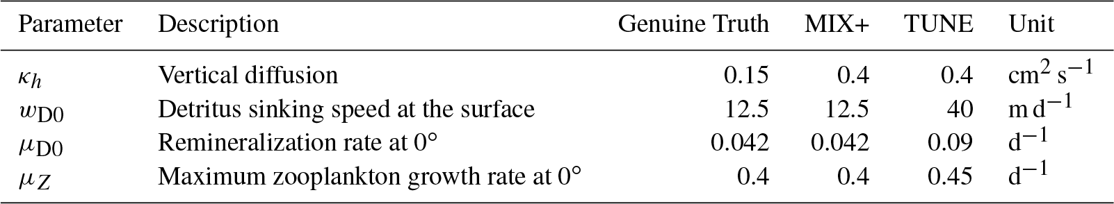
where DTR denotes the convergence (or divergence) of physical transports (sum of advection and isopycnal and diapycnal diffusion), and SRC denotes the source minus sink terms (such as differences between growth and mortality, air–sea fluxes, sinking). The biogeochemical module is described in detail in Keller et al. (2012) and Schmittner et al. (2008). Here, we present a choice of details relevant to those processes that we change (in the configuration TUNE, as described in Sect. 2.2). These processes are the sinking of detritus, the remineralization of detritus, and grazing by zooplankton. More specifically we apply changes to the following model parameters (see also Table 1): (1) the maximum grazing rate μZ, (2) the sinking speed of detritus wD0, and (3) the remineralization rate of detritus μD0. In the following we present the equations in which these model parameters are applied.
Phytoplankton growth is controlled by the availability of light and nutrients (here, nitrate, phosphate, and iron; the latter is parameterized by an iron mask based on monthly mean dissolved iron concentration outputs from the BLING model (Galbraith et al., 2010) rather than explicitly resolved). The simulated phytoplankton concentrations have a weak impact on sea surface temperatures as it is assumed that in the presence of phytoplankton more sunlight is absorption in the upper layer of the ocean model. Phytoplankton blooms are terminated by zooplankton grazing once essential nutrients are depleted. Zooplankton grazes on phytoplankton, diazotrophs, detritus, and other zooplankton (self-predation). Zooplankton growth is limited by a maximum zooplankton growth rate. This rate, , is dependent on temperature (T in units ∘C) and oxygen concentrations (O2 in units mmol m−3). In our parameter tuning experiment we change the value of the model parameter μZ in the equation
Both phytoplankton and zooplankton produce detritus that sinks to depth. This sinking speed, in combination with the remineralization rate, determines the depth range at which detritus is converted back into dissolved species (such as nitrate, phosphate, DIC) and stops sinking to the seafloor. The sinking speed of detritus, wD, increases linearly with depth:
where wD0 denotes the sinking speed at the surface and mW the derivative with respect to depth, and z is the effective vertical coordinate (positive downward). In our configuration TUNE we change the value of the model parameter wD0.
Remineralization of detritus returns the nitrogen (N) and phosphorus (P) content of detritus back to nitrate (NO3) and phosphate (PO4), consumes oxygen, and releases inorganic carbon. The rate of remineralization μD is both temperature dependent (T) and a function of ambient oxygen concentrations (it decreases by a factor of 5 in suboxic waters):
Tb is the e-folding temperature of biological rates (notation after Schmittner et al., 2008), and T and O2 are ambient temperature (∘C) and oxygen concentration (mmol O2 m−3), respectively. In one of our configurations we change the remineralization rate μD0, which sets the rate at 0 ∘C under oxygen-replete conditions.
2.2 Numerical experiments
We present results from numerical experiments with three different configurations of the numerical Earth system model UVic (see Table 2). For all three different configurations we apply both constant preindustrial atmospheric CO2 concentrations and increasing atmospheric CO2 emissions over time.
Table 1Model parameters explored for the three model configurations used in this study (see also Table 2). The Genuine Truth configuration is identical to the one introduced by Keller et al. (2012). MIX+ and TUNE are identical to the Genuine Truth except for the differences in parameter values listed here.
2.2.1 Model configurations
Table 2 lists the model configurations. The Genuine Truth configuration is identical to the reference simulation in Getzlaff and Dietze (2013) and has been developed and introduced by Keller et al. (2012). Note that this Genuine Truth model version by Keller et al. (2012) was modified (or tuned) such that the misfit to climatological observations of biogeochemical relevance, such as dissolved phosphate concentrations and phytoplankton (Garcia et al., 2010), is reduced relative to the original biogeochemical module from Schmittner et al. (2008). We compare this Genuine Truth to the model configurations with increased mixing, MIX+ and TUNE.
The first model modification, referred to as MIX+, is identical to the model version underlying the Genuine Truth, except for an increase in the vertical background diffusion from κh=0.15 up to 0.4 cm2 s−1 (see Tables 1 and 2). This choice is motivated by Kvale et al. (2017), who increased κh from 0.15 to 0.43 cm2 s−1 (in the same model) in order to compensate for a collapsed meridional overturning circulation when switching from one numerical advection scheme to another (to facilitate the design of an offline model version). Also, the regarded value is well within the range explored by Duteil and Oschlies (2011) with the same model.
Keller et al. (2012)(Getzlaff and Dietze, 2013)Table 2Configurations of the numerical Earth system model UVic (Weaver et al., 2007) used in this study.

TUNE is another twin to the Genuine Truth and identical to MIX+, except for changes to three biogeochemical model parameters: wD0, μD0, and μZ (see Table 1). The leading thought behind our changes relative to MIX+ is to mimic the behavior of the Genuine Truth configuration even though the vertical background diffusion is substantially different from the Genuine Truth. Or, in other words, changes to biogeochemical model parameters in TUNE are chosen such that the root mean square error (and with it the bias) in the simulated three-dimensional distribution of phosphate and phytoplankton concentrations between the Genuine Truth and MIX+ is compensated for. The procedure to achieve such a bias compensation is as follows. (1) We chose the three parameters somewhat arbitrarily, guessing that they are capable of reciprocally compensating for the effect of an increased vertical diffusivity. (2) We performed 48 spin-ups (see Sect. 2.2.2) with increased diffusivity and differing sets of values for the aforementioned biogeochemical model parameters. In these runs wD0 is spaced uniformly from 20 to 45 m d−1, μD0 from 0.07 to 0.09, and μZ from 0.4 to 0.45 (grid design; ). The idea behind this approach is to counteract the enhanced upwelling of nutrients by enhanced detritus export. Additionally, μD0 was increased to keep detritus concentrations on a reasonably low level. Note that prior to applying this concept to a 3-D model, it was tested in a simplified water column setup. (3) From this set of 48 we chose the configuration TUNE, which was “most similar” to the Genuine Truth (see Table 3). Following the rather generic workflow of biogeochemical model development we defined “similar to the Genuine Truth” as yielding a low volume-weighted root mean square error (RMSE) with respect to surface phytoplankton and global (3-D) oceanic phosphate concentrations (both values were averaged after unit conversion via a fixed Redfield ratio). This comparison between TUNE and the Genuine Truth was performed under preindustrial atmospheric CO2 concentrations (note that there is an ongoing discussion on misfit metrics that is beyond the scope of this paper; e.g., Evans, 2003; Löptien and Dietze, 2015). Please note that the parameter choice for TUNE that yields an even better bias compensation than the one we present in Table 1 may well exist and be found by using automated parameter optimization approaches such as suggested by Sauerland et al. (2009). Also, the bias might potentially be lowered when considering more biogeochemical model parameters. However, given the already remarkable similarity between TUNE and the Genuine Truth (as will be put forward in Sect. 3), we decided against the associated computational cost for the rather illustrative purpose of this study.
2.2.2 Spin-up procedure, historical model solution, and projections into the future
All numerical experiments presented in this study start from observed tracer distributions (Garcia et al., 2010). Each of the three model configurations (Genuine Truth, MIX+, and TUNE; Sect. 2.2.1) is then integrated under preindustrial atmospheric CO2 concentrations for 3000 years in order to reach quasi-equilibrated spun-up model states (e.g., Gupta et al., 2013) for all three configurations. The results (more specifically, the average of the last 10 years of the respective 3000-year spin-ups) of these three numerical experiments are dubbed historical model solutions because they are representative of the preindustrial world.
Subsequently, starting from the respective spun-up states of the three model configurations, so-called 1000-year-long drift runs are performed, wherein only the CO2 emissions (instead of concentrations) are prescribed, while the atmospheric CO2 content is allowed to vary in response to preindustrial emissions. After this drift phase virtual air–sea fluxes of biogeochemical species are also turned on (i.e., changes in DIC due to evaporation, precipitation, and runoff; Weaver et al., 2007). This procedure has proven to be efficient in switching from a prescribed atmospheric CO2 setup to an atmospheric emission-driven setup while keeping the spin-up times within reasonable bounds (also used in, e.g., Löptien and Dietze, 2017). Finally, we annex projections into the future by considering the years 1850–2100. From 2005 to 2100 we apply the emission scenario RCP8.5 (Riahi et al., 2011). Please note that differences among the three setups emerge during the transition phases. This model behavior is a reminder that, on the one hand, the state at which models are assessed matters, while on the other hand, there is no consensus on which state should be used for model assessment. In this study we follow the typical procedure as applied by, e.g., Reith et al. (2016).
In summary, we present six numerical experiments: a historical model solution and an RCP8.5 scenario for each of the three model configurations – Genuine Truth, MIX+, and TUNE.
In Sect. 3.1, we focus on the three historical model simulations (Genuine Truth, MIX+, and TUNE). This subsection illustrates reciprocal bias compensation. In Sect. 3.2, we present the results from the RCP8.5 scenario simulations. The aim of the latter is to explore the robustness of the reciprocal bias compensation under a typical global warming scenario.
3.1 Historical model solutions
The massive, severalfold increase in background diffusivity introduces surprisingly few differences in common ad hoc measures of the simulated ocean physics: the differences in sea surface temperature are very small in Fig. 1, and the relatively largest differences occur in the high latitudes, especially close to the ice edge. A similar picture evolves for sea surface salinity (Fig. 2): generally, differences in response to increased vertical mixing rates are small (Fig. 2c) with an exception in the Arctic where surface salinity increases by up to 1 PSU in response to increased vertical mixing rates. This is consistent with an increase in the meridional overturning circulation from 19 Sv in the Genuine Truth to 22 Sv in MIX+, which compensates for some of the net air–sea freshwater fluxes in the high latitudes (and thus increases sea surface salinities in these latitudes). Expressed in terms of a global mean difference, the Genuine Truth and MIX+ historical simulations differ by 0.03 K and 0.13 PSU only. Figure 3 supports the impression of similarity by showing that differences in the simulated zonally averaged net air–sea heat fluxes are within the range of measurement uncertainty in the field (e.g., Gulev et al., 2007). High values are restricted to very limited regions impacted by sea ice or deepwater formation.
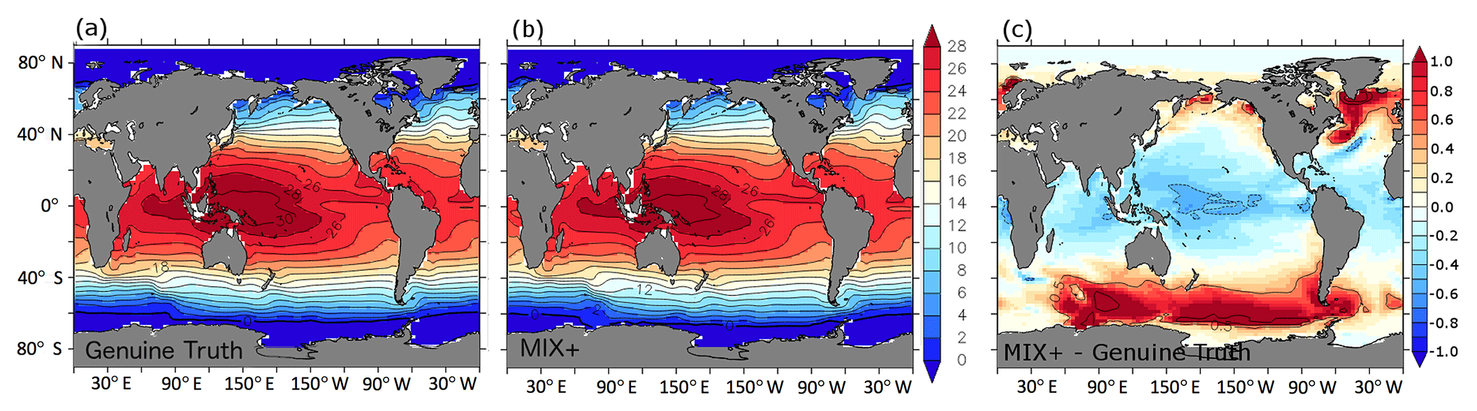
Figure 1Simulated sea surface temperature in degrees Celsius for the historical simulations (see Sect. 2.2.2). Panels (a) and (b) refer to results from the model configurations Genuine Truth and MIX+, respectively. MIX+ features an increased vertical background diffusivity relative to the Genuine Truth (see also Table 1). Panel (c) shows the difference between MIX+ and the Genuine Truth.
In contrast to the barely detectable changes in the physical ocean dynamics described above, conventional proxies for biogeochemical cycling turn out to be very sensitive to the change in vertical background diffusivity. The surface phosphate concentrations (compare panels (a) and (c) of Fig. 4) and surface phytoplankton concentrations (compare panels (a) and (c) of Fig. 5) showcase this amplified sensitivity of biogeochemical variables to changes in governing physics in a drastic way: while the increased vertical diffusion of cold abyssal waters from depth to the surface effects only minor changes to sea surface temperature and air–sea heat fluxes (as discussed above), it brings substantially more phosphate to the nutrient-depleted sunlit surface layer in which it drives a substantial increase in autotrophic production and the standing stock of phytoplankton. As a consequence, the cycling of phosphate in the upper thermocline accelerates. The export of particulate organic matter increases and the subsequent remineralization sharpens the vertical nutrient gradient at the base of the euphotic zone, which in turn increases diffusive nutrient fluxes to the sunlit surface layer. Among the overall net effects is the increased phosphate pool in the upper thermocline shown in Fig. 6 (except in the Southern Ocean where the combination of iron limitation, seasonal light limitation, and unique ventilation patterns overcomes the aforementioned effect). As concerns dissolved oxygen, the increase in vertical diffusivity has two opposing effects: on the one hand, the increased mixing ventilates the abyssal ocean by mixing oxygenated surface waters downward. On the other hand, the increased mixing accelerates biogeochemical cycling of organic matter (as described above) and thus, as a consequence of the associated accelerated remineralization of organic matter, increases the oxygen demand. Figure 7c reveals that the ventilating effect prevails in MIX+; i.e., the oceanic oxygen inventory rises in response to the higher diffusivity.
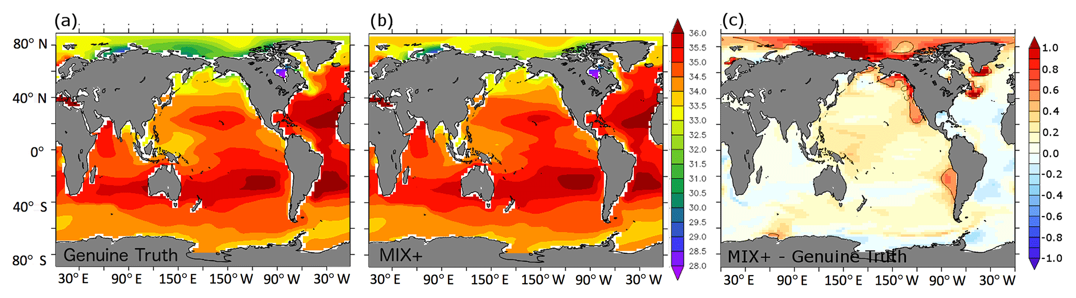
Figure 2Simulated sea surface salinity in practical salinity units (PSUs) for the historical simulations (see Sect. 2.2.2). Panels (a) and (b) refer to results from the model configurations Genuine Truth and MIX+, respectively. MIX+ features an increased vertical background diffusivity relative to the Genuine Truth (see Table 1). Panel (c) shows the difference between MIX+ and the Genuine Truth.
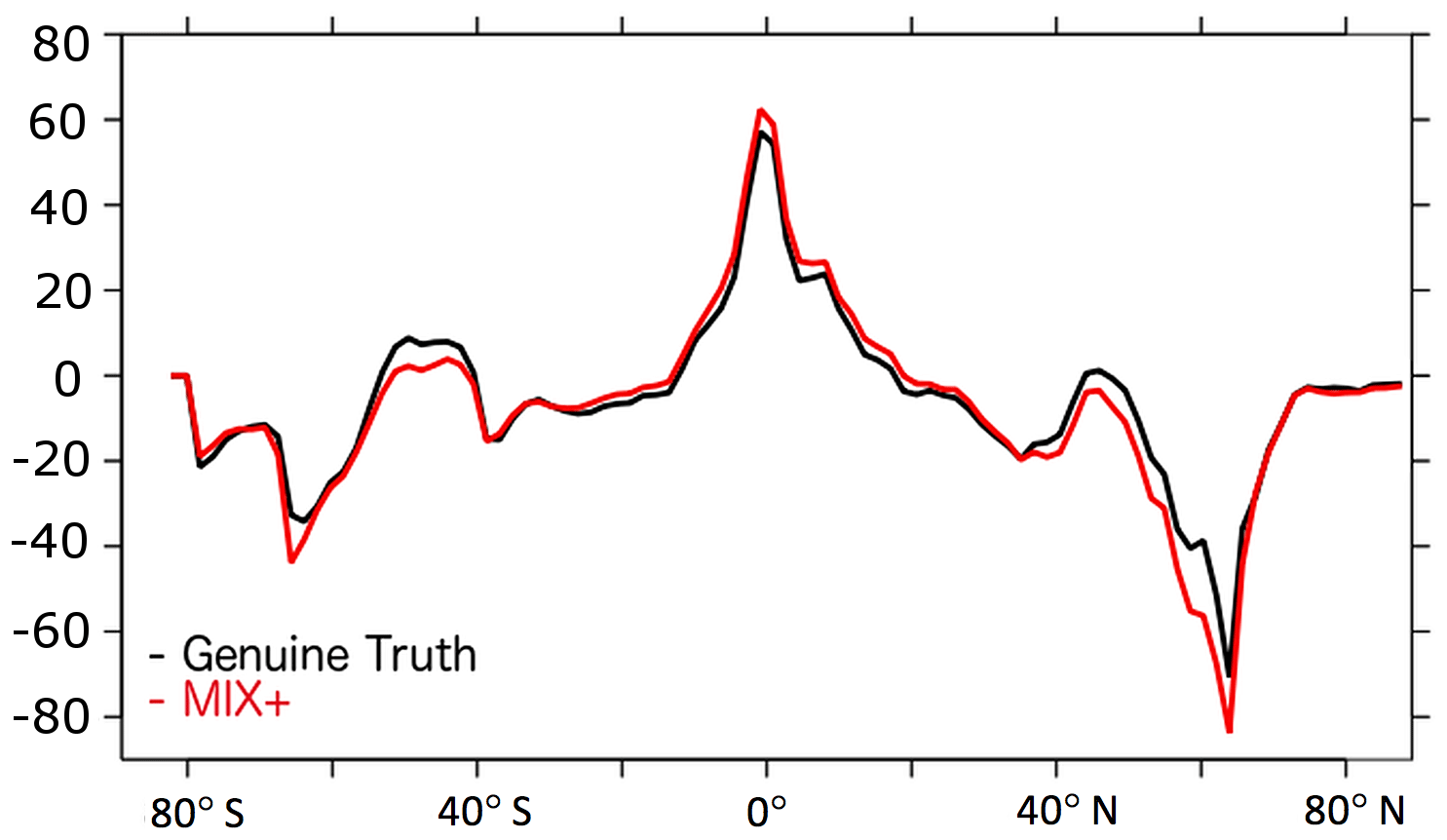
Figure 3Simulated zonally averaged net air–sea heat fluxes in watts per square meter (W m−2) for the historical simulations (see Sect. 2.2.2). Positive numbers denote ocean warming. The black and red lines refer to results from the model configurations Genuine Truth and MIX+, respectively.
The above results are in line with the intended model design (which mimics the typical workflow of Earth system model development): the Genuine Truth simulation represents a global set of (synthetic) observations. MIX+ is a physically biased model version of the Genuine Truth with, as illustrated above, drastic consequences for the simulated biogeochemical tracer distributions. The setup TUNE is an attempt to tweak (tune) the biogeochemistry in the deficient model MIX+ such that it resembles the Genuine Truth under historical conditions. Thus, in TUNE we compensate for the bias imposed by the physics via tuning the biogeochemistry. Under historical forcing, the physical ocean circulation is almost identical in TUNE and MIX+ (not shown). This low sensitivity might partly be due to the prescribed atmospheric CO2 concentrations in the historical simulations, since the feedback from changed biogeochemistry via oceanic carbon uptake to atmospheric CO2 and associated changes in air–sea heat fluxes is damped.
Table 3Misfits of historical model solutions relative to the Genuine Truth calculated as the volume-weighted root mean square error (RMSE) between respective numerical experiments. Note that only phosphate and phytoplankton concentrations were used to tune the model.
In terms of biogeochemistry, however, TUNE and MIX+ do differ considerably. Figures 4b and 5b show that the surface phosphate and phytoplankton concentrations simulated with TUNE are much more like the Genuine Truth than MIX+. Accordingly, the mean bias in surface phosphate decreases to 0.05 mmol P m−3 for the experiment TUNE relative to 0.27 mmol P m−3 in the simulation MIX+. Similarly, the bias in surface phytoplankton is reduced from 0.12 to −0.05 mmol N m−3 in TUNE. The similarity between the Genuine Truth and TUNE (in contrast to the difference between the Genuine Truth and MIX+) is not restricted to surface properties but extends to depth. For example, Fig. 6 shows that the zonally averaged phosphate concentrations of TUNE are much more similar to the Genuine Truth than is the case with MIX+. Further, Fig. 7b shows a similar behavior of the oceanic oxygen inventory. Expressed in numbers, the respective mean bias in TUNE is 12.99 mmol O2 m−3 relative to 30.08 mmol O2 m−3 in MIX+. A similar bias reduction in TUNE holds as well for the global extent of the simulated suboxic volume (not shown). The latter is remarkable since oxygen was not included in our metrics applied for the tuning process. Table 3 additionally contains a list of RMSEs relative to the Genuine Truth: e.g., the RMSE between global distributions of phosphate (phytoplankton) concentrations simulated with the Genuine Truth and MIX+ is 0.21 mmol P m−3 (0.1 mmol N m−3). By tweaking biogeochemical model parameters in simulation TUNE the RMSE is reduced by ≈40 % (down to 0.14 mmol P m−3 and 0.05 mmol N m−3; Table 3).
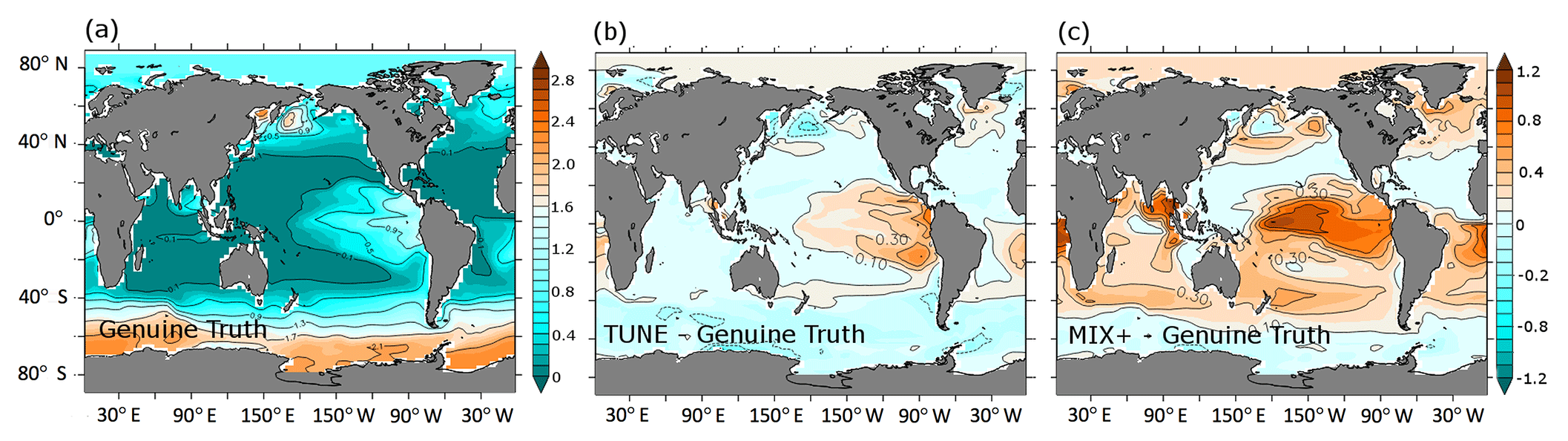
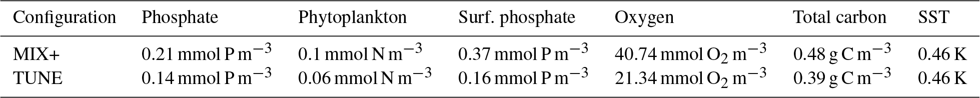
Figure 4Simulated surface phosphate concentrations in millimoles of phosphate per cubic meter (mmol P m−3) for the historical simulations (see Sect. 2.2.2). Panel (a) refers to results from the model configuration Genuine Truth. Panels (b) and (c) show the difference between the results from the model configurations TUNE and MIX+ and the Genuine Truth, respectively. MIX+ and TUNE feature increased vertical background diffusivity relative to the Genuine Truth. In addition, TUNE features retuned biogeochemical model parameters (see Table 1).
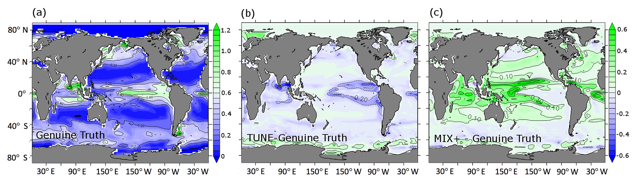
Figure 5Simulated phytoplankton concentrations in millimoles of nitrogen per cubic meter (mmol N m−3) for the historical simulations (see Sect. 2.2.2). Panel (a) refers to results from the model configuration Genuine Truth. Panels (b) and (c) show the difference between the results from the model configurations TUNE and MIX+ and the Genuine Truth, respectively. MIX+ and TUNE feature increased vertical background diffusivity relative to the Genuine Truth. In addition, TUNE features retuned biogeochemical model parameters (see Table 1).
3.2 Model projections into a warming future
All of our numerical configurations agree in that they feature a considerable sea surface temperature increase by the year 2100 when driven by the RCP8.5 greenhouse gas emission scenario (Riahi et al., 2011). The associated increase in radiative forcing warms the surface ocean and increases the stability of the water column (because relatively warmer and more buoyant water sits on top of cold abyssal water).
Expressed in terms of a global mean sea surface temperatures, the projected increase differs by up to 12 % depending on the underlying model configuration: the projected global mean temperature rise is 2.5, 2.2, and 2.3 K for the configurations Genuine Truth, TUNE, and MIX+, respectively. These differences among the experiments are consistent with the fact that (by construction) the simulations based on MIX+ and TUNE distribute heat over greater depth. Thus, their increased background diffusivity cools the surface (and warms the deep ocean) relative to the Genuine Truth. Consequentially, TUNE and MIX+ feature a stronger warming in the deep ocean than the Genuine Truth (the respective temperature increase is doubled below 1500 m of depth). This effect is somewhat offset in MIX+, which shows more temperature increase at the surface than TUNE, even though MIX+ and TUNE share the same physical model parameters. This is consistent with MIX+ featuring a phytoplankton standing stock that exceeds the standing stocks of both TUNE and the Genuine Truth by 150 %. This increased phytoplankton concentration absorbs more light at the surface and intensifies the surface warming.

Figure 6Differences between simulated meridionally averaged phosphate concentrations in millimoles of phosphate per cubic meter (mmol P m−3) for the historical simulations (see Sect. 2.2.2). Panels (a) and (b) refer to TUNE minus Genuine Truth and MIX+ minus Genuine Truth, respectively.
Figure 7(a) Simulated depth-averaged oxygen concentrations in millimoles of oxygen per cubic meter (mmol O2 m−3) for the historical simulation of the Genuine Truth. Panel (b) refers to the differences between TUNE and the Genuine Truth of simulated depth-averaged oxygen concentrations in units mmol O2 m−3 for the historical simulations (see Sect. 2.2.2). Panel (c) is identical to (b) but shows the difference to MIX+ instead of TUNE.
Regionally, the differences in projected sea surface temperatures (SSTs) can be much larger than in the global mean: Fig. 8 shows a comparison of sea surface temperature warming between TUNE and MIX+ relative to the Genuine Truth configuration in response to the RCP8.5 emission scenario. As expected, the comparisons to TUNE and MIX+ are very similar, but anomalies are somewhat more pronounced in TUNE. The differences between the TUNE and the Genuine Truth configuration exceed at maximum 1.8 K. The overall pattern is 0.2 to 0.5 K less warming in the Northern Hemisphere and 0.1 to 0.5 K more warming in the Southern Ocean in TUNE compared to the Genuine Truth. Hence, Southern Ocean SST warming in TUNE, in response to the increased greenhouse gas emissions, is stronger than in the Genuine Truth, even though the Genuine Truth overall warms more quickly than TUNE. We speculate that the increased background diffusivity in TUNE reduces the cooling effect of deep convection in the Southern Ocean by 2100 (relative to the Genuine Truth) because the abyssal waters (which the deep convection taps into) in TUNE have received more heat (relative to the Genuine Truth) prior to the year 1850. Also, the maximum overturning shows a stronger projected decline with increased vertical diffusivity.

Figure 8Comparison of sea surface temperature warming in response to RCP8.5 emissions. (a) The contours (both colored and labeled) denote the differences in simulated sea surface temperature anomalies between the years 2100 and 1850 in the projection based on the Genuine Truth setup in units of Kelvin. Panels (b) and (c) show the same differences for the projections based on TUNE and MIX+ relative to the Genuine Truth, respectively. Negative numbers indicate regions where the Genuine Truth warmed more than TUNE in the year 2100.
In terms of biogeochemistry, the similarity of model projections depends on the considered metric. For some biogeochemical tracers the reciprocal bias compensation (whereby an increase in diapycnal mixing is compensated for by changes to biogeochemical model parameters) is robust under global warming, while the historical similarities break for others. In Sect. 3.2.1 to 3.2.4 we illustrate the respective range. We start with a metric that is most robust and end with a metric with which the bias compensation breaks under the emission scenario.
3.2.1 Surface phytoplankton concentrations
Projections of phytoplankton are of interest because phytoplankton forms the base of the food chain and thereby exerts control on fisheries. The Genuine Truth simulation projects globally decreasing surface phytoplankton concentrations (see Fig. 9, left panel), corresponding to a global mean decrease of 7 % by 2100. This is consistent with the increased stability of the water column (effected by global warming), reducing the turbulent vertical mixing of nutrient-replete waters from depth to the nutrient-depleted sunlit surface ocean. In limited regions the projected changes can be opposed to the overall trend. These differences are most likely attributed to circulation changes (see Fig. 8). Examples of such regions are the Arctic, the equatorial Pacific, and the Southern Ocean.
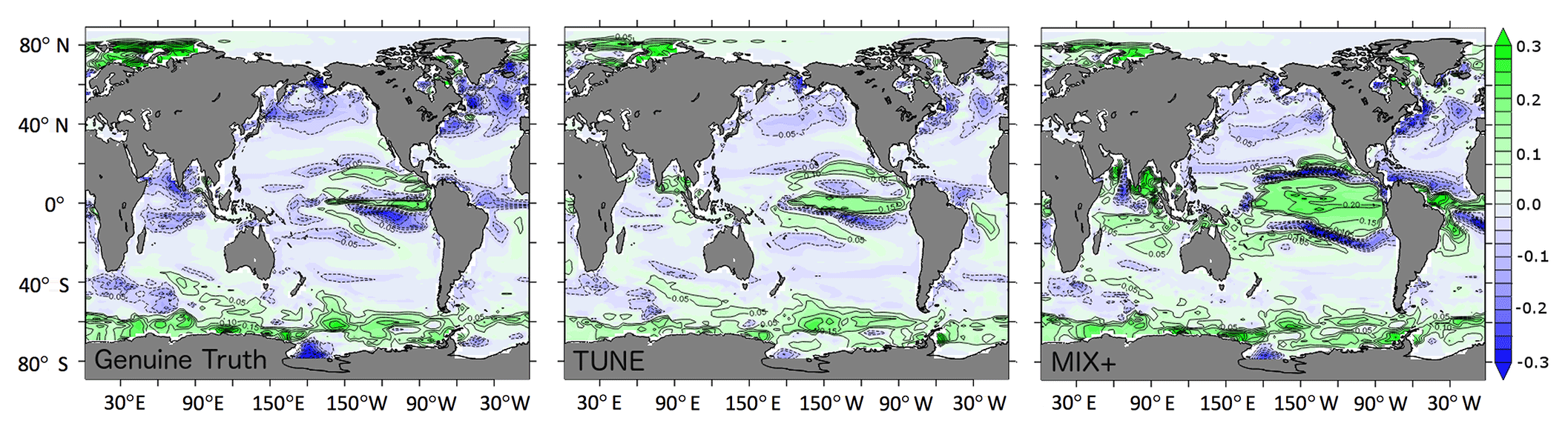
Figure 9Simulated changes in surface phytoplankton concentrations as a consequence of rising CO2 concentrations (emission scenario RCP8.5) calculated as the annual mean concentration difference between the years 2100 and 1850 (mmol N m−3).
The projection based on MIX+ differs substantially from the Genuine Truth in that it projects an overall increasing surface phytoplankton concentration (see Fig. 9). Most of this difference to the Genuine Truth is agglomerated in the Pacific Ocean, a region infamous for its nonlinear behavior (in our model; see also Sect. 3.2. in Löptien and Dietze, 2017). The projected phytoplankton change based on TUNE is very similar to the Genuine Truth (see Fig. 9, middle panel), corresponding to a globally averaged decrease of 8 % by 2100 – even though it shares the same biased physics with MIX+. This illustrates that for projected surface phytoplankton patterns the reciprocal bias compensation is (in our model) robust under the RCP8.5 scenario.
3.2.2 Surface phosphate concentrations
Projections of phosphate are of interest because phosphate is an essential nutrient that limits the growth of phytoplankton and the associated biotic export of organic matter to depth. In most state-of-the-art, global, coupled ocean circulation biogeochemical models, phosphate is the “base currency”; i.e., its cycling is directly (often linearly) related to the cycling of plankton and gases such as oxygen and CO2. The Genuine Truth simulation projects globally decreasing surface phosphate concentrations (see Fig. 10, left panel), corresponding to a global mean decrease of 17 % by 2100. As described above, this result is consistent with the increased stability of the water column that is effected by net air–sea heat fluxes (and associated buoyancy because warmer water is lighter than colder) caused by global warming. In the Southern Ocean, the processes at work are more complex. Here, the projected sea surface temperatures in the Genuine Truth simulation show alternating patterns of increasing and decreasing sea surface temperatures until the year 2100 (see Fig. 8). Downstream of regions where sea surface temperatures are reduced, more nutrients are mixed up to the surface in convective events and, simultaneously, surface mixed layers are increased. The latter leads to opposite effects compared to the above considerations on a global scale.

Figure 10Simulated changes in surface phosphate concentrations as a consequence of rising CO2 concentrations (emission scenario RCP8.5) calculated as the annual mean concentration difference between the years 2100 and 1850 (mmol P m−3).
The MIX+ projection is similar to the Genuine Truth as it projects that decreasing surface phosphate concentrations prevail globally (see Fig. 10, right panel). This decrease averages to 17 % globally by the year 2100. In the Southern Ocean, however, MIX+ differs substantially in that the alternating patches of increasing and decreasing surface phosphate concentrations apparent in the Genuine Truth are smoothed out (Fig. 10, compare left and right panel). We speculate that the absence of patches with strongly increasing surface phosphate indicates less-deep convection events. The latter is in line with the projected SSTs (Fig. 8).
The projection based on TUNE is generally very similar to the MIX+ projection: in this simulation decreasing surface phosphate concentrations also prevail globally (see Fig. 10, middle panel), corresponding to a globally averaged decrease of 17 % by 2100. In the Southern Ocean, however, TUNE is much more similar to MIX+ than the Genuine Truth. This illustrates that for projected surface phosphate patterns the reciprocal bias compensation is not very robust (especially locally, where circulation effects kick in) and some of the similarities apparent under historical conditions break under the RCP8.5 emission scenario.
3.2.3 Total oceanic carbon content
Projections of oceanic carbon content are of interest because the oceans currently take up a significant fraction of anthropogenic carbon emissions (of the order of 25 %; e.g., Takahashi et al., 2002). Therefore, changes in the capability of the ocean to sequester carbon away from the atmosphere in a warming future will directly affect the rate of global warming itself. This strong feedback is among the main drivers behind the development–inclusion of biochemical carbon modules in Earth system models that are used to assess the effects of climate change (and to develop mitigation strategies).
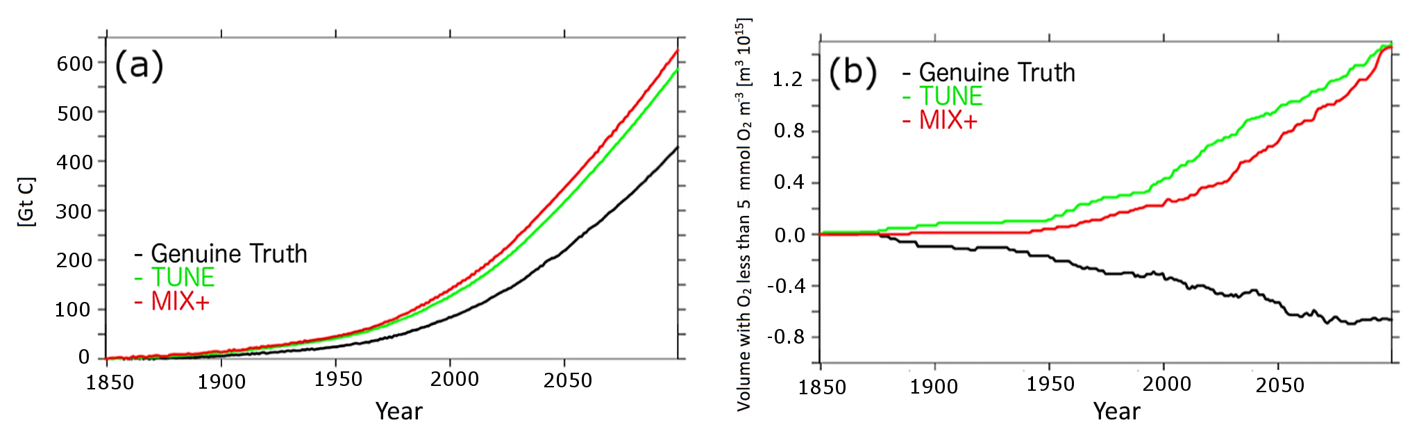
Figure 11(a) Differences in projected anomalous total carbon content of the ocean in response to rising CO2 concentrations (emission scenario RCP8.5; in units of gigatons of carbon). (b) Simulated temporal evolution of the volume of global suboxic waters (emission scenario RCP8.5).
Figure 11a shows that the reciprocal bias compensation is not robust when regarding the projected oceanic carbon content. In the historical model solutions, the simulated carbon content of the ocean varies by less than 0.6 % between the simulations. In the future projections, both MIX+ and TUNE propose to take up 200 Gt C more than the Genuine Truth by the year 2100. This difference refers to 32 % of the maximum projected change. In line with earlier studies, we presume that these strong differences must be attributed to differences in the solubility pump. Our results indicate that for oceanic carbon content, the reciprocal bias compensation is not robust once the boundary conditions strongly change.
3.2.4 Suboxic volume
Projections of suboxic volume are of interest because suboxia triggers denitrification and thus reduces the global availability of fixed nitrogen, an essential nutrient for all phytoplankton other than diazotrophs. Figure 11b shows that the suboxic volume, according to the Genuine Truth projection, decreases with global warming. A similar surprising behavior has been reported from other Earth system models (e.g., Gnanadesikan et al., 2011), which is surprising since it is counter to intuition because (1) warming reduces the solubility of oxygen, and (2) the increased stratification of the water column comes along with reduced ventilation; i.e., both of these processes directly associated with warming tend to reduce oceanic oxygen levels and thus promote suboxia.
MIX+ shows that an increased background diffusion can reverse the projected trend in suboxic volume. This is consistent with results from Gnanadesikan et al. (2011) and Getzlaff and Dietze (2013), highlighting the sensitivity of suboxic waters to the resolved and parameterized ocean physics.
The projection based on TUNE behaves like MIX+ in that it also shows a trend opposing the Genuine Truth. Remarkably, its trend is even more off relative to the Genuine Truth than the trend of MIX+. This illustrates that for suboxic volume the reciprocal bias compensation is not at all robust when the models are projected into the future.
We set out to explore reciprocal bias compensation in Earth system models in which deficiencies in the ocean circulation module are deliberately outweighed by tweaking the biogeochemical module. In the following, we will discuss the choice of our Earth system model (Sect. 4.1), the changes applied to the physical module (Sect. 4.2), and the changes applied to the biogeochemical module (Sect. 4.3). In Sect. 4.4 we will discuss the similarity between TUNE and Genuine Truth under historical forcing (and argue that we cannot decide based on ad hoc measures of typical present-day observations which setup is better suited to make reliable projections into a warming future). Section 4.5 closes this discussion by highlighting the differences between projections based on the model configurations TUNE and the Genuine Truth.
4.1 Choice of model framework
Our results are based on integrations of the UVic Earth system model (Keller et al., 2012). The model is relatively simple (i.e., it is an Earth system model of intermediate complexity – EMIC) and rather coarsely resolved (≈200 km) compared to the cutting-edge generation of IPPC-type atmosphere–ocean general circulation models (AOGCMs). Since EMICs and AOGCMs share very similar (or sometimes even identical) ocean circulation and pelagic biogeochemistry kernels, we speculate that our EMIC-based results are also applicable to IPCC-type AOGCMs. Accordingly, earlier findings from model intercomparison studies (e.g., Najjar et al., 2007) are consistent with our results. Even so, we wish to stress that our mixing parameter settings in MIX+ and TUNE are at the upper limit of proposed values and are chosen to cover the whole range.
We compare three configurations of UVic dubbed the Genuine Truth, MIX+, and TUNE. All setups are very similar (for the Genuine Truth even identical; see Sect. 2.2.1) to the Keller et al. (2012) configuration. This choice is motivated by the fact that this configuration is extensively used to assess the impact of geo-engineering options. Among recent studies are Partanen (2016), who explored the impacts of sea spray geo-engineering, Reith et al. (2016), who explored the effects of carbon sequestration by direct injection into the ocean, and Mengis et al. (2016), who assessed the effects of ocean albedo modification in the Arctic.
4.2 Choice of modification to background diffusivity
Two of our configurations (MIX+ and TUNE) feature an increased vertical diffusivity as the only change relative to the physical component of the original Keller et al. (2012) configuration (which we dubbed the Genuine Truth). The choice of changing the vertical background diffusivity is motivated by the fact that vertical diapycnal mixing is not well quantified in models or in the real ocean. What is known, though, is that diapycnal mixing is highly heterogenic both in time and space. Enhanced diffusivities up to 10 cm2 s−1 near the bottom have been observed over rough topography (Ledwell et al., 2000), while large-scale estimates derived from purposeful tracer release experiments in the subtropical North Atlantic yield values of 0.17±0.02 cm2 s−1 when considering a 2-year average (Ledwell et al., 1998). Even if the temporal and spacial variability were mapped out (which is not yet the case), the challenge is to transfer these numbers into a model parameterization that ensures realistic diffusive transports (of heat, salt, nutrients, etc.), which are defined as the product of the respective spacial (vertical) property gradient and diffusivity. Thus, using a vertical diffusivity that is averaged over time and space (as is inevitable in the current generation of models that apply a finite-difference discretization) is fraught with uncertainties. An additional source of uncertainty is implicit diffusion, a spurious and hard-to-quantify artifact (see Getzlaff et al., 2012) of the underlying numerical advection algorithm. To summarize: the uncertainty of the value of the vertical diffusion parameter of our physical model component is substantial and it cannot currently be well constrained by observations or experiments. Hence, we use the original diffusivity proposed for UVic and compare it to a value that was applied in the same model that uses a slightly different advection scheme but is otherwise identical. This model version with a changed advection scheme and increased diffusivity is used as the basis for the offline approach described by Kvale et al. (2017).
Using ad hoc measures, based on temperature and salinity, our change in diffusivity has a rather weak impact on physical tracers: only 0.03 K in terms of global sea surface temperature differences; in terms of meridional averaged heat fluxes, the differences are below 5 W m−2 from 50∘ S to 50∘ N, reaching 25 W m−2 at high latitudes.
The maximum meridional overturning circulation increases (as expected) with increased vertical diffusion and is 22 Sv in the reference simulation of MIX+ versus 19 Sv in the Genuine Truth. These numbers are broadly consistent with IPCC models: Marsland (2013) show values in the range 22–24 Sv for the Australian Community Climate and Earth System Simulator coupled CMIP5 model under preindustrial conditions. For the late twentieth century, Reintges et al. (2017) report an ensemble mean of a maximum overturning of 19 Sv in CMIP5 and 16 Sv in CMIP3 models. The spread among models in the late twentieth century has a range of 6.6–27.4 Sv in CMIP3 and 12.1–29.7 Sv in CMIP5 models, which is huge. Thus, the difference between the lowest and highest projected maximum overturning in CMIP5 models is almost as high as the present-day observational estimate (17.5 Sv based on the RAPID array at 26∘ N; Smeed et al., 2014).
4.3 Choice of changes to biogeochemical model parameters
One of our model configurations, TUNE, has both changed physics like MIX+ (described above) and changed biogeochemical parameter values chosen to reduce the misfit between this model and data (generated by Genuine Truth). To this end, μZ, μD, and wD0 have been changed by 12.5 %, ≈200 %, and 115 %, respectively. These changes are well within today's uncertainties, i.e., within the range of what is applied in other studies. For example, Kriest et al. (2017) assume that zooplankton mortality is uncertain within 4000 %, and the sinking speed at the surface in the Genuine Truth setup exceeds the value used by Ilyina et al. (2013) by 180 %. All parameter values considered in this study are well within the range used by Schartau (2003) in an automated parameter optimization study.
4.4 Similarity between the reciprocally bias-compensated couple
For the historical runs we showed in Sect. 3.1 that the simulations TUNE and the Genuine Truth are very similar to one another; i.e., the reciprocal bias compensation was effective. Given the close resemblance of temperature, salinity, air–sea heat fluxes, phosphate, phytoplankton, and oxygen in Figs. 1 to 7, we argue that both simulations, TUNE and the Genuine Truth, feature comparable misfits to observations for common model evaluation metrics. Since the Genuine Truth configuration is rated applicable to carry out geo-engineering studies (as outlined above), we conclude in turn that the configuration TUNE would be equally applicable to address today's pressing climate-related problems.
4.5 Ensuing uncertainties in response to RCP8.5
As outlined above, it is hard to argue based on a priori knowledge of the differences among their underlying model parameters which model configuration, the Genuine Truth or TUNE, is more realistic. Also, choosing the better model based on its performance in reproducing historical observations is difficult: the differences are rather small and the best choice will depend on the applied metric (or cost) to measure the misfit to the observations. It is disconcerting that the two configurations differ in what they project to come in response to the RCP8.5 emission scenario. The uncertainties in projected sea surface temperatures imposed by ocean mixing are locally substantial: for the Northern Hemisphere, we found differences of on average 0.5 K between the Genuine Truth and the simulation TUNE – a large value, particularly given that consensus has been reached on trying to keep global warming below 2 K. This finding, that vertical diffusion matters, is in line with earlier studies that stress the importance of the vertical diffusion coefficient for several physical properties of the ocean: e.g., Bryan (1987) pointed out that this parameter strongly impacts sensitivity towards wind forcing and thus the simulated large-scale meridional overturning.
In line with results from, e.g., Oschlies (2001) and Duteil and Oschlies (2011), we find that the uncertainty in background diffusivity also maps onto uncertainties in projected biogeochemical tracers. Striking examples, put forward in Sect. 3.2, are phytoplankton concentrations in the equatorial Pacific and suboxic volume (on which projections based on TUNE and the Genuine Truth do not agree, even on the sign of projected changes). The results for suboxic volume are consistent with findings by Cabré et al. (2015), who illustrate (in their Fig. 9) that the current generation of CMIP5 models does not agree on the sign of change either.
In terms of oceanic carbon content, the differences between TUNE and the Genuine Truth in projected future changes accumulate to 200 Gt of carbon in the year 2100. Again, this difference is substantial: expressed in terms of today's anthropogenic carbon emissions, the difference corresponds to 20 year's worth of anthropogenic emissions, which covers more than 40 % of the respective differences among CMIP5 models (Friedlingstein et al., 2014).
4.6 Model evaluation metrics
Our study stresses the urgent need to evaluate the mixing in ocean models carefully before projecting into the future. Our results are consistent with earlier findings within the Ocean Carbon-cycle Model Intercomparison Projects (OCIMIPs), which highlighted early on the importance of a realistic representation of physical ocean processes for modeling pelagic biogeochemistry (e.g., Doney et al., 2004). A definition of a suitable evaluation metric, apart from assessing relatively simple common measures such as temperature, salinity, and strength of the meridional overturning, is still not straightforward and today there is no consensus how to assess ocean models. It was suggested to also consider ventilation times (e.g., Matsumoto et al., 2004). Accordingly, additional inert chemical tracers (e.g., chlorofluorocarbons (CFC11, CFC12), SF6), allow for an extended model evaluation and are now required as standard output within CMIP6 (Orr et al., 2017). Still, many open questions and problems remain with such approaches. For example, the parameterized air–sea gas exchange induces large uncertainties (e.g., England et al, 1994). Furthermore, dating ranges of CFCs are not suitable to resolve the dynamics of the deep ocean, which recently led to an investigation of the use of 39Ar as an additional tracer (Ebser et al, 2018). The latter promising approach is currently under investigation. In summary, however, it still remains a pressing open question which misfit metrics ensure reliable projections. One major aim of the presented study is to remind us of these perpetual, often disregarded problems and to trigger related work. As a measure for diapycnal mixing in models we propose using the saturation state of noble gases, such as argon. Although noble gas concentrations are conservative tracers, their saturation states are not due to a nonlinear temperature and salinity dependence on their solubility (Bieri et al., 1966). In general, mixing of saturated water parcels affects temperature, salinity, and noble gas concentrations linearly and thus results in supersaturated argon concentrations.
We present results from two configurations of an Earth system model that feature a very similar behavior when driven with historical forcing but diverge drastically when used to project into our warming future based on the anthropogenic greenhouse gas emission scenario RCP8.5. The differences between the two configurations (dubbed the Genuine Truth and TUNE) are a modified vertical background diffusivity and changes applied to biogeochemical model parameters. The values of the biogeochemical model parameters were chosen to counteract the effects of the modified diffusivity. Note that the respective modification of the vertical diffusivity is within the range of what has recently been applied (see settings in Reith et al., 2016; Kvale et al., 2017). Likewise, the changes in biogeochemical model parameters are within the range of state-of-the-art model configurations (Schartau, 2003).
In terms of typical physical model assessment metrics (such as historical sea surface temperatures and meridional overturning estimates referring to currently applied assessment metrics such as in Kvale et al., 2017) and biogeochemical metrics (such as historical observations of phytoplankton and phosphate concentrations) neither of our two model configurations can be favored or discarded. The reason is that, first, our increase in vertical diffusivity has few effects on ad hoc measures of the ocean component in our model framework. Second, while the effect of our increased diffusivity substantially offsets generic biogeochemical assessment metrics (see configuration MIX+), we were able to compensate for a large part of the respective bias by changing biogeochemical model parameters. When driven with an RCP8.5 scenario, however, the similarity between our model configurations breaks for projections of societal relevance, such as the oceanic uptake of carbon or the dynamics of oxygen minimum zones. For carbon the projections accumulate a difference of 20 year's worth of today's anthropogenic emissions by the end of 2100. For the suboxic volume, not even the sign of forecasted changes coincides.
We conclude that an improved understanding of vertical diapycnal mixing in Earth system models alleviates the risk of reciprocal bias compensation by (wrongly) tweaking biogeochemical modules to a deficient physics, particularly when using ad hoc measures to assess the quality of the underlying ocean model. These results are consistent with earlier findings within the Ocean Carbon-cycle Model Intercomparison Projects (OCIMIPs) that highlighted the importance of a realistic representation of physical ocean processes for modeling pelagic biogeochemistry (e.g., Doney et al., 2004). Thus, an improved understanding of vertical diapycnal mixing can be expected to reduce ensuing uncertainties in climate projections considerably. Reverse reasoning suggests that an improved understanding of biogeochemistry can help to assess the realism of diapycnal mixing in Earth system models because (1) we found that some biogeochemical metrics are more sensitive to changes in mixing parameterization than typical physical metrics (such as overturning and temperature distributions), and (2) if the biogeochemical model formulations could be sufficiently constrained, then misfits between (more sensitive) biogeochemical metrics can be related back to deficiencies in the physical component of coupled ocean circulation biogeochemical models. With these findings, our study emphasizes the need to develop and routinely apply misfit metrics that take diapycnal mixing into account to obtain more reliable future projections.
The model code is archived at https://data.geomar.de/thredds/catalog/open_access/loeptien_dietze_2018_bg/catalog.html (last access: 1 May 2019). Since the use of the source code requires registration with the UVic model community (http://climate.uvic.ca/model/, last access: 14 February 2018, Eby, 2018), the respective file is password protected and available upon request. All required input files are downloadable under the above link.
The model output is archived at https://data.geomar.de/thredds/catalog/open_access/loeptien_dietze_2018_bg/catalog.html (last access: 1 May 2019).
Both authors were involved in the design of the work, in data analysis, in data interpretation, and in drafting the article.
The authors declare that they have no conflict of interest.
This work is a contribution of the project “Reduced Complexity Models” (supported by the Helmholtz Association of German Research Centres (HGF) – grant no. ZT-I-0010) and was additionally supported by the Deutsche Forschungsgemeinschaft (DFG) in the framework of the priority program “Antarctic Research with comparative investigations in Arctic ice areas” SPP 1158 by grant no. SCHN 762/5-1. We thank Anne Willem Omta and an anonymous reviewer for extremely detailed and helpful comments.
This paper was edited by Katja Fennel and reviewed by Anne Willem Omta and one anonymous referee.
Bieri, R. H., Koide, M., and Goldberg, E. D.: The noble gas contents of Pacific seawater, J. Geophys. Res., 71, 5243–5265, 1966. a
Bopp, L., Resplandy, L., Orr, J. C., Doney, S. C., Dunne, J. P., Gehlen, M., Halloran, P., Heinze, C., Ilyina, T., Séférian, R., Tjiputra, J., and Vichi, M.: Multiple stressors of ocean ecosystems in the 21st century: projections with CMIP5 models, Biogeosciences, 10, 6225–6245, https://doi.org/10.5194/bg-10-6225-2013, 2013. a
Bryan, F.: Parameter sensitivity of primitive equation ocean general circulation models, J. Phys. Oceanogr., 17, 970–985, 1987. a, b
Burchard, H.: Quantification of numerically induced mixing and dissipation in discretisations of shallow water equations, GEM-International, J. Geomath., 3, 51–65, https://doi.org/10.1016/j.ocemod.2007.10.003, 2012. a
Cabré, A., Marinov, I., Bernardello, R., and Bianchi, D.: Oxygen minimum zones in the tropical Pacific across CMIP5 models: mean state differences and climate change trends, Biogeosciences, 12, 5429–5454, https://doi.org/10.5194/bg-12-5429-2015, 2015. a
Dietze, H. and Löptien, U.: Revisiting nutrient trapping in global coupled biogeochemical ocean circulation models, Global Biogeochem. Cy., 27, 265–284, https://doi.org/10.1002/gbc.20029, 2013. a
Dietze, H. and Oschlies, A.: On the correlation between air-sea heat flux and abiotically induced oxygen exchange in a circulation model of the North Atlantic, J. Geophys. Res.-Oceans, 110, C09016, https://doi.org/10.1029/2004JC002453, 2005. a
Doney, S. C., Lindsay, K., Caldeira, K., Campin, J. M., Drange, H., Dutay, Follows, M., Gao, Y., Gnanadesikan, A., Gruber, N., Ishida, A., Joos, F., and Madec, G.: Evaluating global ocean carbon models: The importance of realistic physics. Global Biogeochem. Cy., 18, GB3017, https://doi.org/10.1029/2003GB002150, 2004. a, b
Duteil, O. and Oschlies, A.: Sensitivity of simulated extent and future evolution of marine suboxia to mixing intensity, Geophys. Res. Lett., 38, L06607, https://doi.org/10.1029/2011GL046877, 2011. a, b, c
Dutreuil, S., Bopp, L., and Tagliabue, A.: Impact of enhanced vertical mixing on marine biogeochemistry: lessons for geo-engineering and natural variability, Biogeosciences, 6, 901–912, https://doi.org/10.5194/bg-6-901-2009, 2009. a
Ebser, S., Kersting, A., Stöven, T., Feng, Z., Ringena, L., Schmidt, M., Tanhua, T., Aeschbach, W., and Oberthaler, M. K.: 39Ar dating with small samples resolves ocean ventilation, arXiv preprint arXiv:1807.11146, 2018. a
Eby, M.: Earth System Climate Model, available at: http://climate.uvic.ca/model/, last access: 14 February 2018. a
England, M. H., Garcon, V., and Minster, J. F.: Chlorofluorocarbon uptake in a world ocean model: 1. Sensitivity to the surface gas forcing, J. Geophys. Res.-Oceans, 99, 25215–25233, https://doi.org/10.1029/94JC02205, 1994. a
Evans, G. T.: Defining misfit between biogeochemical models and data sets, J. Mar. Syst., 40–41, 49–54, https://doi.org/10.1016/S0924-7963(03)00012-5, 2003. a
Fan, W. and Lv, X.: Data assimilation in a simple marine ecosystem model based on spatial biological parameterizations, Ecol. Model., 220, 1997–2008, https://doi.org/10.1016/j.ecolmodel.2009.04.050, 2009. a
Fasham, M. J. R., Evans, G. T., Kiefer, D. A., Creasey, M., and Leach, H.: The use of optimization techniques to model marine ecosystem dynamics at the JGOFS station at 47 degrees N 20 degrees W, P. Roy. Soc. Lond. B, 348, 203–209, 1995. a
Feng, Y., Koeve, W., Keller, D. P., and Oschlies, A.: Model-based Assessment of the CO2 Sequestration Potential of Coastal Ocean Alkalinization, Earth's Future, 5, 1252–1266, https://doi.org/10.1002/2017EF000659, 2017.
Fennel, K., Losch, M., Schröter, J., and Wenzel, M.: Testing a marine ecosystem model: sensitivity analysis and parameter optimization, J. Mar. Syst., 28, 450–63, https://doi.org/10.1016/S0924-7963(00)00083-X, 2001. a
Flynn, K. F.: Castles built on sand: dysfunctionality in plankton models and the inadequacy of dialogue between biologists and modellers, J. Plankton Res., 27, 1205–1210, https://doi.org/10.1093/plankt/fbi099, 2005.
Friedrichs, M. A. M., Hood, R. R., and Wiggert, J. D.: Ecosystem model complexity versus physical forcing: quantification of their relative impact with assimilated Arabian Sea data, Deep-Sea Res. Pt. II, 53, 576–600, https://doi.org/10.1016/j.dsr2.2006.01.026, 2006. a
Friedlingstein, P., Meinshausen, M., Arora, V. K., Jones, C. D., Anav, A., Liddicoat, S. K., and Knutti, R.: Uncertainties in CMIP5 climate projections due to carbon cycle feedbacks, J. Climate, 27, 511–526, https://doi.org/10.1175/JCLI-D-12-00579.1, 2014. a, b
Garcia, H. E., Locarnini, R. A., Boyer, T. P., Antonov, J. I., Zweng, M. M., Baranova, O. K., and Johnson, D. R.: World Ocean Atlas 2009, Volume 4: Nutrients (phosphate, nitrate, silicate), edited by: Levitus, S., NOAA Atlas NESDIS 71, U.S. Government Printing Off, 2010. a, b, c
Galbraith, E. D., Gnanadesikan, A., Dunne, J. P., and Hiscock, M. R.: Regional impacts of iron-light colimitation in a global biogeochemical model, Biogeosciences, 7, 1043–1064, https://doi.org/10.5194/bg-7-1043-2010, 2010. a
Getzlaff, J. and Dietze, H.: Effects of increased isopycnal diffusivity mimicking the unresolved equatorial intermediate current system in an earth system climate model, Geophys. Res. Lett., 40, 2166–2170, https://doi.org/10.1002/grl.50419, 2013. a, b, c
Getzlaff, J., Nurser, G., and Oschlies, A.: Diagnostics of diapycnal diffusivity in z-level ocean models part I: 1-Dimensional case studies, Ocean Model., 35, 173–186, https://doi.org/10.1016/j.ocemod.2010.07.004, 2010. a
Getzlaff, J., Nurser, G., and Oschlies, A.: Diagnostics of diapycnal diffusion in z-level ocean models. Part II: 3-dimensional OGCM, Ocean Model., 45, 27–36, https://doi.org/10.1016/j.ocemod.2011.11.006, 2012. a, b
Getzlaff, J., Dietze, H., and Oschlies, A.: Simulated effects of southern hemispheric wind changes on the Pacific oxygen minimum zone, Geophys. Res. Lett., 43, 728–734, https://doi.org/10.1002/2015GL066841, 2016.
Gnanadesikan, A., Dunne, J. P., and John, J.: Understanding why the volume of suboxic waters does not increase over centuries of global warming in an Earth System Model, Biogeosciences, 9, 1159–1172, https://doi.org/10.5194/bg-9-1159-2012, 2012. a, b
Gulev, S., Jung, T., and Ruprecht, E.: Estimation of the impact of sampling errors in the VOS observations on air-sea fluxes. Part I: Uncertainties in climate means, J. Climate, 20, 279–301, https://doi.org/10.1175/JCLI4010.1, 2007. a
Gupta, A. S., Jourdain, N. C., Brown, J. N., and Monselesan, D.: Climate drift in the CMIP5 models, J. Climate, 26, 8597–8615, https://doi.org/10.1175/JCLI-D-12-00521.1, 2013. a
Hemmings, J. C. P. and Challenor, P. G.: Addressing the impact of environmental uncertainty in plankton model calibration with a dedicated software system: the Marine Model Optimization Testbed (MarMOT 1.1 alpha), Geosci. Model Dev., 5, 471–498, https://doi.org/10.5194/gmd-5-471-2012, 2012. a
Ilicak, M., Adcroft, A. J., Griffies, S. M., and Hallberg, R. W.: Spurious dianeutral mixing and the role of momentum closure, Ocean Model., 45, 37–58, https://doi.org/10.1016/j.ocemod.2011.10.003, 2012. a
Ilyina, T., Six, K. D., Segschneider, J., Maier-Reimer, E., Li, H., and Nunez-Riboni, I.: Global ocean biogeochemistry model HAMOCC: Model architecture and performance as component of the MPI-Earth system model in different CMIP5 experimental realizations, J. Adv. Model. Earth Sy., 5, 287–315, https://doi.org/10.1029/2012MS000178, 2013. a, b
Keller, D. P., Oschlies, A., and Eby, M.: A new marine ecosystem model for the University of Victoria Earth System Climate Model, Geosci. Model Dev., 5, 1195–1220, https://doi.org/10.5194/gmd-5-1195-2012, 2012. a, b, c, d, e, f, g, h, i, j, k, l
Keller, D. P., Feng, E. Y., and Oschlies, A.: Potential climate engineering effectiveness and side effects during a high carbon dioxide-emission scenario, Nat. Commun., 5, 3304, https://doi.org/10.1038/ncomms4304, 2014. a
Kriest, I., Khatiwala, S., and Oschlies, A.: Towards an assessment of simple global marine biogeochemical models of different complexity, Prog. Oceanogr., 86, 337–360, https://doi.org/10.1016/j.pocean.2010.05.002, 2010. a
Kriest, I., Sauerland, V., Khatiwala, S., Srivastav, A., and Oschlies, A.: Calibrating a global three-dimensional biogeochemical ocean model (MOPS-1.0), Geosci. Model Dev., 10, 127–154, https://doi.org/10.5194/gmd-10-127-2017, 2017. a
Kvale, K. F., Khatiwala, S., Dietze, H., Kriest, I., and Oschlies, A.: Evaluation of the transport matrix method for simulation of ocean biogeochemical tracers, Geosci. Model Dev., 10, 2425–2445, https://doi.org/10.5194/gmd-10-2425-2017, 2017. a, b, c, d
Large, W. G., Danabasoglu, G., McWilliams, J. C., Gent, P. R., and Bryan, F. O.: Equatorial circulation of a global ocean climate model with anisotropic horizontal viscosity, J. Phys. Oceanogr., 31, 518–536, https://doi.org/10.1175/1520-0485(2001)031<0518:ECOAGO>2.0.CO;2, 2001. a
Lawson, L. M., Hofmann, E. E., and Spitz, Y. H.: Time series sampling and data assimilation in a simple marine ecosystem model, Deep-Sea Res. Pt. II, 43, 625–651, https://doi.org/10.1016/0967-0645(95)00096-8, 1996. a
Ledwell, J. R., Watson, A. J. and Law, C. S.: Mixing of a tracer in the pycnocline, J. Geophys. Res., 103, 499–529, https://doi.org/10.1029/98JC01738, 1998. a, b
Ledwell, J. R., Montgomery, E. T. Polzin, K. L., Laurent, L. S. Schmitt, R. W., and Toole, J. M.: Evidence for enhanced mixing over rough topography in the abyssal ocean, Nature, 403, 6766, https://doi.org/10.1038/35003164, 2000. a
Lemarié, F., Debreu, L., Shchepetkin, A. F., and McWilliams, J. C.: On the stability and accuracy of the harmonic and biharmonic isoneutral mixing operators in ocean models, Ocean Model., 52–53, 9–35, https://doi.org/10.1016/j.ocemod.2012.04.007, 2012. a
Löptien, U. and Dietze, H.: Constraining parameters in marine pelagic ecosystem models – is it actually feasible with typical observations of standing stocks?, Ocean Sci., 11, 573–590, https://doi.org/10.5194/os-11-573-2015, 2015. a, b
Löptien, U. and Dietze, H.: Effects of parameter indeterminacy in pelagic biogeochemical modules of Earth System Models on projections into a warming future: The scale of the problem, Global Biogeochem. Cy., 31, 1155–1172, https://doi.org/10.1002/2017GB005690, 2017. a, b, c
Matsumoto, K., Sarmiento, J. L., Key, R. M., Aumont, O., Bullister, J. L., Caldeira, K., Campin, J. M., Doney, S. C., Drange, H., Dutay, J. C., Follows, M., Gao, Y., Gnanadesikan, A., Gruber, N., Ishida, A., Joos, F., Lindsay, K., Maier-Reimer, E.,Marshall, J. C., Matear, R. J., Monfray, P., Mouchet, A., Najjar, R., Plattner, G. K., Schlitzer, R., Slater, R., Swathi, P. S., Totterdell, I. J., Weirig, M. F., Yamanaka, Y., Yool A., and Orr, J. C.: Evaluation of ocean carbon cycle models with data-based metrics, Geophys. Res. Lett., 31, L07303, https://doi.org/10.1029/2003GL018970, 2004. a
Marsland, S. J., Bi, D., Uotila, P., Fiedler, R., Griffies, S. M., Lorbacher, K., O'Farrell, S., Sullivan, A., Uhe, P., Zhou, X., and Hirst, A. C.: Evaluation of ACCESS climate model ocean diagnostics in CMIP5 simulations, Aust. Meteorol. Ocean., 63, 101–119, https://doi.org/10.22499/2.6301.004, 2013. a
Matear, R. J.: Parameter optimization and analysis of ecosystem models using simulated annealing: a case study at station P, J. Mar. Res., 53, 571–607, https://doi.org/10.1357/0022240953213098, 1995. a, b
Mathieu, P.-P. and Deleersnijder, E.: What is wrong with isopycnal diffusion in world ocean models?, Applied Mathmatical Modelling, 22, 367–378, https://doi.org/10.1016/S0307-904X(98)10008-2, 1998. a
Matthews, H. D., Cao, L., and Caldeira, K.: Sensitivity of ocean acidification to geoengineered climate stabilization, Geophys. Res. Lett. 36, 10706, https://doi.org/10.1029/2009GL037488, 2009. a
Mengis, N., Martin, T., Keller, D. P., and Oschlies, A.: Assessing climate impacts and risks of ocean albedo modification in the Arctic, J. Geophys. Res.-Oceans, 121, 3044–3057, https://doi.org/10.1002/2015JC011433, 2016. a
Najjar, R. G., Jin, X., Louanchi, F., Aumont, O., Caldeira, K., Doney, S. C., Dutay, J. C., Follows, M., Gruber, N., Joos, F., Lindsay, K., Maier-Reimer, E., Matear, R. J., Matsumoto, K., Monfray, P., Mouchet, A., Orr, J. C., Plattner, G. K., Sarmiento, J., Schlitzer, R., Weirig, M. F., Yamanaka, Y., and Yool, A.: Impact of circulation on export production, dissolved organic matter and dissolved oxygen in the ocean: Results from OCMIP-2, Global Biogeochem. Cy., 21, GB3007, https://doi.org/10.1029/2006GB002857, 2007. a
Orr, J. C., Najjar, R. G., Aumont, O., Bopp, L., Bullister, J. L., Danabasoglu, G., Doney, S. C., Dunne, J. P., Dutay, J.-C., Graven, H., Griffies, S. M., John, J. G., Joos, F., Levin, I., Lindsay, K., Matear, R. J., McKinley, G. A., Mouchet, A., Oschlies, A., Romanou, A., Schlitzer, R., Tagliabue, A., Tanhua, T., and Yool, A.: Biogeochemical protocols and diagnostics for the CMIP6 Ocean Model Intercomparison Project (OMIP), Geosci. Model Dev., 10, 2169–2199, https://doi.org/10.5194/gmd-10-2169-2017, 2017. a
Oschlies, A.: Model-derived estimates of new production: New results point towards lower values, Deep-Sea Res. Pt. II, 48, 2173–2197, https://doi.org/10.1016/S0967-0645(00)00184-3, 2001. a, b
Oschlies, A., Pahlow, M., Yool, A., and Matear, R. M.: Climate engineering by artificial ocean upwelling: channelling the sorcerer's apprentice, Geophys. Res. Lett., 37, 1–5, https://doi.org/10.1029/2009GL041961, 2010. a, b
Osborn, T. R. and Cox, C. S.: Oceanic fine structure, Geophys. Fluid Dynam., 3, 321–345, 1971.
Pacanowski, R. C.: MOM 2 documentation, user's guide and reference manual. GFDL Ocean Group Tech. Rep, 3, 232 pp., 1995. a
Partanen, A. I., Keller, D. P., Korhonen, H., and Matthews, H. D.: Impacts of sea spray geoengineering on ocean biogeochemistry, Geophys. Res. Lett., 43, 7600–7608, https://doi.org/10.1002/2016GL070111, 2016. a
Prange, M., Lohmann, G., and Paul, A.: Influence of vertical mixing on the thermohaline hysteresis: Analyses of an OGCM, J. Phys. Oceanogr., 33, 1707–1721, https://doi.org/10.1175/2389.1, 2003. a
Reintges, A., Martin, T., Latif, M., and Keenlyside, N. S.: Uncertainty in twenty-first century projections of the Atlantic Meridional Overturning Circulation in CMIP3 and CMIP5 models, Clim. Dynam., 49, 1495–1511, https://doi.org/10.1007/s00382-016-3180-x, 2017. a
Reith, F., Keller, D. P., and Oschlies, A.: Revisiting ocean carbon sequestration by direct injection: a global carbon budget perspective, Earth Syst. Dynam., 7, 797–812, https://doi.org/10.5194/esd-7-797-2016, 2016. a, b, c, d
Riahi, K., Rao, S., Krey, V., Cho, C., Chirkov, V., Fischer, G., Kindermann, G., Nakicenovic, N., and Rafaj, P.: RCP 8.5 – A scenario of comparatively high greenhouse gas emissions, Clim. Change, 109, 33–57, https://doi.org/10.1007/s10584-011-0149-y, 2011. a, b
Rückelt, J., Sauerland, V., Slawig, T., Srivastav, B., Ward, C., and Patvardhan, C.: Parameter optimization and uncertainty analysis in a model of oceanic CO2 uptake using a hybrid algorithm and algorithmic differentiation, Nonlinear Anal.-Real, 11, 3993–4009, https://doi.org/10.1016/j.nonrwa.2010.03.006, 2010. a
Sauerland, V., Löptien, U., Leonhard, C., Oschlies, A., and Srivastav, A.: Error assessment of biogeochemical models by lower bound methods (NOMMA-1.0), Geosci. Model Dev., 11, 1181–1198, https://doi.org/10.5194/gmd-11-1181-2018, 2018. a
Schartau, M.: Simultaneous data-based optimization of a 1D-ecosystem model at three locations in the North Atlantic Ocean: Part I – method and parameter estimates, J. Mar. Res., 62, 765–793, https://doi.org/10.1357/002224003322981147, 2003. a, b, c
Schartau, M., Oschlies, A., and Willebrand, J.: Parameter estimates of a zero-dimensional ecosystem model applying the adjoint method, Deep-Sea Res. Pt. II, 48, 1769–1800, https://doi.org/10.1016/S0967-0645(00)00161-2, 2001. a
Smeed, D. A., McCarthy, G. D., Cunningham, S. A., Frajka-Williams, E., Rayner, D., Johns, W. E., Meinen, C. S., Baringer, M. O., Moat, B. I., Duchez, A., and Bryden, H. L.: Observed decline of the Atlantic meridional overturning circulation 2004–2012, Ocean Sci., 10, 29–38, https://doi.org/10.5194/os-10-29-2014, 2014. a
Schmittner, A., Oschlies, A., Matthews, H. D., and Galbraith, E. D.: Future changes in climate, ocean circulation, ecosystems, and biogeochemical cycling simulated for a business-as-usual CO2 emission scenario until year 4000 AD, Global Biogeochem. Cy., 22, GB1013, https://doi.org/10.1029/2007GB002953, 2008. a, b, c
Sinha, B., Buitenhuis, E. T., Quéré, C. L., and Anderson, T. R.: Comparison of the emergent behavior of a complex ecosystem model in ocean general circulation models, Prog. Oceanogr., 84, 204–224, https://doi.org/10.1016/j.pocean.2009.10.003, 2010. a
Simmons, H. L., Jayne, S. R., St. Laurent, L. C., and Weaver, A. J.: Tidally driven mixing in a numerical model of the ocean general circulation, Ocean Model., 6, 245–263, 2004. a
Somes, C. J., Schmittner, A., Galbraith, E. D., Lehmann, M. F., Altabet, M. A., Montoya, J. P., Letelier, R. M., Mix, A. C., Bourbonnais, A., and Eby, M.: Simulating the global distribution of nitrogen isotopes in the ocean, Global Biogeochem. Cy., 24, GB4019, https://doi.org/10.1029/2009GB003767, 2010. a
Spitz, Y. H., Moisan, J. R., Abbott, M. R., and Richman, J. G.: Data assimilation and a pelagic ecosystem model: parameterization using time series observations, J. Mar. Syst., 16, 51–68, https://doi.org/10.1016/S0924-7963(97)00099-7, 1998. a
Takahashi, T., Sutherland, S. C., Sweeney, C., Poisson, A., Metzl, N., Tilbrook, B., Bates, N., Wanninkhof, R., Feely, R. A., Sabine, C., Olafsson, J., and Nojiri, Y.: Global sea-air CO2 flux based on climatological surface ocean pCO2, and seasonal biological and temperature effects, Deep-Sea Res. Pt. II, 49, 1601–1622, https://doi.org/10.1016/S0967-0645(02)00003-6, 2002. a
Ward, B. A., Friedrichs, M. A. M., Anderson, T. A., and Oschlies, A.: Parameter optimisation techniques and the problem of underdetermination in marine biogeochemical models, J. Mar. Syst., 81, 34–43, https://doi.org/10.1016/j.jmarsys.2009.12.005, 2010. a
Weaver, A. J., Eby, M., Wiebe, E. C., Bitz, C. M., Duffy, P. B., Ewen, T. L., Fanning, A. F., Holland, M. M., MacFadyen, A., Matthews, H. D., Meissner, K. J., Saenko, O., Schmittner, A., Wang, H., and Yoshimori, M.: The UVic Earth System Climate Model: Model description, climatology, and applications to past, present and future climates, Atmos.-Ocean, 39, 361–428, https://doi.org/10.1080/07055900.2001.9649686, 2001. a, b
Weaver, A. J., Zickfeld, K., Montenegro, A., and Eby, M.: Long term climate implications of 2050 emission reduction targets, Geophys. Res. Lett., 34, L19703, https://doi.org/10.1029/2007GL031018, 2007. a, b
Williamson, P., Wallace, D. W. R., Law, C. S., Boyd, P. W., Collos, Y., Croot, P., Denman, K., Riebesell, U., Takeda, S., and Vivian, C.: Ocean fertilization for geoengineering: a review of effectiveness, environmental impacts and emerging governance, Process Saf. Environ., 90, 475–488, https://doi.org/10.1016/j.psep.2012.10.007, 2012. a
Xiao, Y. and Friedrichs, M. A. M.: The assimilation of satellite-derived data into a one-dimensional lower trophic level marine ecosystem model, J. Geophys. Res.-Oceans, 119, 2691–2712, https://doi.org/10.1002/2013JC009433, 2014. a
Yool, A., Shepherd, J. G., Bryden, H. L., and Oschlies, A.: Low efficiency of nutrient translocation for enhancing oceanic uptake of carbon dioxide, J. Geophys. Res., 114, 1–13, https://doi.org/10.1029/2008JC004792, 2009. a