the Creative Commons Attribution 4.0 License.
the Creative Commons Attribution 4.0 License.
 | 26 Apr 2019
Assessment of time of emergence of anthropogenic deoxygenation and warming: insights from a CESM simulation from 850 to 2100 CE
Juliette Mignot
Fortunat Joos
Marine deoxygenation and anthropogenic ocean warming are observed and projected to intensify in the future. These changes potentially impact the functions and services of marine ecosystems. A key question is whether marine ecosystems are already or will soon be exposed to environmental conditions not experienced during the last millennium. Using a forced simulation with the Community Earth System Model (CESM) over the period 850 to 2100, we find that anthropogenic deoxygenation and warming in the thermocline exceeded natural variability in, respectively, 60 % and 90 % of total ocean area. Control simulations are typically used to estimate the pre-industrial variability level. However, the natural variability of oxygen (O2) and temperature (T) inferred from the last millennium period is systematically larger than the internal variability simulated in the corresponding control simulation. This renders natural variability from control simulations to be biased towards low estimates. Here, natural variability is assessed from the last millennium period (850–1800 CE), thus considering the response to forcing from explosive volcanic eruptions, solar irradiance and greenhouse gases in addition to internal, chaotic variability. Results suggest that in the tropical thermocline, where biological and solubility-driven O2 changes counteract each other, anthropogenic changes in apparent oxygen utilisation (AOU) and in O2 solubility (O2,sol) are detectable earlier than O2 changes. Both natural variability and change in AOU are predominantly driven by variations in circulation with a smaller role for productivity. By the end of the 21st century, ventilation becomes more vigorous in the tropical thermocline, whereas ideal age in deep waters increases by more than 200 years relative to the pre-industrial period. Different methodological choices are compared and the time for an anthropogenic signal to emerge (ToE) is earlier in many thermocline regions when using variability from a shorter period, from the control simulation or estimates from the industrial period instead of the variability from the last millennium. Our results highlight that published methods may lead to deviations in ToE estimates, calling for a careful quantification of variability. They also highlight that realised anthropogenic change exceeds natural variations in many regions.


Oceanic oxygen O2 concentrations have been observed to decrease over the past 50 years (e.g. Stramma et al., 2008; Helm et al., 2011; Ito et al., 2017; Schmidtko et al., 2017) and are projected to further decline under anthropogenic climate change (Sarmiento et al., 1998; Plattner et al., 2001; Keeling and Garcia, 2002; Shaffer et al., 2009; Cocco et al., 2013; Battaglia and Joos, 2018). This deoxygenation, in combination with other stressors (Bopp et al., 2013; Cocco et al., 2013), such as ocean warming (IPCC, 2013), poses major risks for the function of marine ecosystems and the services they provide (Gattuso et al., 2015; Mislan et al., 2017; Breitburg et al., 2018). The natural climate variability of the recent past provides a range of “familiar” climate conditions to which many ecological and socio-economic systems are adapted. Forcing environmental conditions outside the bounds of recent natural variability may trigger adverse impacts (Pörtner et al., 2014). It is still an open question to which extent marine species and ecosystems are already confronted with “unfamiliar” environmental and climatic conditions not encountered during the last millennium. A difficulty arises from the need to quantify natural variability that stems both from the partly chaotic internal variability of the climate system (Lorenz, 1963; Hasselmann, 1976) and from natural external forcing factors including variations in solar energy output and explosive volcanic eruptions (e.g. Jungclaus et al., 2017). Studies that address the natural variability of marine O2 and temperature during the recent millennium and that compare this variability with anthropogenic change are missing.
The time of emergence (ToE) is an established metric to estimate when a forced anthropogenic change or “signal” exceeds variability or “noise” (Christensen et al., 2007; Hawkins and Sutton, 2012). ToE is the point in time when the anthropogenic changes becomes larger than natural variability. ToE has been estimated for physical climate variables (e.g. Christensen et al., 2007; Hawkins and Sutton, 2012; Mahlstein et al., 2013; Deser et al., 2014; Frame et al., 2017), land carbon stocks and fluxes (Lombardozzi et al., 2014) and marine properties including ocean acidification impacts and alkalinity (Ilyina et al., 2009; Friedrich et al., 2012; Ilyina and Zeebe, 2012; Hauri et al., 2013), sea surface temperature, pH, CO2 partial pressure and dissolved inorganic carbon (Christian, 2014; Keller et al., 2014), marine biological productivity, biological export fluxes, surface chlorophyll and surface nitrate (Henson et al., 2016) and air-to-sea carbon fluxes (McKinley et al., 2016).
Studies that address the ToE for temperature in the thermocline are nevertheless still missing. This is a gap as the observed and projected warming in the thermocline affects the physiology of fish and their habitat distribution in addition to changes in O2 (Pörtner et al., 2014). A limited number of studies addressed the ToE for O2 in the thermocline, often in combination for other tracers (Rodgers et al., 2015; Frölicher et al., 2016; Henson et al., 2016, 2017; Long et al., 2016). The results demonstrate a wide range of ToE associated with the range of different methods used.
The method applied for estimating ToE depends on the scientific questions. Most of the earlier studies on marine O2 are directed towards the detection of the current anthropogenic trend by using modern measurements systems and, closely related, to quantify the uncertainty in projections arising from natural variability (Rodgers et al., 2015; Frölicher et al., 2016; Henson et al., 2016; Long et al., 2016). Studies that employ large model ensembles (Deser et al., 2014) highlight in particular the large contribution of internal natural variability to the spread in projected trends (Rodgers et al., 2015). Alternatively, Henson et al. (2017) address the question of when ecosystems are exposed to conditions outside the range of previously experienced seasonal variability, and hence ToE is estimated relative to the pre-industrial period. ToE studies employ a wide range of different methods. For example, the anthropogenic signal is computed as a linear trend over a few decades (Keller et al., 2014; Rodgers et al., 2015) or a linear trend over the industrial period and the 21st century (Henson et al., 2017) or by a polynomial fit to simulated data (Carter et al., 2016). Even a wider range of approaches is used to estimate the variability or noise. It can be taken as the standard deviation (SD) of annual extrema from a control simulation (Henson et al., 2017) or SD remaining after removing anthropogenic trends (Keller et al., 2014; Henson et al., 2016). Others used SD from a model ensemble for the 1920–1950 period (Long et al., 2016) or added the SD of annual values and monthly values in addition to estimation of measurement uncertainty (Carter et al., 2016). The amplitude of the simulated pre-industrial annual cycle (Friedrich et al., 2012) and the extrema simulated over the historical period (Mora et al., 2013) were also applied as measures of noise. In these studies, decadal-scale anthropogenic change is compared with variability on the annual or seasonal scale. More recently, outputs from a large ensemble of 21st century simulations were used to estimate mean trends and the standard deviation in the projected trends in O2 (Rodgers et al., 2015; Frölicher et al., 2016). This approach enables the characterisation of anthropogenically forced trends and the uncertainty in future trends due to internal variability on the same timescale. A drawback is that variability in decadal or, even, multi-decadal trends is difficult to estimate from existing measurements, as these cover a short time period. It is therefore difficult to validate the results.
Most of the earlier studies did not consider variability from natural external forcing (e.g. Rodgers et al., 2015; Frölicher et al., 2016; Henson et al., 2017) or only through indirect methods (e.g. Keller et al., 2014; Henson et al., 2016). Indeed, forcing from explosive volcanic eruptions (Sigl et al., 2015) and solar irradiance variations (Muscheler et al., 2007) are, by design, not included in model control simulations. Also, the indirect method to estimate natural variability using the residual variability from the simulation long-term trend excludes the multi-decadal natural variability. These shortcomings may bias earlier estimates of natural variability systematically low. As a consequence, the time when the anthropogenic signal leaves the bounds of natural variations would also be biased towards early emergence.
A range of approaches suggests substantial variations in physical and biogeochemical variables in response to the volcanic eruptions and solar irradiance variations (Mignot et al., 2011; Schmidt et al., 2011; Jungclaus et al., 2017). These include analyses of the last millennium using climate reconstructions (McGregor et al., 2015; PAGES 2k Consortium et al., 2015, 2017), climate simulations (Crowley, 2000; Ammann et al., 2007; Fernández-Donado et al., 2013; Camenisch et al., 2016) and the few existing Earth system model (ESM) simulations with enabled carbon and biogeochemical cycles (Jungclaus et al., 2010; Lehner et al., 2015; Brovkin et al., 2010; Chikamoto et al., 2016a). Regarding biogeochemical cycles, a substantial role of natural forced variability is also found in simulations with and without volcanic forcing (Frölicher et al., 2009, 2011, 2013). Particularly, volcanic eruptions induce significant interannual and decadal variability in surface O2, which gradually penetrates the ocean's top 500 m and persists for several years (Frölicher et al., 2009). These forced variations add to the internal natural O2 variations. In conclusion, the available evidence suggests that forced natural variability should not be ignored when comparing the relative importance of anthropogenic trends versus natural variability.
The goals of this study are to quantify when anthropogenic marine deoxygenation and warming leave the bound of natural variability of the last millennium in the thermocline (ToE). Moreover, we estimate the relative role of natural forced and internal variability in marine O2 and temperature variations. A further goal is to document the influence of different methodological choices on estimates of ToE. We exploit results from one of the few available ESM simulations with active marine carbon and O2 cycle that covers the entire last millennium, the industrial period and the 21st century (Lehner et al., 2015). We further document the variability of apparent oxygen utilisation, the solubility-driven O2 change and their covariance as well as variability in ideal age and export production of particulate organic carbon. This allows us to discuss the role of solubility, biological export and circulation for O2 variability and, similarly, for the anthropogenic signal.
2.1 Model and simulations
2.1.1 Model description
The model used for this study is the Community Earth System Model version 1.0 (CESM1), released in 2010. It is a fully coupled state-of-the-art Earth system model (Hurrell et al., 2013). This version of the model was used in the Coupled Model Intercomparison Project (CMIP5). Its physics originates from the Community Climate System Model (CCSM4; Gent et al., 2011), which includes modules for the atmosphere, the land, the sea ice and the ocean, all coupled by a flux coupler. As compared with CCSM4, CESM1 additionally includes a fully interactive carbon cycle between the atmosphere, ocean and land modules. The atmospheric module is the Community Atmosphere Model version 4 (CAM4; Neale et al., 2010), with a horizontal resolution of 1.25∘ × 0.9∘ and 26 vertical levels. CAM4 provides an interactive coupled biogeochemistry module (CAM-CHEM). The land module is the Community Land Model version 4 (CLM4; Lawrence et al., 2012). It operates on the same horizontal grid as the atmospheric component. The land surface is represented as a hierarchy of subgrid types, including glacier, lake, wetland, urban and vegetated land units. The ocean is simulated by POP2 (Parallel Ocean Program version 2; Smith et al., 2010; Danabasoglu et al., 2011), with 60 vertical levels. The horizontal resolution varies around 1∘. It is higher at low latitudes (around the Equator) and around Greenland to where the North Pole is displaced in order to avoid singularity problems in the ocean model equations. Note that, for convenience, the global maps shown here are regridded using a regular grid. The global circulation model (POP2) also includes a water age tracer (ideal age). It is set to zero at the surface and ages every day in the ocean interior. The sea-ice component is the Community Ice Code (CICE4; Hunke et al., 2010). It operates on the same horizontal resolution as the ocean module.
The Biogeochemical Elemental Cycling model (BEC; Moore et al., 2002, 2004) is implemented in POP2. It is built on traditional phytoplankton–zooplankton–detritus food web models (Doney et al., 2009). It carries three different phytoplankton types: diatoms, diazotrophs and small phytoplankton. The photosynthesis and associated production rate of oxygen depend on the phytoplankton type, the solar irradiance and the nutrient-limitation terms (Cullen, 1990). The nutrient-limitation terms are scaled by Redfield ratios, which represent the nutrient assimilation type; C:O varies depending on whether NH3 or is assimilated or N fixed (nitrogen fixation; only for diazotrophs). At the surface, the rate of air–sea oxygen transfer depends on the modelled wind speed, the temperature-dependent Schmidt number (Wanninkhof, 1992) and the air–sea partial pressure difference in O2. The solubility component of O2 (O2,sol) is parameterised as a function of temperature (T) and salinity (S) (Garcia and Gordon, 1992). It is defined as the O2 concentration in equilibrium with an atmosphere of standard composition, fully saturated with water and with a total pressure of 1 atm. The oxygen content is homogenised within the mixed layer. The typical timescale to equilibrate the oxygen concentration in the mixed layer with the atmosphere by gas exchange is about 1 month.
The modelled consumption of oxygen occurs through remineralisation of organic material, respiration by zooplankton and grazing of the phytoplankton. The biomass of dead phytoplankton is distributed among dissolved and particulate organic and inorganic carbon and nutrient pools. The distribution varies by the type of plankton and the type of mortality (Moore et al., 2004). Aggregated biomass is routed to the sinking particulate organic matter (POM) pools and sinks at a rate of 20.0 m d−1. Carbon export and remineralisation are following Armstrong et al. (2001). Remineralisation parameters of the detrital pools are set with the condition that [O2] ⩾4 mmol m−3 and a temperature-dependent function. The length scale of remineralisation for the sinking POM pool varies from 200 to 1000 m (Moore et al., 2002). Organic material reaching the ocean floor is remineralised instantaneously; i.e. no sediment module is included.
2.1.2 Description of the simulations
This study uses results from a forced, transient simulation spanning from 850 to 2100 CE (Common Era) and from a corresponding control simulation, both performed with CESM1.0.1. The experimental setup is described in detail by Lehner et al. (2015), and further results of these runs are described by PAGES 2k-PMIP3 group (2015), Keller et al. (2015), Camenisch et al. (2016) and Chikamoto et al. (2016b). The reference simulation (CTRL) branched from the CMIP5 CCSM4 (Gent et al., 2011) pre-industrial control and ran for 258 years with the 850 CE external forcing set to allow a spinup. After reaching the surface equilibrium, the forced simulation branched off. The CTRL was continued for another 518 years. The transient forcing largely follows the protocol of the Paleoclimate and Modelling Intercomparison Project 3 (Schmidt et al., 2011), applying reconstructed variations of the volcanic forcing (Gao et al., 2008), land use changes (Pongratz et al., 2008; Hurtt et al., 2011) and fossil fuel emissions (1750 to 2005 CE, following Andres et al., 2012). The total solar irradiance is taken from the reconstruction by Vieira and Solanki (2010); the original curve is scaled to have an amplitude change from the Maunder Minimum to present day of 0.2 % rather than 0.1 %, consistent with Bard et al. (2000). Over the period 2005–2100 CE, the Representative Concentration Pathway RCP8.5 (Moss et al., 2010) is used (see Fig. A1a in Appendix A for an overview of the forcings).
2.1.3 Model evaluation
We briefly compare model results for O2 (average between 1986 and 2005) to observations (Garcia et al., 2014). The reader is referred to Doney et al. (2006) and Najjar et al. (2007) for a more comprehensive evaluation of CESM. The model reproduces the main features of the O2 distribution given by the World Ocean Atlas 2013 (Garcia et al., 2014) in the thermocline (here defined as the layer between 200 and 600 m; Fig. A2). O2 concentrations are generally high at these intermediate depths in the midlatitudes and high latitudes of the Southern Hemisphere as well as in the midlatitudes of the North Pacific and Atlantic basins. Both the model and the World Ocean Atlas show low concentrations in the equatorial thermocline and in the northern North Pacific thermocline (Moore et al., 2013). The model simulates too widely expanded oxygen minimum zones (OMZs, defined here as areas where the oxygen concentration is below 20 mmol m−3; magenta contours) in the eastern Pacific, Atlantic and Indian oceans. Similar biases have been identified in other models and attributed to biases in the production and remineralisation of particulate organic matter and to deficiencies in the representation of the equatorial undercurrent (Cocco et al., 2013; Brandt et al., 2015; Cabré et al., 2015; Oschlies et al., 2017).
The evaluation of the modelled variability remains difficult as observational data are sparse. Furthermore, there is an inherent mismatch in the spatial scale between local measurements and the model resolution, which is of the order of 100 km. The modelled data are thus spatially averaged as compared to the observations and their variability does not explicitly take into account mesoscale eddies and other small-scale processes (Long et al., 2016). Figure A3 compares the reconstructed variability and trends in O2 over recent decades at 300 m depths and for different basins (Schmidtko et al., 2017) with the model results. CESM-simulated historical O2 concentrations show multi-decadal variability, although with a much smaller amplitude compared to the observations. Long et al. (2016) have compared historical time series from the Hawaii Ocean Time-Series (HOT) station, the Ocean Station Papa (OSP) and the Bermuda Ocean Time Series (BATS) to the CESM large ensemble. They show that modelled variability in annually averaged O2 is substantially smaller than observed. Taken at face value, beyond the limitations described above, these comparisons suggest that variability in CESM may be biased towards low estimates. This would tend to bias ToE towards early emergence.
Regarding the temperature mean distribution (Fig. A2d), the model is able to simulate the isopycnal structure at intermediate depths reported by Locarnini et al. (2013): cold water masses at the poles; the centre of the subtropical gyres shows higher temperatures than the surroundings (Fig. A2b). Nevertheless, the model simulates colder water in the Southern Ocean and in the equatorial Pacific band, and warmer water in the eastern North Atlantic (isotherm 14 ∘C) in the thermocline compared to the observations.
2.2 Analysis tools
2.2.1 Correcting for model drift and removing millennial trends
The upper 500 m of the ocean are generally equilibrated with the forcing at the start of the simulations. This results in negligible linear drifts of T ( ∘C per century), S ( ‰ per century), O2 (0.22 mmol m−3 per century) and other properties in the CTRL (not shown). The drift, however, increases with depth. It starts to become noticeable compared to the variability around 500 m depth. In this study, we focus on variability within the thermocline (200–600 m) where drifts are still small and do not affect conclusions (Fig. A1c). Nevertheless, we use the results from the CTRL to estimate and correct for model drifts in all the studied variables. It appears that model drift diminishes by the end of the control simulation. Hence, an exponential curve () was fitted to the annual outputs of the CTRL simulation at each grid cell and for each variable of interest, and extended to 2100 CE. The fit was then removed from the original output of the CTRL and the forced simulation (Fig. A1b and c; solid purple curve).
Yet, in the last millennium simulation, the drift-corrected signal shows residual millennial-scale trends in the subsurface waters and the deep ocean. We do not exactly know the origin of the millennial-scale trends in the deep ocean, but we hypothesise that these trends are a slow and accumulative response to the volcanic forcing. In this study, we are primarily interested in investigating variability on timescales ranging from years to many centuries in the upper ocean and to detect anthropogenic trends emerging from this variability. Slow natural trends influence the computation of metrics such as the standard deviation around a mean value and ToE. Although they are small in the surface ocean and the thermocline, we removed them from the forced simulation by fitting a linear trend to the model output over the period 850–1800 CE at each grid cell and for each variable of interest (Fig. A1b, c; red solid curve). Figure A1b and c illustrate the computation of drift- and trend-corrected fields from the original outputs for the globally averaged ocean and the thermocline depth range (200–600 m). We note that these corrections have a small influence on the results in the upper ocean, our main study area, and do not affect our main conclusions.
2.2.2 Separation of O2 concentration into components
Following earlier studies (e.g. Frölicher et al., 2009; Bopp et al., 2017; Ito et al., 2017), marine O2 concentration can be expressed as the sum of two components: O2 solubility (O2,sol) and apparent oxygen utilisation (AOU). O2,sol is approximated by the saturation concentration as described in Sect. 2.1.1. It depends non-linearly on T and S, but the variations in O2,sol are mainly driven by the variations in temperature. AOU is computed as a residual from modelled O2 and diagnosed O2,sol:
AOU predominantly reflects O2 respiration due to remineralisation of organic material in the model. It depends on the availability of dead organic matter and on water mass age. We use the ideal age tracer to estimate water mass age which is dictated by circulation, mixing and convection. Production of particulate organic carbon (POC) is used as a diagnostic for available dead organic matter. For completeness, we note that the diagnosed AOU component is additionally influenced by deficiencies in the saturation concentration O2,sol to represent the solubility component. These arise due to the mixing of different source waters given the non-linear relationship between solubility and T, S as well as by incomplete air–sea surface equilibration of these source waters.
2.2.3 Estimation of the time of emergence
We apply the ToE concept (e.g. Hawkins and Sutton, 2012) to detect anthropogenic change. ToE is the time when changes due to anthropogenic forcing in O2, temperature and related variables emerge from natural variations (Eq. 2). Drift- and trend-corrected concentrations are expressed as annual anomalies relative to a pre-industrial reference period spanning from 1720 to 1800 CE (Hawkins et al., 2017). The natural variability or noise, N, is computed as 1 SD of the anomalies of each variable of interest over the period from 850 to 1800 CE in the forced simulation and for each water volume. When considering spatially averaged variables, their standard deviation is computed from the spatially averaged values, rather than by taking the averaged deviations of the corresponding individual grid cells. The low-frequency climate change, S, is diagnosed as the spline-fitted (Enting, 1987) anomalies using a cut-off period of 40 years, from the year 1800 in order to remove short-term variations over the industrial period. Similarly, as for N, S is computed on the spatially averaged values when relevant. The ToE is determined as the time when the signal S becomes for the first time larger than twice the noise N (Eq. 2; Fig. A4).
The threshold of 2 SD allows the distinction of the signal from the variability with a confidence interval of 95.45 %; this confidence level is selected following many earlier studies (e.g. Christensen et al., 2007).
3.1 Evolution for globally averaged perturbations in ocean temperature and oxygen
First, we discuss variability and trends for averaged temperature (T) and dissolved oxygen (O2) at the surface, in the thermocline (200–600 m) and for the whole ocean (Figs. 1 and A5). The magnitude of variability and anthropogenic trends is larger for the surface ocean and the thermocline than for the deep ocean. Globally averaged T and O2 show near-exponential evolution at all depths (Fig. A5, right) during the industrial period and the 21st century in response to the prescribed anthropogenic forcing. Globally averaged T increases by 3.7, 2.0 and 0.7 ∘C from the pre-industrial reference period (1720–1800 CE) until 2100 in the surface layer, the thermocline and the whole ocean. Regarding O2, the anthropogenic perturbation leads to a O2 decrease by about 15 mmol m−3 (−6 %) in the spatially averaged surface ocean, by 16 mmol m−3 (−11 %) in the thermocline and by 10.5 mmol m−3 (−5 %) when averaged over the whole ocean. The anthropogenic trends are qualitatively consistent with earlier observational (Keeling and Garcia, 2002; Keeling et al., 2010; Bakun, 2017; Ito et al., 2017; Schmidtko et al., 2017) and modelling studies (Bopp et al., 2013; Cocco et al., 2013; IPCC, 2013; Bopp et al., 2017).
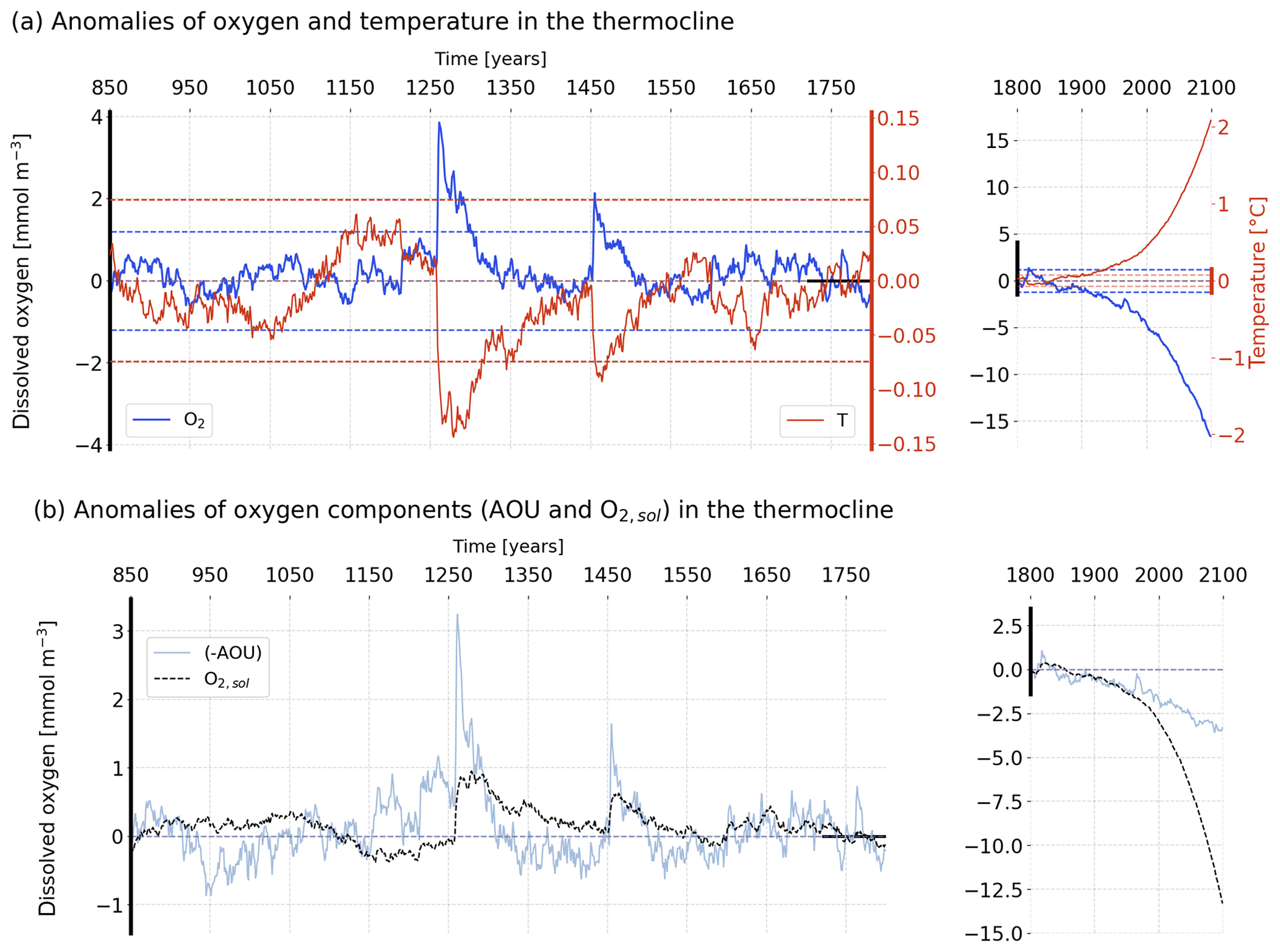
Figure 1Temporal evolution of simulated anomalies in the thermocline (200–600 m) (a) O2 (dark blue) and T (red), and (b) −AOU (light blue) and the O2 solubility component (dashed black) over the last millennium (left) and the historical and future periods (right). The horizontal dashed lines in panel (a) stand for the 2 standard deviation envelopes for O2 (blue) and T (red) computed over the period 850–1800 CE. The anomalies are relative to the pre-industrial reference period (1720–1800 CE).
Last millennium variability in averaged surface ocean T and O2 appears to be dominated by interannual to decadal timescales, whereas large variations on multi-decadal and centennial timescales are simulated for the thermocline and the whole ocean (Fig. 1a, left). During the period 850 to 1800 CE, simulated global mean sea surface temperature (SST) varies generally within an interval of about ±0.3 ∘C and global mean surface O2 within ±1.2 mmol m−3 relative to the reference period (1720–1800 CE). Large global mean SST changes of up to 2 ∘C cooling are modelled after large explosive volcanic eruptions. These are accompanied by large positive anomalies in surface mean O2 of up to 7 mmol m−3. The large post-eruption anomalies decay within a few years to decades in the surface ocean. In the thermocline, annual T varies between −0.15 and +0.1 ∘C, and O2 between −0.7 and 4 mmol m−3 relative to the reference period. These variations occur on multi-decadal to centennial timescales. The imprint of large explosive eruptions is visible as abrupt, sudden perturbations (e.g. in the year 1258), followed by a long-term recovery. Variability for the whole ocean is qualitatively similar to the thermocline, but peak variations are an order of magnitude smaller than for the thermocline depth range.
3.2 ToE, natural variability and anthropogenic change in the thermocline
3.2.1 Time of emergence
Figure 2a and b show the spatial patterns of ToE for O2 and T in the thermocline (200–600 m). These figures show well-defined patterns, with zones of early emergence (before 2020) and zones of late () or no emergence (by 2099) of the anthropogenic signal. In general, the human-induced O2 changes in the thermocline emerge early (before 2020) in high- and midlatitudes, whereas they emerge late or not at all in the tropics (Fig. 2a). Late or no emergence until 2100 is also found in the subtropical Atlantic, western South Pacific and Indian oceans. In contrast, a rather early emergence is simulated in the eastern equatorial Atlantic and Indian Ocean subtropical gyre. These patterns are consistent with the results from Long et al. (2016) and Henson et al. (2017).
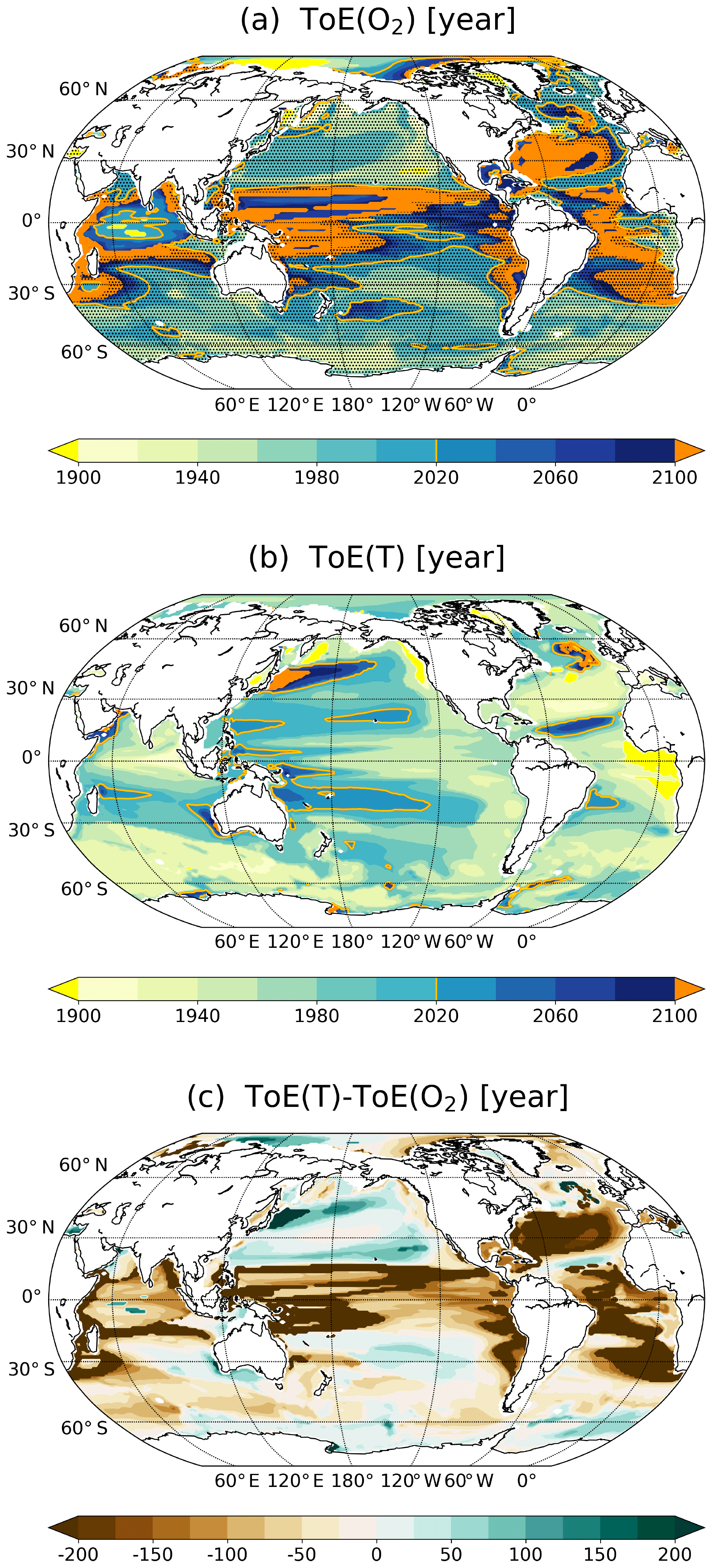
Figure 2ToE of (a) O2, (b) T and (c) their difference in the thermocline (200–600 m). The dashed areas in panel (a) indicate where O2 decreases under RCP8.5. Regions where the anthropogenic signal has not emerged by the end of the 21st century are indicated in orange.
In the case of temperature (Fig. 2b), the anthropogenic signal emerges generally before the end of the 21st century in the thermocline. Exceptions are small areas in the North Atlantic and in the western North Pacific. In contrast to O2, early emergence of the anthropogenic warming is simulated in the subtropical Atlantic gyres and in the equatorial regions. Late emergence is simulated in the subpolar North Atlantic and in the large gyres of the Pacific.
Interestingly, the spatial pattern of the difference between ToE of T minus ToE of O2 resembles the spatial pattern of ToE of O2 (Fig. 2c). The anthropogenic T signal emerges in large regions much earlier than the O2 signal in the thermocline (brown areas; Fig. 2c). These regions include the tropics, the midlatitude Atlantic and the thermocline off the coast of South America. Yet, in some areas, the anthropogenic signal emerges first in O2. The reasons for these results are analysed in Sect. 3.4. The following section is dedicated to a more in-depth analysis of the signal and the noise that both define ToE.
3.2.2 Natural variability and anthropogenic changes
We analyse the magnitude and spatial feature of the noise (Fig. 3a, b) and of the signal (Fig. 3c, d) to understand why a signal emerges early or late. Natural variability of O2 in the thermocline (Fig. 3a) ranges from less than 1 mmol m−3 to more than 10 mmol m−3 (SD±2.50 mmol m−3; 850 to 1800 CE). Variability is small in the core of the O2 minimum zones. In contrast, variability is generally high at the edge of the major oceanic gyres, including transition zones to O2 minimum regions. The anthropogenic signal in O2 remains relatively small in the O2 minimum zones and the subtropical Atlantic gyres (Fig. 3c). O2 is projected to increase in the thermocline in the southern subtropical Indian Ocean gyre region and in the tropical Pacific but to decrease in midlatitudes and high latitudes in the thermocline.
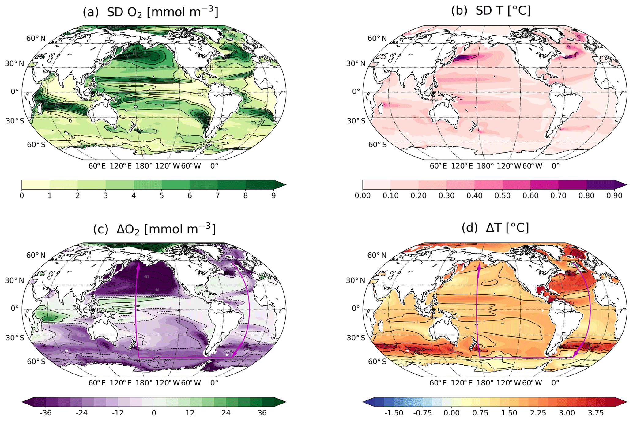
Figure 3Standard deviations for (a) O2 and (b) T as computed for the period 850 to 1800 CE for the thermocline (200–600 m). Anthropogenic changes ((2070–2099) minus (1720–1800)) in (c) O2 and (d) T in the thermocline. O2 and T are annually and vertically averaged and SD and changes are computed from these averaged values. The magenta arrows in panels (c) and (d) indicate the section shown in Fig. 9 (Atlantic: 25∘ W; Southern Ocean: 60∘ S; Pacific: 150∘ W).
By definition, the areas of early emergence (late or no emergence) result from a high (low) signal-to-noise ratio. Locally, a signal may emerge early (late) compared to other regions due to relatively weak (high) variability or a relatively strong (weak) anthropogenic response, or a combination of both. For example, in the region south 30∘ S, simulated O2 concentrations show generally relatively weak natural variability (±2 mmol m−3; Fig. 3a) and large anthropogenic O2 changes ( mmol m−3 by 2100 CE; Fig. 3c) resulting in early ToE. However, in the North Pacific, the early emergence arises from the large anthropogenic signal (−50 mmol m−3 by 2100 CE) despite the intense variability (±10 mmol m−3). In the eastern tropical Atlantic, weak changes and low natural variability result in early emergence. On the contrary, in the western tropical Pacific, the anthropogenic O2 signal has not emerged by 2100 due to the combination of strong natural variability and relatively weak changes.
In general, the temperature signal-to-noise ratio is high in the thermocline, and the emergence of human-induced changes occurs before the end of the 21st century. The thermocline temperature varies naturally by less than ±1 ∘C (Fig. 3b) and the anthropogenic changes are between +1 and +4 ∘C by the end of the 21st century (Fig. 3d). However, the subtropical Pacific gyres, the northern tropical Atlantic and the subtropical Indian gyre show slightly more intense natural variations which delay the emergence of the anthropogenic signal. In parts of the western North Pacific and the North Atlantic, temperature variability in the thermocline is high and the anthropogenic changes remain within the range of natural variability.
3.3 Sensitivity of ToE to methodological differences
Different methodological choices were applied in earlier studies to estimate ToE for precipitation (Giorgi and Bi, 2009), air surface temperature (Karoly and Wu, 2005; Diffenbaugh and Scherer, 2011; Hawkins and Sutton, 2012), SST, pCO2, pH, dissolved inorganic carbon (Keller et al., 2014), primary production or O2 (Rodgers et al., 2015; Carter et al., 2016; Frölicher et al., 2016; Henson et al., 2016, 2017; Long et al., 2016). These different definitions and methods are used to estimate the noise (or natural variability), the anthropogenic signal and the ToE. There seems to be no consensus on the method to estimate ToE. In the following part, in order to gain confidence in the ToE estimates presented above, the impact of different choices on the estimate of ToE is investigated.
3.3.1 Noise estimated from internal variability of a control simulation
The background noise is estimated in many studies from the temporal SD of a control simulation (CTRL) (Hawkins and Sutton, 2012; Maraun, 2013; Long et al., 2016; Henson et al., 2017). In this way, only the internal chaotic variability is taken into account. Accounting for external natural forcing may enlarge the natural O2 variability significantly (Table 1). Indeed, the internal variability represents only 22 % of the total natural variability in the global O2 inventory, 61 % of the variability in the O2 inventory of the thermocline and 47 % of the variability in the global mean surface O2 concentration.
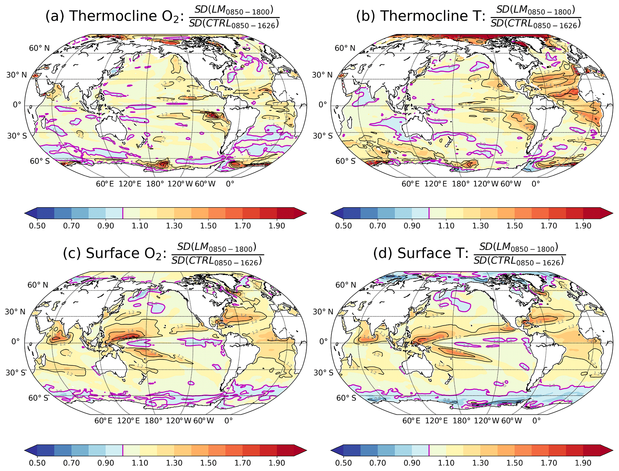
Figure 4Ratio of the SDs from the forced simulation (850–1800 CE) versus those from the control simulation (CTRL) for O2 (left column) and T (right column) for (a, b) the thermocline (200–600 m) and (c, d) the surface. The magenta contours highlight the ratio equal to 1, i.e. where SDs are equal in the forced and control simulation. SDs are computed from annually (all panels) and vertically (panels a–b) averaged values.
Figure 4 compares the externally forced natural variability with the internal variability in each grid cell in the surface layer and in the thermocline (200–600 m) for O2 and T. There are many regions where the ratio between the SD from the forced versus the SD from the CTRL simulation is close to 1, indicating that internal and total natural variability are approximately equal. In particular, forced and internal natural variability in O2 are comparable in most thermocline regions (Fig. 4a). However, there are also regions where natural variability is much larger than internal variability. Indeed, natural variability exceeds internal variability in O2 by more than 50 % in 3 % of the thermocline, while deviations larger than 20 % are found in 18 % of the thermocline. For the temperature, forced variability exceeds internal variability by more than 20 % over a third of the thermocline and by more than 50 % over 10 % of the thermocline. The relative difference between natural and internal variability is thus often smaller for O2 than for T in the thermocline. Turning to the surface ocean, natural variability in O2 and T is substantially larger than internal variability in many low-latitude regions (Fig. 4c, d). Hence, using results from a control simulation to estimate natural variability leads to an underestimation of total natural variability in some specific regions. This affects ToE, as illustrated in Fig. 5. Nevertheless, the results from a control simulation appear to yield a reasonable approximation of simulated natural variability in O2 and T on the local scale in the thermocline. Regions with the largest differences are located at the edges of the subtropical gyres in the North Pacific and the tropical Atlantic (Fig. 5a, b).
Table 1Overview of the standard deviations of T, O2, O2,sol and −AOU, and the corresponding covariance between −AOU and O2,sol for the global mean ocean, the thermocline (200–600 m) and the surface ocean for the control simulation (CTRL) and the forced simulation (850–1800; LM). SD and covariance (COV) are computed from annually and spatially averaged data.

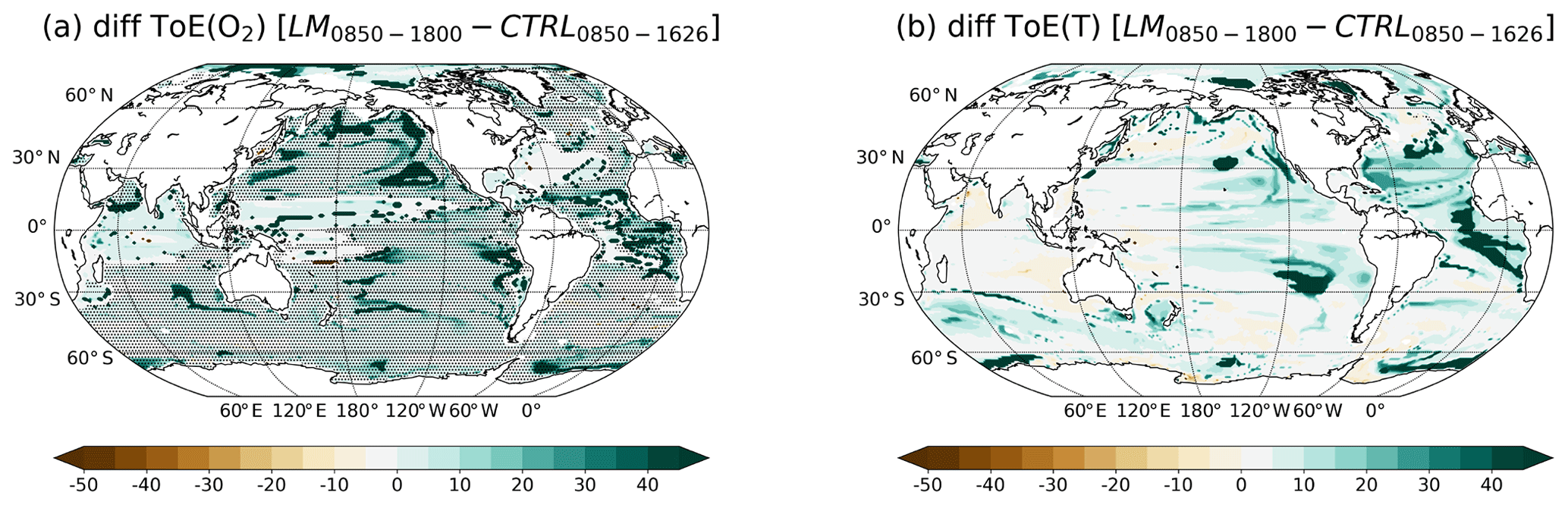
Figure 5Difference of ToE for (a) O2 and (b) T using the SD of the forced simulation (850–1800 CE) minus the ToE using the SD of the control simulation. The dashed areas in panel (a) indicate where O2 decreases under RCP8.5.
3.3.2 Noise estimated over the industrial period
A direct estimation of total natural variability is often not possible because ESM simulations typically start in the 19th century and apply natural plus anthropogenic forcings. Other studies have therefore estimated natural variability from the residual variability (e.g. Keller et al., 2014; Henson et al., 2016) after removing the anthropogenic response from the model output. The residual variability is then defined as the difference between the annual model output and a low-pass-filtered signal. Here, a spline with a cut-off period of 40 years is used to compute the filtered signal. Then, the standard deviation of the residual variability is computed for the period 1850 to 2005 CE. Surprisingly, the SD of O2 and T in the thermocline as computed from the residual variability is much smaller than that computed from the last millennium (LM) simulation in many regions (Fig. 6a, b). Particularly large differences (100 % of LM SD or more) are found in the Atlantic and high-latitude regions for T and O2 and in large parts of the Pacific for O2. The stronger variability in LM compared to the residual variability likely results from low-frequency variability included in LM but removed by the spline in the residuals. As a consequence, O2 and T in the thermocline emerge earlier when using SD from the residuals instead of SD from the 850 to 1800 CE period to compute ToE (Fig. 6c, d).

Figure 6Ratio of the SDs of the forced simulation computed over the period 850–1800 CE and of the residual variability computed over the period 1850–2005 CE using a cut-off period of 40 years for (a) O2 and (b) T. Difference of ToE using the SD of the forced simulation minus the ToE using the residual variability for (c) O2 and (d) T. The magenta contours highlight the ratio equal to 1, i.e. where SDs are equal. SDs are computed from annually and vertically averaged values between 200 and 600 m.
Estimates of noise may further be sensitive to the choice of the period. Because fully coupled millennial-scale simulations are expensive and relatively rare, we compare the SD of T and O2 in the thermocline in the forced LM simulation for the period 850–1800 CE versus the shorter pre-industrial reference period 1720–1800 CE (Fig. A6a, b). In a large part of the thermocline, SD in T and O2 are similar (within ±10 %), reflecting a similar estimated natural variability. Differences in SD are, for example, found in regions of the South Pacific, the eastern North Pacific, the Arctic Ocean and for O2 in the Arabian Sea. For O2, substantially earlier ToE values are estimated in large parts of the Pacific, the Arctic and the Southern Ocean when using the pre-industrial period to approximate the natural variability (Fig. A6a). However, changes in oxygen are estimated to appear later in some parts of the equatorial Atlantic, in the Arabian Sea and in a few grid cells in the Pacific and Arctic. Similarly, earlier ToE values for T are found, for example, in large parts of the Pacific when using the variability from the pre-industrial period (Fig. A6b). The results suggest that a century-long period of the forced simulation may not yield robust results for variability and ToE in all regions.
3.4 Apparent oxygen utilisation, O2 solubility, ventilation and organic matter cycling
We analyse AOU and the O2 solubility component (O2,sol) in order to gain insight into the processes underlying O2 variations. O2,sol variations are driven by SST changes and AOU variations mainly reflect the imprint of changes in water mass ventilation and in the remineralisation of organic matter. Here, ventilation is diagnosed by an ideal age tracer, and changes in remineralisation of organic matter are linked to the production of organic matter.
3.4.1 Natural variability
Changes in AOU largely explain most of the pre-industrial variations in O2 with a generally small role for O2,sol both at the global scale and on average in the thermocline (Figs. 1a, b and A5a). The O2,sol component contributes nonetheless notably to the O2 changes after the large volcanic eruptions in 1258 and 1452. This general dominance of AOU over O2,sol during PI contrasts with the industrial period, during which changes in O2,sol contribute for half of the global ocean O2 decrease (Fig. A5a). An even larger relative contribution of O2,sol is simulated for the spatially averaged thermocline signal (Fig. 1b). Changes in AOU in the thermocline remain small over the industrial period due to the compensation of regionally opposed responses, as described below. The O2 variations at the surface are, unsurprisingly, primarily caused by changes in solubility (O2,sol; Fig. A5b).
Quantification of the natural variability of O2 can be split into the contributions from individual components given in Eq. (1) following:
Var() stands for the variance of the variable and equals the square of SD. Both metrics are positive by definition. The sign of the covariance between O2,sol and indicates whether the contributions from O2,sol and −AOU enhance or partly cancel each other. If is negative, for example, the resulting Var(O2) will be smaller than the sum of Var(O2,sol) and Var(−AOU) and the two components partly cancel each other. On the contrary, they have an additive effect when their covariance is positive.
Table 1 gathers the SD of O2 and its components and the corresponding covariance in the global averaged surface ocean, thermocline and world ocean for the control simulation and the forced simulation (850–1800 CE). is negative in CTRL in all three water bodies. Hence, O2,sol and −AOU partly compensate for each other in CTRL. is also negative in LM for the surface ocean. This implies that changes in solubility are partly compensated by changes in air–sea O2 disequilibrium. In contrast, is positive in the LM simulation for the global ocean and the spatially averaged thermocline during the pre-industrial period. Hence, changes in O2,sol and −AOU are positively correlated and reinforce each other on average. In conclusion, the natural forcing leads to a positive correlation of −AOU and O2,sol. This statistical analysis is consistent with the discussion on O2 perturbations above: −AOU and O2,sol change hand in hand after large volcanic eruptions in the global mean and in the global thermocline (Fig. 1a, b). The variability in CTRL is not only smaller than in LM but apparently also different in terms of underlying physical and biogeochemical mechanisms and in their interactions.
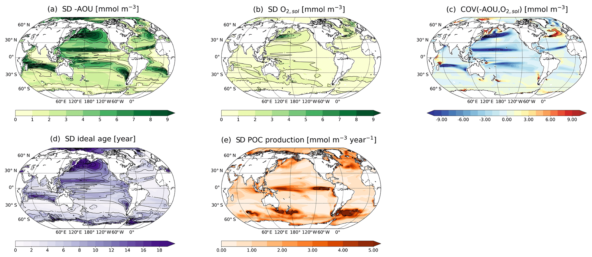
Figure 7Standard deviation of annually and vertically averaged (200–600 m) (a) −AOU, (b) O2,sol, (d) ideal age and (e) particulate organic carbon (POC) production during the last millennium (850–1800 CE) and (c) the corresponding covariance between −AOU and O2,sol.
The spatial pattern of the natural variability in O2 (Fig. 3a) can largely be attributed to −AOU (Fig. 7a). O2,sol variations have generally a limited impact on O2 in the thermocline (Fig. 7b). By definition, O2,sol is largely congruent with the previously discussed pattern of SD(T) (Fig. 3b). Nevertheless, in the high-variability regions in the western North Pacific and the northern North Atlantic, SD(O2,sol) is of the same order of magnitude as SD(−AOU). The latter resembles the pattern of SD for ideal age (Fig. 7d). This suggests that a significant fraction of the variability in −AOU (and thus O2) is driven by changes in circulation and water mass age. Variability in POC production in the surface layer (Fig. 7e), indicative of water column remineralisation of organic material, may also contribute to the variability in −AOU in the thermocline. For example, in the northern North Atlantic, SD in POC production and −AOU is relatively large, while SD in ideal age is low. On the other hand, the large SDs in POC production in parts of the Southern Ocean are not reflected in SD(−AOU). is strongly negative in some regions with large variability in −AOU (Fig. 7c). These regions, as discussed in Sect. 3.2, are located at the boundaries of major gyres. This suggests that changes in −AOU and O2,sol partly compensate for each other in these regions. An exception is the boundary region between the subtropical and subpolar gyres in the North Atlantic, where the two components tend to enhance each other and therefore increase O2 variability.
3.4.2 Anthropogenic change
Next, we address the pattern of anthropogenic changes in O2,sol (ΔO2,sol) and in −AOU (Δ(−AOU)) in the thermocline (Figs. 8 and 9). ΔO2,sol shows a spatially coherent decrease as dictated by the global warming pattern (Fig. 3d). In contrast, Δ(−AOU) shows a strong spatial pattern in the thermocline with positive values in the tropics, the Arctic and subtropical Atlantic and negative values in the midlatitude and high-latitude Pacific as well as the Southern Ocean and the subtropical Indian and the Pacific Ocean. Regional changes in −AOU largely balance each other, explaining the small change in spatially averaged −AOU (Fig. 1b). The anthropogenic increase in O2 (Fig. 3c) in parts of the tropical thermocline is attributed to the increase in −AOU, partly offset by the decrease in O2,sol, while the anthropogenic O2 decrease in the northern Pacific and the Southern Ocean results from a decrease in both −AOU and O2,sol.
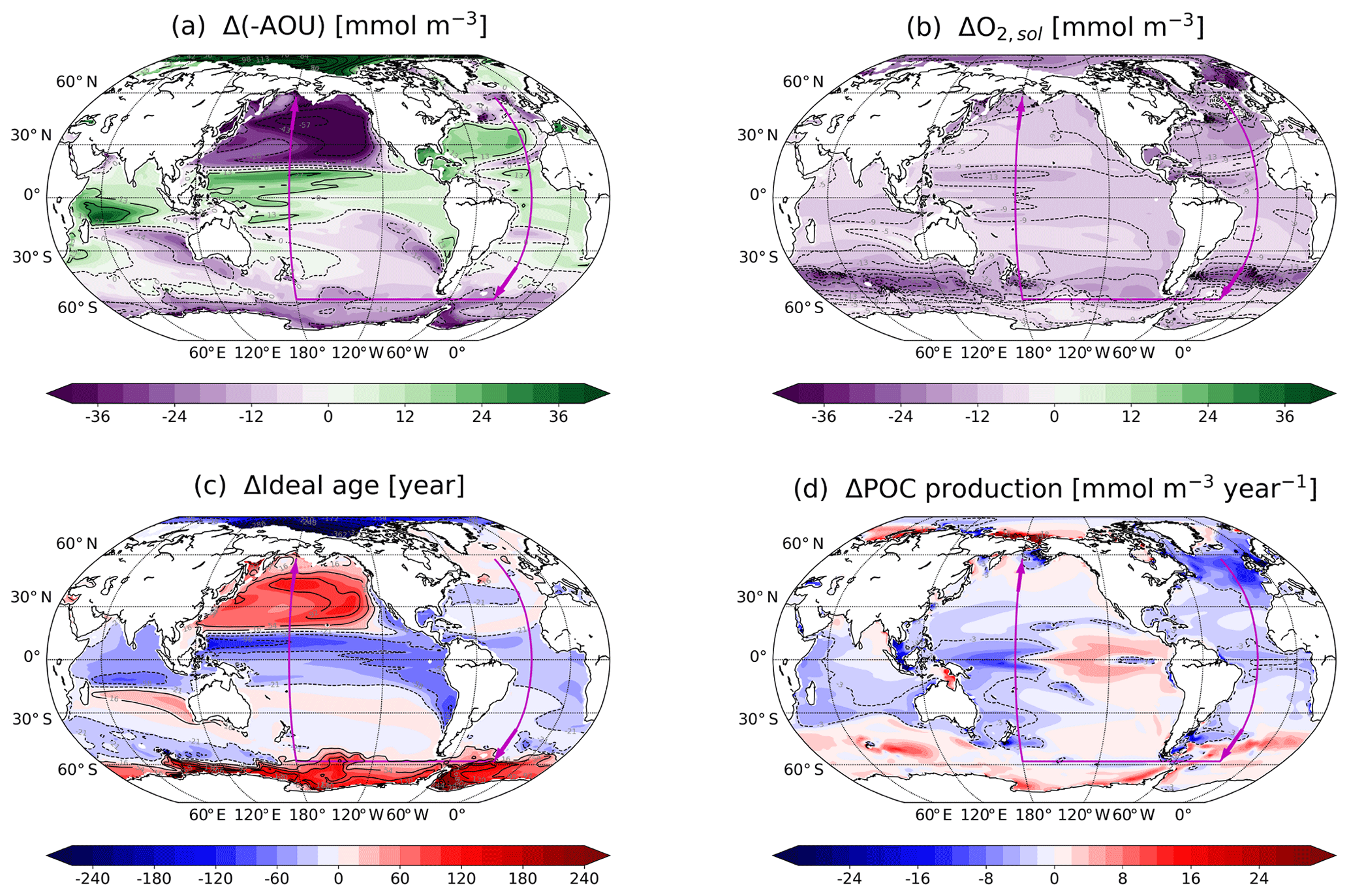
Figure 8Anthropogenic changes ((2070–2099 CE) minus (1720–1800 CE)) in (a) −AOU, (b) O2,sol, (c) ideal age and (d) POC production. The results are averaged between 200 and 600 m, except for POC production, which is averaged between the surface and 200 m. The magenta arrows indicate the section path used in Fig. 9 (Atlantic: 25∘ W; Southern Ocean: 60∘ S; Pacific: 150∘ W).
Δ(−AOU) in the thermocline is mainly driven by changes in ventilation and modulated by changes in remineralisation rates (Fig. 8c, d). The increase in ideal age and the increase in POC production (indicative of an increase in remineralisation rate) explain the decrease in −AOU in the Southern Ocean. By contrast, in the western tropical Pacific, the equatorial Indian and the Atlantic oceans, the combination of a decrease in water mass age and in POC production explains the increase in −AOU over the industrial period and the 21st century. In the eastern tropical Pacific and in the North Pacific, the impacts of changes in ventilation are partly mitigated by changes in organic matter remineralisation rate.
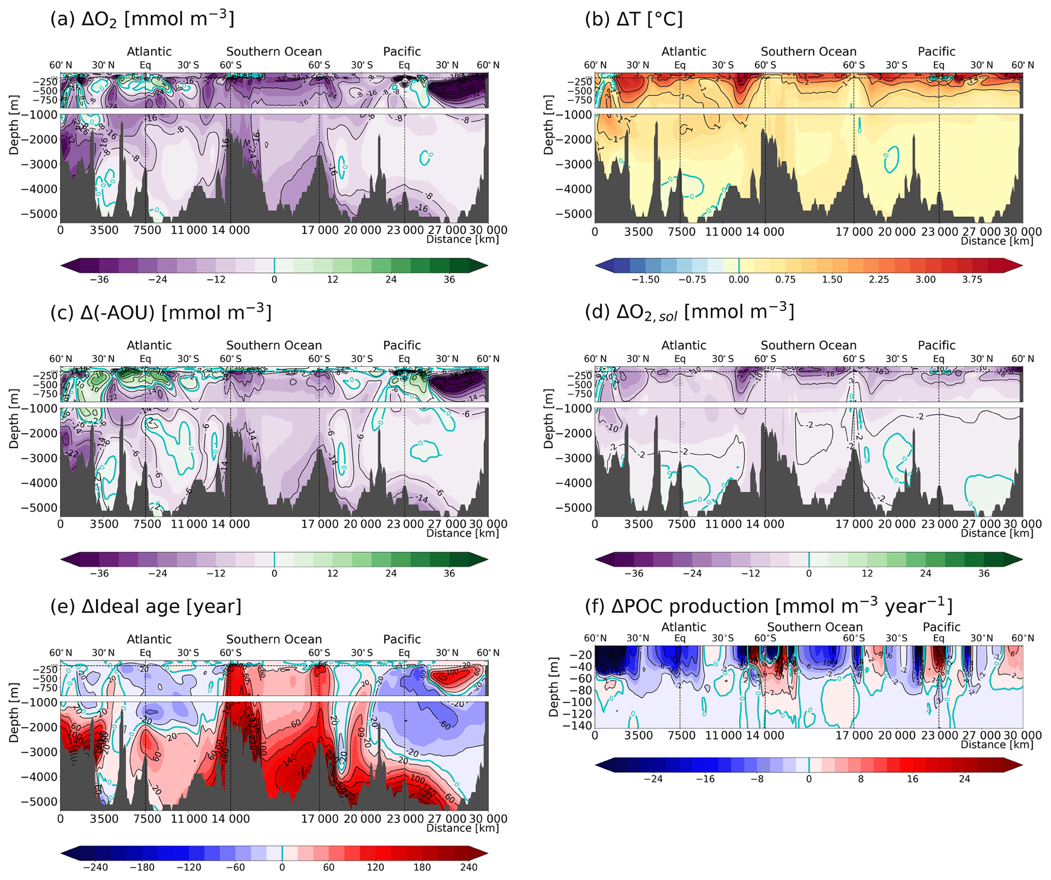
Below the thermocline and in the deep ocean, O2 decreases over the industrial period and the 21st century as both −AOU and O2,sol decrease (Fig. 9). The decrease in −AOU is again mainly explained by an increase in ideal age. Changes in ideal age in the deep Atlantic, Southern Ocean and Pacific partly exceed 150 years and indicate a general reduction in the deep water mass formation over the industrial period and the 21st century in the simulation.
3.5 ToE of O2 components
Both the variability and the anthropogenic signal of O2 in the thermocline are driven primarily by changes in −AOU, the former of which is influenced in part by changes in O2,sol. The question arises whether the signal of −AOU or of O2,sol emerge earlier than the signal of O2. As O2,sol is a function of T, ToE(O2,sol) is very similar to ToE(T) and we refer to the previous discussion on ToE(T) (Fig. 2b) and its difference to ToE(O2) (Fig. 2c). Interestingly, the −AOU and O2 signals seem to emerge around the same time in the thermocline in the Pacific and Indian subtropical gyres (Fig. 10b). But the signal of −AOU emerges later in the thermocline in many regions including the subtropical oceans in the Southern Hemisphere, while it emerges earlier in the tropics and in the subtropical gyres of the Atlantic as well as south of Madagascar. This suggests that anthropogenic changes in −AOU might be detectable earlier in large oceanic regions. However, the specific results may be model-dependent and need to be confirmed by other models or by observations. Earlier emergence of −AOU than O2 is generally found in regions with a positive change in −AOU and thus in regions where −AOU and O2,sol partly offset each other. Late emergence in −AOU is found in regions with a small anthropogenic change in −AOU.
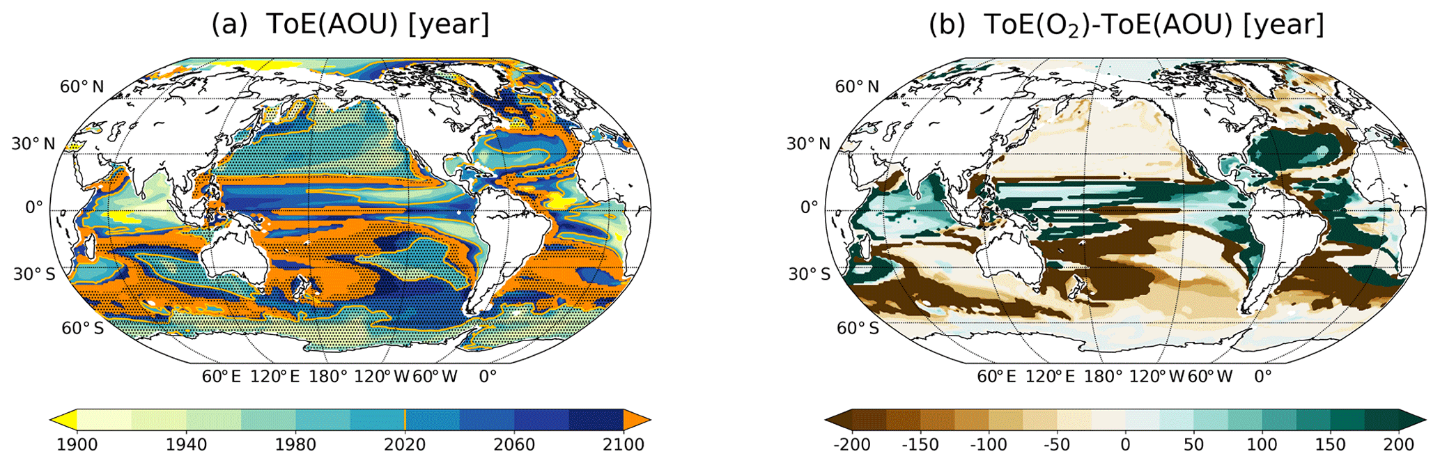
Figure 10ToE of (a) −AOU, (b) O2,sol in the thermocline (200–600 m). The dashed areas in panel (a) indicate where −AOU decreases under RCP8.5. Regions where the anthropogenic signal has not emerged by the end of the 21st century are indicated in orange for AOU. (b) Difference of the ToE for O2 and the ToE of −AOU in the thermocline (200–600 m).
We have analysed the natural variability over the last millennium and anthropogenic trends of marine oxygen (O2) and temperature (T) in simulations using the Community Earth System Model (CESM). The relative roles of the internal and forced natural variability were quantified. We have also determined the time of emergence (ToE) of T, O2 and apparent oxygen utilisation (AOU) in the thermocline.
We find that anthropogenic deoxygenation and warming in the thermocline has today already left the bounds of natural variability on the global scale. By 2020, these signals have emerged in over 60 % and 90 % of the thermocline area, respectively (Fig. 11). By the end of this century, these values are approaching 100 % if greenhouse gas emissions continue unabated. This presents an increasing risk for the function and services of marine ecosystems (Pörtner et al., 2014). ToE for O2 is relatively early in the midlatitude and high-latitude thermocline and late in the tropical ocean and subtropical Atlantic, in agreement with earlier work (Long et al., 2016; Henson et al., 2017). Temperature ToE has not been analysed in the thermocline in earlier studies. In CESM, ToE is relatively early for T in the thermocline of eastern boundary systems, the subtropical Atlantic and in large parts of the Southern Ocean but late in many subtropical regions and in large parts of the North Pacific.
A large O2 decline is simulated by CESM for the future in the North Pacific thermocline, in agreement with other models (Bopp et al., 2013; Cocco et al., 2013). This region is characterised by particularly large changes in ventilation. As an interesting consequence, the anthropogenic O2 signal is detectable earlier than the anthropogenic temperature signal in large parts of the northern North Pacific. Along the same line, Keller et al. (2015) show that a potential weakening of the El Niño–Southern Oscillation (ENSO) variability is verifiable earlier and more widespread for carbon cycle tracers than for temperature, and Séférian et al. (2014) highlight the multi-year predictability of tropical productivity. This corroborates earlier suggestions by Joos et al. (2003) that measurements of O2, or, more generally, multi-tracer observations, are critical in detecting or predicting anthropogenic changes.
For a better understanding of these results, we have analysed the natural variability and the anthropogenic response of the respiration (−AOU) and solubility (O2,sol) components of O2. Variations in AOU dominate variations in O2 during the last millennium, as well as the local response to anthropogenic emissions in the thermocline. For the globally averaged thermocline, internal variability in AOU and in O2,sol are negatively correlated and partly offset each other. In contrast, the total natural variability of these two components is positively correlated and thus enforces variability in O2 in the global thermocline (Table 1). Under human activities, changes in AOU and O2,sol partly cancel each other in the tropical thermocline and in the subtropical Atlantic Ocean, in accordance with Bopp et al. (2017). Moreover, AOU (thus O2) variability and its signal are explained by changes in water mass ventilation, with a smaller role for changes in biological productivity (Figs. 8 and 9). Strongly reduced ventilation in the northern North Pacific therefore drives the early O2 emergence. This suggests that weakened ventilation precedes warming in the thermocline in this region.
The comparison between the transient last millennium simulation and the corresponding control simulation shows that both the naturally forced and the internal variability contributed to the simulated climate and biogeochemical variations of the last millennium. The internal variability arises from the inherent and partly chaotic variability of the climate system (Frölicher et al., 2009; Deser et al., 2012; Resplandy et al., 2015). The natural forced climate variability arises from explosive volcanism and from changes in solar irradiance on interannual to centennial timescales (Wanner et al., 2008). The relative importance of forced variability is particularly large when considering large-scale averages (Table 1, Fig. 4) but can also be substantial on the local scale. Our results imply that natural forced variations should not be neglected when comparing century-scale anthropogenic climate change to natural climate variability.
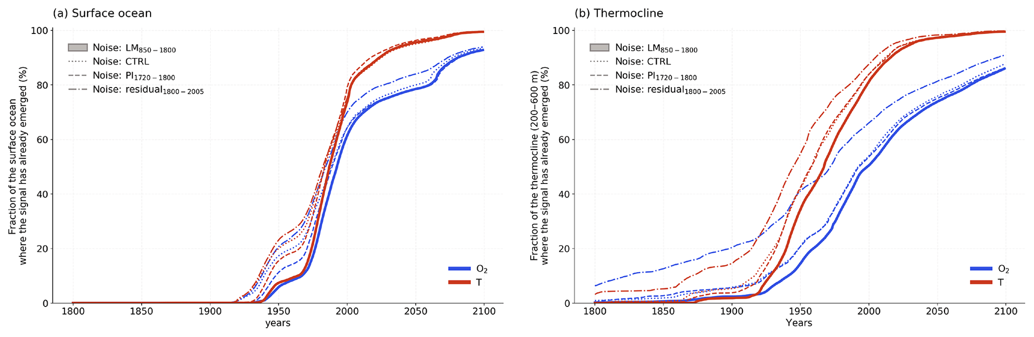
Figure 11Fraction of the (a) surface ocean and (b) thermocline (200–600 m) where the signal has already emerged in oxygen (blue) and temperature (red) for different definitions of the background noise: (i) naturally forced variability during the last millennium (850–1800 CE, LM; solid), (ii) internal variability (CTRL; dotted), (iii) naturally forced variability during the pre-industrial period (1720–1800 CE, PI; dashed), (iv) residual variability using a low-pass filter (cut-off period of 40 years, residual; dashed dotted).
Moreover, we show that ToE is highly sensitive to the method applied for estimating the natural variability. We have estimated variability from a forced simulation over the last millennium (850–1800 CE), over the period 1720 to 1800 CE, and from a control simulation. As expected, using variability from the control and the short period yields, in general, an earlier emergence of the anthropogenic signal than when using variability from the last millennium simulation (Fig. 11). These two estimates of noise do not capture the full natural variability of the last millennium. Yet, differences in estimated ToE and noise are often modest on the local scale (Figs. 2, 4 and 11). In addition, we have tested the use of the “residual” variability of a time series to estimate noise. The long-term trend in the industrial period (1850–2005 CE) data is removed by a low-pass filter; the standard deviation of the remaining annual anomalies provides then an estimate of the noise. This yields a much smaller variability than estimated from the last millennium output and thus a much earlier ToE (Figs. 6 and 11). Applying a smoothing-spline cut-off period of 80 or 100 years instead of 40 years leaves a higher variability but the full last millennium variability is still underestimated (not shown). In conclusion, it might be appropriate, though not ideal, to use the results from a control simulation to estimate natural variability, as last millennium Earth system simulations extended towards the future period are still rare.
Alternatively, large ensemble simulations for the industrial period and the future will become available within CMIP6. Different ensembles including or excluding anthropogenic forcing (Stott et al., 2000) and including or excluding natural forcing may be used to disentangle the individual contributions to trends and variability. Some model centres may also wish to generate large ensemble simulations for the last millennium to study natural variability over the more recent pre-industrial period (Jungclaus et al., 2010).
However, there are still some uncertainties in our results, and some are linked to the relatively coarse resolution of the CESM model of the order of 1∘. Larger variability may be found on smaller scales. For example, Long et al. (2016) document that interannual variability from the Hawaii Ocean Time-Series (HOT) station is about a factor of 2 larger than the variability at the same location in CESM. Another source of error is structural model uncertainty. Comparison with observations (Sect. 2.1.3) and multi-model studies shows weaknesses of the current class of Earth system models in simulating the observed O2 distribution and variability. Projections of anthropogenic O2 change are particularly uncertain in low-oxygenated waters (Bopp et al., 2013; Cocco et al., 2013).
O2 changes will likely continue beyond 2100 CE. We find a strong link between changes in O2, AOU and ideal age, with a shift to older water mass ages accompanied by a shift to lower O2. By 2100, ideal age in the near-bottom waters of the Southern Ocean and the deep Pacific has increased by up to 240 years and O2 decreased by around 16 to 20 mmol m−3 relative to pre-industrial period. These anomalies are likely to spread further into the deep ocean. A long-term reduction in deep ocean ventilation and O2 under anthropogenic forcing is consistent with results from Earth system models of intermediate complexity (Schmittner et al., 2008; Battaglia and Joos, 2018). For example, Battaglia and Joos (2018) find a large, transient decline in deep ocean O2 and in the global O2 inventory by as much as 40 % in scenarios where radiative forcing is stabilised in 2300 CE. In their simulations, deoxygenation peaks about a thousand years after the forcing stabilisation and new steady-state conditions are established only after 8000 CE. The CESM results also support the notion of long-term deep ocean deoxygenation.
In conclusion, we find that natural radiative forcing arising from explosive volcanism and solar irradiance changes contributes notably to the overall past variability of marine O2 and temperature. We simulate large and widespread ocean deoxygenation under anthropogenic forcing and suggest that large parts of the thermocline are already experiencing environmental conditions that are outside the range of natural variability of the last millennium.
Data are available on request.
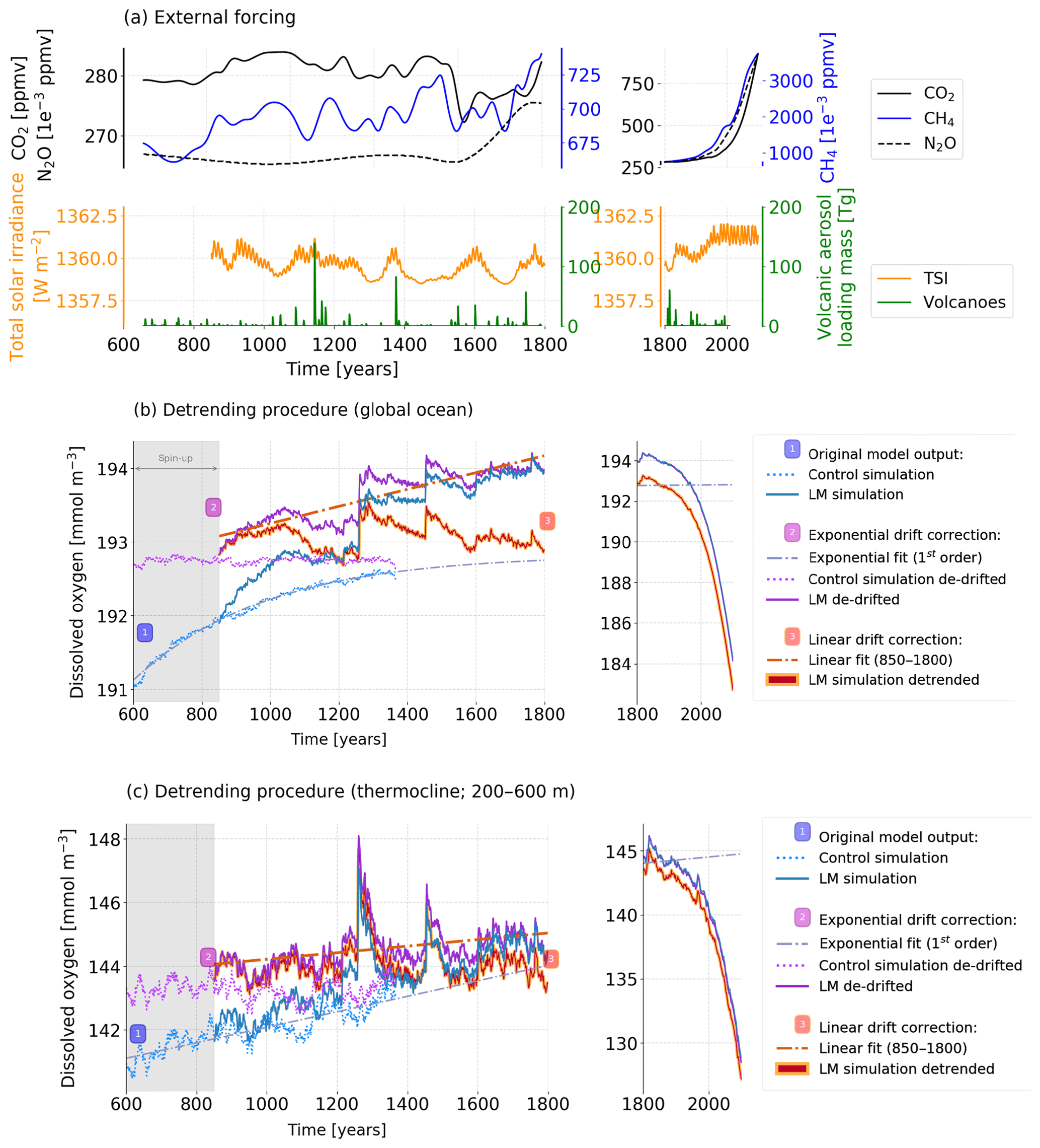
Figure A1(a) Time series of the main external forcings applied to the forced simulation: total solar irradiance (W m−2) at the top of the atmosphere in orange, stratospheric volcanic aerosol load (Tg) in green and the greenhouse gases CO2 (solid black line), N2O (dashed black line) and CH4 (solid blue line) (ppmv). Illustration of the two-step procedure to remove model drift and millennial-scale trends at each grid point shown in (b) the global mean ocean and (c) the thermocline (200–600 m). The original, annually averaged outputs from the control (CTRL) and the forced simulations are shown by dashed and solid blue lines, respectively (1). The results of the CTRL are fitted by an exponential function with one timescale and extrapolated towards equilibrium (dashed line). The exponential curve is subtracted from and the equilibrium value added to the original outputs to obtain the purple curves (2) (dotted: CTRL, solid: forced simulation). The remaining multi-millennial trend in the forced simulation is removed using a linear fit (850–1800 CE), leading to the red curve (3).
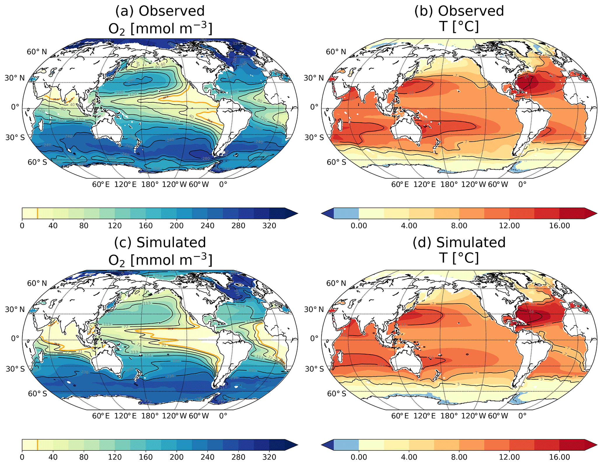
Figure A2Observation-based (a, b) versus simulated (c, d; 1986–2005) oxygen concentration (a, c) and temperature (b, d) in the thermocline (200–600 m). Data are from (a) Garcia et al. (2014) and (b) Locarnini et al. (2013).
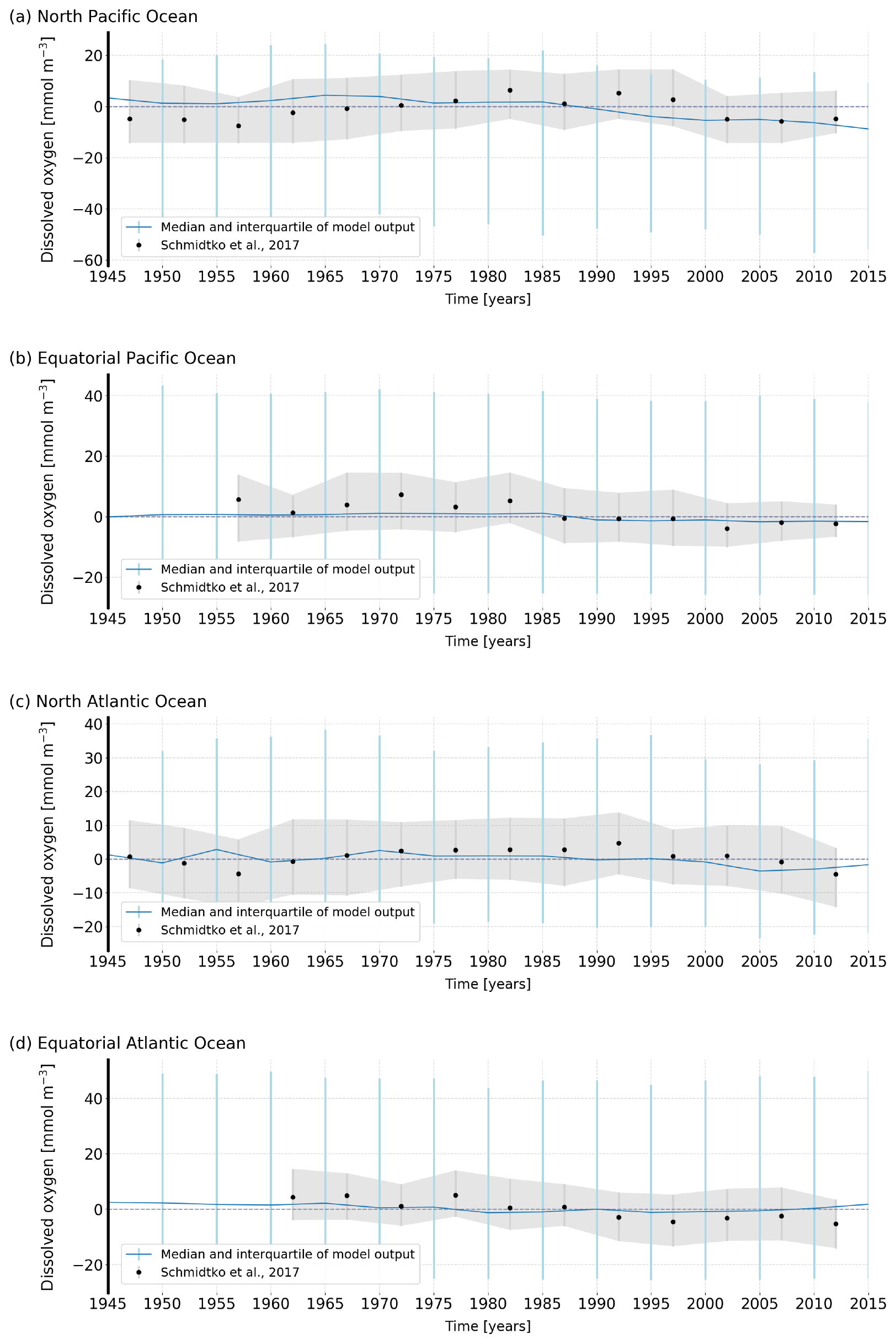
Figure A3Comparison of the semi-decadal median and interquartile range of the simulated O2 concentration (blue) and the historical data from Schmidtko et al. (2017) (grey) over the (a) North Pacific, (b) equatorial Pacific, (c) North Atlantic and (d) equatorial Atlantic.

Figure A4Illustration of the ToE method. The example is for the thermocline (200–600 m) and grid cells located at 158∘ W and 22∘ N near Hawaii. The SD of the detrended, annually and vertically (200–600 m) averaged data (blue) for the period 850–1800 CE is used to define the “noise” or bounds of natural variability which is set to ±2 SD (blue area). The annually and vertically averaged data are fitted with a spline using a cut-off period of 40 years (light blue). ToE is the point in time when the spline crosses and leaves the bounds of natural variability; here, ToE is 1984 and indicated by the vertical dashed line. All data are anomalies relative to the pre-industrial period (1720–1800 CE; yellow).
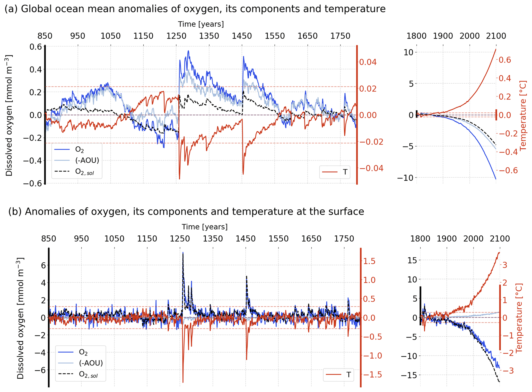
Figure A5Temporal evolution of simulated anomalies in (a) global mean O2 (dark blue), −AOU (light blue), the O2 solubility component (dashed black) and T (red) over the last millennium (left) and the historical and future periods (right). The horizontal dashed lines stand for the 2 standard deviation envelopes for O2 (blue) and T (red) computed over the period 850–1800 CE. (b) Same as (a) but for the surface. The anomalies are relative to the pre-industrial reference period (1720–1800 CE).
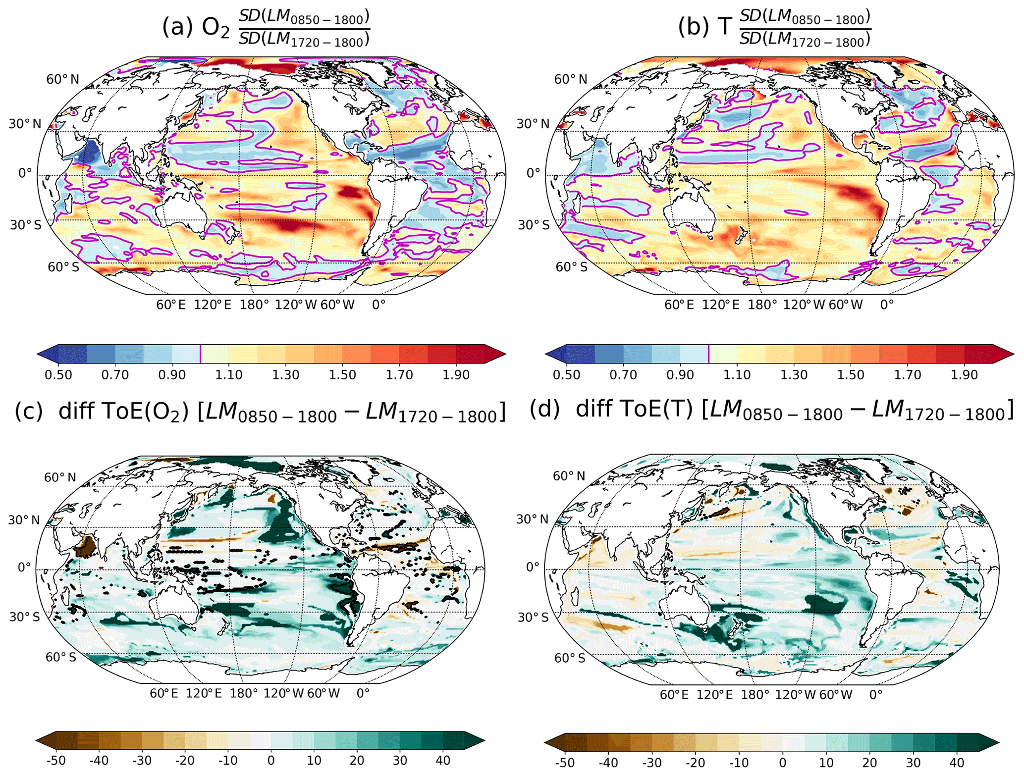
Figure A6Ratio of the SDs of the forced simulation computed over the period 850–1800 CE and over the period 1720–1800 CE for (a) O2 and (b) T. Difference of ToE using the SD of the forced simulation over the period 850–1800 CE minus the ToE using the SD of the same simulation but over the pre-industrial period (1720–1800 CE) for (c) O2 and (d) T. The magenta contours highlight the ratio equal to 1, i.e. where SDs are equal. SDs are computed from annually and vertically averaged values between 200 and 600 m.
The authors declare that they have no conflict of interest.
This article is part of the special issue “The 10th International Carbon Dioxide Conference (ICDC10) and the 19th WMO/IAEA Meeting on Carbon Dioxide, other Greenhouse Gases and Related Measurement Techniques (GGMT-2017) (AMT/ACP/BG/CP/ESD inter-journal SI)”. It is a result of the 10th International Carbon Dioxide Conference, Interlaken, Switzerland, 21–25 August 2017.
This study is funded by the Oeschger Centre for Climate Change Research and the Swiss National Science Foundation (no. 200020_172476). We thank Christoph Raible and Flavio Lehner for providing CESM output and Thomas Frölicher and Oliver Aumont for discussion. Fortunat Joos and Angélique Hameau thank the Swiss National Supercomputing Centre (CSCS) for computing support.
This paper was edited by Christoph Heinze and reviewed by two anonymous referees.
Ammann, C. M., Joos, F., Schimel, D. S., Otto-Bliesner, B. L., and Tomas, R. A.: Solar Influence on Climate during the Past Millennium: Results from Transient Simulations with the NCAR Climate System Model, P. Natl. Acad. Sci. USA, 104, 3713–3718, https://doi.org/10.1073/pnas.0605064103, 2007. a
Andres, R. J., Boden, T. A., Bréon, F.-M., Ciais, P., Davis, S., Erickson, D., Gregg, J. S., Jacobson, A., Marland, G., Miller, J., Oda, T., Olivier, J. G. J., Raupach, M. R., Rayner, P., and Treanton, K.: A synthesis of carbon dioxide emissions from fossil-fuel combustion, Biogeosciences, 9, 1845–1871, https://doi.org/10.5194/bg-9-1845-2012, 2012. a
Armstrong, R. A., Lee, C., Hedges, J. I., Honjo, S., and Wakeham, S. G.: A New, Mechanistic Model for Organic Carbon Fluxes in the Ocean Based on the Quantitative Association of POC with Ballast Minerals, Deep-Sea Res. Pt. II, 49, 219–236, https://doi.org/10.1016/S0967-0645(01)00101-1, 2001. a
Bakun, A.: Climate Change and Ocean Deoxygenation within Intensified Surface-Driven Upwelling Circulations, Philos. T. R. Soc. A, 375, 20160327, https://doi.org/10.1098/rsta.2016.0327, 2017. a
Bard, E., Raisbeck, G., Yiou, F., and Jouzel, J.: Solar Irradiance during the Last 1200 Years Based on Cosmogenic Nuclides, Tellus B, 52, 985–992, https://doi.org/10.3402/tellusb.v52i3.17080, 2000. a
Battaglia, G. and Joos, F.: Hazards of decreasing marine oxygen: the near-term and millennial-scale benefits of meeting the Paris climate targets, Earth Syst. Dynam., 9, 797–816, https://doi.org/10.5194/esd-9-797-2018, 2018. a, b, c
Bopp, L., Resplandy, L., Orr, J. C., Doney, S. C., Dunne, J. P., Gehlen, M., Halloran, P., Heinze, C., Ilyina, T., Séférian, R., Tjiputra, J., and Vichi, M.: Multiple stressors of ocean ecosystems in the 21st century: projections with CMIP5 models, Biogeosciences, 10, 6225–6245, https://doi.org/10.5194/bg-10-6225-2013, 2013. a, b, c, d
Bopp, L., Resplandy, L., Untersee, A., Mezo, P. L., and Kageyama, M.: Ocean (de)Oxygenation from the Last Glacial Maximum to the Twenty-First Century: Insights from Earth System Models, Philos. T. R. Soc. A, 375, 20160323, https://doi.org/10.1098/rsta.2016.0323, 2017. a, b, c
Brandt, P., Bange, H. W., Banyte, D., Dengler, M., Didwischus, S.-H., Fischer, T., Greatbatch, R. J., Hahn, J., Kanzow, T., Karstensen, J., Körtzinger, A., Krahmann, G., Schmidtko, S., Stramma, L., Tanhua, T., and Visbeck, M.: On the role of circulation and mixing in the ventilation of oxygen minimum zones with a focus on the eastern tropical North Atlantic, Biogeosciences, 12, 489–512, https://doi.org/10.5194/bg-12-489-2015, 2015. a
Breitburg, D., Levin, L. A., Oschlies, A., Grégoire, M., Chavez, F. P., Conley, D. J., Garçon, V., Gilbert, D., Gutiérrez, D., Isensee, K., Jacinto, G. S., Limburg, K. E., Montes, I., Naqvi, S. W. A., Pitcher, G. C., Rabalais, N. N., Roman, M. R., Rose, K. A., Seibel, B. A., Telszewski, M., Yasuhara, M., and Zhang, J.: Declining Oxygen in the Global Ocean and Coastal Waters, Science, 359, eaam7240, https://doi.org/10.1126/science.aam7240, 2018. a
Brovkin, V., Lorenz, S. J., Jungclaus, J., Raddatz, T., Timmreck, C., Reick, C. H., Segschneider, J., and Six, K.: Sensitivity of a Coupled Climate-Carbon Cycle Model to Large Volcanic Eruptions during the Last Millennium, Tellus B, 62, 674–681, https://doi.org/10.1111/j.1600-0889.2010.00471.x, 2010. a
Cabré, A., Marinov, I., Bernardello, R., and Bianchi, D.: Oxygen minimum zones in the tropical Pacific across CMIP5 models: mean state differences and climate change trends, Biogeosciences, 12, 5429–5454, https://doi.org/10.5194/bg-12-5429-2015, 2015. a
Camenisch, C., Keller, K. M., Salvisberg, M., Amann, B., Bauch, M., Blumer, S., Brázdil, R., Brönnimann, S., Büntgen, U., Campbell, B. M. S., Fernández-Donado, L., Fleitmann, D., Glaser, R., González-Rouco, F., Grosjean, M., Hoffmann, R. C., Huhtamaa, H., Joos, F., Kiss, A., Kotyza, O., Lehner, F., Luterbacher, J., Maughan, N., Neukom, R., Novy, T., Pribyl, K., Raible, C. C., Riemann, D., Schuh, M., Slavin, P., Werner, J. P., and Wetter, O.: The 1430s: a cold period of extraordinary internal climate variability during the early Spörer Minimum with social and economic impacts in north-western and central Europe, Clim. Past, 12, 2107–2126, https://doi.org/10.5194/cp-12-2107-2016, 2016. a, b
Carter, B. R., Frölicher, T. L., Dunne, J. P., Rodgers, K. B., Slater, R. D., and Sarmiento, J. L.: When Can Ocean Acidification Impacts Be Detected from Decadal Alkalinity Measurements?, Global Biogeochem. Cy., 30, 2015GB005308, https://doi.org/10.1002/2015GB005308, 2016. a, b, c
Chikamoto, M. O., Timmermann, A., Yoshimori, M., Lehner, F., Laurian, A., Abe-Ouchi, A., Mouchet, A., Joos, F., Raible, C. C., and Cobb, K. M.: Intensification of Tropical Pacific Biological Productivity Due to Volcanic Eruptions, Geophys. Res. Lett., 43, 2015GL067359, https://doi.org/10.1002/2015GL067359, 2016a. a
Chikamoto, M. O., Timmermann, A., Yoshimori, M., Lehner, F., Laurian, A., Abe-Ouchi, A., Mouchet, A., Joos, F., Raible, C. C., and Cobb, K. M.: Volcanic Eruptions Boost Tropical Pacific Biological Productivity, Geophys. Res. Lett., 43, 1184–1192, https://doi.org/10.1002/2015GL067359, 2016b. a
Christensen, J., Hewitson, B., Busuioc, A., Chen, A., Gao, X., Held, I., Jones, R., Kolli, R. K., Kwon, W.-T., Laprise, R., Magaña Rueda, V., Mearns, L., Menéndez, C. G., Räisänen, J., Rinke, A., Sarr, A., and Whetton, P.: Regional Climate Projections, in: Climate Change 2007: The Physical Science Basis. Contribution of Working Group I to the Fourth Assessment Report of the Intergovernmental Panel on Climate Change, Cambridge University Press, Cambridge, United Kingdom and New York, NY, USA, 2007. a, b, c
Christian, J. R.: Timing of the Departure of Ocean Biogeochemical Cycles from the Preindustrial State, PLOS ONE, 9, e109820, https://doi.org/10.1371/journal.pone.0109820, 2014. a
Cocco, V., Joos, F., Steinacher, M., Frölicher, T. L., Bopp, L., Dunne, J., Gehlen, M., Heinze, C., Orr, J., Oschlies, A., Schneider, B., Segschneider, J., and Tjiputra, J.: Oxygen and indicators of stress for marine life in multi-model global warming projections, Biogeosciences, 10, 1849–1868, https://doi.org/10.5194/bg-10-1849-2013, 2013. a, b, c, d, e, f
Crowley, T. J.: Causes of Climate Change Over the Past 1000 Years, Science, 289, 270–277, https://doi.org/10.1126/science.289.5477.270, 2000. a
Cullen, J. J.: On Models of Growth and Photosynthesis in Phytoplankton, Deep-Sea Res. Pt. A, 37, 667–683, https://doi.org/10.1016/0198-0149(90)90097-F, 1990. a
Danabasoglu, G., Bates, S. C., Briegleb, B. P., Jayne, S. R., Jochum, M., Large, W. G., Peacock, S., and Yeager, S. G.: The CCSM4 Ocean Component, J. Climate, 25, 1361–1389, https://doi.org/10.1175/JCLI-D-11-00091.1, 2011. a
Deser, C., Phillips, A., Bourdette, V., and Teng, H.: Uncertainty in Climate Change Projections: The Role of Internal Variability, Clim. Dynam., 38, 527–546, https://doi.org/10.1007/s00382-010-0977-x, 2012. a
Deser, C., Phillips, A. S., Alexander, M. A., and Smoliak, B. V.: Projecting North American Climate over the Next 50 Years: Uncertainty Due to Internal Variability, J. Climate, 27, 2271–2296, https://doi.org/10.1175/JCLI-D-13-00451.1, 2014. a, b
Diffenbaugh, N. S. and Scherer, M.: Observational and Model Evidence of Global Emergence of Permanent, Unprecedented Heat in the 20th and 21st Centuries, Climatic Change, 107, 615–624, https://doi.org/10.1007/s10584-011-0112-y, 2011. a
Doney, S. C., Lindsay, K., Fung, I., and John, J.: Natural Variability in a Stable, 1000-Yr Global Coupled Climate – Carbon Cycle Simulation, J. Climate, 19, 3033–3054, https://doi.org/10.1175/JCLI3783.1, 2006. a
Doney, S. C., Lima, I., Moore, J. K., Lindsay, K., Behrenfeld, M. J., Westberry, T. K., Mahowald, N., Glover, D. M., and Takahashi, T.: Skill Metrics for Confronting Global Upper Ocean Ecosystem-Biogeochemistry Models against Field and Remote Sensing Data, J. Marine Syst., 76, 95–112, https://doi.org/10.1016/j.jmarsys.2008.05.015, 2009. a
Enting, I. G.: On the Use of Smoothing Splines to Filter CO2 Data, J. Geophys. Res.-Atmos., 92, 10977–10984, https://doi.org/10.1029/JD092iD09p10977, 1987. a
Fernández-Donado, L., González-Rouco, J. F., Raible, C. C., Ammann, C. M., Barriopedro, D., García-Bustamante, E., Jungclaus, J. H., Lorenz, S. J., Luterbacher, J., Phipps, S. J., Servonnat, J., Swingedouw, D., Tett, S. F. B., Wagner, S., Yiou, P., and Zorita, E.: Large-scale temperature response to external forcing in simulations and reconstructions of the last millennium, Clim. Past, 9, 393–421, https://doi.org/10.5194/cp-9-393-2013, 2013. a
Frame, D., Joshi, M., Hawkins, E., Harrington, L. J., and de Roiste, M.: Population-Based Emergence of Unfamiliar Climates, Nat. Clim. Change, 7, 407–411, https://doi.org/10.1038/nclimate3297, 2017. a
Friedrich, T., Timmermann, A., Abe-Ouchi, A., Bates, N. R., Chikamoto, M. O., Church, M. J., Dore, J. E., Gledhill, D. K., González-Dávila, M., Heinemann, M., Ilyina, T., Jungclaus, J. H., McLeod, E., Mouchet, A., and Santana-Casiano, J. M.: Detecting Regional Anthropogenic Trends in Ocean Acidification against Natural Variability, Nat. Clim. Change, 2, 167–171, https://doi.org/10.1038/nclimate1372, 2012. a, b
Frölicher, T. L., Joos, F., Plattner, G.-K., Steinacher, M., and Doney, S. C.: Natural Variability and Anthropogenic Trends in Oceanic Oxygen in a Coupled Carbon Cycle-Climate Model Ensemble, Global Biogeochem. Cy., 23, GB1003, https://doi.org/10.1029/2008GB003316, 2009. a, b, c, d
Frölicher, T. L., Joos, F., and Raible, C. C.: Sensitivity of atmospheric CO2 and climate to explosive volcanic eruptions, Biogeosciences, 8, 2317–2339, https://doi.org/10.5194/bg-8-2317-2011, 2011. a
Frölicher, T. L., Joos, F., Raible, C. C., and Sarmiento, J. L.: Atmospheric CO2 Response to Volcanic Eruptions: The Role of ENSO, Season, and Variability, Global Biogeochem. Cy., 27, 239–251, https://doi.org/10.1002/gbc.20028, 2013. a
Frölicher, T. L., Rodgers, K. B., Stock, C. A., and Cheung, W. W. L.: Sources of Uncertainties in 21st Century Projections of Potential Ocean Ecosystem Stressors, Global Biogeochem. Cy., 30, 1224–1243, https://doi.org/10.1002/2015GB005338, 2016. a, b, c, d, e
Gao, C., Robock, A., and Ammann, C.: Volcanic Forcing of Climate over the Past 1500 Years: An Improved Ice Core-Based Index for Climate Models, J. Geophys. Res.-Atmos., 113, D23111, https://doi.org/10.1029/2008JD010239, 2008. a
Garcia, H. E. and Gordon, L. I.: Oxygen Solubility in Seawater: Better Fitting Equations, Limnol. Oceanogr., 37, 1307–1312, https://doi.org/10.4319/lo.1992.37.6.1307, 1992. a
Garcia, H. E., Locarnini, R. A., Boyer, T. P., Antonov, J. I., Baranova, O., Zweng, M., Reagan, J., and Johnson, D.: World Ocean Atlas 2013, Volume 3: Dissolved Oxygen, Apparent Oxygen Utilization, and Oxygen Saturation, S. Levitus, Ed., A. Mishonov Technical Ed, NOAA Atlas NESDIS 75, 3, 27 pp., 2014. a, b, c
Gattuso, J.-P., Magnan, A., Billé, R., Cheung, W. W. L., Howes, E. L., Joos, F., Allemand, D., Bopp, L., Cooley, S. R., Eakin, C. M., Hoegh-Guldberg, O., Kelly, R. P., Pörtner, H.-O., Rogers, A. D., Baxter, J. M., Laffoley, D., Osborn, D., Rankovic, A., Rochette, J., Sumaila, U. R., Treyer, S., and Turley, C.: Contrasting Futures for Ocean and Society from Different Anthropogenic CO2 Emissions Scenarios, Science, 349, aac4722, https://doi.org/10.1126/science.aac4722, 2015. a
Gent, P. R., Danabasoglu, G., Donner, L. J., Holland, M. M., Hunke, E. C., Jayne, S. R., Lawrence, D. M., Neale, R. B., Rasch, P. J., Vertenstein, M., Worley, P. H., Yang, Z.-L., and Zhang, M.: The Community Climate System Model Version 4, J. Climate, 24, 4973–4991, https://doi.org/10.1175/2011JCLI4083.1, 2011. a, b
Giorgi, F. and Bi, X.: Time of Emergence (TOE) of GHG-Forced Precipitation Change Hot-Spots, Geophys. Res. Lett., 36, L06709, https://doi.org/10.1029/2009GL037593, 2009. a
Hasselmann, K.: Stochastic Climate Models Part I. Theory, Tellus, 28, 473–485, https://doi.org/10.3402/tellusa.v28i6.11316, 1976. a
Hauri, C., Gruber, N., McDonnell, A. M. P., and Vogt, M.: The Intensity, Duration, and Severity of Low Aragonite Saturation State Events on the California Continental Shelf, Geophys. Res. Lett., 40, 3424–3428, https://doi.org/10.1002/grl.50618, 2013. a
Hawkins, E. and Sutton, R.: Time of Emergence of Climate Signals, Geophys. Res. Lett., 39, L01702, https://doi.org/10.1029/2011GL050087, 2012. a, b, c, d, e
Hawkins, E., Ortega, P., Suckling, E., Schurer, A., Hegerl, G., Jones, P., Joshi, M., Osborn, T. J., Masson-Delmotte, V., Mignot, J., Thorne, P., and van Oldenborgh, G. J.: Estimating Changes in Global Temperature since the Preindustrial Period, B. Am. Meteorol. Soc., 98, 1841–1856, https://doi.org/10.1175/BAMS-D-16-0007.1, 2017. a
Helm, K. P., Bindoff, N. L., and Church, J. A.: Observed Decreases in Oxygen Content of the Global Ocean, Geophys. Res. Lett., 38, L23602, https://doi.org/10.1029/2011GL049513, 2011. a
Henson, S. A., Beaulieu, C., and Lampitt, R.: Observing Climate Change Trends in Ocean Biogeochemistry: When and Where, Glob. Change Biol., 22, 1561–1571, https://doi.org/10.1111/gcb.13152, 2016. a, b, c, d, e, f, g
Henson, S. A., Beaulieu, C., Ilyina, T., John, J. G., Long, M., Séférian, R., Tjiputra, J., and Sarmiento, J. L.: Rapid Emergence of Climate Change in Environmental Drivers of Marine Ecosystems, Nat. Commun., 8, 14682, https://doi.org/10.1038/ncomms14682, 2017. a, b, c, d, e, f, g, h, i
Hunke, E. C., Lipscomb, W. H., Turner, A. K., Jeffery, N., and Elliott, S.: CICE: The Los Alamos Sea Ice Model Documentation andSoftware User's Manual Version 4.1, Tech. Rep., Los Alamos National Laboratory (LANL), T-3 Fluid Dynamics Group, Los AlamosNational Laboratory, 76 pp., 2010. a
Hurrell, J. W., Holland, M. M., Gent, P. R., Ghan, S., Kay, J. E., Kushner, P. J., Lamarque, J.-F., Large, W. G., Lawrence, D., Lindsay, K., Lipscomb, W. H., Long, M. C., Mahowald, N., Marsh, D. R., Neale, R. B., Rasch, P., Vavrus, S., Vertenstein, M., Bader, D., Collins, W. D., Hack, J. J., Kiehl, J., and Marshall, S.: The Community Earth System Model: A Framework for Collaborative Research, B. Am. Meteorol. Soc., 94, 1339–1360, https://doi.org/10.1175/BAMS-D-12-00121.1, 2013. a
Hurtt, G. C., Chini, L. P., Frolking, S., Betts, R. A., Feddema, J., Fischer, G., Fisk, J. P., Hibbard, K., Houghton, R. A., Janetos, A., Jones, C. D., Kindermann, G., Kinoshita, T., Goldewijk, K. K., Riahi, K., Shevliakova, E., Smith, S., Stehfest, E., Thomson, A., Thornton, P., van Vuuren, D. P., and Wang, Y. P.: Harmonization of Land-Use Scenarios for the Period 1500–2100: 600 Years of Global Gridded Annual Land-Use Transitions, Wood Harvest, and Resulting Secondary Lands, Climatic Change, 109, 117, https://doi.org/10.1007/s10584-011-0153-2, 2011. a
Ilyina, T. and Zeebe, R. E.: Detection and Projection of Carbonate Dissolution in the Water Column and Deep-Sea Sediments Due to Ocean Acidification, Geophys. Res. Lett., 39, L06606, https://doi.org/10.1029/2012GL051272, 2012. a
Ilyina, T., Zeebe, R. E., Maier-Reimer, E., and Heinze, C.: Early Detection of Ocean Acidification Effects on Marine Calcification, Global Biogeochem. Cy., 23, GB1008, https://doi.org/10.1029/2008GB003278, 2009. a
IPCC: Climate Change 2013: The Physical Science Basis. Contribution of Working Group I to the Fifth Assessment Report of the Intergovernmental Panel on Climate Change, Cambridge University Press, Cambridge, United Kingdom and New York, NY, USA, https://doi.org/10.1017/CBO9781107415324, 2013. a, b
Ito, T., Minobe, S., Long, M. C., and Deutsch, C.: Upper Ocean O2 Trends: 1958–2015, Geophys. Res. Lett., 44, 2017GL073613, https://doi.org/10.1002/2017GL073613, 2017. a, b, c
Joos, F., Plattner, G.-K., Stocker, T. F., Körtzinger, A., and Wallace, D. W. R.: Trends in Marine Dissolved Oxygen: Implications for Ocean Circulation Changes and the Carbon Budget, EOS T. Am. Geophys. Un., 84, 197–201, https://doi.org/10.1029/2003EO210001, 2003. a
Jungclaus, J. H., Lorenz, S. J., Timmreck, C., Reick, C. H., Brovkin, V., Six, K., Segschneider, J., Giorgetta, M. A., Crowley, T. J., Pongratz, J., Krivova, N. A., Vieira, L. E., Solanki, S. K., Klocke, D., Botzet, M., Esch, M., Gayler, V., Haak, H., Raddatz, T. J., Roeckner, E., Schnur, R., Widmann, H., Claussen, M., Stevens, B., and Marotzke, J.: Climate and carbon-cycle variability over the last millennium, Clim. Past, 6, 723–737, https://doi.org/10.5194/cp-6-723-2010, 2010. a, b
Jungclaus, J. H., Bard, E., Baroni, M., Braconnot, P., Cao, J., Chini, L. P., Egorova, T., Evans, M., González-Rouco, J. F., Goosse, H., Hurtt, G. C., Joos, F., Kaplan, J. O., Khodri, M., Klein Goldewijk, K., Krivova, N., LeGrande, A. N., Lorenz, S. J., Luterbacher, J., Man, W., Maycock, A. C., Meinshausen, M., Moberg, A., Muscheler, R., Nehrbass-Ahles, C., Otto-Bliesner, B. I., Phipps, S. J., Pongratz, J., Rozanov, E., Schmidt, G. A., Schmidt, H., Schmutz, W., Schurer, A., Shapiro, A. I., Sigl, M., Smerdon, J. E., Solanki, S. K., Timmreck, C., Toohey, M., Usoskin, I. G., Wagner, S., Wu, C.-J., Yeo, K. L., Zanchettin, D., Zhang, Q., and Zorita, E.: The PMIP4 contribution to CMIP6 – Part 3: The last millennium, scientific objective, and experimental design for the PMIP4 past1000 simulations, Geosci. Model Dev., 10, 4005–4033, https://doi.org/10.5194/gmd-10-4005-2017, 2017. a, b
Karoly, D. J. and Wu, Q.: Detection of Regional Surface Temperature Trends, J. Climate, 18, 4337–4343, https://doi.org/10.1175/JCLI3565.1, 2005. a
Keeling, R. E., Körtzinger, A., and Gruber, N.: Ocean Deoxygenation in a Warming World, Annu. Rev. Mar. Sci., 2, 199–229, https://doi.org/10.1146/annurev.marine.010908.163855, 2010. a
Keeling, R. F. and Garcia, H. E.: The Change in Oceanic O2 Inventory Associated with Recent Global Warming, P. Natl. Acad. Sci. USA, 99, 7848–7853, https://doi.org/10.1073/pnas.122154899, 2002. a, b
Keller, K. M., Joos, F., and Raible, C. C.: Time of emergence of trends in ocean biogeochemistry, Biogeosciences, 11, 3647–3659, https://doi.org/10.5194/bg-11-3647-2014, 2014. a, b, c, d, e, f
Keller, K. M., Joos, F., Lehner, F., and Raible, C. C.: Detecting Changes in Marine Responses to ENSO from 850 to 2100 C.E.: Insights from the Ocean Carbon Cycle, Geophys. Res. Lett., 42, 2014GL062398, https://doi.org/10.1002/2014GL062398, 2015. a, b
Lawrence, P. J., Feddema, J. J., Bonan, G. B., Meehl, G. A., O'Neill, B. C., Oleson, K. W., Levis, S., Lawrence, D. M., Kluzek, E., Lindsay, K., and Thornton, P. E.: Simulating the Biogeochemical and Biogeophysical Impacts of Transient Land Cover Change and Wood Harvest in the Community Climate System Model (CCSM4) from 1850 to 2100, J. Climate, 25, 3071–3095, https://doi.org/10.1175/JCLI-D-11-00256.1, 2012. a
Lehner, F., Joos, F., Raible, C. C., Mignot, J., Born, A., Keller, K. M., and Stocker, T. F.: Climate and carbon cycle dynamics in a CESM simulation from 850 to 2100 CE, Earth Syst. Dynam., 6, 411–434, https://doi.org/10.5194/esd-6-411-2015, 2015. a, b, c
Locarnini, R. A., Mishonov, A. V., Antonov, J. I., Boyer, T. P., Garcia, H. E., Baranova, O. K., Zweng, M. M., Paver, C. R., Reagan, J. R., Johnson, D. R., Hamilton, M., and Seidov, D.: World Ocean Atlas 2013, Volume 1: Temperature, S. Levitus, A. Mishonov Technical Ed; NOAA Atlas NESDIS 73, 1, 40 pp., 2013. a, b
Lombardozzi, D., Bonan, G. B., and Nychka, D. W.: The Emerging Anthropogenic Signal in Land–Atmosphere Carbon-Cycle Coupling, Nat. Clim. Change, 4, 796–800, https://doi.org/10.1038/nclimate2323, 2014. a
Long, M. C., Deutsch, C., and Ito, T.: Finding Forced Trends in Oceanic Oxygen, Global Biogeochem. Cy., 30, 2015GB005310, https://doi.org/10.1002/2015GB005310, 2016. a, b, c, d, e, f, g, h, i, j
Lorenz, E. N.: Deterministic Nonperiodic Flow, J. Atmos. Sci., 20, 130–141, https://doi.org/10.1175/1520-0469(1963)020<0130:DNF>2.0.CO;2, 1963. a
Mahlstein, I., Daniel, J. S., and Solomon, S.: Pace of Shifts in Climate Regions Increases with Global Temperature, Nat. Clim. Change, 3, 739–743, https://doi.org/10.1038/nclimate1876, 2013. a
Maraun, D.: When Will Trends in European Mean and Heavy Daily Precipitation Emerge?, Environ. Res. Lett., 8, 014004, https://doi.org/10.1088/1748-9326/8/1/014004, 2013. a
McGregor, H. V., Evans, M. N., Goosse, H., Leduc, G., Martrat, B., Addison, J. A., Mortyn, P. G., Oppo, D. W., Seidenkrantz, M.-S., Sicre, M.-A., Phipps, S. J., Selvaraj, K., Thirumalai, K., Filipsson, H. L., and Ersek, V.: Robust Global Ocean Cooling Trend for the Pre-Industrial Common Era, Nat. Geosci., 8, 671–677, https://doi.org/10.1038/ngeo2510, 2015. a
McKinley, G. A., Pilcher, D. J., Fay, A. R., Lindsay, K., Long, M. C., and Lovenduski, N. S.: Timescales for Detection of Trends in the Ocean Carbon Sink, Nature, 530, 469–472, https://doi.org/10.1038/nature16958, 2016. a
Mignot, J., Khodri, M., Frankignoul, C., and Servonnat, J.: Volcanic impact on the Atlantic Ocean over the last millennium, Clim. Past, 7, 1439–1455, https://doi.org/10.5194/cp-7-1439-2011, 2011. a
Mislan, K. A. S., Deutsch, C. A., Brill, R. W., Dunne, J. P., and Sarmiento, J. L.: Projections of Climate-Driven Changes in Tuna Vertical Habitat Based on Species-Specific Differences in Blood Oxygen Affinity, Glob. Change Biol., 23, 4019–4028, https://doi.org/10.1111/gcb.13799, 2017. a
Moore, J. K., Doney, S. C., Kleypas, J. A., Glover, D. M., and Fung, I. Y.: An Intermediate Complexity Marine Ecosystem Model for the Global Domain, Deep-Sea Res. Pt. II, 49, 403–462, https://doi.org/10.1016/S0967-0645(01)00108-4, 2002. a, b
Moore, J. K., Doney, S. C., and Lindsay, K.: Upper Ocean Ecosystem Dynamics and Iron Cycling in a Global Three-Dimensional Model, Global Biogeochem. Cy., 18, GB4028, https://doi.org/10.1029/2004GB002220, 2004. a, b
Moore, J. K., Lindsay, K., Doney, S. C., Long, M. C., and Misumi, K.: Marine Ecosystem Dynamics and Biogeochemical Cycling in the Community Earth System Model [CESM1(BGC)]: Comparison of the 1990s with the 2090s under the RCP4.5 and RCP8.5 Scenarios, J. Climate, 26, 9291–9312, https://doi.org/10.1175/JCLI-D-12-00566.1, 2013. a
Mora, C., Frazier, A. G., Longman, R. J., Dacks, R. S., Walton, M. M., Tong, E. J., Sanchez, J. J., Kaiser, L. R., Stender, Y. O., Anderson, J. M., Ambrosino, C. M., Fernandez-Silva, I., Giuseffi, L. M., and Giambelluca, T. W.: The Projected Timing of Climate Departure from Recent Variability, Nature, 502, 183–187, https://doi.org/10.1038/nature12540, 2013. a
Moss, R. H., Edmonds, J. A., Hibbard, K. A., Manning, M. R., Rose, S. K., van Vuuren, D. P., Carter, T. R., Emori, S., Kainuma, M., Kram, T., Meehl, G. A., Mitchell, J. F. B., Nakicenovic, N., Riahi, K., Smith, S. J., Stouffer, R. J., Thomson, A. M., Weyant, J. P., and Wilbanks, T. J.: The next Generation of Scenarios for Climate Change Research and Assessment, Nature, 463, 747–756, https://doi.org/10.1038/nature08823, 2010. a
Muscheler, R., Joos, F., Beer, J., Müller, S. A., Vonmoos, M., and Snowball, I.: Solar Activity during the Last 1000 yr Inferred from Radionuclide Records, Quaternary Sci. Rev., 26, 82–97, https://doi.org/10.1016/j.quascirev.2006.07.012, 2007. a
Najjar, R. G., Jin, X., Louanchi, F., Aumont, O., Caldeira, K., Doney, S. C., Dutay, J.-C., Follows, M., Gruber, N., Joos, F., Lindsay, K., Maier-Reimer, E., Matear, R. J., Matsumoto, K., Monfray, P., Mouchet, A., Orr, J. C., Plattner, G.-K., Sarmiento, J. L., Schlitzer, R., Slater, R. D., Weirig, M.-F., Yamanaka, Y., and Yool, A.: Impact of Circulation on Export Production, Dissolved Organic Matter, and Dissolved Oxygen in the Ocean: Results from Phase II of the Ocean Carbon-Cycle Model Intercomparison Project (OCMIP-2), Global Biogeochem. Cy., 21, GB3007, https://doi.org/10.1029/2006GB002857, 2007. a
Neale, R. B., Chen, C.-C., Gettelman, A., Lauritzen, P. H., Park, S., Williamson, D. L., Conley, A. J., Garcia, R., Kinnison, D., and Lamarque, J.-F.: Description of the NCAR Community Atmosphere Model (CAM 5.0), NCAR Tech. Note NCAR/TN-486+ STR, 1, 1–12, 2010. a
Oschlies, A., Duteil, O., Getzlaff, J., Koeve, W., Landolfi, A., and Schmidtko, S.: Patterns of Deoxygenation: Sensitivity to Natural and Anthropogenic Drivers, Philos. T. R. Soc. A, 375, 20160325, https://doi.org/10.1098/rsta.2016.0325, 2017. a
PAGES 2k Consortium, Ahmed, M., Anchukaitis, K. J., Asrat, A., Borgaonkar, H. P., Braida, M., Buckley, B. M., Büntgen, U., Chase, B. M., Christie, D. A., Cook, E. R., Curran, M. A. J., Diaz, H. F., Esper, J., Fan, Z.-X., Gaire, N. P., Ge, Q., Gergis, J., González-Rouco, J. F., Goosse, H., Grab, S. W., Graham, N., Graham, R., Grosjean, M., Hanhijärvi, S. T., Kaufman, D. S., Kiefer, T., Kimura, K., Korhola, A. A., Krusic, P. J., Lara, A., Lézine, A.-M., Ljungqvist, F. C., Lorrey, A. M., Luterbacher, J., Masson-Delmotte, V., McCarroll, D., McConnell, J. R., McKay, N. P., Morales, M. S., Moy, A. D., Mulvaney, R., Mundo, I. A., Nakatsuka, T., Nash, D. J., Neukom, R., Nicholson, S. E., Oerter, H., Palmer, J. G., Phipps, S. J., Prieto, M. R., Rivera, A., Sano, M., Severi, M., Shanahan, T. M., Shao, X., Shi, F., Sigl, M., Smerdon, J. E., Solomina, O. N., Steig, E. J., Stenni, B., Thamban, M., Trouet, V., Turney, C. S. M., Umer, M., van Ommen, T., Verschuren, D., Viau, A. E., Villalba, R., Vinther, B. M., von Gunten, L., Wagner, S., Wahl, E. R., Wanner, H., Werner, J. P., White, J. W. C., Yasue, K., and Zorita, E.: Corrigendum: Continental-Scale Temperature Variability during the Past Two Millennia, Nat. Geosci., 8, 981–982, https://doi.org/10.1038/ngeo2566, 2015. a
PAGES2k Consortium, Emile-Geay, J., McKay, N. P., Kaufman, D. S., von Gunten, L., Wang, J., Anchukaitis, K. J., Abram, N. J., Addison, J. A., Curran, M. A. J., Evans, M. N., Henley, B. J., Hao, Z., Martrat, B., McGregor, H. V., Neukom, R., Pederson, G. T., Stenni, B., Thirumalai, K., Werner, J. P., Xu, C., Divine, D. V., Dixon, B. C., Gergis, J., Mundo, I. A., Nakatsuka, T., Phipps, S. J., Routson, C. C., Steig, E. J., Tierney, J. E., Tyler, J. J., Allen, K. J., Bertler, N. A. N., Björklund, J., Chase, B. M., Chen, M.-T., Cook, E., de Jong, R., DeLong, K. L., Dixon, D. A., Ekaykin, A. A., Ersek, V., Filipsson, H. L., Francus, P., Freund, M. B., Frezzotti, M., Gaire, N. P., Gajewski, K., Ge, Q., Goosse, H., Gornostaeva, A., Grosjean, M., Horiuchi, K., Hormes, A., Husum, K., Isaksson, E., Kandasamy, S., Kawamura, K., Kilbourne, K. H., Koç, N., Leduc, G., Linderholm, H. W., Lorrey, A. M., Mikhalenko, V., Mortyn, P. G., Motoyama, H., Moy, A. D., Mulvaney, R., Munz, P. M., Nash, D. J., Oerter, H., Opel, T., Orsi, A. J., Ovchinnikov, D. V., Porter, T. J., Roop, H. A., Saenger, C., Sano, M., Sauchyn, D., Saunders, K. M., Seidenkrantz, M.-S., Severi, M., Shao, X., Sicre, M.-A., Sigl, M., Sinclair, K., George, S. S., Jacques, J.-M. S., Thamban, M., Kuwar Thapa, U., Thomas, E. R., Turney, C., Uemura, R., Viau, A. E., Vladimirova, D. O., Wahl, E. R., White, J. W. C., Yu, Z., and Zinke, J.: A Global Multiproxy Database for Temperature Reconstructions of the Common Era, Scientific Data, 4, 170088, https://doi.org/10.1038/sdata.2017.88, 2017. a
PAGES 2k-PMIP3 group: Continental-scale temperature variability in PMIP3 simulations and PAGES 2k regional temperature reconstructions over the past millennium, Clim. Past, 11, 1673–1699, https://doi.org/10.5194/cp-11-1673-2015, 2015. a
Plattner, G.-K., Joos, F., Stocker, T. F., and Marchal, O.: Feedback Mechanisms and Sensitivities of Ocean Carbon Uptake under Global Warming, Tellus B, 53, 564–592, https://doi.org/10.1034/j.1600-0889.2001.530504.x, 2001. a
Pongratz, J., Reick, C., Raddatz, T., and Claussen, M.: A Reconstruction of Global Agricultural Areas and Land Cover for the Last Millennium, Global Biogeochem. Cy., 22, GB3018, https://doi.org/10.1029/2007GB003153, 2008. a
Pörtner, H.-O., Karl, D. M., Boyd, P. W., Cheung, W., Lluch-Cota, S. E., Nojiri, Y., Schmidt, D. N., Zavialov, P. O., Alheit, J., and Aristegui, J.: Ocean Systems, in: Climate Change 2014: Impacts, Adaptation, and Vulnerability. Part A: Global and Sectoral Aspects. Contribution of Working Group II to the Fifth Assessment Report of the Intergovernmental Panel on Climate Change, 411–484, Cambridge University Press, 2014. a, b, c
Resplandy, L., Séférian, R., and Bopp, L.: Natural Variability of CO2 and O2 Fluxes: What Can We Learn from Centuries-Long Climate Models Simulations?, J. Geophys. Res.-Oceans, 120, 384–404, https://doi.org/10.1002/2014JC010463, 2015. a
Rodgers, K. B., Lin, J., and Frölicher, T. L.: Emergence of multiple ocean ecosystem drivers in a large ensemble suite with an Earth system model, Biogeosciences, 12, 3301–3320, https://doi.org/10.5194/bg-12-3301-2015, 2015. a, b, c, d, e, f, g
Sarmiento, J. L., Hughes, T. M. C., Stouffer, R. J., and Manabe, S.: Simulated Response of the Ocean Carbon Cycle to Anthropogenic Climate Warming, Nature, 393, 245–249, https://doi.org/10.1038/30455, 1998. a
Schmidt, G. A., Jungclaus, J. H., Ammann, C. M., Bard, E., Braconnot, P., Crowley, T. J., Delaygue, G., Joos, F., Krivova, N. A., Muscheler, R., Otto-Bliesner, B. L., Pongratz, J., Shindell, D. T., Solanki, S. K., Steinhilber, F., and Vieira, L. E. A.: Climate forcing reconstructions for use in PMIP simulations of the last millennium (v1.0), Geosci. Model Dev., 4, 33–45, https://doi.org/10.5194/gmd-4-33-2011, 2011. a, b
Schmidtko, S., Stramma, L., and Visbeck, M.: Decline in Global Oceanic Oxygen Content during the Past Five Decades, Nature, 542, 335–339, https://doi.org/10.1038/nature21399, 2017. a, b, c, d
Schmittner, A., Oschlies, A., Matthews, H. D., and Galbraith, E. D.: Future Changes in Climate, Ocean Circulation, Ecosystems, and Biogeochemical Cycling Simulated for a Business-as-Usual CO2 Emission Scenario until Year 4000 AD, Global Biogeochem. Cy., 22, GB1013, https://doi.org/10.1029/2007GB002953, 2008. a
Séférian, R., Bopp, L., Gehlen, M., Swingedouw, D., Mignot, J., Guilyardi, E., and Servonnat, J.: Multiyear Predictability of Tropical Marine Productivity, P. Natl. Acad. Sci. USA, 111, 11646–11651, 2014. a
Shaffer, G., Pedersen, J. O. P., and Olsen, S. M.: Long-Term Ocean Oxygen Depletion in Response to Carbon Dioxide Emissions from Fossil Fuels, Nat. Geosci., 2, 105, https://doi.org/10.1038/ngeo420, 2009. a
Sigl, M., Winstrup, M., McConnell, J. R., Welten, K. C., Plunkett, G., Ludlow, F., Büntgen, U., Caffee, M., Chellman, N., Dahl-Jensen, D., Fischer, H., Kipfstuhl, S., Kostick, C., Maselli, O. J., Mekhaldi, F., Mulvaney, R., Muscheler, R., Pasteris, D. R., Pilcher, J. R., Salzer, M., Schüpbach, S., Steffensen, J. P., Vinther, B. M., and Woodruff, T. E.: Timing and Climate Forcing of Volcanic Eruptions for the Past 2,500 Years, Nature, 523, 14565, https://doi.org/10.1038/nature14565, 2015. a
Smith, R., Jones, P., Briegleb, B., Bryan, F., Danabasoglu, G., Dennis, J., Dukowicz, J., Eden, C., Fox-Kemper, B., Gent, P., Hecht, M., Jayne, S., Large, M. J. W., Lindsay, K., Maltrud, M., Norton, N., Peacock, S., Vertenstein, M., and Yeager, S.: The Parallel Ocean Program (POP) Reference Manual, Tech. rep., Los Alamos National Laboratory (LANL), 140 pp., 2010. a
Stott, P. A., Tett, S. F. B., Jones, G. S., Allen, M. R., Mitchell, J. F. B., and Jenkins, G. J.: External Control of 20th Century Temperature by Natural and Anthropogenic Forcings, Science, 290, 2133–2137, https://doi.org/10.1126/science.290.5499.2133, 2000. a
Stramma, L., Johnson, G. C., Sprintall, J., and Mohrholz, V.: Expanding Oxygen-Minimum Zones in the Tropical Oceans, Science, 320, 655–658, https://doi.org/10.1126/science.1153847, 2008. a
Vieira, L. E. A. and Solanki, S. K.: Evolution of the Solar Magnetic Flux on Time Scales of Years to Millenia, Astron. Astrophys., 509, A100, https://doi.org/10.1051/0004-6361/200913276, 2010. a
Wanner, H., Beer, J., Bütikofer, J., Crowley, T. J., Cubasch, U., Flückiger, J., Goosse, H., Grosjean, M., Joos, F., and Kaplan, J. O.: Mid-to Late Holocene Climate Change: An Overview, Quaternary Sci. Rev., 27, 1791–1828, 2008. a
Wanninkhof, R.: Relationship between Wind Speed and Gas Exchange over the Ocean, J. Geophys. Res.-Oceans, 97, 7373–7382, https://doi.org/10.1029/92JC00188, 1992. a