the Creative Commons Attribution 4.0 License.
the Creative Commons Attribution 4.0 License.
 | 25 Apr 2019
Patterns and drivers of dimethylsulfide concentration in the northeast subarctic Pacific across multiple spatial and temporal scales
Alysia E. Herr
Ronald P. Kiene
John W. H. Dacey
Philippe D. Tortell
The northeast subarctic Pacific (NESAP) is a globally important source of the climate-active gas dimethylsulfide (DMS), yet the processes driving DMS variability across this region are poorly understood. Here we examine the spatial distribution of DMS at various spatial scales in contrasting oceanographic regimes of the NESAP. We present new high-spatial-resolution measurements of DMS across hydrographic frontal zones along the British Columbia continental shelf, together with key environmental variables and biological rate measurements. We combine these new data with existing observations to produce a revised summertime DMS climatology for the NESAP, yielding a broader context for our sub-mesoscale process studies. Our results demonstrate sharp DMS concentration gradients across hydrographic frontal zones and suggest the presence of two distinct DMS cycling regimes in the NESAP, corresponding to microphytoplankton-dominated waters along the continental shelf and nanoplankton-dominated waters in the cross-shelf transitional zone. DMS concentrations across the continental shelf transition (range < 1–10 nM, mean 3.9 nM) exhibited positive correlations to salinity (r=0.80), sea surface height anomaly (SSHA; r=0.51), and the relative abundance of prymnesiophyte and dinoflagellates (r=0.89). In contrast, DMS concentrations in nearshore coastal transects (range < 1–24 nM, mean 6.1 nM) showed a negative correlation with salinity (; ) and SSHA (; ) and a positive correlation to relative diatom abundance (r=0.88; r=0.86). These results highlight the importance of bloom-driven DMS production in continental shelf waters of this region and the role of prymnesiophytes and dinoflagellates in DMS cycling further offshore. In all areas, the rate of DMS consumption appeared to be an important control on observed concentration gradients, with higher DMS consumption rate constants associated with lower DMS concentrations. We compiled a data set of all available summertime DMS observations for the NESAP (including previously unpublished results) to examine the performance of several existing algorithms for predicting regional DMS concentrations. None of these existing algorithms was able to accurately reproduce observed DMS distributions across the NESAP, although performance was improved by the use of regionally tuned coefficients. Based on our compiled observations, we derived an average summertime distribution map for DMS concentrations and sea–air fluxes across the NESAP, estimating a mean regional flux of 0.30 Tg of DMS-derived sulfur to the atmosphere during the summer season.


Spurred by a proposed role in climate regulation as a source of cloud-condensation nuclei and backscattering aerosols, the biogenic trace-gas dimethylsulfide (DMS) and related organic sulfur compounds dimethylsulfoniopropionate (DMSP) and dimethyl sulfoxide (DMSO) have been studied for more than 4 decades (Lovelock et al., 1972; Charlson et al., 1987). This body of research has revealed complex sulfur biogeochemical cycling in the oceans and important physiological and ecological roles for these molecules (Simó, 2004; Stefels et al., 2007). DMSP and DMS have been shown to play an essential function in marine microbial systems as sources of carbon and sulfur (Kiene et al., 2000; Reisch et al., 2011). These molecules also act as olfactory foraging cues for numerous species of birds, fish, marine invertebrates and mammals (Seymour et al., 2010; Johnson et al., 2016), thereby driving interactions both within and beyond the marine microbial food web. The ecological, chemical and climatological significance of DMS and related compounds has stimulated significant effort to understand the surface ocean distribution of these molecules and the underlying factors driving their variability.
The Pacific Marine Environmental Laboratory (PMEL) has compiled a database of over 47 000 discrete DMS measurements. Lana et al. (2011, hereafter L11) utilized these data to construct a global climatology of surface ocean DMS concentrations and sea–air fluxes, providing broadscale understanding of oceanic distribution patterns. The global mean DMS concentration is estimated to be approximately 2 nM, but the climatology reveals several regional hotspots of elevated DMS accumulation, including polynya waters of the Southern Ocean and the northeast subarctic Pacific (NESAP). In these regions, surface ocean DMS concentrations 5–10-fold higher than the mean oceanic value are commonly observed (Kiene et al., 2007; Lana et al., 2011; Jarníková and Tortell, 2016). Although large-scale global patterns derived from the climatology are likely robust, a fuller understanding of spatial and temporal patterns of regional DMS variability is constrained by the relatively poor spatial and temporal coverage of existing measurements.
The NESAP, defined here as the region bounded by 44.5 and 61∘ N and 180 and 120∘ W, exhibits consistently high summertime DMS concentrations in both open ocean and coastal regions, with maxima of ∼20 nM observed during the late summer season (Wong et al., 2005; Asher et al., 2011, 2017; Steiner et al., 2012). This oceanic region is also characterized by strong spatial heterogeneity of environmental characteristics. High-productivity coastal upwelling regions transition to iron-limited high-nutrient–low-chlorophyll (HNLC) waters offshore (Boyd and Harrison, 1999; Boyd et al., 2004). Seasonally varying surface currents, freshwater inputs, coastal upwelling and recurrent formation of westward-propagating mesoscale eddies result in semi-permanent and transient hydrographic frontal zones, impacting regional marine biodiversity and productivity (Crawford et al., 2005; Whitney et al., 2005; Ribalet et al., 2010). This spatial heterogeneity makes it challenging to quantify DMS distributions from discrete ship-based sampling and complicates region-wide generalizations of DMS dynamics.
Recent work has highlighted differences in the distribution of DMS and related compounds across distinct domains of the NESAP, particularly in offshore and coastal regions (Wong et al., 2005; Asher et al., 2011, 2017; Steiner et al., 2012). The HNLC offshore region was identified by L11 as an area of high-DMS concentrations and sea–air fluxes. Results from in situ observations (Wong et al., 2005; Levasseur et al., 2006; Merzouk et al., 2006; Asher et al., 2011) and numerical models (Steiner et al., 2012) suggest that elevated DMS concentrations in these open ocean waters are driven by the presence of high-DMS- and DMSP-producing phytoplankton taxa, such as prymnesiophytes and dinoflagellates, and the effects of mixed-layer stratification and Fe limitation, which may act to increase DMS and DMSP production as a means to offset oxidative stress (Sunda et al., 2002; Kinsey et al., 2016). A low particulate organic carbon to sulfur ratio in the HNLC regime further influences bacterial DMSP metabolism, resulting in increased DMS yield from DMSP metabolism (Merzouk et al., 2006; Royer et al., 2010). In the physically dynamic coastal waters of the NESAP, high-DMS concentrations likely result, in part, from seasonal coastal upwelling, which drives high phytoplankton biomass accumulation. Recent work (Asher et al., 2017) has demonstrated an enhancement of DMS accumulation following upwelling events in the coastal NESAP, consistent with previously observed high-DMS and DMSP concentrations in other upwelling regions (Hatton et al., 1998; Zindler et al., 2012; Wu et al., 2017). Increased DMS concentrations in the post-upwelling bloom phase may result from nitrogen limitation, increased grazing pressure (which releases DMSP into the dissolved pool; Simó et al., 2018), oxidative stress associated with shoaling mixed layers and a phytoplankton community shift towards high-DMSP-producing species (Nemcek et al., 2008; Franklin et al., 2009). Despite these advances in understanding DMS dynamics in the NESAP, many aspects of DMS cycling in this region remain poorly documented, including the factors influencing inter-annual variability (Steiner et al., 2012; Galí et al., 2018), the interplay between iron concentration and phytoplankton community shifts (Levasseur et al., 2006; Royer et al., 2010), and the relative importance of phytoplanktonic DMSP lyases and micrograzers (Steiner et al., 2012).
New advances in sensor technology over the past decade have begun to significantly expand DMS data coverage in a number of ocean regions. These fine-scale measurements reveal novel features and highlight the apparent influence of oceanographic frontal zones in driving fine-scale DMS distribution patterns (Holligan et al., 1987; Locarnini et al., 1998; Belviso et al., 2003; Tortell, 2005a; Nemcek et al., 2008; Royer et al., 2015; Jarníková et al., 2018). In previous work (Asher et al., 2017), we have documented sharp transitions in DMS concentrations across salinity frontal zones in nearshore NESAP waters. This earlier work did not include corresponding measurements of DMS and DMSP turnover rates, limiting mechanistic interpretation of the observed spatial patterns. To our knowledge, there has been no systematic evaluation of the processes driving fine-scale DMS variability across frontal zones. Such a study requires high-resolution concentration measurements together with assessments of biological productivity and DMS and DMSP turnover rates.
In this article, we present a new data set of DMS and DMSP concentrations across coastal and open ocean waters of the subarctic Pacific, from the northern Gulf of Alaska to the Oregon coast. Using a suite of measurements collected during two summer cruises (2016–2017), we document regional-scale features and characterize sub-mesoscale DMS structure across hydrographic frontal zones in on-shelf and transition regions. Using real-time shipboard measurements, we were able to select contrasting sites across frontal zones for more extensive sampling and analysis, allowing us to probe underlying rate processes in adjacent areas with distinct DMS and DMSP concentrations and surface water hydrography. We combined our new data set with existing observations from our own group and from the existing PMEL database to produce a new summertime DMS climatology for the NESAP. This updated climatology enables us to better constrain the summertime distribution of DMS in the NESAP, identifying persistent hotspots and exploring correlations between DMS concentration and other biotic and abiotic variables. We also use our compiled data set to evaluate various empirical algorithms predicting DMS concentrations and sea–air fluxes across the NESAP. Our results yield new insights into the spatial patterns and potential drivers of summertime NESAP DMS distribution across various spatial scales in a globally important oceanic region.
2.1 Data overview
In this study, we combined new data from two recent oceanographic expeditions with existing observations derived from several decades of compiled DMS measurements in the NESAP. Ancillary measurements of various environmental and biological variables were obtained from a number of sources (ship-based measurements, remote sensing and blended data products) to help interpret DMS distribution patterns. The various data sets are described below.
2.2 New high-resolution data sets
2.2.1 Underway shipboard measurements
Field sampling was conducted on board the University-National Oceanographic Laboratory System (UNOLS) vessel Oceanus during July 2016 and August 2017 (O16, O17, respectively). Our cruise tracks included offshore, coastal and transitional waters throughout the Gulf of Alaska (Fig. 1). We define the coastal regime as those waters with bottom depths shallower than 2000 m, following Asher et al. (2011). We utilized real-time DMS measurements (see below) and NASA satellite ocean colour imagery (Aqua MODIS) to guide our cruise track, enabling us to identify areas with high concentrations of DMS and strong spatial gradients in surface water phytoplankton biomass and hydrography (sea surface temperature and salinity). During O16 we also conducted detailed surveys of three hydrographic frontal zones that exhibited sharp DMS concentration gradients. One of these surveys (T1; Fig. 1) was located in the coastal–open ocean transition near Dixon Entrance north of Haida Gwaii (formerly the Queen Charlotte Islands), while the other two transects were located along the British Columbia continental shelf (T2 – Hecate Strait and T3 – La Pérouse Bank; Fig. 1). After an initial survey to examine frontal structure, stations were selected for depth-resolved sampling to cover the gradients present across the frontal zone. The O17 cruise covered a similar area to O16. Although we did not perform detailed transect surveys on this second cruise, we did sample waters near T1–T3.
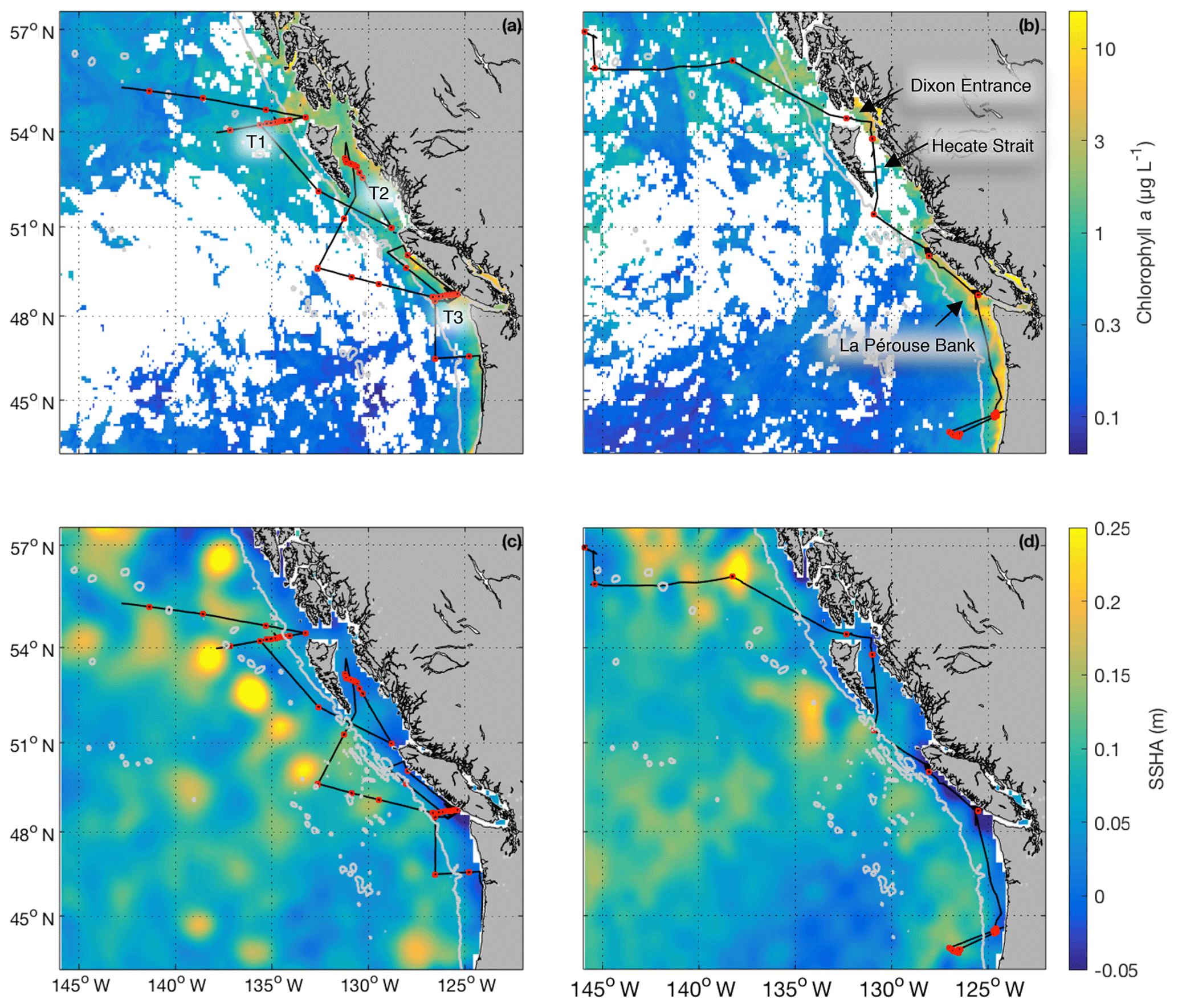
Figure 1Cruise tracks and discrete sampling stations (red circles) for the July 2016 (O16) cruise (a, c) and August 2017 (O17) cruise (b, d). Panels (a) and (b) show Chl a concentration (log scale) derived from Aqua MODIS satellite and averaged over the duration of the respective cruise. Panels (c) and (d) show average sea surface height anomaly (SSHA). Panel (a) shows the location of the T1–T3 transects surveyed during the 2016, whereas panel (b) shows the geographic locations of interest. The grey line represents the coastal–oceanic boundary, defined here as the 2000 m isobath.
High-resolution surface water DMS measurements were conducted using membrane inlet mass spectrometry (MIMS) following published methods (Tortell, 2005b; Nemcek et al., 2008). The MIMS system, sampling from the ship's underway seawater flow-through system (∼5 m intake depth), allows for high-frequency measurements (2–3 times a minute), yielding a spatial resolution of ∼150–200 m at normal ship speeds of 8–10 kn. During these cruises, DMS concentrations were also measured in discrete water samples collected at 5 m depth using a purge-and-trap system connected to a gas chromatograph equipped with a flame photometric detector (FPD-GC) (Kiene and Service, 1991). These discrete measurements were used to assess the accuracy of MIMS-based measurements. We found good agreement between methods, with a mean absolute error of 0.90 nM, root-mean-square error of 1.4 nM and coefficient of determination of r2=0.89 between the two instruments across the full range of measured concentrations (Fig. 3).
High-resolution DMS measurements were paired with rate measurements and ancillary underway data to examine potential drivers of spatial variation. A shipboard thermosalinograph was used to measure sea surface temperature (SST) and salinity at high spatial resolution (SBE 45 and SBE 38 for salinity and temperature, respectively). Chlorophyll a (Chl a) concentration was measured using a WET Labs ACS absorbance and attenuation meter, based on the absorption line height at 676 nm (Bricaud et al., 1995; Roesler and Barnard 2013; Burt et al., 2018). These Chl a concentrations were further used to derive an estimate of phytoplankton assemblage size structure and taxonomic distributions, based on the empirical algorithm of Hirata et al. (2011). Phytoplankton size-class estimates derived from this algorithm agreed well (r2>0.75) with discrete high-performance liquid chromatography (HPLC)-derived estimates (methods described below; Zeng et al., 2018). MIMS was also used to determine the ratio of oxygen and argon concentrations relative to atmospheric saturation. The resulting biological oxygen saturation term, ΔO2∕Ar, can be used to calculate net community productivity (NCP) from the air to sea gas exchange of O2 (Kaiser et al., 2005). We used the calculation approach of Reuer et al. (2007) to compute NCP from our ΔO2∕Ar measurements. We note that some of these estimates, particularly in regions of active upwelling, are likely negatively biased by the entrainment of O2-undersaturated water into the mixed layer. While this effect can be accounted for using N2O measurements (Izett et al., 2018), we do not have these data available for our cruises. Thus, our derived NCP estimates likely represent underestimates, and we have removed all negative NCP values. Nonetheless, the general spatial patterns we observed in NCP are likely to be robust.
2.2.2 Station-based measurements
We measured a suite of variables at selected sampling stations along the cruise track. All water for ancillary measurements was taken from 5 m depth, collected using Niskin bottles. A Sea-Bird CTD probe (Sea-Bird 911plus) was deployed at each station to obtain depth profiles of hydrographic features over the upper 200 m of the water column. A density difference criterion of 0.05 kg m−3 was used to calculate mixed-layer depths.
DMS loss and DMSP consumption rates were measured using the radio-labelled 35S methods outlined by Kiene and Linn (2000), with some modifications to minimize the release of DMSPd (dissolved DMSP) during incubations. Briefly, 35S-labelled DMSPd or DMS was added to samples at non-perturbing concentrations (< 1 % of ambient levels). Samples were incubated in the dark at surface water temperatures for < 1 h (35S-DMSP) or < 7 h (35S-DMS). The rate constant for DMSPd turnover was determined by measuring the disappearance of 35S-DMSP from the dissolved (< 0.2 µm) pool. The rate constants for DMS loss were determined by measuring the accumulation of dissolved, non-volatile 35S transformation products derived from the volatile 35S-DMS tracer. Consumption rates (nmol L−1 d−1) were calculated by multiplying in situ DMS or DMSPd concentrations by the measured rate constant (kDMS or kDMSPd, respectively).
Primary productivity was measured using 24 h 14C uptake incubations, following the method outlined by Schuback et al. (2015). Incubation bottles were held in a deck-board incubator plumbed with continuously flowing seawater to achieve in situ temperature. The light intensity was adjusted to ∼30 % surface irradiance enriched in blue light using neutral density screening in combination with blue photographic film (LEE filters: no. 209 and CT blue maximum transmission at approximately 460 nm). Light levels in the tank were measured with a ULM-500 light meter equipped with a 4π sensor (Walz). Bacterial production was measured using the tritiated leucine method (Smith and Azam, 1992) and converted to carbon units (Simon and Azam, 1989; Ducklow et al., 2000). Station samples were also analyzed for total and dissolved DMSP (DMSPt and DMSPd) with a GC-FPD discrete method using the previously described NaOH cleavage and small-volume gravity drip filtration method (Dacey and Blough, 1987; Kiene and Slezak, 2006). Particulate DMSP (DMSPp) was calculated by subtracting DMSPd from DMSPt (Zindler et al., 2012; Levine et al., 2016).
We obtained discrete estimates of phytoplankton assemblage composition using diagnostic pigment analysis (DPA) of photosynthetic pigments measured using HPLC. For these measurements, 1 L samples were collected on glass fiber filters (GF/F grade, nominal pore size ∼0.7 µm), flash frozen in liquid nitrogen and stored frozen until analysis at the NASA Goddard Space Flight Center Ocean Ecology Laboratory (Van Heukelem and Thomas, 2001). The DPA method was originally developed by Vidussi et al. (2001) and subsequently refined (Uitz et al., 2006; Hirata et al., 2008; Brewin et al., 2010) to more accurately capture phytoplankton type and size class. The estimation formulas used here are those of Hirata et al. (2011), with coefficients tuned specifically for the NESAP by Zeng et al. (2018). Percent contribution to phytoplankton assemblage was assessed for three size classes (micro-size, nano-size and pico-size).
2.3 Compilation of published data
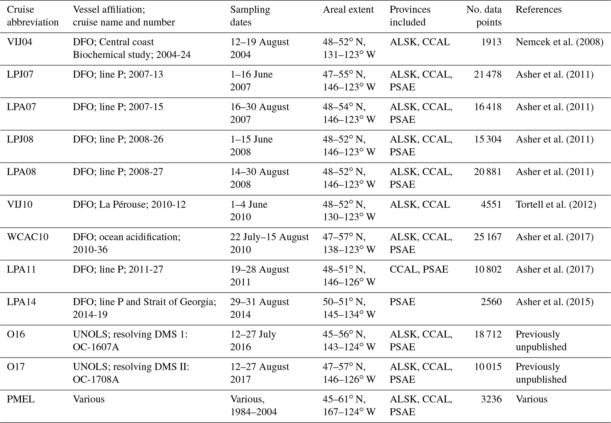
To provide a broader regional spatial context for our observations, we combined discrete DMS measurements from the PMEL data archive with high-spatial-resolution DMS measurements made using MIMS since the early 2000s. Table 1 provides dates and spatial domains of the cruises, along with relevant literature citations. Note that some of the DMS data included in this compilation have not been previously published. All of our compiled MIMS data have been made available on the PMEL database (https://saga.pmel.noaa.gov/dms/, last access: 26 February 2019).
Table 1Summary of DMS data included in this study. With the exception of the PMEL data, all measurements are derived from membrane inlet mass spectrometry (MIMS).
2.3.1 MIMS data sets
MIMS-based observations included in this study are derived from 11 cruises conducted between 2004 and 2017, primarily aboard the Canadian Coast Guard ship John P. Tully as part of ongoing time-series monitoring programs conducted by the Department of Fisheries and Oceans Canada (DFO). Only summertime data (defined here as June, July and August, JJA) falling within the NESAP region (44.5–61∘ N, 180–120∘ W) were included in this compilation. Although DMS concentrations and phytoplankton biomass often remain high through September (Galí et al., 2018; Lana et al., 2011; Steiner et al., 2012), there are fewer DMS data available for this month. Measurements were binned to a temporal sampling resolution of 1 min. All DMS data points are paired with shipboard sea surface salinity and SST. The cruises VIJ04, VIJ10, WCAC10, LPA11, O16 and O17 also include paired NCP estimates obtained from MIMS measurements, using the ΔO2∕Ar-based method described above.
2.3.2 PMEL data extraction
We accessed the PMEL database (http://saga.pmel.noaa.gov/dms/, last access: 6 December 2017) on 6 December 2017 to extract observations from June, July and August in the NESAP region defined above. Our selection criteria yielded 3236 data points between 1984 and 2003. These observations were relatively evenly distributed between the 3 months but were biased spatially, with a preponderance of data derived from on-shelf waters off the coast of Alaska (see Fig. 8b). As with MIMS data, the majority of data points in the PMEL database included paired sea surface salinity and SST measurements (94.6 % and 99.8 %, respectively).
2.4 Ancillary measurements
Ancillary oceanographic data were used to contextualize DMS spatial distributions, examine potential correlations to environmental variables and evaluate the performance of several empirical algorithms predicting DMS concentrations. In many cases, ancillary variables of interest (e.g. Chl a) were not reported in conjunction with DMS data, and thus we utilized a number of remote sensing data products, as described below. Remotely sensed parameters were linearly interpolated to the spatial resolution of ship-based DMS observations.
Aqua MODIS satellite data were used to obtain information on photosynthetically available radiation (PAR; Frouin et al., 2003), Chl a (OCI algorithm; O'Reilly et al., 1998; Hu et al., 2012), calcite (Gordon et al., 2001; Balch et al., 2005) and diffuse attenuation coefficients (Werdell and Bailey, 2005). For these data products, we extracted level 3 gridded data from http://oceancolor.gsfc.nasa.gov/cgi/l3, last access: 15 January 2018 at 9 km resolution. Monthly means for Chl a, calcite and kd were utilized to maximize spatial coverage by minimizing data gaps caused by cloudiness, whereas 8 d average PAR data were used. Aqua MODIS chlorophyll and sea surface temperature (SST) data were also used to estimate sea surface nitrate (SSN) using a North Pacific-specific algorithm (Goes et al., 2000). Aqua MODIS data are only available starting in July 2002, whereas most of the PMEL data set in this region is from sampling prior to 2003. For earlier observations (going back to 1997), we used Chl a data from the SeaWiFS satellite. Satellite Chl a, calcite and kd data were unavailable prior to 1997 (< 1 % of DMS data).
We obtained information on sea surface height anomalies (SSHAs) using gridded data sets (5 d, 0.17∘ × 0.17∘ resolution) obtained from ftp://podaac-ftp.jpl.nasa.gov/allData/merged_alt/L4/cdr_grid_interim, last access: 5 October 2017. This level 4 satellite product is derived from various sensors, and data are not available before 1992. Mixed-layer depths at a monthly 1∘ resolution were obtained from the China Second Institute of Oceanography (CSIO) ftp://data.argo.org.cn/pub/ARGO/BOA_Argo/, last access: 10 November 2017. These data are based on gridded Argo float data interpolated using the Barnes method and are available for the years 2004–2017 (Li et al., 2017). Due to limitations in Argo operational depths, data are largely absent from waters shallower than 2000 m (136 out of 249 1∘ × 1∘ bins).
We calculated sea–air DMS fluxes from DMS concentration data and surface wind speeds using the gas transfer parameterization of Sweeney et al. (2007) and the Schmidt number formulation of Saltzman et al. (1993). Wind speed data for flux calculations were obtained from the National Centers for Environmental Prediction/National Center for Atmospheric Research (NCEP/NCAR) reanalysis data set (https://www.esrl.noaa.gov/psd/data/gridded/data.ncep.reanalysis.pressure.html, last access: 4 October 2017) at a 2.5∘ daily resolution. These calculations were performed prior to data binning (described below) such that temporally resolved sea–air flux was calculated for all ∼150 000 DMS data points. Following previous studies, we assume negligible atmospheric DMS concentrations for our calculations, leading to a potential (though likely small) overestimate of the sea–air flux. For the purposes of comparison with fluxes, we calculated DMS column burden along transects by multiplying DMS concentration and average mixed-layer depth.
2.5 Data binning and province assignment
High-resolution underway measurements may introduce sampling biases due the large number of data points collected. For example, a ship holding station will increase spatial data density at a particular location, and the large number of observations can exert a disproportionate influence on derived mean values. To address this, all measurements in the data set were assigned to 1∘ spatial bins, in which all observations for a given year were averaged. All observations within the JJA months for a given year were averaged, rather than deriving separate monthly climatologies. The resulting yearly data grids were then averaged to create long-term gridded means. This technique effectively assigns equal weight to each year of measurements in a given grid cell. Both DMS and paired ancillary parameters were binned using this method.
Following the approach of L11, data grid cells were assigned to Longhurst Biogeochemical Provinces to examine patterns across different regimes within the greater NESAP (Longhurst, 2007). Three primary provinces fall within the domain of our study region: the California Upwelling Coastal Province (CCAL), Alaska Downwelling Coastal Province (ALSK) and Pacific subarctic Gyres Province – East (PSAE) (Fig. 8). The CCAL province, as defined by Longhurst, extends south to 16.5∘ N. Hereafter, all references to the CCAL refer to the portion of this province above 44.5∘ N. Province boundary designations were obtained from http://www.marineregions.org/downloads.php (last access: 17 October 2017), and the MATLAB native inpolygon.m function was used to assign grid cells to individual provinces. Any grid cell either inside or on the edge of boundaries was assigned to a particular province. As such, some data cells (37 out of 249 total) are assigned to multiple provinces. Average summer DMS concentrations and flux measurements were computed for each province. For comparison to L11, we recalculated the average summertime DMS concentration and flux in the three study provinces using only the PMEL data utilized by L11. The PMEL data were first binned using the year-weighted method described above.
2.6 Statistical analysis and empirical algorithms
We used our compiled data set to examine broadscale relationships between DMS and other oceanographic variables. For this analysis, data were log-transformed to overcome non-normal distributions, and the strength of pairwise relationships was assessed by computing Pearson's correlation coefficients. Correlations were applied to 1∘ × 1∘ binned data both within individual provinces and across the entire NESAP.
We also used several existing empirical algorithms to reconstruct DMS fields at a 1∘ × 1∘ resolution from various environmental predictor variables, comparing the accuracy of the resultant products against our binned DMS observations. The algorithms tested in this study include those of Simó and Dachs (2002), Vallina and Simó (2007), Watanabe et al. (2007), and Galí et al. (2018) (hereafter, SD02, VS07, W07 and G18, respectively). Both SD02 and VS07 used global databases to develop their algorithms. SD02 relates DMS to Chl a : MLD, with Chl a values > 15 µg L−1 removed prior to analysis. VS07 relates DMS concentration to solar radiative dose (SRD). This term, as defined by the authors, is based on light extinction coefficients (kd), sea surface irradiance (I0) and mixed-layer depth. Due to the large areal extent of the study area, we used Aqua MODIS-derived PAR in lieu of the station-based I0 measurements used by the authors. Similarly, strong variation in kd in coastal vs. open ocean waters is expected. We thus modified the author's approach and used satellite-derived kd (based on a chlorophyll-dependent algorithm; Werdell and Bailey, 2005) rather than a fixed coefficient. W07 use data specific to the North Pacific and relates DMS to SST, SSN and latitude. The two-step G18 algorithm utilizes a previously developed DMSPt predictive algorithm based on Chl a and MLD (Galí et al., 2015) in conjunction with PAR measurements. In order to test this algorithm, we utilized the satellite-derived PAR, MLD and Chl a, described above. We further modify the author's approach by testing performance on our 1∘ × 1∘ binned data, rather than data binned at 5∘ × 5∘, in order to maximize the number of observations. Recognizing the utility of re-parameterizing proposed algorithms for specific areas, we tested algorithms using both published linear coefficients and coefficients derived specifically for the NESAP using a least-squares approach to determine the best fit to our data set. The coefficients used to test the original G18 were those regionally tuned by the authors for latitudes above 45∘ N.

Figure 2Spatial distribution of DMS (a), salinity (b), net community production (c – log scale), and microphytoplankton, nanophytoplankton, and picophytoplankton relative abundance (d–f) during the O16 cruise (July 2016) and the O17 cruise (August 2017). Colour scaling on the maps is adjusted to ensure readability and best illustrate spatial patterns. Some data values are higher than the maximum scale of the colour bar. The inset box shows the La Pérouse Bank region, as marked by the red circle. The grey line represents the coastal–open ocean boundary (2000 m isobath).
We begin by presenting an overview of our new DMS measurements and ancillary data from the 2016 to 2017 summer cruises, highlighting DMS distributions and the presence of distinct surface water properties across different parts of our transect. We then provide a detailed description of DMS dynamics across several hydrographic frontal zones, discussing the potential role of various processes in driving these gradients. Finally, we present an updated summertime climatology for this region, compiling our new measurements with existing DMS observations from across the NESAP to examine large-scale patterns in DMS distributions and correlations with other oceanographic variables. The potential role of these variables in driving DMS distributions in the NESAP and the need for additional process studies are addressed in the discussion.
3.1 Oceanographic conditions in the NESAP during summer 2016–2017
Our 2016 and 2017 cruises surveyed oceanographic regimes from offshore HNLC regions to productive coastal upwelling zones. As indicated by Aqua MODIS satellite imagery, Chl a concentrations exhibited strong gradients across the oceanic–coastal transition in both 2016 and 2017 (Fig. 1). Coastal waters showed elevated Chl a, with maximum values of 50 and 18 µg L−1 in 2016 and 2017, respectively. In both years, the highest Chl a values were observed in waters with shallow mixed-layer depths (< 10 m) along the La Pérouse Bank (Fig. 1). In the off-shelf regions, Chl a concentrations appeared uniformly low in 2016, although significant cloud cover limited the availability of satellite imagery. By comparison, we observed generally higher Chl a concentrations in offshore waters in 2017. Most notably, our cruise track passed through an apparent coccolithophore bloom in the northern Gulf of Alaska, where a large calcite signal (∼2 mmol PIC m−3) was detected in Aqua MODIS imagery. Patterns in NCP were generally similar to those of Chl a, with elevated production in coastal waters (Fig. 2c). In both years, we observed NCP on La Pérouse Bank exceeding 100 mmol O2 m−2 d−1 (Fig. 2c, inset).
Coastal regions exhibited generally fresher surface waters and shallower mixed-layer depths, except for several regions of enhanced vertical mixing associated with upwelling. This coastal upwelling signature was apparent in the elevated salinity and decreased temperature of surface waters and also through the presence of negative sea surface height anomalies (Fig. 1c, d). Small-scale regional heterogeneity in coastal regions was apparent in both years, with salinity and temperature exhibiting sharp gradients over the continental shelf, associated with riverine input and complex mixing processes. By comparison, oceanic surface waters showed less spatial heterogeneity and were generally more saline, with deeper mixed-layers (Fig. 2b). The sea surface height anomaly field indicated the presence of several Sitka and Haida eddies in both years (Fig. 1c, d), enhancing mesoscale variability through the transport of coastal water offshore.
Using the approach of Hirata et al. (2011) and Zeng et al. (2018), we derived high-resolution estimates of phytoplankton assemblage composition from our underway Chl a measurements. This approach revealed a predominance of phytoplankton in the micro-size class (> 20 µm) in coastal waters (Fig. 2d), with an average of 50 % of Chl a attributable to microphytoplankton. In contrast, off-shelf waters showed greater diversity in phytoplankton composition. In these waters, microphytoplankton accounted for ∼25 % of total Chl a, while the pico-size and nano-size classes accounted for ∼30 % and ∼40 %, respectively (Fig. 2e, f).
3.2 DMS distributions
Across our study region, surface water DMS concentrations ranged from < 1 to 24 nM in 2016 and < 1 to 18 nM in 2017 (Figs. 2a and 3). We observed a number of localized DMS “hotspots” in regions of elevated Chl a and NCP. In both years, these localized high-DMS regions were particularly evident in the vicinity of the highly productive La Pérouse Bank (Fig. 2a, inset). We also observed several areas where strong DMS gradients co-occurred with salinity fronts. These areas include the T1–T3 transects surveyed in O16, detailed below. Despite associations between DMS concentration and several variables in some localized regions, we only observed weak correlations between DMS and other measured variables across the full cruise tracks. During O16, DMS concentrations were most strongly correlated to NCP, with a Pearson's coefficient of r=0.42 (p < 0.001). This relationship was substantially weaker in O17 (r=0.29; p < 0.001).

Figure 3DMS concentrations during the O16 cruise in July 2016 (a) and the O17 cruise in August 2017 (b), as measured by membrane inlet mass spectrometry (MIMS, continuous black line) and a purge-and-trap sampling system connected to a gas chromatograph equipped with a flame photometric detector (grey symbols). Mean absolute error was 0.93 nM and root-mean-square error was 1.4 nM for all paired measurements between the two instruments. A linear regression of the two data sets yields a coefficient of determination of r2=0.89.
3.3 Detailed surveys of DMS across hydrographic frontal zones
During the O16 cruise, we sampled along three repeated transects to map DMS distributions near hydrographic frontal zones. All three transects showed significant gradients in salinity, Chl a and DMS and DMSP concentrations, as well as in the metabolic activity of phytoplankton and bacteria (Figs. 4 and 6–7). While DMS concentrations appeared to co-vary with salinity and Chl a across these frontal zones, the strength and direction of these relationships were not consistent across the three transects. We discuss each transect in detail below.

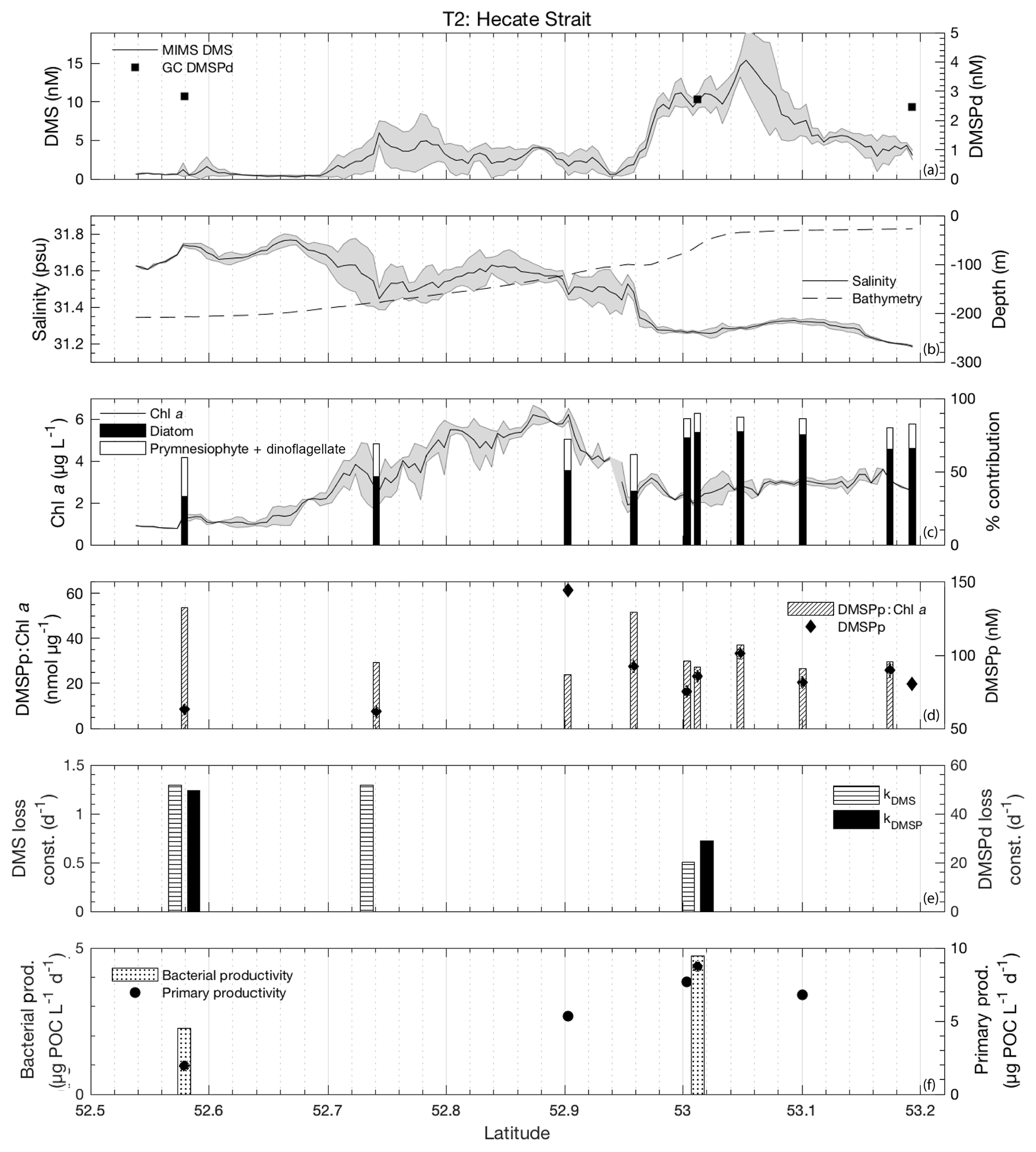
Figure 4MIMS-based DMS concentration measurements and station-based DMSPd measurements (a), salinity and bathymetry (b), Chl a and HPLC-based station estimates of diatom and prymnesiophyte as defined percentage contribution to total assemblage (c), DMSPp concentrations and DMSPp : Chl a ratios (d), DMS and DMSP consumption rate constants (e), and bacterial and primary productivity rates (f) along the T1 transect west of Dixon Entrance during July 2016 (O16 cruise). Shaded regions represent a standard deviation of repeated measurements across the transect. The vertical dotted line in panel (b) indicates the approximate shelf break (2000 m) at 134.4∘ W.
3.3.1 Transect 1
T1 was located west of Dixon Entrance (Fig. 1) in waters influenced by the Alaska Current and coastal water masses. Offshore waters along this transect were more saline and colder than those on the shelf. The area exhibited DMS concentrations up to 10 nM in off-shelf, saline waters (Fig. 4). Particulate and dissolved DMSP ranged from ∼60 to 125 and ∼1.8–4.7 nM, respectively, and showed no significant correlation to DMS (Fig. 4d). At the shelf break (approx. 134.4∘ W, indicated on Fig. 4 by dotted line), we measured a sharp drop in salinity and corresponding decrease in DMS concentrations, with concentrations remaining below ∼3 nM over the most coastal parts of the transect. Across the entire T1 transect, DMS concentrations displayed a striking fine-scale coherence to salinity (r=0.80; p < 0.001; Fig. 4a, b). A significant positive correlation was also observed with SSHA (r=0.51; p < 0.001), indicating a potential influence of westward-propagating Haida eddies. Figure 5 shows a line plot of SSHA measurements from the approximate time of T1 sampling, overlaid by DMS concentrations. The coherence between DMS concentrations and mesoscale oceanographic features can be seen in this figure despite differences in the spatial resolution of the two data sets.
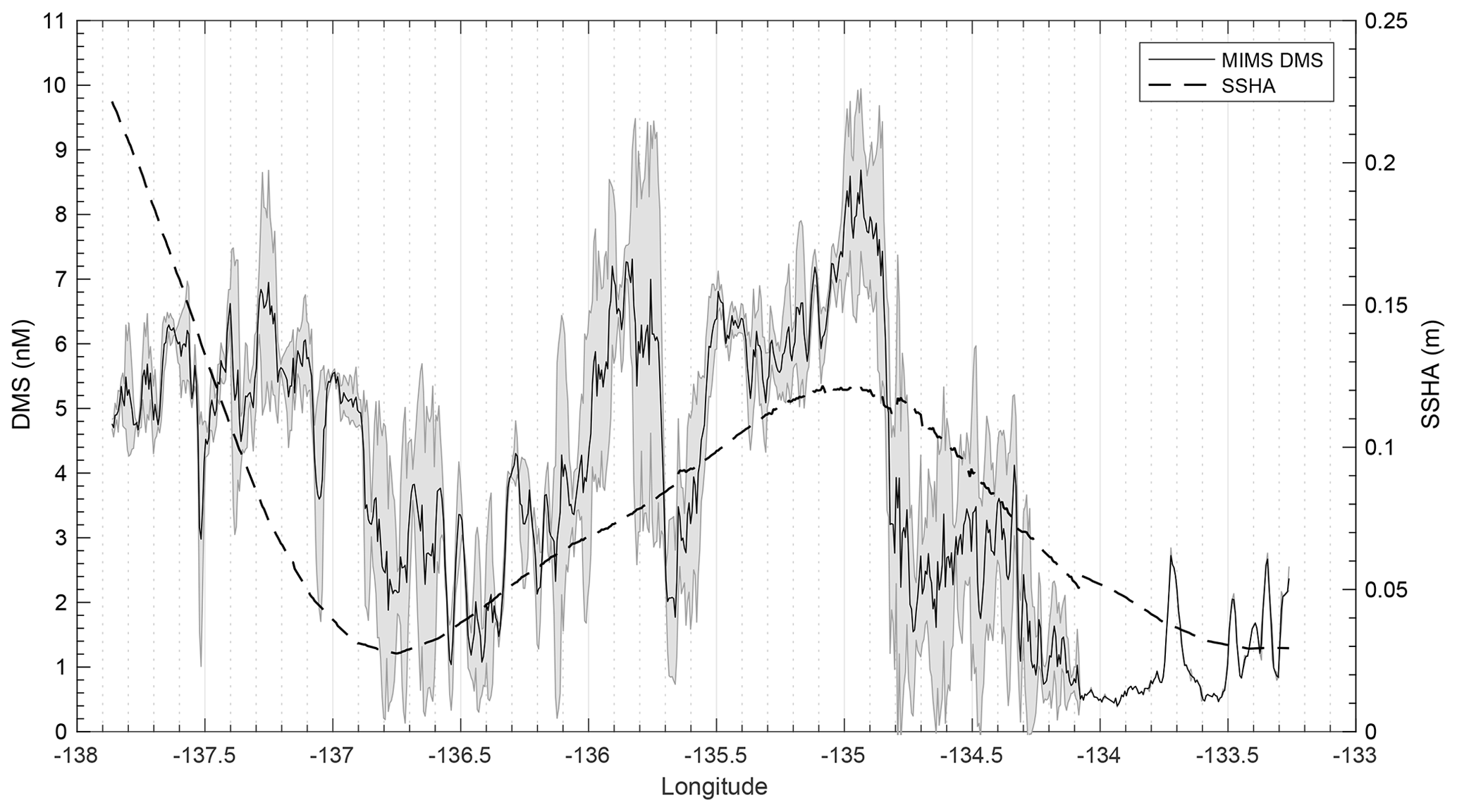
Figure 5Line plot of sea surface height anomaly (SSHA) on 15 July 2016 and observed DMS concentrations between 14 and 16 July 2016 along T1. DMS along the T1 transect is highest in those areas influenced by positive SSHA values.
The lower-salinity coastal waters along T1 were characterized by elevated Chl a concentrations (Fig. 4c), resulting in a negative correlation between DMS concentrations and chlorophyll (; p < 0.001). Figure 4c shows the estimated percent abundance of diatoms and combined dinoflagellates and prymnesiophytes as derived from HPLC-based DPA analysis. The remaining phytoplankton assemblage consisted largely of picoeukaryotes (13 %–36 %). Although HPLC samples are not available for all of the coastal waters we sampled, results obtained from the empirical algorithm of Hirata et al. (2011) using underway absorption data suggest a shift in phytoplankton assemblage composition from smaller size classes in offshore waters to a microphytoplankton-dominated community in on-shelf waters. DMS exhibited relatively weak, though statistically significant (p < 0.001), positive correlations with the algorithm-derived relative abundance of nanophytoplankton and picophytoplankton size classes (r=0.55 and r=0.38, respectively) and a negative correlation with the relative abundance of microphytoplankton (). In support of this result, discrete HPLC measurements revealed a strong positive relationship between DMS concentration and the combined relative abundance of prymnesiophytes and dinoflagellates (r=0.89; p=0.001) and a negative correlation to diatom abundance (; p=0.036). We also observed a strong positive correlation between DMS and DMSPp : Chl a (r=0.80; p=0.003) suggesting higher cellular DMSP concentrations in phytoplankton assemblages in the off-shelf regions of this transect. Overall, results from this transect demonstrate a transition from high-DMS concentrations in the lower-productivity, nanophytoplankton-dominated offshore waters to low-DMS concentrations in the higher-productivity, diatom-dominated nearshore region.
Average rate constants (d−1) for biological consumption of DMS and DMSPd appeared qualitatively higher in the on-shelf region (although insufficient sampling does not allow for reliable statistical testing), suggesting faster removal of DMS and DMSP from coastal surface waters with lower DMS concentrations. For DMS and DMSPd, respectively, loss constants averaged 1.15±0.3 and 88.2±13.9 d−1 onshore, as compared to 0.66±0.045 and 39.6±1.45 d−1 in offshore stations (Fig. 4e). Net primary productivity and bacterial productivity also showed a qualitative trend towards higher average values in the low-DMS coastal waters, but these differences were not statistically significant. Although biological loss of DMS constitutes only one of several loss terms, the patterns observed here suggest that enhanced microbial activity and relatively higher DMS and DMSP consumption rate constants played a role in maintaining lower concentrations of these compounds in nearshore waters.
We calculated the mixed-layer DMS burden by multiplying concentration and average mixed-layer depth (13 m). Biological DMS loss integrated over the mixed layer averaged 22 µmol m−2 d−1, sufficient for daily removal of 47 % of the DMS burden. By comparison, derived sea–air flux estimates across the transect exhibited a mean value of 13 µmol DMS m−2 d−1, accounting for ∼25 % of the mixed-layer DMS burden daily. Due to a relatively homogenous wind field over the area of our sampling transect, the sea–air fluxes were tightly correlated to DMS concentrations such that the lower DMS concentrations in nearshore regions cannot be explained by greater rates of ventilation to the atmosphere.
3.3.2 Transect 2
The second sampling transect, T2, was located in the coastal waters of Hecate Strait situated on the continental shelf (Fig. 1). Sea surface temperatures along this transect exhibited low variability (standard deviation ∼0.5 ∘C), with the coldest waters located mid-transect in areas of highest Chl a. Mixed-layer depths ranged from 10 to 15 m, and DMS concentrations ranged from < 0.5 nM to nearly 20 nM (Fig. 6). DMSPd concentrations exhibited only minor variations over the transect (2.5–2.8 nM), while DMSPp concentrations showed greater variability (61–144 nM). Neither DMSPd nor DMSPp was correlated to DMS concentrations. HPLC measurements suggested that diatoms dominated across the entire transect and particularly in northern regions (Fig. 6c). Picoeukaryotes and green algae comprised the bulk of the remaining phytoplankton assemblage composition (generally < 10 %). In contrast to our observations for T1, DMS concentrations exhibited negative correlations to both salinity (; p < 0.001; Fig. 6b) and SSHA (; p < 0.001) in this area and were not significantly correlated to Chl a (Fig. 6c). Despite the lack of correlation to Chl a, DMS did exhibit significant, though weak, positive correlations with estimates of relative microphytoplankton abundance (r=0.22; p < 0.001) and stronger negative correlations with the abundance of pico-size and nano-size classes (T2: ; ; p < 0.001; Fig. 6c). In support of this observation, HPLC-pigment data from discrete sampling stations revealed a strong positive relationship between DMS concentration and relative abundance of diatoms (r=0.88; p=0.001), and a negative correlation between DMS and combined dinoflagellate and prymnesiophyte abundance (; p=0.001). These correlations suggest diatoms as an important source of DMS, in contrast to that observed for T1.
Unlike bulk Chl a concentrations, we found that primary productivity showed a strong positive correlation with DMS along T2 (r=0.90; p=0.037), although this result is based on only four data points. Bacterial productivity was also significantly higher in the high-DMS waters, although this variable was even more sparsely sampled along the transect, and we cannot infer any meaningful statistical association with DMS (Fig. 6f). As with T1, both kDMSPd and kDMS appeared higher in the low-DMS portions of the transect. Across the entire transect, DMS and DMSP consumption rate constants ranged from 0.51 to 1.29 and 28.8 to 49.5 d−1, respectively (Fig. 6e). This result suggests microbial consumption as a potential driver of DMS distributions, with higher DMS and DMSP consumption rate constants in waters with lower DMS concentrations.
Integrated biological DMS loss was significantly higher than that of T1, with an average 78 µmol m−2 d−1 (equivalent to removal of 87 % of the DMS burden per day). By comparison, DMS sea–air flux across the transect was low, with a mean value of 2.9 µmol m−2 d−1. This flux was sufficient to remove only ∼6 % of mixed-layer DMS burden daily. We thus conclude that biological processes play a significant role in DMS turnover along this transect.
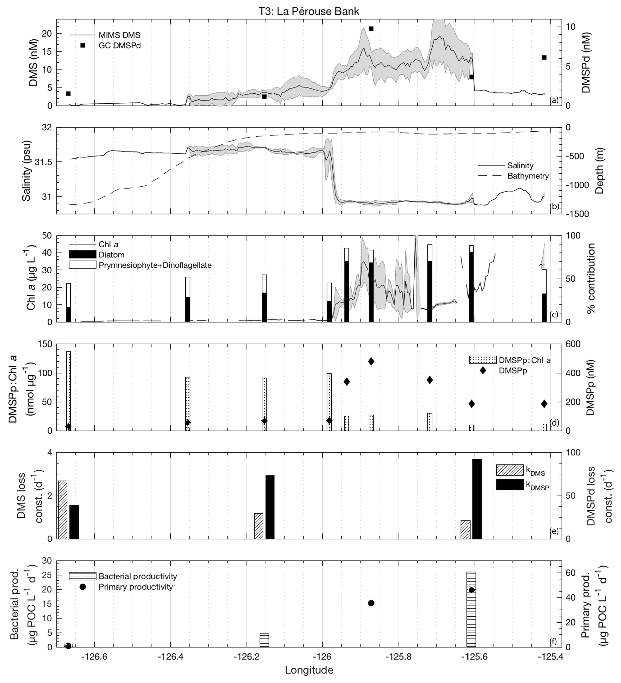
3.3.3 Transect 3
T3 was located in the highly productive coastal waters of La Pérouse Bank, along the continental shelf of the west coast of Vancouver Island (Fig. 1). DMS concentrations across this transect ranged from < 1 to 24 nM, while DMSPd and DMSPp concentrations were among the highest observed cruise-wide (1.1–9.8 and 26–480 nM, respectively; Fig. 7d). DMSPp was correlated to DMS (r=0.76; p=0.02). Mixed-layer depths ranged from 8 to 12 m, with the shallowest values found in fresher, salinity-stratified inshore waters influenced by riverine input. Sea surface temperature was lower in these low-salinity waters, although it varied little over the transect (standard deviation < 1 ∘C). With respect to other measured variables, DMS behaved in a similar way to the coastal T2 transect (Fig. 7a). We observed negative correlations between DMS and salinity (; p < 0.001; Fig. 7b) and SSHA (; p < 0.001). We also found elevated Chl a in the low-salinity waters, although there was only a weak positive correlation between Chl a and DMS (r=0.25; p < 0.001) across the full transect (Fig. 7c).
Microphytoplankton consisting primarily of diatoms dominated the low-salinity, high-DMS waters of the transect, with a shift towards smaller cells observed in the more saline waters farther offshore (Fig. 7c). Among the T3 stations, green algae, prokaryotes and picoeukaryotes each comprised ∼5 %–20 % of phytoplankton abundance. Similar to T2, we found a significant positive correlation between DMS and microphytoplankton (r=0.90; p < 0.001) and a negative correlation between DMS and phytoplankton of the nano-size and pico-size class (; ; p < 0.001). In support of this observation, HPLC-pigment data showed a strong positive relationship between DMS concentration and relative abundance of diatoms (r=0.94; p < 0.001) and a negative correlation with combined dinoflagellate and prymnesiophyte abundance (; p=0.023). A negative relationship was also observed between DMSPp : Chl a and DMS (; p=0.002) (Fig. 7d). In contrast to T1, high DMS coincided with regions of lower cellular DMSP concentrations among phytoplankton, consistent with the dominance of diatoms in the high-DMS portions of this transect.
Along the T3 transect, DMS exhibited a positive qualitative association with primary productivity and bacterial productivity, though these relationships are based on very few sampling points. It is noteworthy that the bacterial productivity measured along T3 was higher than anywhere else along the cruise track, with production more than 5-fold greater than the cruise-wide average. Values of kDMS ranged from 0.8 to 2.7 d−1 across the transect. As with T1 and T2, kDMS was higher in low-DMS regions of T3. In contrast, kDMSPd values along T3 increased in parallel with DMS concentrations (higher rate constants in higher DMS waters). DMSP loss constants ranged from 38.6 to 92.1 d−1 (Fig. 7e). The highest DMSP loss constant translates into a derived turnover time of just 16 min and coincided with the highest bacterial productivity (∼26 µg POC L−1 d−1).
Biological DMS loss integrated over the mixed layer was sufficiently high enough to remove > 100 % of the DMS burden daily (∼47 µmol m−2 d−1). By comparison, sea–air fluxes were a minor loss term (4.9 µmol m−2 d−1) and were sufficient to remove only ∼12 % of the mixed-layer DMS burden. Due to low removal rates and relative homogeneity of wind speed fields, sea–air flux cannot be invoked to explain the spatial distribution of DMS across this transect.
3.4 Regional DMS distribution – comparisons of 2016 and 2017 observations with past studies
To explore potential regional-scale relationships between DMS concentrations and other environmental variables, we combined our new DMS data with measurements collected over the past 3 decades, including previously unpublished high-resolution MIMS data. The addition of new measurements to the existing PMEL data set substantially increases spatial and temporal coverage in the NESAP. When data were binned to 1∘ × 1∘ resolution, coverage was increased by ∼20 % in the CCAL and ALSK Longhurst provinces and 14 % in the PSAE, with the overall addition of 90 data-containing grid cells (Table 2). As shown in Fig. 8, our measurements primarily increase data coverage in waters below 57∘ N. These regions were previously under-sampled in the PMEL data set utilized by L11, which was strongly biased to measurements near the coast of Alaska. Figure 9a further illustrates the latitudinal shift in data coverage with the inclusion of additional MIMS data. As shown in Fig. 9b, average derived DMS concentrations across latitudinal bands at the north and south extremes of our study area remain similar to those derived from the PMEL data set utilized by L11. However, in the region between 50 and 54∘ N, where there were few observations in the PMEL database, our compiled data show mean concentrations as much as 4.5 nM (∼40 %) lower than those calculated using PMEL data alone.
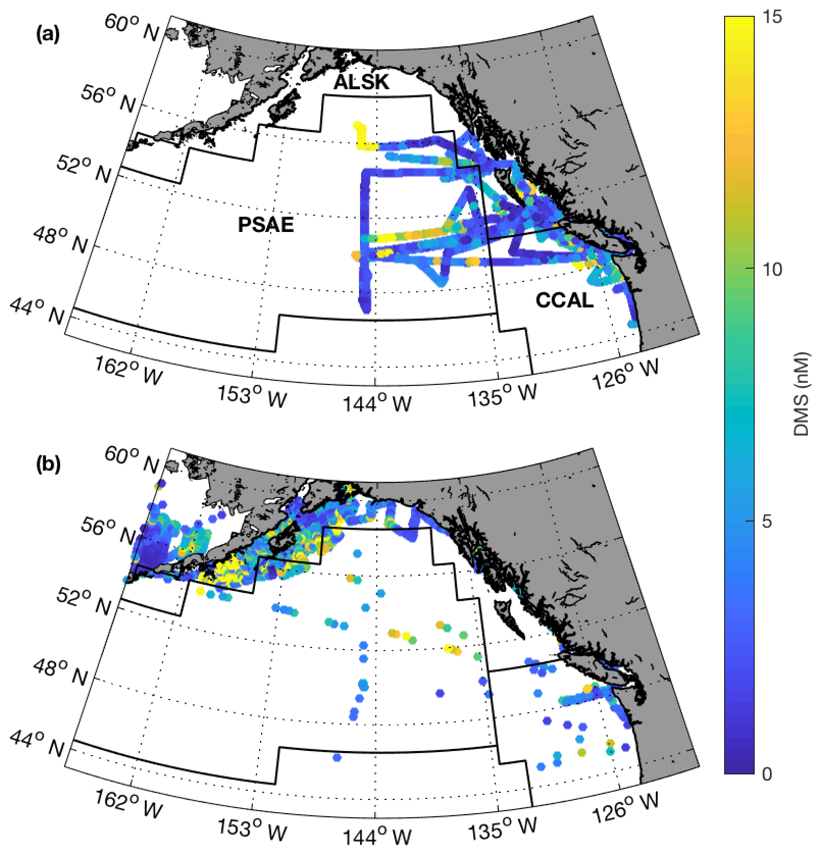
Figure 8Spatial distribution of summertime DMS measurements from MIMS (a; 2004–2017) and the PMEL (b; 1984–2004) data set. Black lines represent boundaries of the Longhurst biogeographical provinces, with province names shown in panel (a).
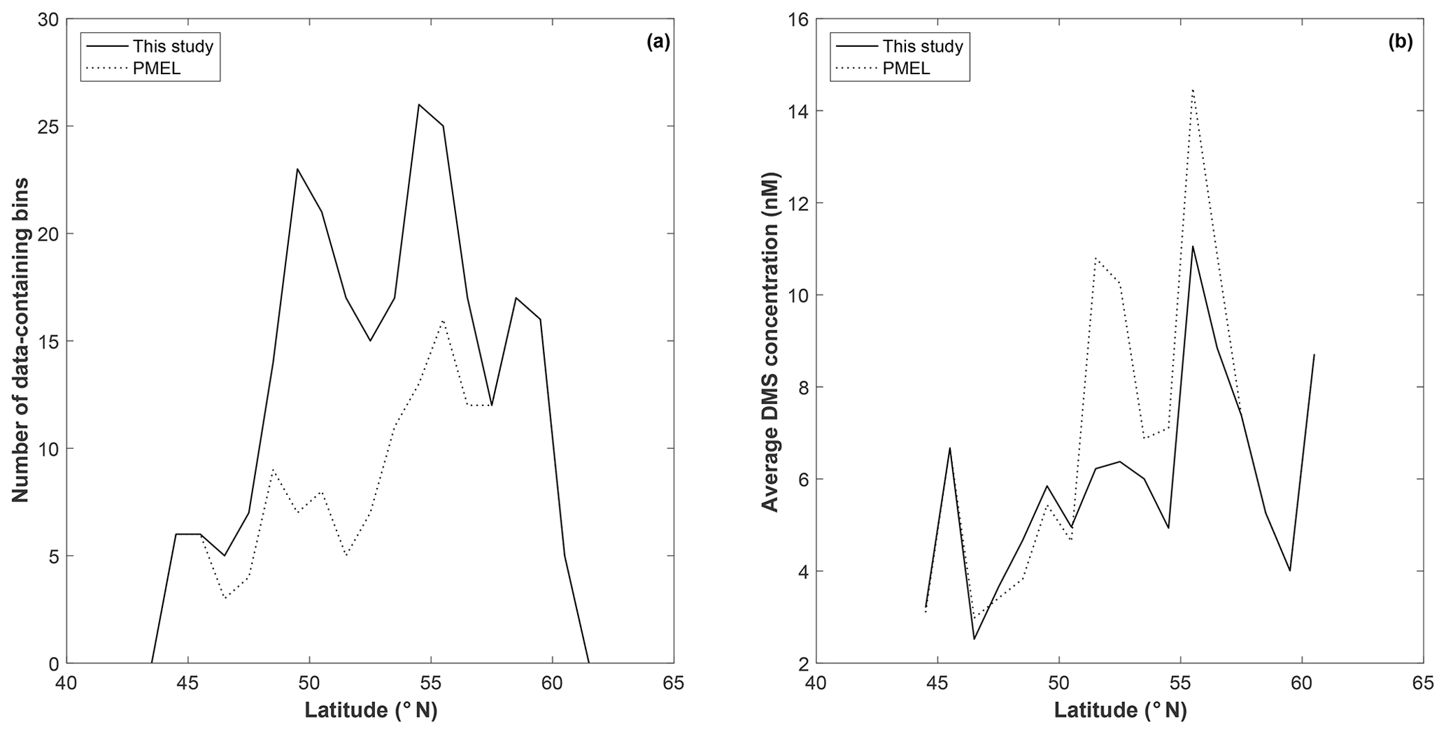
Figure 9Latitudinal distribution of data-containing bins (a) and average DMS concentration (b) for PMEL (dotted line) and combined (PMEL and MIMS) data sets.
Table 2Summertime DMS data coverage across the NESAP region and within Longhurst provinces. Values indicate the number of data-containing 1∘ × 1∘ spatial bins out of the total number of bins within the given area (denoted by a slash), with percent coverage of area shown in parentheses. The left column represents the coverage for the PMEL data set (as utilized by L11), and the right column represents the updated data set containing both PMEL measurements and MIM-based DMS concentration measurements.
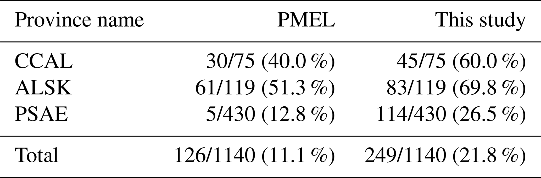
Table 3Mean DMS concentrations, sea–air fluxes and total summertime DMS flux for the PMEL data set utilized by L11 and the updated databases used in this study.
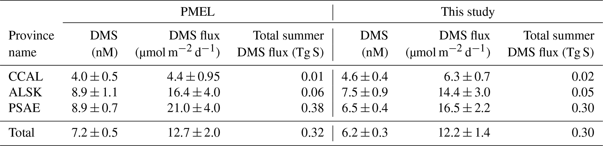
Table 3 shows the change in province-wide average DMS concentration, sea–air fluxes and total summertime DMS flux based on our updated analysis. Relative to our revised estimates, DMS concentrations and sea–air fluxes derived using only the PMEL data were lower in the CCAL and higher in both the PSAE and ALSK provinces. The most pronounced difference was that of sea–air flux in the PSAE, where estimated values decreased by 4.5 µmol m−2 d−1 (20 %). Despite these regional differences, the total summer DMS flux across the NESAP differed by only 6.5 % between our compiled data set (0.30 Tg S) and the PMEL data set utilized by L11 (0.32 Tg S).
Our compiled data set provides greater confidence in DMS concentrations and sea–air fluxes across the NESAP and enables us to better constrain spatial patterns. Figure 10 shows binned average summertime DMS concentration across the region as well as the derived sea–air DMS fluxes. The highest concentrations were observed in ALSK, where coastal waters contain maximum DMS concentrations exceeding 20 nM. A persistent region of elevated DMS concentrations was also evident in mid-PSAE oceanic region, with concentrations greater than 10 nM. Sea–air DMS fluxes showed a spatial distribution similar to DMS concentrations, with maximum values of > 100 µmol m−2 d−1. Calculated DMS : Chl a ratios for binned data (Fig. 10c) generally showed higher values in offshore NESAP waters.

Figure 10Summertime DMS concentrations (a), DMS sea–air fluxes (b) and DMS : Chl a ratios (c) binned to 1∘ × 1∘ spatial resolution. These maps were derived using our combined PMEL–MIMS data set (1984–2017; June, July and August). Black lines correspond to boundaries of Longhurst biogeochemical provinces (see Fig. 8 for province names). Maximum values (47 nM, 180 µmol m−2 d−1 and 47 nmol µg−1 for panels a, b and c, respectively) exceed the bounds of the colour bars. Maximum values for DMS and DMS flux occur in the waters south of the Alaska Peninsula, whereas maximum DMS : Chl a occurs mid-PSAE.
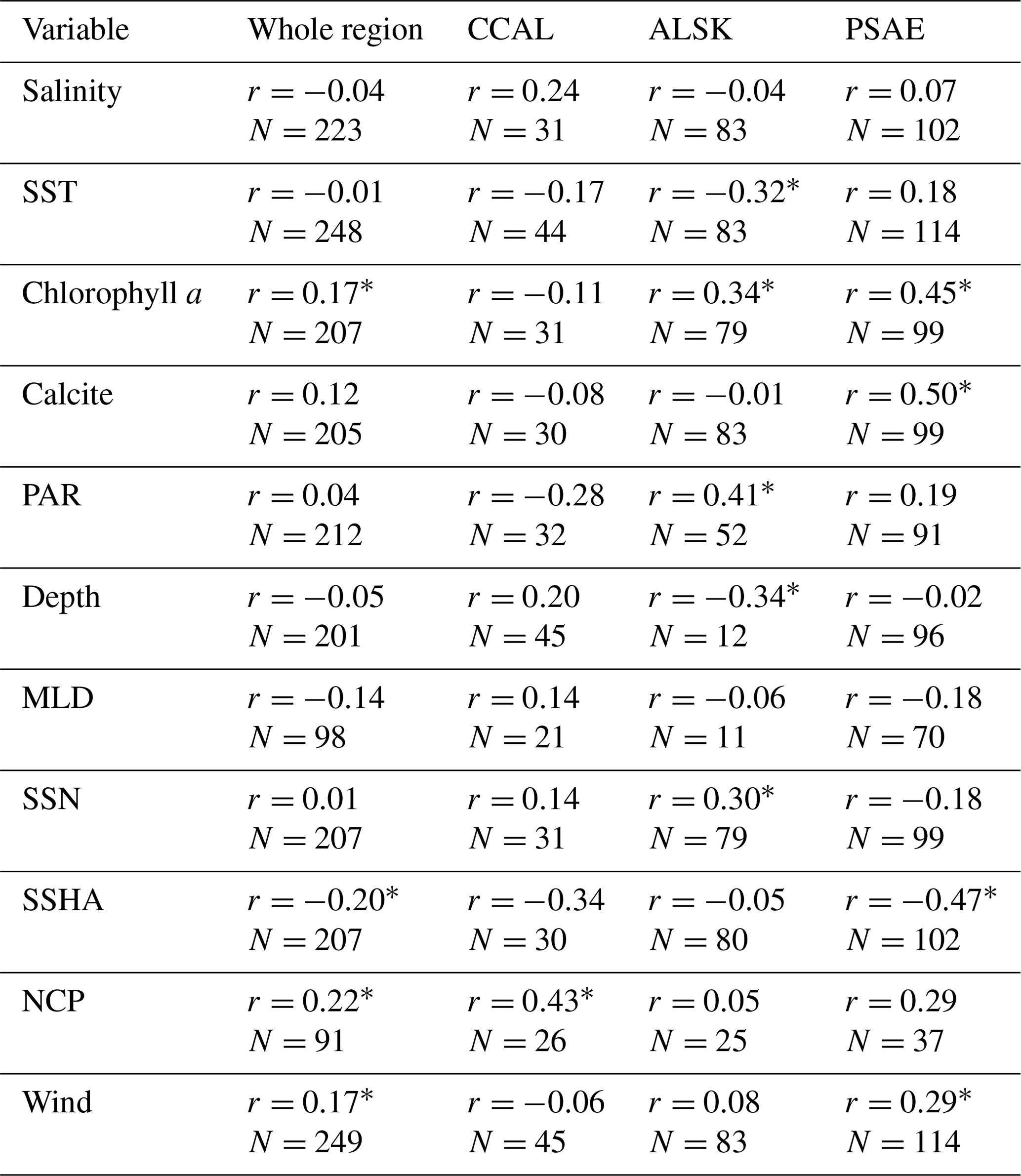
Table 4Pearson's correlation coefficients between DMS concentrations and other oceanographic variables binned to 1∘ spatial resolution. DMS data were derived from our combined PMEL and MIMS data set, variables are derived from in situ and satellite-based data. N represents the number of data pairs available for each correlation calculation (* indicates significance of p < 0.05).
3.5 Correlations and algorithm testing
Using our new data compilation, we examined the relationship between DMS concentrations and a suite of oceanographic variables across the NESAP. Table 4 shows both NESAP-wide and province-specific correlations derived from this analysis. While many correlations are weak or not statistically significant, some patterns do emerge, particularly in the offshore waters of the PSAE domain. No single variable explains a large portion of the DMS variation in this province, but statistically significant correlations exist between DMS, Chl a and calcite (r=0.45 and r=0.50, respectively). We also found a negative relationship between DMS and SSHA (). For the ALSK province, we found weak inverse correlations between DMS, SST () and water depth (). We observed positive correlations between DMS and derived surface NO3 concentrations, PAR and Chl a (r=0.30, 0.41 and 0.34, respectively). In contrast to other provinces, we observed a statistically significant correlation between DMS and NCP in the CCAL province (r=0.43). The lack of other significant correlations in the province may, in part, reflect the lower number of data points obtained for this region.
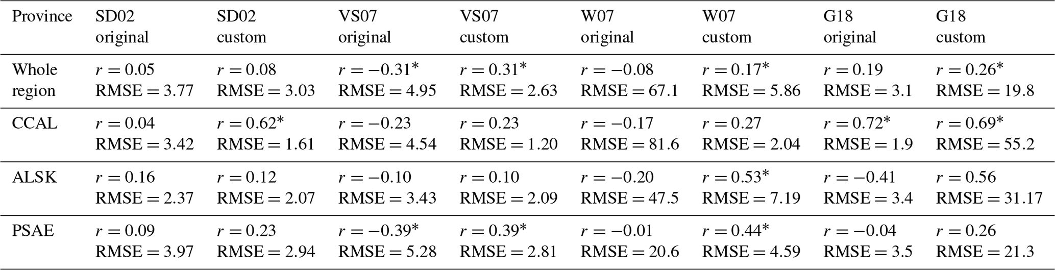
Moving beyond simple pairwise correlations, multivariate empirical algorithms provide an additional approach to assess the potential drivers of regional DMS dynamics. We evaluated the ability of five previously published algorithms to reproduce patterns in the DMS observations. In order to obtain the best possible results, we modified the original equations using a least-squares method to obtain the best-fit coefficients for our data set. We evaluated the algorithm outputs against observations using Pearson's correlation coefficients and root-mean-square errors (RMSEs). As shown in Table 5, model performance was generally low, with most correlation coefficients less than 0.53 and RMSE values ranging from 1.2 to 81.6 nM. The best results were obtained for the CCAL province, where both the tuned SD02 and the original G18 algorithms were able to predict DMS concentrations with moderate success (r=0.62, RMSE = 1.61 and r=0.72, RMSE = 1.9, for SD02 and G18, respectively). As both of these algorithms rely on MLD, which is only available for waters deeper than 2000 m, it is important to note that predictive strength can only be assessed for these off-shelf waters and should not be taken to represent performance in coastal waters. The customized VS07 (with coefficients tuned to the NESAP data) showed the best overall performance across the entire NESAP region. Yet, even this model showed only weak correlation between predicted and observed DMS values (r=0.31). Notably, the original linear coefficients for this model yielded DMS concentrations that were inversely correlated to the measured values. In no case did models using original linear coefficients outperform those using recalculated coefficients.
The results presented here provide new information on the fine-scale and regional patterns of DMS distributions across the NESAP. Our shipboard observations document sub-mesoscale variability in DMS concentration across hydrographic frontal zones, with associated process measurements providing insight into potential driving factors. By combining these new data with more than 3 decades of DMS measurements, we are able to improve data coverage for the NESAP to examine larger-scale spatial patterns and provide a more robust regional climatology to evaluate empirical predictive algorithms.
4.1 Contrasting cycling regimes within the NESAP
A number of studies have documented differences in DMS dynamics across oceanographic regimes in the NESAP (Royer et al., 2010; Asher et al., 2011, 2017). These regional differences result from complex ecosystem and environmental interactions and limit broadscale prediction of DMS concentrations and sea–air fluxes (Galí et al., 2018). Taxonomic composition of phytoplankton assemblages has been identified as a main driver of DMS distribution patterns. For example, dinoflagellates and prymnesiophytes typically have elevated DMS production, associated with greater intracellular concentrations of DMSP (Keller, 1989) and, in some cases, high activity of DMSP lyase (the enzyme that cleaves DMSP to DMS and acrylate; Steinke et al., 2002; Wolfe et al., 2002; Curson et al., 2018). In contrast, bloom-forming diatom species typically have lower intracellular DMSP levels (Keller, 1989), with the exception of some polar species (Levasseur et al., 1994; Matrai and Vernet, 1997). However, nutrient limitation has been shown to significantly increase diatom DMS and DMSP production (Bucciarelli and Sunda, 2003; Sunda et al., 2007; Harada et al., 2009). Thus, the accumulation of DMS in the water column depends on both the composition of phytoplankton assemblages and their physiological state, as previously shown by Gabric et al. (1999). Other factors, including zooplankton grazing and the metabolic demands of heterotrophic bacteria, are also important (e.g. Levasseur et al., 1996; Kiene and Linn 2000; Merzouk et al., 2006; Asher et al., 2017). Below, we discuss the potential factors driving high-DMS concentrations along three frontal zones exhibiting sharp DMS concentration gradients. Specifically, we contrast the nanoplankton-dominated T1 transect with the diatom-dominated coastal T2 and T3 transects, examining the environmental and biological conditions that may have led to the different DMS accumulation in these areas.
Table 5Pearson correlation coefficients and root-mean-square errors (nmol L−1) between observed DMS concentrations and empirical predictions derived from the SD02, VS07 and W07 algorithms, using both published coefficients (original) and coefficients derived specifically for our NESAP observations using a least-squares approach (custom). Algorithm performance is shown for full NESAP region as well as the three Longhurst biogeographical provinces within our study area (* indicates significance of p < 0.05).
4.2 The importance of phytoplankton assemblage composition
The T1 transect, located in the southernmost portion of the ALSK province, spanned 5∘ of longitude from deep (> 3000 m) offshore waters, into nearshore waters over the continental shelf. These oceanographic regimes were separated by strong hydrographic frontal features in the vicinity of the shelf break. The negative correlation between DMS and Chl a along this transect demonstrates that DMS accumulation did not directly scale with bulk phytoplankton biomass. Rather, our results suggest that DMS concentrations were likely influenced by phytoplankton assemblage composition, with the highest DMS concentrations associated with the greatest relative proportion of prymnesiophytes and dinoflagellates (Fig. 4c) and the highest DMSPp : Chl a (Fig. 4d). Similar relationships have been documented in numerous studies focusing on offshore waters of the NESAP and elsewhere (e.g. Barnard et al., 1984; Hatton et al., 1999; Royer et al., 2010; Steiner et al., 2012). In these areas, elevated DMS concentrations are often attributed to a preponderance of high-DMSP phytoplankton taxa.
Comparison of T2 and T3 with T1 shows that the association of elevated DMS with prymnesiophyte and dinoflagellate dominance and high DMSPp : Chl a ratios did not hold across our entire survey region. As was observed by Royer et al. (2010), we measured generally low DMSPp : Chl a ratios in the diatom-dominated coastal waters of T2 and T3 (Figs. 6d, 7d). Yet, DMS concentrations measured in these waters were extremely high, at times exceeding 20 nM (Fig. 2a). Unlike the T1 transect, DMS concentrations along T2 and T3 increased with decreasing DMSPp : Chl a ratios and were strongly correlated with diatom abundance.
One potential explanation for the difference between T1 and T2 and/or T3 may relate to the different location of these sampling regions. The T1 transect sits along the transition between offshore and inshore waters, where different nutrient regimes control phytoplankton productivity. Inshore waters over the continental shelf are typically limited by macronutrients, whereas offshore waters transition into Fe limitation (Boyd and Harrison, 1999). At the boundary between these regimes, mixing of water masses through horizontal advection can stimulate phytoplankton productivity (Lam and Letters, 2008). Ribalet et al. (2010) observed an active community of nanoplankton in the transitional waters and attributed this to the stimulation of (often high DMSP) oceanic phytoplankton by water mass mixing at the boundary of macro- and micro-nutrient-rich waters.
Formation of Haida and Sitka eddies may aid in this mixing through the westward transportation of micro-nutrient-replete coastal water (Johnson et al., 2005; Whitney et al., 2005). SSHA measurements can be used as an indicator of eddy-induced mixing in this region, as warm-core Haida and Sitka eddies waters manifest as closed circulation features exhibiting positive SSHA (Fig. 1c, d). We observed the highest DMS associated with positive SSHA along T1 (Fig. 5), suggesting the influence of water mass mixing in driving mesoscale patterns of DMS distribution. Beyond this mesoscale coherence, unresolved sub-mesoscale variability is likely attributable to biological heterogeneity (Fig. 4c, d; Royer et al., 2015)
In contrast to the transition waters, nearshore waters over the continental shelf are typically dominated by low-DMSP-producing diatoms. Elevated DMS in these diatom-rich waters may reflect a combination of high absolute biomass and an upregulation of DMSP production observed under nutrient stress (Bucciarelli and Sunda, 2003; Sunda et al., 2007; Hockin et al., 2012; Bucciarelli et al., 2013). A meta-analysis by McParland and Levine (2018) reported an average 12-fold upregulation of intracellular DMSP production under nutrient-stress conditions among phytoplankton, including diatoms, typically considered low producers. By comparison, high-DMSP producers only showed an average 1.4-fold upregulation. Our results are similar to those of Barnard et al. (1984), who observed a decreasing influence of prymnesiophyte abundance on DMS concentrations in the Bering Sea with increasing proximity to the continental shelf. We note that increases in microphytoplankton abundances are often accompanied by increases in other phytoplankton groups (including high-DMSP-producing taxa; Barber and Hiscock, 2006; Uitz et al., 2006). However, we observed no correlation between DMS and the absolute abundance of prymnesiophytes and dinoflagellates for either T2 or T3 transects. This result suggests that while these high-DMSP-producing taxa may play a role in driving DMS concentrations along these transects, diatoms are likely dominant contributors, as judged by the strong correlation between DMS and absolute diatom absolute abundance (r=0.91; p=0.001) along T3.
In coastal waters, seasonal upwelling may drive high phytoplankton biomass accumulation and increased DMS production in the late bloom phase, when stratified surface layers are exposed to higher mean light intensities (due to shallow mixing) and become nutrient depleted (Zindler et al., 2012). These environmental conditions would act to increase cellular oxidative stress, thus promoting the production of DMS and DMSP as part of a cellular response mechanism (Sunda et al., 2002). Further, several studies have shown increased bacterial activity and higher rates of cellular DMSP leakage in the late bloom phase (Malin et al., 1993; Stefels and Boekel, 1993; Matrai and Keller, 1994). The results of Asher et al. (2017), demonstrating high-DMS concentrations in post-upwelling waters of the coastal NESAP, support this idea. Measurements of SSHA in coastal regions can provide a signature for recent upwelling; the combined effect of wind-induced seasonal water transport offshore and the presence of high-density (cold and saline) upwelled water acts to depress sea surface height relative to annual means (Smith, 1974; Tabata et al., 1986; Strub and James, 1995; Saraceno et al., 2008; Venegas et al., 2008). Negative relationships between DMS concentrations and SSHA were observed in both the T2 and T3 transects, suggesting an association between DMS and upwelling events.
Additional ecosystem processes may influence DMS accumulation in surface waters. In particular, zooplankton grazing and viral infection may increase DMS concentrations, due to the release of cellular DMSP in phytoplankton during sloppy feeding and cellular lysis (Dacey and Wakeham, 1986; Belviso et al., 1990; Hill et al., 1998). Both of these factors are density dependent and thus likely to become more significant with higher phytoplankton cell densities in the late bloom phase. Unfortunately, we do not have measurements to address these processes directly, but the elevated DMSPd concentrations along T3 (∼7 nM) may reflect viral- and zooplankton-mediated loss of particulate DMSP into the dissolved pool.
Taken together, our results support previous studies showing the importance of DMSP-rich species in driving high-DMS concentration in offshore waters of the NESAP and elsewhere (e.g. Stefels et al., 2007; Royer et al., 2010; Steiner et al., 2012; Asher et al., 2017). In coastal waters, it appears that diatom-dominated phytoplankton assemblages can also support elevated DMS accumulation, particularly under high biomass conditions during the late bloom phase, as has been previously observed in the Southern Ocean (Turner et al., 1995) and the Barents Sea (Matrai and Vernet, 1997).
4.3 The effect of DMS and DMSP consumption rate on DMS distribution
DMS consumption rate constants across our study area can be translated to biological DMS turnover times ranging from 9 h to 2.5 d (average of 25 h). By comparison, turnover times calculated from sea to air flux removal rates averaged 6.1 d across this area, suggesting that this term is less important in the mixed-layer DMS budget. We note that DMS concentration is set by the dynamic balance between production and loss terms (Galí and Simó, 2015), of which only a subset were measured in our study. Gross DMS production, DMS production from DMSP cleavage and DMS loss from photo-oxidation, which we did not measure, constitute potentially important terms in driving DMS distribution. Further, our conclusions are limited by data coverage and based, at times, on few measurements. Notwithstanding these limitations, to our knowledge, no study has yet assessed DMS and DMSP turnover rates across frontal zones on the small spatial scales examined here. Thus, our limited measurements remain important in comparing mesoscale and sub-mesoscale processes to those operating on larger spatial scales. While these measures do not encompass all loss processes, we found that biological consumption and sea–air flux alone were sufficient to quickly erase a DMS accumulation signature in the mixed layer. Thus, DMS concentrations measured here appear to be reflective of short-term production and consumption processes.
Across our study area, biological DMS removal rate constants (d−1) were inversely related to DMS concentrations (; p=0.03), with lower kDMS in waters with elevated DMS. This study-wide trend supports the relationships observed along each transect. The relationship may reflect a time lag of bacterial response to increased DMS concentrations. Results from previous studies in other regions have shown that bacterial DMS consumption increases after a rapid rise in DMS concentrations, resulting in consumption rate constants that are relatively low when DMS concentrations are initially high. As consumption rate constants increase, DMS concentrations decrease (Zubkov et al., 2004; del Valle et al., 2009). These results, along with the observed positive correlation between DMS and bacterial activity (r=0.53; p=0.03), suggest that microbial consumption is an important control on DMS accumulation, irrespective of phytoplankton community assemblage. However, the positive correlation between DMS loss rates and concentrations suggests that microbial consumption may not be sufficient to offset new DMS production. Previous studies in other regions have examined the impact of DMS loss and production in driving distributions, demonstrating correlations between DMS concentrations and microbial consumption and production rates in some systems (Wolfe and Kiene, 1993; Zubkov et al., 2002; Merzouk et al., 2006; Vila-Costa et al., 2008). The relationship observed here between DMS, kDMS and bacterial activity may reflect the preponderance of on-shelf stations measured for DMS consumption in our survey (10 out of 16 stations) and significantly higher rates of bacterial metabolism in onshore waters (7.81±3.0 vs. 1.10±0.3 µg POC L−1 d−1 for on- and off-shelf stations, respectively).
Recent studies in the NESAP have estimated that photo-oxidation may account for 20 %–70 % of gross DMS removal in the NESAP (Asher et al., 2017), and it is possible that this process is particularly important in offshore waters. Bouillon and Miller (2004) found that quantum yields of DMS photo-oxidation in the NESAP correlated well to nitrate concentrations, suggesting that this pathway is particularly relevant in the HNLC region where excess macronutrients persist throughout the summer. Thus, the role of biological DMS consumption in influencing total DMS concentrations may be more important in the generally low-nitrate coastal waters.
Rates of DMSPd turnover were among the highest measured anywhere, likely due, in part, to the very high productivity of the waters we sampled. However, no correlation was found between DMSPd loss rates or loss rate constants and DMS concentrations in our study. This lack of correlation may be due, in part, to variation in DMSPd loss pathways. The DMS yield of DMSP metabolism can vary significantly depending on metabolic needs of bacteria present and the relative abundance of phytoplankton with DMSP lyase activity (Yoch, 2002). Although DMS yield was not measured in this study, previous reports have shown that in the NESAP a low carbon to organic sulfur ratio in the HNLC regime results in increased DMS yield from DMSP metabolism, whereas onshore DMS yield is relatively lower (Merzouk et al., 2006; Royer et al., 2010). Further, variation in DMS loss processes may obscure a relationship between DMSPd cleavage and DMS concentrations, as high loss terms may disproportionately impact net DMS production.
4.4 Insights from merged data set
Our merged data set, binned to 1∘ × 1∘ spatial resolution, builds on the L11 climatology to further constrain summertime DMS distributions across the NESAP region. Despite an overall ∼20 % increase in data-containing bins and the inclusion of data from seven additional years, we see only small changes in the derived climatological DMS concentrations and sea–air fluxes when compared to the PMEL data set used by L11 (Table 3). Thus, our new observations support the validity of the L11 climatology in the NESAP region, providing further confidence in the apparent distribution patterns and a greater spatial footprint for the climatological field. A significant result of our analysis is the presence of high DMS : Chl a in offshore waters (Fig. 10c). This result builds on previous reports of higher DMSP : Chl a concentrations in offshore NESAP waters and highlights the importance of prymnesiophytes, dinoflagellates and other DMSP-rich phytoplankton taxa in driving DMS accumulation in this region.
4.5 Biogeochemical provinces
When examining results from our 1∘ binned data set, a separation of the NESAP into on- and off-shelf regimes does not capture the biogeochemical complexities of the region. Ecological provinces, as defined by Longhurst (2007), define regions with coherent seasonal trends in physical processes, which give rise to similar biological and chemical characteristics. The use of Longhurst's biogeochemical provinces may thus be a more suitable (though still imperfect) approach to examine large-scale and long-term differences in DMS cycling across the region. Work by Reygondeau et al. (2013) has demonstrated the potential for shifts in province boundaries over time, including a decrease in coastal province size during El Niño periods and a general shoreward shift of ALSK boundaries during summer months. A model-based classification of marine ecosystems in the North Pacific by Gregr and Bodtker (2007) divides our study region into six domains that show little similarity to Longhurst provinces. It is difficult to say which of these classification schemes is most appropriate for examination of DMS dynamics. However, for the sake of direct comparison with L11, we chose to use Longhurst's provinces to examine regional cycling differences (Hind et al., 2011; Belviso et al., 2012; Royer et al., 2015). While we acknowledge these provinces provide only a crude distinction of biogeochemical regimes, they remain a best approximation without delving into more complicated time-resolved ecological province models (Reygondeau et al., 2013). Going forward, it may be useful to examine DMS dynamics in subregions defined with a number of different metrics.
4.6 Correlation with environmental variables
Our analysis shows that no single variable can explain an appreciable amount of variability in DMS concentrations across the NESAP. This result is consistent with previous global and regional studies (Kettle et al., 1999; Vézina, 2004; Lana et al., 2011). Nonetheless, an examination of the differing relationships between DMS concentrations and other environmental variables provides insight into potential underlying factors driving DMS distribution (Table 4). For example, although we found a moderately strong significant positive correlation between DMS and Chl a in the largely HNLC PSAE province, no relationship was observed between these variables in the CCAL province. As noted above and confirmed in several previous studies, the phytoplankton community structure in the offshore PSAE region consists largely of small DMSP-rich species (Booth et al., 1993; Suzuki et al., 2002; Royer et al., 2010; Steiner et al., 2012), and large blooms are infrequent. Indeed, the average binned Chl a concentration in this province is < 1 µg L−1. As such, modest increases in Chl a likely reflect a stimulation of this high-DMSP-producing community. The positive correlation with calcite (an indicator of high-DMSP-producing coccolithophores) supports this idea.
The relationship between Chl a and DMS is more complicated in the CCAL. High productivity in coastal upwelling zones results in a strong onshore to offshore trend in average Chl a concentrations. Yet, no such trend is observed in DMS concentrations. This may be due, in part, to the sensitivity of DMS concentrations to phytoplankton assemblage composition and bloom dynamics. High phytoplankton biomass alone will not result in elevated DMS in this region. Rather, elevated DMS concentrations may occur as a response to conditions of late bloom nutrient stress, as discussed above and in Sect. 4.7.
Factors driving observed DMS distribution patterns in the ALSK province are more difficult to surmise. DMS is notably high in the cold, productive waters adjacent to the Alaska Peninsula. This is affirmed by a weak negative correlation between DMS and SST and the positive correlation between DMS and Chl a. Given that this portion of the province is known to experience localized summer upwelling, it is possible that high DMS in the regions simply reflects elevated productivity and related upwelling-induced stressors.
4.7 Algorithm performance
Our results suggest that no single empirical algorithm is likely to perform well in predicting DMS distributions across the subarctic Pacific, although some predictive success was observed in the offshore waters of the CCAL province. Perhaps the most informative result was the negative correlation between measured and modelled results using the VS07 algorithm. This algorithm predicts DMS concentrations from solar radiative dose, a term that measures depth-integrated exposure to sunlight. The underlying assumption in this algorithm is that increases in SRD are accompanied by increases in DMS due to UV-induced oxidative stress (Vallina and Simó, 2007). However, it is also possible that elevated SRD can also lead to a decrease in surface water DMS concentrations through DMS photo-oxidation. As observed in previous studies, photo-oxidation in the NESAP may account for up to 70 % of gross DMS removal, and rates are positively correlated with nitrate concentrations (Bouillon and Miller, 2004; Asher et al., 2017). Thus, in the high-nitrate NESAP, SRD may serve primarily to remove DMS from surface waters rather than stimulate DMS production, as suggested by the negative correlation between DMS and SRD across the NESAP and within the PSAE province (Table 5). In areas with low surface water nitrate concentrations, such as the CCAL province (Boyd and Harrison, 1999), SRD could act to promote DMS accumulation. The good performance of the G18 algorithm in the CCAL province supports this idea. In contrast to the VS07 algorithm, G18 includes terms representing both irradiance (PAR) and biology (DMSPt estimate), thus including the influence of the combined effect of biomass and phytoplankton physiological state. The poor performance of the G18 algorithm across other NESAP regions may be due to the nitrate–photolysis relationship described above or due to the limited environmental dependence of DMSP production in prymnesiophyte- and dinoflagellate-dominated HNLC phytoplankton (McParland and Levine, 2018).
The results discussed above underline the need for regional algorithm tuning and the selection of models best suited for a given area and season. There is a particular need to develop approaches representing DMS distributions in HNLC regions. In order to accomplish this goal, it will be important to improve mechanistic understanding of DMS and DMSP dynamics, merging field-based process studies with prognostic numerical models (e.g. Aumont et al., 2002; Clainche et al., 2004; Steiner et al., 2012; Wang et al., 2015; Hayashida et al., 2017).
This study examines the distribution and cycling of DMS across the NESAP at various spatial scales. Our results confirm the importance of high-DMSP producers (i.e. prymnesiophytes and dinoflagellates) to DMS accumulation in offshore waters, while also demonstrating the importance of diatom-dominated assemblages in driving DMS distribution in coastal upwelling regions. We further highlight the importance of metabolic rate processes in DMS distributions, providing evidence for the importance of DMS consumption in concentration gradients at a fine scale. On the short spatial scales covered by our transect surveys, we observed strong correlations between DMS concentrations and other variables (i.e. SSHA, salinity). Over regional scales, however, we only observed weak statistical relationships. All predictive algorithms we tested showed poor performance in predicting DMS concentrations across the NESAP region, although performance was improved through the use of regionally tuned coefficients. Our compiled data set further supports the importance of the NESAP as a global DMS hotspot in summer, with patterns of DMS concentrations and sea–air fluxes similar to those observed in the climatology of Lana et al. (2011). Given the significance of the NESAP in global oceanic DMS emissions, future studies should seek to improve the mechanistic understanding of the factors driving DMS accumulation in this region, with the aim of predicting climate-dependent changes over the coming decades.
The codes used for spatial binning and data analysis can be provided by the authors upon request.
All previously publicly unavailable DMS concentration data presented here have been submitted to the NOAA PMEL database (http://saga.pmel.noaa.gov/; select “Herr” under contributor search menu option). Ancillary shipboard and satellite data can be provided by the authors upon request.
AEH compiled and analyzed all data presented here, wrote all MATLAB codes and wrote the manuscript, with editing and intellectual input provided by PDT, RPK and JWHD. RPK further provided all biological rate measurement data presented here, and JWHD assisted in collection of other field measurements.
The authors declare that they have no conflict of interest.
We dedicate this article to the memory of Ronald P. Kiene, a wonderful scientist, mentor and friend. His contributions to DMS and DMSP research have shaped our field over the past 3 decades, and he will be missed by many around the world. We also wish to thank many individuals involved in data collection and logistical aspects of the cruises presented here, including scientists from the Institute of Ocean Sciences, the captain and crew of the R/V Oceanus and the CCGS John P. Tully, and members of the Tortell, Kiene, Levine and Hatton laboratory groups. We also thank Theodore Ahlvin for GIS support and both reviewers for their insightful comments. Support for this work was provided from the US National Science Foundation (grant no. 1436344) and from the Natural Sciences and Engineering Research Council of Canada.
This paper was edited by Gerhard Herndl and reviewed by Martí Galí and one anonymous referee.
Asher, E. C., Merzouk, A., and Tortell, P. D.: Fine-scale spatial and temporal variability of surface water dimethylsufide (DMS) concentrations and sea–air fluxes in the NE Subarctic Pacific, Mar. Chem., 126, 63–75, https://doi.org/10.1016/j.marchem.2011.03.009, 2011.
Asher, E. C., Dacey, J. W. H., Jarníková, T., and Tortell, P. D.: Measurement of DMS, DMSO, and DMSP in natural waters by automated sequential chemical analysis, Limnol. Oceanogr.-Meth., 13, 451–462, https://doi.org/10.1002/lom3.10039, 2015.
Asher, E., Dacey, J. W., Ianson, D., Peña, A., and Tortell, P. D.: Concentrations and cycling of DMS, DMSP, and DMSO in coastal and offshore waters of the Subarctic Pacific during summer, 2010–2011, J. Geophys. Res.-Oceans, 122, 3269–3286, https://doi.org/10.1002/2016JC012465, 2017.
Aumont, O., Belviso, S., and Monfray, P.: Dimethylsulfoniopropionate (DMSP) and dimethylsulfide (DMS) sea surface distributions simulated from a global three-dimensional ocean carbon cycle model, J. Geophys. Res.-Oceans, 107, 3029, https://doi.org/10.1029/1999JC000111, 2002.
Balch, W. M., Gordon, H. R., Bowler, B. C., Drapeau, D. T., and Booth, E. S.: Calcium carbonate measurements in the surface global ocean based on Moderate-Resolution Imaging Spectroradiometer data, J. Geophys. Res.-Oceans, 110, C07001, https://doi.org/10.1029/2004JC002560, 2005.
Barber, R. T. and Hiscock, M. R.: A rising tide lifts all phytoplankton: Growth response of other phytoplankton taxa in diatom-dominated blooms, Global Biogeochem. Cy., 20, 1–12, https://doi.org/10.1029/2006GB002726, 2006.
Barnard, W. R., Andreae, M. O., and Iverson, R. L.: Dimethylsulfide and Phaeocystis poucheti in the southeastern Bering Sea, Cont. Shelf Res., 3, 103–113, https://doi.org/10.1016/0278-4343(84)90001-3, 1984.
Belviso, S., Kim, S.-K., Rassoulzadegan, B., Krajka, B., Nguyen, B. C., Mihalopoulos, N., and Buat-Menard, P.: Production of dimethylsulfonium propionate (DMSP) and dimethylsulfide (DMS) by a microbial food web, Limnol. Oceangr., 35, 1810–1821, https://doi.org/10.4319/lo.1990.35.8.1810, 1990.
Belviso, S., Sciandra, A., and Copin-Montégut, C.: Mesoscale features of surface water DMSP and DMS concentrations in the Atlantic Ocean off Morocco and in the Mediterranean Sea, Deep-Sea Res. Pt. I, 50, 543–555, https://doi.org/10.1016/S0967-0637(03)00032-3, 2003.
Belviso, S., Masotti, I., Tagliabue, A., Bopp, L., Brockmann, P., Fichot, C., Caniaux, G., Prieur, L., Ras, J., Uitz, J., Loisel, H., Dessailly, D., Alvain, S., Kasamatsu, N., and Fukuchi, M.: DMS dynamics in the most oligotrophic subtropical zones of the global ocean, Biogeochemistry, 110, 215–241, https://doi.org/10.1007/s10533-011-9648-1, 2012.
Booth, B., Lewin, J., and Postel, J.: Temporal variation in the structure of autotrophic and heterotrophic communities in the subarctic Pacific, Prog. Oceanogr., 32, 57–99, https://doi.org/10.1016/0079-6611(93)90009-3, 1993.
Bouillon, R.-C. and Miller, W. L.: Determination of apparent quantum yield spectra of DMS photo-degradation in an in situ iron-induced Northeast Pacific Ocean bloom, Geophys. Res. Lett., 31, L06310, https://doi.org/10.1029/2004GL019536, 2004.
Boyd, P. J. and Harrison, P. J.: Phytoplankton dynamics in the NE subarctic Pacific, Deep-Sea Res. Pt. I., 46, 2405–2432, https://doi.org/10.1016/S0967-0645(99)00069-7, 1999.
Boyd, P. W., Law, C. S., Wong, C. S., Nojiri, Y., Tsuda, A., Levasseur, M., Takeda, S., Rivkin, R., Harrison, P. J., Strzepek, R., Gower, J., McKay, M., Abraham, E., Arychuk, M., Barwell-Clarke, J., Crawford, W., Crawford, D., Hale, M., Harada, K., Johnson, K., Kiyosawa, H., Kudo, I., Marchetti, A., Miller, W., Needoba, J., Nishioka, J., Ogawa, H., Page, J., Robert, M., Saito, H., Sastri, A., Sherry, N., Soutar, T., Sutherland, N., Taira, Y., Whitney, F., Wong, S.-K. E., and Yoshimura, T.: The decline and fate of an iron-induced subarctic phytoplankton bloom, Nature, 428, 549–553, https://doi.org/10.1038/nature02412, 2004.
Brewin, R., Sathyendranath, S., Hirata, T., Lavender, S., Barciela, R., and Hardman-Mountford, N.: A three-component model of phytoplankton size class for the Atlantic Ocean, Ecol. Model., 221, 1472–1483, https://doi.org/10.1016/j.ecolmodel.2010.02.014, 2010.
Bricaud, A., Babin, M., Morel, A., and Claustre, H.: Variability in the chlorophyll-specific absorption coefficients of natural phytoplankton: Analysis and parameterization, J. Geophys. Res.-Oceans, 100, 13321–13332, https://doi.org/10.1029/95JC00463, 1995.
Bucciarelli, E. and Sunda, W.: Influence of CO2, nitrate, phosphate, and silicate limitation on intracellular dimethylsulfoniopropionate in batch cultures of the coastal diatom Thalassiosira pseudonana, Limnol. Oceanogr., 48, 2256–2265, https://doi.org/10.4319/lo.2003.48.6.2256, 2003.
Bucciarelli, E., Ridame, C., Sunda, W., Dimier-Hugueney, C., Cheize, M., and Belviso, S.: Increased intracellular concentrations of DMSP and DMSO in iron-limited oceanic phytoplankton Thalassiosira oceanica and Trichodesmium erythraeum, Limnol. Oceanogr., 58, 1667–1679, https://doi.org/10.4319/lo.2013.58.5.1667, 2013.
Burt, W., Westberry, T., Behrenfeld, M., Zeng, C., Izett, R., and Tortell, P.: Carbon: Chlorophyll Ratios and Net Primary Productivity of Subarctic Pacific Surface Waters Derived From Autonomous Shipboard Sensors, Global Biogeochem. Cy., 32, 267–288, https://doi.org/10.1002/2017GB005783, 2018.
Charlson, R. J., Lovelock, J. E., Andreae, M. O., and Warren, S. G.: Oceanic phytoplankton, atmospheric sulphur, cloud albedo and climate, Nature, 326, 655–661, https://doi.org/10.1038/326655a0, 1987.
Clainche, Y. L., Levasseur, M., Vézina, A., Dacey, J. W. H., and Saucier, F. J.: Behaviour of the ocean DMS (P) pools in the Sargasso Sea viewed in a coupled physical-biogeochemical ocean model, Can. J. Fish. Aquat. Sci., 61, 788–803, https://doi.org/10.1139/F04-027, 2004.
Crawford, W., Brickley, P., Peterson, T., and Thomas, A.: Impact of Haida Eddies on chlorophyll distribution in the Eastern Gulf of Alaska, Deep-Sea Res. Pt. II, 52, 975–989, https://doi.org/10.1016/j.dsr2.2005.02.011, 2005.
Curson, A., Williams, B., Pinchbeck, B., Sims, L., Martínez, A., Rivera, P., Kumaresan, D., Mercadé E., Spurgin, L., Carrión O., Moxon S., Cattolico, R., Kuzhiumparambil, U., Guagliardo, P., Clode, P., Raina, J.-B., and Todd, J.: DSYB catalyses the key step of dimethylsulfoniopropionate biosynthesis in many phytoplankton, Nat. Microbiol., 3, 430–439, https://doi.org/10.1038/s41564-018-0119-5, 2018.
Dacey, J. W. and Blough, N. V.: Hydroxide decomposition of dimethylsulfoniopropionate to form dimethylsulfide, Geophys. Res. Lett., 14, 1246–1249, https://doi.org/10.1029/GL014i012p01246, 1987.
Dacey, J. W. H. and Wakeham, S. G.: Oceanic dimethylsulfide: production during zooplankton grazing on phytoplankton, Science, 233, 1314–1316, https://doi.org/10.1126/science.233.4770.1314, 1986.
Del Valle, D. A., Kieber, D. J., Toole, D. A., Brinkley, J., and Kiene, R. P.: Biological consumption of dimethylsulfide (DMS) and its importance in DMS dynamics in the Ross Sea, Antarctica, Limnol. Oceanogr., 54, 785–798, https://doi.org/10.4319/lo.2009.54.3.0785, 2009.
Ducklow, H., Dickson, M.-L., Kirchman, D., Steward, G., Orchardo, J., Marra, J., and Azam, F.: Constraining bacterial production, conversion efficiency and respiration in the Ross Sea, Antarctica, January–February 1997, Deep-Sea Res. Pt. II, 47, 3227–3247, https://doi.org/10.1016/S0967-0645(00)00066-7, 2000.
Franklin, D. J., Poulton, A. J., Steinke, M., Young, J., Peeken, I., and Malin, G.: Dimethylsulphide, DMSP-lyase activity and microplankton community structure inside and outside of the Mauritanian upwelling, Prog. Oceanogr., 83, 134–142, https://doi.org/10.1016/j.pocean.2009.07.011, 2009.
Frouin, R., Franz, B., and Wang, M.: Algorithm to estimate PAR from SeaWiFS data Version 1.2-Documentation, available at: https://oceancolor.gsfc.nasa.gov/atbd/par/seawifs_par_wfigs.pdf (last access: 15 April 2019) 2003.
Gabric, A. J., Matrai, P. A., and Vernet, M.: Modelling the production and cycling of dimethylsulphide during the vernal bloom in the Barents Sea, Tellus B, 51, 919–937, https://doi.org/10.3402/tellusb.v51i5.16505, 1999.
Galí, M. and Simó, R.: A meta-analysis of oceanic DMS and DMSP cycling processes: Disentangling the summer paradox, Global Biogeochem. Cy., 29, 496–515, https://doi.org/10.1002/2014GB004940, 2015.
Galí, M., Devred, E., Levasseur, M., Royer, S.-J., and Babin, M.: A remonte sensing algorithm for planktonic dimethylsulfoniopropionate (DMSP) and an analysis of global patterns, Remote Sens. Environ., 171, 171–184, https://doi.org/10.1016/j.rse.2015.10.012, 2015.
Galí, M., Levasseur, M., Devred, E., Simó, R., and Babin, M.: Sea-surface dimethylsulfide (DMS) concentration from satellite data at global and regional scales, Biogeosciences, 15, 3497–3519, https://doi.org/10.5194/bg-15-3497-2018, 2018.
Goes, J., Saino, T., Oaku, H., Ishizaka, J., Wong, C., and Nojiri, Y.: Basin scale estimates of sea surface nitrate and new production from remotely sensed sea surface temperature and chlorophyll, Geophys. Res. Lett., 27, 1263–1266, https://doi.org/10.1029/1999GL002353, 2000.
Gordon, H. R., Boynton, G. C., Balch, W. M., Groom, S. B., Harbour, D. S., and Smyth, T. J.: Retrieval of coccolithophore calcite concentration from SeaWiFS imagery, Geophys. Res. Lett., 28, 1587–1590, https://doi.org/10.1029/2000GL012025, 2001.
Gregr, E. and Bodtker, K.: Adaptive classification of marine ecosystems: Identifying biologically meaningful regions in the marine environment, Deep-Sea Res. Pt. I, 54, 385–402, https://doi.org/10.1016/j.dsr.2006.11.004, 2007.
Harada, H., Vila-Costa, M., Cebrian, J., and Kiene, R.: Effects of UV radiation and nitrate limitation on the production of biogenic sulfur compounds by marine phytoplankton, Aquat. Bot., 90, 37–42, https://doi.org/10.1016/j.aquabot.2008.05.004, 2009.
Hatton, A. D., Turner, S. M., Malin, G., and Liss, P. S.: Dimethylsulphoxide and other biogenic sulphur compounds in the Galapagos Plume, Deep-Sea Res. Pt. II, 45, 1043–1053, https://doi.org/10.1016/S0967-0645(98)00017-4, 1998.
Hatton, A. D., Malin, G., and Liss, P. S.: Distribution of biogenic sulphur compounds during and just after the southwest monsoon in the Arabian Sea, Dee-Sea Res. Pt. II, 46, 617–632, https://doi.org/10.1016/S0967-0645(98)00120-9, 1999.
Hayashida, H., Steiner, N., Monahan, A., Galindo, V., Lizotte, M., and Levasseur, M.: Implications of sea-ice biogeochemistry for oceanic production and emissions of dimethyl sulfide in the Arctic, Biogeosciences, 14, 3129–3155, https://doi.org/10.5194/bg-14-3129-2017, 2017.
Hill, R. W., White, B. A., Cottrell, M. T., and Dacey, J. W. H.: Virus-mediated total release of dimethylsulfoniopropionate from marine phytoplankton: a potential climate process, Aquat. Microb. Ecol., 14, 1–6, https://doi.org/10.3354/ame014001, 1998.
Hind, A. J., Rauschenberg, C. D., Johnson, J. E., Yang, M., and Matrai, P. A.: The use of algorithms to predict surface seawater dimethyl sulphide concentrations in the SE Pacific, a region of steep gradients in primary productivity, biomass and mixed layer depth, Biogeosciences, 8, 1–16, https://doi.org/10.5194/bg-8-1-2011, 2011.
Hirata, T., Aiken, J., Hardman-Mountford, N., Smyth, T. J., and Barlow, R. G.: An absorption model to determine phytoplankton size classes from satellite ocean colour, Remote Sens. Environ., 112, 3153–3159, https://doi.org/10.1016/j.rse.2008.03.011, 2008.
Hirata, T., Hardman-Mountford, N. J., Brewin, R. J. W., Aiken, J., Barlow, R., Suzuki, K., Isada, T., Howell, E., Hashioka, T., Noguchi-Aita, M., and Yamanaka, Y.: Synoptic relationships between surface Chlorophyll-a and diagnostic pigments specific to phytoplankton functional types, Biogeosciences, 8, 311–327, https://doi.org/10.5194/bg-8-311-2011, 2011.
Hockin, N. L., Mock, T., Mulholland, F., Kopriva, S., and Malin, G.: The response of diatom central carbon metabolism to nitrogen starvation is different from that of green algae and higher plants, Plant Physiol., 158, 299–312, https://doi.org/10.1104/pp.111.184333, 2012.
Holligan, P. M., Turner, S. M., and Liss, P. S.: Measurements of dimethyl sulphide in frontal regions, Cont. Shelf Res., 7, 213–224, https://doi.org/10.1016/0278-4343(87)90080-X, 1987.
Hu, C., Lee, Z., and Franz, B.: Chlorophyll a algorithms for oligotrophic oceans: A novel approach based on three-band reflectance difference, J. Geophys. Res., 117, C01011, https://doi.org/10.1029/2011JC007395, 2012.
Izett, R. W., Manning, C. C., Hamme, R. C., and Tortell, P. D.: Refined Estimates of Net Community Production in the Subarctic Northeast Pacific Derived From ΔO2∕Ar Measurements With N2O-Based Corrections for Vertical Mixing, Global Biogeochem. Cy., 32, 326–350, https://doi.org/10.1002/2017GB005792, 2018.
Jarníková, T., Dacey, J., Lizotte, M., Levasseur, M., and Tortell, P.: The distribution of methylated sulfur compounds, DMS and DMSP, in Canadian subarctic and Arctic marine waters during summer 2015, Biogeosciences, 15, 2449–2465, https://doi.org/10.5194/bg-15-2449-2018, 2018.
Jarníková, T. and Tortell, P. D.: Towards a revised climatology of summertime dimethylsulfide concentrations and sea–air fluxes in the Southern Ocean, Environ. Chem., 13, 364–378, https://doi.org/10.1071/EN14272, 2016.
Johnson, K., Miller, L., Sutherland, N., and Wong, C. S.: Iron transport by mesoscale Haida eddies in the Gulf of Alaska, Deep-Sea Res. Pt. II, 52, 933–953, https://doi.org/10.1016/j.dsr2.2004.08.017, 2005.
Johnson, W., Soule, M., and Kujawinski, E.: Evidence for quorum sensing and differential metabolite production by a marine bacterium in response to DMSP, ISME J., 10, 2304–2316, https://doi.org/10.1038/ismej.2016.6, 2016.
Kaiser, J., Reuer, M. K., Barnett, B., and Bender, M. L.: Marine productivity estimates from continuous O2/Ar ratio measurements by membrane inlet mass spectrometry, Geophys. Res. Lett., 32, L19605, https://doi.org/10.1029/2005GL023459, 2005.
Keller, M. D.: Dimethyl Sulfide Production and Marine Phytoplankton: The Importance of Species Composition and Cell Size, Biol. Oceanogr., 6, 375–382, 1989.
Kettle, A. J., Andreae, M. O., Amouroux, D., Andreae, T. W., Bates, T. S., Berresheim, H., Bingemer, H., Boniforti, R., Curran, M. A., DiTullio, G. R., Helas, G., Jones, G. B., Keller, M. D., Kiene, R. P., Leck, C., Levasseur, M., Malin, G., Maspero, M., Matrai, P., McTaggart, A. R., Mihalopoulos, N., Nguyen, B. C., Novo, A., Putaud, J. P., Rapsomanikis, S., Roberts, G., Schebeske, G., Sharma S., Simó, R., Staubes, R., Turner, S., and Uher, G.: A global database of sea surface dimethylsulfide (DMS) measurements and a procedure to predict sea surface DMS as a function of latitude, longitude, and month, Global Biogeochem. Cy., 13, 399–444, https://doi.org/10.1029/1999GB900004, 1999.
Kiene, R. P. and Linn, L. J.: Distribution and turnover of dissolved DMSP and its relationship with bacterial production and dimethylsulfide in the Gulf of Mexico, Limnol. Oceanogr., 45, 849–861, https://doi.org/10.4319/lo.2000.45.4.0849, 2000.
Kiene, R. P. and Service, S.: Decomposition of dissolved DMSP and DMS in estuarine waters: dependence on temperature and substrate concentration, Mar. Ecol. Prog. Ser., 76, 1–11, https://doi.org/10.3354/meps076001, 1991.
Kiene, R. P. and Slezak, D.: Low dissolved DMSP concentrations in seawater revealed by small-volume gravity filtration and dialysis sampling, Limnol. Oceanogr.-Meth., 4, 80–95, https://doi.org/10.4319/lom.2006.4.80, 2006.
Kiene, R. P., Linn, L. J., and Bruton, J. A.: New and important roles for DMSP in marine microbial communities, J. Sea.-Res., 43, 209–224, https://doi.org/10.1016/S1385-1101(00)00023-X, 2000.
Kiene, R. P., Kieber, D. J., Slezak, D., Toole, D. A., del Valle, D., Bisgrove, J., Brinkley, J., and Rellinger, A.: Distribution and cycling of dimethylsulfide, dimethylsulfoniopropionate, and dimethylsulfoxide during spring and early summer in the Southern Ocean south of New Zealand, Aquat. Sci., 69, 305–319, https://doi.org/10.1007/s00027-007-0892-3, 2007.
Kinsey, J. D., Kieber, D. J., and Neale, P. J.: Effects of iron limitation and UV radiation on Phaeocystis antarctic growth and dimethylsulfoniopropionate, dimethylsulfoxide and acrylate concentrations, Environ. Chem., 13, 195–211, https://doi.org/10.1071/EN14275, 2016.
Lam, P. J. and Letters, J. K.: The continental margin is a key source of iron to the HNLC North Pacific Ocean, Geophys. Res. Lett., 35, L07608, https://doi.org/10.1029/2008GL033294, 2008.
Lana, A., Bell, T. G., Simó, R., Vallina, S. M., Ballabrera-Poy, J., Kettle, A. J., Dachs, J., Bopp, L., Saltzman, E. S., Stefels, J., Johnson, J. E., and Liss, P. S.: An updated climatology of surface dimethlysulfide concentrations and emission fluxes in the global ocean, Global Biogeochem. Cy., 25, GB1004, https://doi.org/10.1029/2010GB003850, 2011.
Levasseur, M., Gosselin, M., and Michaud, S.: A new source of dimethylsulfide (DMS) for the arctic atmosphere: ice diatoms, Mar. Biol., 121, 381–387, https://doi.org/10.1007/BF00346748, 1994.
Levasseur, M., Michaud, S., Egge, J., Cantin, G., Nejstgaard, J. C., Sanders, R., Fernandez, E., Solberg, P. T., Heimdal, B., and Gosselin, M.: Production of DMSP and DMS during a mesocosm study of an Emiliania huxleyi bloom: influence of bacteria and Calanus finmarchicus grazing, Mar. Biol., 126, 609–618, https://doi.org/10.1007/BF00351328, 1996.
Levasseur, M., Scarratt, M. G., Michaud, S., Merzouk, A., Wong, C., Arychuk, M., Richardson, W., Rivkin, R. B., Hale, M., Wong, E., Marchetti, A., and Kiyosawa, H.: DMSP and DMS dynamics during a mesoscale iron fertilization experiment in the Northeast Pacific – Part I: Temporal and vertical distributions, Deep-Sea Res. Pt. II, 53, 2353–2369, https://doi.org/10.1016/j.dsr2.2006.05.023, 2006.
Levine, N. M., Toole, D. A., Neeley, A., Bates, N. R., Doney, S. C., and Dacey, J. W. H.: Revising upper-ocean sulfur dynamics near Bermuda: new lessons from 3 years of concentration and rate measurements, Environ. Chem., 13, 302–313, https://doi.org/10.1071/EN15045, 2016.
Li, H., Liu, Z., Xu, J., Wu, X., Chaohui, S., Lu, S., and Minjie, C.: Manual of Global Ocean Argo gridded data set (BOA-Argo) (Version 2017), available at: http://www.argo.ucsd.edu/Manual_BOA_Argo.pdf (last access: 15 April 2019) 2017.
Locarnini, S., Turner, S., and Liss, P.: The distribution of dimethylsulfide, DMS, and dimethylsulfoniopropionate, DMSP, in waters off the Western Coast of Ireland, Cont. Shelf Res., 18, 1455–1473, https://doi.org/10.1016/S0278-4343(98)00035-1, 1998.
Longhurst, A. R.: Ecological Geography of the Sea, 2nd edn., https://doi.org/10.1016/B978-0-12-455521-1.X5000-1, Elsevier, San Diego, 2007.
Lovelock, J., Maggs, R., and Rasmussen, R.: Atmospheric dimethyl sulphide and the natural sulphur cycle, Nature, 237, 452–453, https://doi.org/10.1038/237452a0, 1972.
Malin, G., Turner, S., Liss, P., Holligan, P., and Harbour, D.: Dimethylsulphide and dimethylsulphoniopropionate in the Northeast Atlantic during the summer coccolithophore bloom, Deep-Sea Res. Pt. I, 40, 1487–1508, https://doi.org/10.1016/0967-0637(93)90125-M, 1993.
Matrai, P. A. and Keller, M. D.: Dimethylsulfide in a large-scale coccolithophore bloom in the Gulf of Maine, Cont. Shelf Res., 13, 831–843, https://doi.org/10.1016/0278-4343(93)90012-M, 1993.
Matrai, P. A. and Keller, M. D.: Total organic sulfur and dimethylsulfoniopropionate in marine phytoplankton: intracellular variations, Mar. Biol., 119, 61–68, https://doi.org/10.1007/BF00350107, 1994.
Matrai, P. A. and Vernet, M.: Dynamics of the vernal bloom in the marginal sea ice zone of the Barents Sea: Dimethyl sulphide and dimethylsulfoniopropionate budgets, J. Geophys. Res., 102, 22965–22979, https://doi.org/10.1029/96JC03870, 1997.
McParland, E. L. and Levine, N. M.: The role of differential DMSP regulation and community composition in predicting variability of global surface DMSP concentrations, Limnol. Oceanogr., 64, 757–773, https://doi.org/10.1002/lno.11076, 2018.
Merzouk, A., Levasseur, M., Scarratt, M. G., Michaud, S., Rivkin, R. B., Hale, M. S., Kiene, R. P., Price, N. M., and Li, W.: DMSP and DMS dynamics during a mesoscale iron fertilization experiment in the Northeast Pacific – Part II: Biological cycling, Deep-Sea Res. Pt. II, 53, 2370–2383, https://doi.org/10.1016/j.dsr2.2006.05.022, 2006.
Nemcek, N., Ianson, D., and Tortell, P.: A high-resolution survey of DMS, CO2, and O2/Ar distributions in productive coastal waters, Global Biogeochem. Cy., 22, GB2009, https://doi.org/10.1029/2006GB002879, 2008.
O'Reilly, J. E., Maritorena, S., Mitchell, B. G., Siegel, D. A., Carder, K. L., Garver, S. A., Kahru, M., and McClain, C.: Ocean color chlorophyll algorithms for SeaWiFS, J. Geophys. Res., 103, 24937–24953, https://doi.org/10.1029/98JC02160, 1998.
Reisch, C. R., Stoudemayer, M. J., Varaljay, V. A., Amster, I. J., Moran, M. A., and Whitman, W.: Novel pathway for assimilation of dimethylsulphoniopropionate widespread in marine bacteria, Nature, 473, 208–211, https://doi.org/10.1038/nature10078, 2011.
Reuer, M., Barnett, B., Bender, M., Falkowski, P., and Hendricks, M.: New estimates of Southern Ocean biological production rates from O2/Ar ratios and the triple isotope composition of O2, Deep-Sea Res. Pt. I, 54, 951–974, https://doi.org/10.1016/j.dsr.2007.02.007, 2007.
Reygondeau, G., Longhurst, A., Martinez, E., Beaugrand, G., Antoine, D., and Maury, O.: Dynamic biogeochemical provinces in the global ocean, Global Biogeochem. Cy., 27, 1046–1058, https://doi.org/10.1002/gbc.20089, 2013.
Ribalet, F., Marchetti, A., Hubbard, K., Brown, K., Durkin, C., Morales, R., Robert, M., Swalwell, J., Tortell, P., and Armbrust, V.: Unveiling a phytoplankton hotspot at a narrow boundary between coastal and offshore waters, P. Natl. Acad. Sci. USA, 107, 16571–16576, https://doi.org/10.1073/pnas.1005638107, 2010.
Roesler, C. and Barnard, A.: Optical proxy for phytoplankton biomass in the absence of photophysiology: Rethinking the absorption line height, Meth. Oceanogr., 7, 79–94, https://doi.org/10.1016/j.mio.2013.12.003, 2013.
Royer, S.-J., Levasseur, M., Lizotte, M., Arychuk, M., Scarratt, M., Wong, C., Lovejoy, C., Robert, M., Johnson, K., Peña, A., Michaud, S., and Kiene, R.:. Microbial dimethylsulfoniopropionate (DMSP) dynamics along a natural iron gradient in the northeast subarctic Pacific, Limnol. Oceanogr., 55, 1614–1626, https://doi.org/10.4319/lo.2010.55.4.1614, 2010.
Royer, S.-J., Mahajan, A. S., Gali, M., Saltzman, E., and Simó, R.: Small-scale variability patterns of DMS and phytoplankton in surface waters of the tropical and subtropical Atlantic, Indian and Pacific Oceans, Geophys. Res. Lett., 42, 475–483, https://doi.org/10.1002/2014GL062543, 2015.
Saltzman, E. S., King, D. B., Holmen, K., and Leck, C.: Experimental determination of the diffusion coefficient of dimethylsulfide in water, J. Geophys. Res., 98, 16481–16468, https://doi.org/10.1029/93JC01858, 1993.
Saraceno, M., Strub, P. T., and Kosro, P. M.: Estimates of sea surface height and near-surface alongshore coastal currents from combinations of altimeters and tide gauges, J. Geophys. Res.-Oceans, 113, C11013, https://doi.org/10.1029/2008JC004756, 2008.
Schuback, N., Schallenberg, C., Duckham, C., Maldonado, M., and Tortell, P.: Interacting Effects of Light and Iron Availability on the Coupling of Photosynthetic Electron Transport and CO2-Assimilation in Marine Phytoplankton, Plos One, 10, e0133235, https://doi.org/10.1371/journal.pone.0133235, 2015.
Seymour, J. R., Simó, R., Ahmed, T., and Stocker, R.: Chemoattraction to Dimethylsulfoniopropionate Throughout the Marine Microbial Food Web, Science, 329, 342–345, https://doi.org/10.1126/science.1188418, 2010.
Simó, R.: From cells to globe: approaching the dynamics of DMS (P) in the ocean at multiple scales, Can. J. Fish. Aquat. Sci., 61, 673–684, https://doi.org/10.1139/f04-030, 2004.
Simó, R. and Dachs, J.: Global ocean emission of dimethylsulfide predicted from biogeophysical data, Global Biogeochem. Cy., 16, 1078, https://doi.org/10.1029/2001GB001829, 2002.
Simó, R., Saló, V., Almeda, R., Movilla, J., Trepat, I., Saiz, E., and Calbet, A.: The quantitative role of microzooplankton grazing in dimethylsulfide (DMS) production in the NW Mediterranean, Biogeochemistry, 2, 1–18, https://doi.org/10.1007/s10533-018-0506-2, 2018.
Simon, M. and Azam, F.: Protein content and protein synthesis rates of planktonic marine bacteria, Mar. Ecol. Prog. Ser., 51, 201–213, https://doi.org/10.3354/meps051201, 1989.
Smith, D. and Azam, F.: A simple, economical method for measuring bacterial protein synthesis rates in seawater using 3H-leucine, Marine Microbial Food Webs, 6, 107–114, 1992.
Smith, R. L.: A description of current, wind, and sea level variations during coastal upwelling off the Oregon coast, July–August 1972, J. Geophys. Res., 79, 435–443, https://doi.org/10.1029/JC079i003p00435, 1974.
Stefels, J. and van Boekel, W. H. M.: Production of DMS from dissolved DMSP in axenic cultures of the marine phytoplankton species Phaeocystis sp., Mar. Ecol. Prog. Ser., 97, 11–18, https://doi.org/10.3354/meps097011, 1993.
Stefels, J., Steinke, M., Turner, S., Malin, G., and Belviso, S.: Environmental constraints on the production and removal of the climatically active gas dimethylsulphide (DMS) and implications for ecosystem modelling, Biogeochemistry, 83, 245–275, https://doi.org/10.1007/s10533-007-9091-5, 2007.
Steiner, N., Robert, M., Arychuk, M., Levasseur, M., Merzouk, A., Peña, A., Richardson, W., and Tortell, P.: Evaluating DMS measurements and model results in the Northeast subarctic Pacific from 1996–2010, Biogeochemistry, 110, 269–285, https://doi.org/10.1007/s10533-011-9669-9, 2012.
Steinke, M., Malin, G., Archer, S. D., Burkill, P. H., and Liss, P. S.: DMS production in a coccolithophorid bloom: evidence for the importance of dinoflagellate DMSP lyases, Aquat. Microb. Ecol., 26, 259–270, https://doi.org/10.3354/ame026259, 2002.
Strub, T. and James, C.: The large-scale summer circulation of the California Current, Geophys. Res. Lett., 22, 207–210, https://doi.org/10.1029/94GL03011, 1995.
Sunda, W., Kieber, D. J., Kiene, R. P., and Huntsman, S.: An antioxidant function for DMSP and DMS in marine algae, Nature, 418, 317–320, https://doi.org/10.1038/nature00851, 2002.
Sunda, W., Hardison, R., Kiene, R., and Bucciarelli, E.: The effect of nitrogen limitation on cellular DMSP and DMS release in marine phytoplankton: climate feedback implications, Aquat. Sci., 69, 341–351, https://doi.org/10.1007/s00027-007-0887-0, 2007.
Suzuki, K., Minami, C., Liu, H., and Saino, T.: Temporal and spatial patterns of chemotaxonomic algal pigments in the subarctic Pacific and the Bering Sea during the early summer of 1999, Deep-Sea Res. Pt. II, 49, 5685–5704, https://doi.org/10.1016/s0967-0645(02)00218-7, 2002.
Sweeney, C., Gloor, E., Jacobson, A. R., Key, R. M., McKinley, G., Sarmiento, J. L., and Wanninkhof, R.: Constraining global air-sea gas exchange for CO2 with recent bomb 14C measurements, Global Biogeochem. Cy., 21, GB2015, https://doi.org/10.1029/2006gb002784, 2007.
Tabata, S., Thomas, B., and Ramsden, D.: Annual and interannual variability of steric sea level along line P in the northeast Pacific Ocean, J. Phys. Oceanogr., 16, 1378–1398, https://doi.org/10.1175/1520-0485(1986)016<1378:AAIVOS>2.0.CO;2, 1986.
Tortell, P. D.: Dissolved gas measurements in oceanic waters made by membrane inlet mass spectrometry, Limnol. Oceanogr.-Meth., 3, 24–37, https://doi.org/10.4319/lom.2005.3.24, 2005a.
Tortell, P. D.: Small-scale heterogeneity of dissolved gas concentrations in marine continental shelf waters, Geochem. Geophy. Geosy., 6, Q11M04, https://doi.org/10.1029/2005GC000953, 2005b.
Tortell, P. D., Merzouk, A., Ianson, D. Pawlowicz, R., and Yelland, D. R.: Influence of regional climate forcing on surface water pCO2, ΔO2∕Ar and dimethysulfide (DMS) along the southern British Columbia coast, Cont. Shelf Res., 47, 119–132, https://doi.org/10.1016/j.csr.2012.07.007, 2012.
Turner, S. M., Nightingale, P. D., Broadgate, W., and Liss, P. S.: The distribution of dimethyl sulphide and dimethylsulphoniopropionate in Antarctic waters and sea ice, Deep-Sea Res. Pt. II, 42, 1059–1080, https://doi.org/10.1016/0967-0645(95)00066-Y, 1995.
Uitz, J., Claustre, H., Morel, A., and Hooker, S. B.: Vertical distribution of phytoplankton communities in open ocean: An assessment based on surface chlorophyll, J. Geophys. Res.-Oceans, 111, C08005, https://doi.org/10.1029/2005JC003207, 2006.
Vallina, S. and Simó, R.: Strong relationship between DMS and the solar radiation dose over the global surface ocean, Science, 315, 506–508, https://doi.org/10.1126/science.1133680, 2007.
Van Heukelem, L. and Thomas, C. S.: Computer-assisted high-performance liquid chromatography method development with applications to the isolation and analysis of phytoplankton pigments, J. Chromatogr. A, 910, 31–49, https://doi.org/10.1016/S0378-4347(00)00603-4, 2001.
Venegas, R. M., Strub, P. T., Beier, E., Letelier, R., Thomas, A. C., Cowles, T., James, C., Soto-Mardones, L., and Cabrera, C.: Satellite-derived variability in chlorophyll, wind stress, sea surface height, and temperature in the northern California Current System, J. Geophys. Res.-Oceans 113, C03015, https://doi.org/10.1029/2007JC004481, 2008.
Vézina, A.: Ecosystem modelling of the cycling of marine dimethylsulfide: a review of current approaches and of the potential for extrapolation to global scales, Can. J. Fish. Aquat. Sci., 61, 845–856, https://doi.org/10.1139/f04-025, 2004.
Vidussi, F., Claustre, H., Manca, B. B., Luchetta, A., and Marty, J.-C.: Phytoplankton pigment distribution in relation to upper thermocline circulation in the eastern Mediterranean Sea during winter, J. Geophys. Res.-Oceans, 106, 19939–19956, https://doi.org/10.1029/1999JC000308, 2001.
Vila-Costa, M., Kiene, R., and Simó, R.: Seasonal variability of the dynamics of dimethylated sulfur compounds in a coastal northwest Mediterranean site, Limnol. Oceanogr., 53, 198–211, https://doi.org/10.4319/lo.2008.53.1.0198, 2008.
Wang, S., Elliott, S., Maltrud, M., and Cameron-Smith, P.: Influence of explicit Phaeocystis parameterizations on the global distribution of marine dimethyl sulfide, J. Geophys. Res.-Biogeo., 120, 2158–2177, https://doi.org/10.1002/2015JG003017, 2015.
Watanabe, Y. W., Yoshinari, H., Sakamoto, A., Nakano, Y., Kasamatsu, N., Midorikawa, T., and Ono, T.: Reconstruction of sea surface dimethylsulfide in the North Pacific during 1970s to 2000s, Mar. Chem., 103, 347–358, https://doi.org/10.1016/j.marchem.2006.10.004, 2007.
Werdell, J. and Bailey, S.: An improved in-situ bio-optical data set for ocean color algorithm development and satellite data product validation, Remote Sens. Environ., 98, 122–140, https://doi.org/10.1016/j.rse.2005.07.001, 2005.
Whitney, F. A., Crawford, W. R., and Harrison, P. J.: Physical processes that enhance nutrient transport and primary productivity in the coastal and open ocean of the subarctic NE Pacific, Deep-Sea Res. Pt. II, 52, 681–706, https://doi.org/10.1016/j.dsr2.2004.12.023, 2005.
Wolfe, G. V. and Kiene, R. P.: Radioisotope and chemical inhibitor measurements of dimethyl sulfide consumption rates and kinetics in estuarine waters, Mar. Ecol. Prog. Ser., 99, 261–269, https://doi.org/10.3354/meps099261, 1993.
Wolfe, G. V., Strom, S. L., Holmes, J. L., Radzio, T., and Olson, B. M.: Dimethylsulfiopropionate cleavage by marine phytoplankton in response to mechanical, chemical, or dark stress, J. Phycol., 38, 948–960, https://doi.org/10.1046/j.1529-8817.2002.t01-1-01100.x, 2002.
Wong, C., Wong, S., Richardson, W., Ith, G., Arychuk, M., and Page, J.: Temporal and spatial distribution of dimethylsulfide in the subarctic northeast Pacific Ocean: a high-nutrient–low-chlorophyll region, Tellus B, 57, 317–331, https://doi.org/10.1111/j.1600-0889.2005.00156.x, 2005.
Wu, X., Li, P., Liu, C., Zhang, H., Yang, G., Zhang, S., and Zhu, M.: Biogeochemistry of Dimethylsulfide, Dimethylsulfoniopropionate, and Acrylic Acid in the Changjiang Estuary and the East China Sea, J. Geophys. Res.-Oceans, 122, 10245–10261, https://doi.org/10.1002/2017JC013265, 2017.
Yoch, D. C.: Dimethylsulfoniopropionate: its sources, role in the marine food web, and biological degradation to dimethylsulfide, Appl. Environ. Microbiol., 68, 5804–5815, https://doi.org/10.1128/AEM.68.12.5804-5815.2002, 2002.
Zeng, C., Rosengard, S. Z., Burt, W., Peña, A., Nemcek, N., Zeng, T., Arrigo, K. R., and Tortell, P. D.: Optically-derived estimates of phytoplankton size class and taxonomic group biomass in the Eastern Subarctic Pacific Ocean, Deep-Sea Res. Pt. I, 136, 107–118, https://doi.org/10.1016/j.dsr.2018.04.001, 2018.
Zindler, C., Peeken, I., Marandino, C. A., and Bange, H. W.: Environmental control on the variability of DMS and DMSP in the Mauritanian upwelling region, Biogeosciences, 9, 1041–1051, https://doi.org/10.5194/bg-9-1041-2012, 2012.
Zubkov, M. V., Fuchs, B. M., Archer, S. D., and Kiene, R. P.: Rapid turnover of dissolved DMS and DMSP by defined bacterioplankton communities in the stratified euphotic zone of the North Sea, Deep-Sea Res. Pt. II, 49, 3017–3038, https://doi.org/10.1016/S0967-0645(02)00069-3, 2002.
Zubkov, M., Linn, L. J., Amann, R., and Kiene, R. P.: Temporal patterns of biological dimethylsulfide (DMS) consumption during laboratory-induced phytoplankton bloom cycles, Mar. Ecol. Prog. Ser., 271, 77–86, https://doi.org/10.3354/meps271077, 2004.