the Creative Commons Attribution 4.0 License.
the Creative Commons Attribution 4.0 License.
 | 21 Dec 2018
Longitudinal contrast in turbulence along a ∼ 19° S section in the Pacific and its consequences for biogeochemical fluxes
Pascale Bouruet-Aubertot
Yannis Cuypers
Andrea Doglioli
Mathieu Caffin
Christophe Yohia
Alain de Verneil
Anne Petrenko
Dominique Lefèvre
Hervé Le Goff
Gilles Rougier
Marc Picheral
Thierry Moutin
Microstructure measurements were performed along the OUTPACE longitudinal transect in the tropical Pacific (Moutin and Bonnet, 2015). Small-scale dynamics and turbulence in the first 800 m surface layer were characterized based on hydrographic and current measurements at fine vertical scale and turbulence measurements at centimeter scale using a vertical microstructure profiler. The possible impact of turbulence on biogeochemical budgets in the surface layer was also addressed in this region of increasing oligotrophy to the east. The dissipation rate of turbulent kinetic energy, ϵ, showed an interesting contrast along the longitudinal transect with stronger turbulence in the west, i.e., the Melanesian Archipelago, compared to the east, within the South Pacific Subtropical Gyre, with a variation of ϵ by a factor of 3 within [100–500 m]. The layer with enhanced turbulence decreased in vertical extent travelling eastward. This spatial pattern was correlated with the energy level of the internal wave field, higher in the west compared to the east. The difference in wave energy mostly resulted from enhanced wind power input into inertial motions in the west. Moreover, three long-duration stations were sampled along the cruise transect, each over three inertial periods. The analysis from the western long-duration station gave evidence of an energetic baroclinic near-inertial wave that was responsible for the enhanced ϵ, observed within a 50–250 m layer, with a value of W kg−1, about 8 times larger than at the eastern long-duration stations. Averaged nitrate turbulent diffusive fluxes in a 100 m layer below the top of the nitracline were about twice larger west of 170∘ W due to the higher vertical diffusion coefficient. In the photic layer, the depth-averaged nitrate turbulent diffusive flux strongly decreased eastward, with an averaged value of 11 west of 170∘ W compared with the 3 averaged value east of 170∘ W. Contrastingly, phosphate turbulent diffusive fluxes were significantly larger in the photic layer. This input may have an important role in sustaining the development of N2-fixing organisms that were shown to be the main primary contributors to the biological pump in the area. The time–space intermittency of mixing events, intrinsic to turbulence, was underlined, but its consequences for micro-organisms would deserve a dedicated study.


The subtropical South Pacific is one of the main oceanic deserts characterized by an increasing oligotrophy to the east and the centre of the gyre. A 43-day long cruise, the OUTPACE experiment, was performed in this region, along an ∼1919∘ S longitudinal transect, during the 2015 austral summer in order to characterize the biological pump and its coupling with dynamical processes (Moutin et al., 2017). In addition to the trophic gradient the OUTPACE transect is also characterized by a longitudinal contrast in dynamics between the “energetic” Melanesian Archipelago (MA) and the “quiet” South Pacific Subtropical Gyre (SPSG) (Rousselet et al., 2018). Hence the OUTPACE experiment provides a unique opportunity to focus on physical and biological interactions (Rousselet et al., 2018) that may prove crucial in understanding biological pump functioning (Ascani et al., 2013; Guidi et al., 2012). The influence of the mesoscale and submesoscale circulations on the spatial distribution and transport was detailed by Rousselet et al. (2018). In particular, they showed the strong impact of fronts on the spatial distribution of bacteria and phytoplankton. A detailed study of an anomalous surface bloom event by de Verneil et al. (2017) revealed instead the main impact of mesoscale advection. At smaller scales three-dimensional turbulence may have a strong impact on the biological pump through the input of nutrients into the photic layer and more generally in enhancing, in the stratified ocean, vertical transports through turbulent diffusion (Ledwell et al., 2008).
The level of turbulence is almost unknown in the OUTPACE area. To our knowledge, the only microstructure measurements were performed in the western part of the subtropical South Pacific during the Malaspina expedition (Fernández-Castro et al., 2014, 2015) as part of an extensive microstructure survey in the tropical and subtropical oceans. For the leg done in the OUTPACE region, the averaged ϵ below the mixed layer down to ∼300 m depth was W kg−1, well above the typical background dissipation rate for open ocean. Indirect estimates of ϵ based on ARGO floats data fall in the same range as Fernández-Castro et al. (2014) as shown by Whalen et al. (2012). This study based on the global-scale ARGO floats dataset also revealed that the southern subtropical Pacific is one of the most undersampled areas. At the larger scale of the South Pacific Ocean, the equatorial zone is well known as a hotspot for turbulence where shear instability prevails as a result of the strongly sheared current system (Gregg et al., 1985; Richards et al., 2015; Smyth and Moum, 2013; Sun et al., 1998). At subtropical latitudes, where the background shear is lower, internal waves are expected to play a major role in the onset of turbulence in the stratified interior. Global maps of energy flux show enhanced semi-diurnal tide energy conversion in the western part of the subtropical South Pacific (Alford and Zhao, 2007a). The annual mean energy flux into inertial motions is enhanced at mid-latitudes in all ocean basins with also a south-east-oriented track in the Pacific from the Equator to 40∘ S and within ∼180∘ E–160∘ W longitude in the OUTPACE region (Alford and Zhao, 2007a). The latter process is subject to seasonal variations, especially in subtropical regions where the generation of energetic baroclinic near-inertial waves is favoured during the cyclone season (Liu et al., 2008).
The contribution of the biological pump in the OUTPACE region to the main C, N, and P biogeochemical cycles was one of the main purposes of the OUTPACE project (Moutin et al., 2017). Moutin et al. (2018) built a first-order budget at daily scale of these main elements, while Caffin et al. (2018) focused on the role of N2 fixation. N2 fixation was evidenced as the dominant process involved in the N cycle in regions where Trichodesmium dominate. The input of nitrate through turbulent diffusion was found to make a negligible contribution in the photic layer as a result of a very deep nitracline. This raised the question of the available source of other nutrients in the photic layer that could sustain the development of N2-fixing organisms, the main primary contributors to the biological pump in the area (Caffin et al., 2018).
The purpose of this paper is to characterize the spatial variability of turbulence along the OUTPACE transect with microstructure measurements performed at both 1-day short-duration stations and at long-duration stations lasting three inertial periods. The idea is also to provide insights into the main mechanisms responsible for the observed turbulence with a focus on long-duration stations that allow a characterization of the internal wave field. How this small-scale dynamics influences biogeochemical fluxes is another issue that is eventually addressed.

Figure 1Dissipation rate of turbulent kinetic energy (a) and vertical diffusion coefficient (b) averaged below the mixed-layer depth (see Table 1 from Moutin et al., 2017), over 100–800 m (log scale); bathymetry is shown with grey color scale (ETOPO1, 1 arcmin, Amante and Eakins, 2009). Time-averaged values are displayed at long-duration stations LD-A, LD-B, and LD-C.
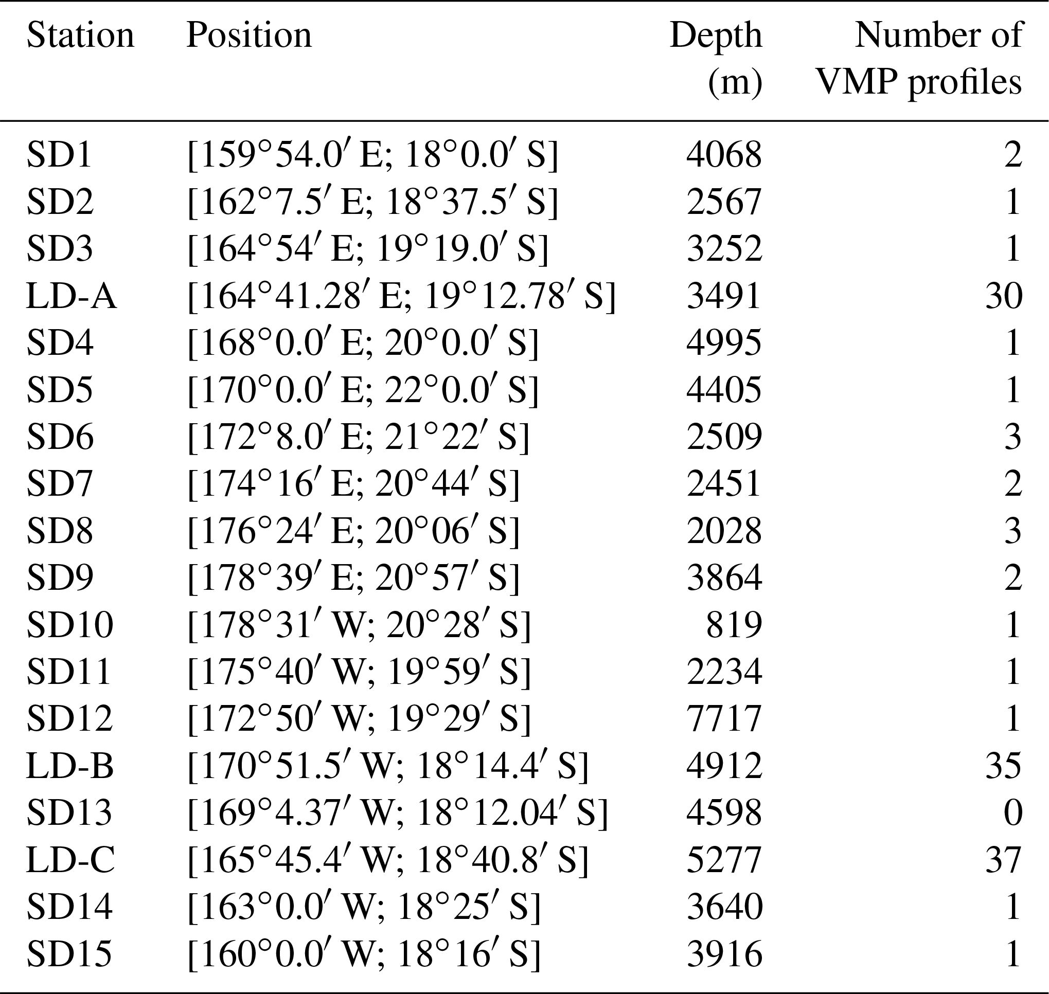
The OUTPACE cruise took place in early 2015 from 18 February to 3 April onboard French oceanographic research vessel l'Atalante (Moutin et al., 2017). A set of 15 short-duration stations (SD) over 24 h as well as 3 long-duration stations (LD) over three inertial periods (the inertial period being ∼36 h) were performed along an almost zonal transect starting from west of New Caledonia and ending near Tahiti (Fig. 1).
2.1 CTD and LADCP
Conductivity–temperature–depth (CTD) measurements were performed on a rosette using a SeaBird SBE 9plus instrument. Data were averaged over 1 m bins to filter out spurious salinity peaks using Sea-Bird electronics software. Simultaneously, currents were measured from a 300 kHz RDI lowered broadband acoustic Doppler current profiler (LADCP). LADCP data were processed using the Visbeck inversion method (Visbeck, 2002) and provided vertical profiles of horizontal currents at 8 m resolution. These measurements were performed at all stations with a typical 3 h time interval between each deployment. In addition the ship was equipped with two SADCPs, RDI Ocean Surveyors with frequencies 150 and 38 kHz yielding processed currents averaged over 2 min time intervals and with vertical bins of 8 and 24 m respectively. Shear was computed using finite differences with current vertical profiles interpolated over a 1 m vertical grid with an estimated noise level of s−1.
2.2 Microstructure measurements with VMP1000
Microstructure measurements were collected using a vertical microstructure profiler, “VMP1000” (Rockland Scientific). This tethered profiler was equipped with microstructure sensors, two shear sensors, and one temperature sensor, as well as with Sea-Bird temperature and conductivity sensors and a high-frequency fluorometer. A total number of 123 profiles were performed with repeated profiles at LD stations (∼ 30 profiles over three inertial periods) and at least one profile at each SD station except at SD13 (see Table 1 for further details). The dissipation rate of turbulent kinetic energy (ϵ) was inferred from centimeter-scale shear measurements. The vertical wavenumber shear spectrum was computed within the inertial range, typically within meter to centimeter scales. The experimental spectrum was next compared to the empirical spectrum, the Nasmyth spectrum (Nasmyth, 1970), which allowed validation of the estimate of ϵ (Ferron et al., 2014). Shear measurements were processed using the routines developed by Rockland Scientific. Specific noise removal procedures were applied with the spikes in the shear data first removed and spectral coherence between the shear sensors and the accelerometers used to remove vibrational contamination. The first 20 m below the surface were not considered to avoid any contamination from the ship wake as well as the 20 m at the end of the profile because of the decreasing vertical velocity there. More generally ϵ values were excluded when the vertical velocity gradient of the VMP was larger than s−1. The averaged ϵ from the two shear probes was taken provided that the ratio between the two estimates was smaller than 2; otherwise, the ϵ value with the smallest depth variation (compared to the neighbouring upper and lower ϵ values) was considered. ϵ was computed over a 1 m depth interval, and then a 8 m moving average was applied to this signal. The estimated noise level is W kg−1 following Ferron et al. (2014).
2.3 Diffusivity estimates
The diapycnal diffusivity, Kz, is commonly inferred from the kinetic energy dissipation rate using the Osborn (1980) relationship:
where Γ is a mixing efficiency defined as the ratio between the buoyancy flux and the dissipation rate, , with w′ and ρ′ the vertical velocity and density fluctuations, and N the buoyancy frequency, inferred from the sorted density profile in order to avoid spurious negative values associated with overturns, , with an 8 m moving average then applied to this signal. Γ was generally set to 0.2 until the recent findings of Shih et al. (2005) and Bouffard and Boegman (2013). These authors found a decrease in Γ for increasing turbulence intensity, I, defined as
where ν is the molecular viscosity, m2 s−1. In terms of timescales, I is the ratio of the square of the Kolmogorov timescale, namely the dissipation timescale of eddies at the Kolmogorov scale (), and the buoyancy timescale (1∕N). Shih et al. (2005) showed in a numerical study that the Osborn relationship overestimated Kz when I>100 and proposed a new parameterization of Kz for this regime. A few years later Bouffard and Boegman (2013) proposed a refined parameterization of Kz including in situ microstructure measurements in lakes as well. They defined different regimes with the following formulations for Kz:
-
m2 s−1 within the diffusive sub-regime, I<1.7 ;
-
within the buoyancy-controlled sub-regime, I within [1.7;8.5];
-
Kz=0.2νI, i.e., the Osborn relationship within the intermediate regime, I within [8.5,400]; and
-
within the energetic regime, I>400.
Note that for the OUTPACE dataset where most I values are smaller than 100, the Kz values inferred from the Bouffard and Boegman parameterization that is applied here do not differ significantly from those inferred from the Osborn relationship.
2.4 Internal forcing: estimates of internal tide generating force and wind power input into inertial motions
The internal tide generation is inferred from the depth integrated generating force following the linear approximation (Baines, 1982) that reads as
where N is inferred from the World Ocean Atlas monthly climatology, ω is the tidal frequency, Q is the barotropic tidal flux, and h is the bottom depth. The barotropic tidal flux is inferred from the global inverse tidal model TPXO (Egbert and Erofeeva, 2002) for two main constituents, the diurnal K1 and the semi-diurnal M2.
The generation of baroclinic near-inertial waves occurs through inertial pumping at the base of the mixed layer (Gill, 1984; Price, 1984). Insight into possible generation of baroclinic near-inertial waves is estimated from the wind work on inertial oscillations following Alford (2003):
where is the square of the wind stress at the inertial frequency, r is the damping of near-inertial motions in the mixed layer as a result of baroclinic near-inertial wave radiation expressed as a function of the inertial frequency r=0.15f, and H is the mixed-layer depth. The wind stress was inferred from numerical simulations over the time period of the cruise (Skamarock et al., 2005) and the mixed-layer depth from the seasonal climatology.
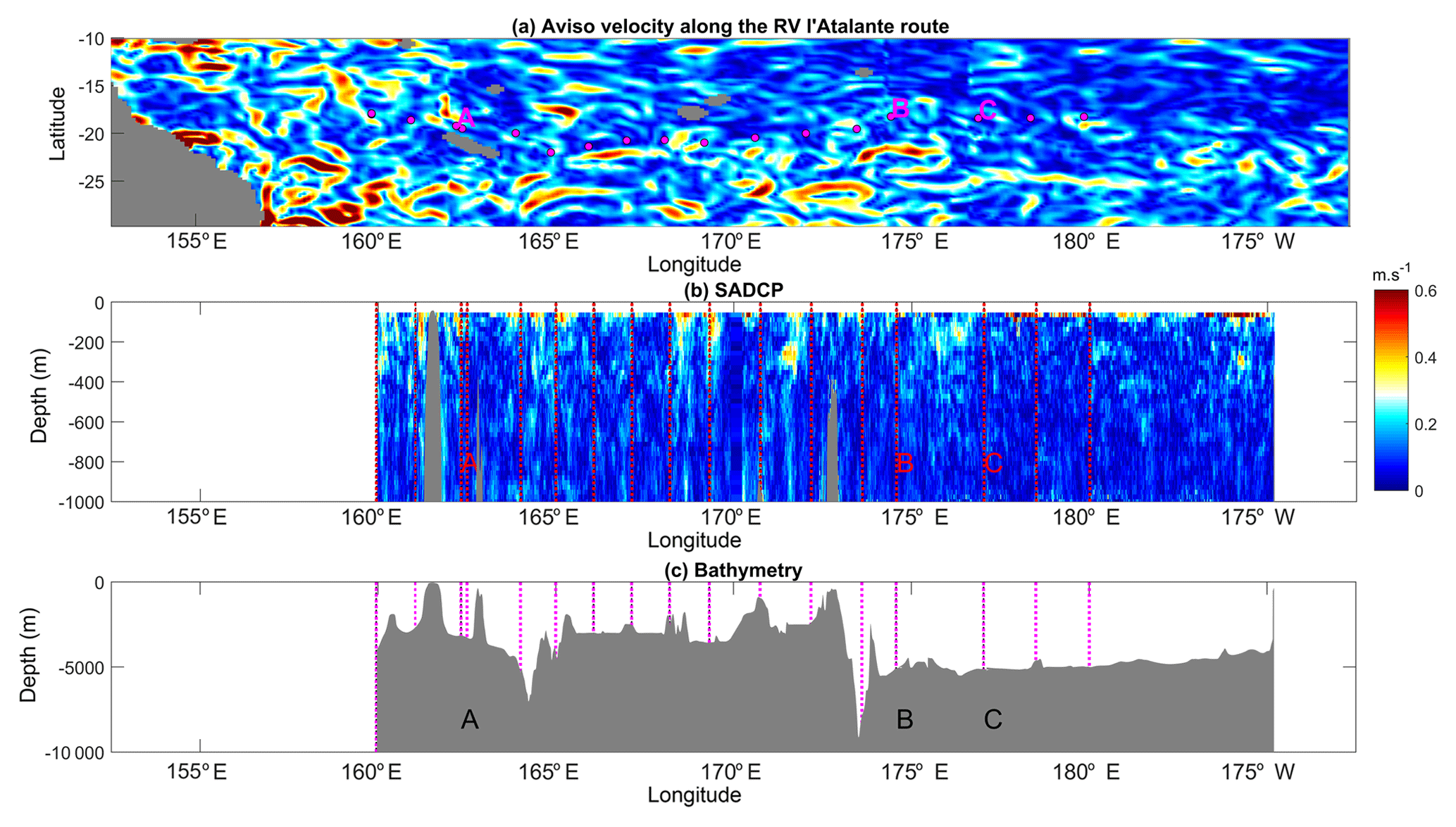
Figure 2Surface geostrophic currents inferred from AVISO altimetric data (a); longitude–depth section of the 38 kHz SADCP velocity modulus (b); bathymetry along the RV l'Atalante route (c); VMP stations are displayed with magenta circles in (a) and with vertical dashed red lines in (b) and magenta lines in (c).
Table 2Statistics in the western and eastern parts: percentage of Ri<1 and mean values and standard deviations of ϵ and Kz within a 100–500 m surface layer.

2.5 Biogeochemical turbulent diffusive fluxes
The vertical components of nitrate and phosphate turbulent diffusive fluxes were computed at all stations, using the diapycnal diffusivity, Kz, inferred from microstructure measurements:
where cNO3 and are the nitrate and phosphate concentrations. Measurements were performed daily at 12 depths in the first 200 m using standard colorimetric procedures Caffin et al. (2018). The quantification limits were 50 µmol m−3. At LD stations where six profiles were obtained, the quantification limit for the mean concentration dropped to 20 µmol m−3 (i.e., ). Concentration values below the threshold for quantification were set to NaN. Vertical concentration profiles were interpolated over a 1 m vertical grid and a 10 m moving average was next applied. The top of the nitracline was defined as the depth where nitrate concentration is zero based on an extrapolation from the last detectable concentration (>50 µmol m−3) assuming a constant vertical gradient above this depth Moutin et al. (2018). It is only at long-duration stations that the top of the nitracline was defined in isopycnal coordinates: this allows us to get rid of a varying depth of the nitracline because of vertical displacements of isopycnals induced by internal waves Caffin et al. (2018). The minimum turbulent diffusive flux was estimated from the threshold concentration with the molecular Kz value ( m2 s−1): 0.4 at SD stations and 0.17 at LD stations where the mean concentration profile was taken to compute the flux. A reference profile was also defined in order to compare the nitrate diffusive flux variations along the OUTPACE within a 100 m layer below the top of the nitracline. To do so vertical profiles of concentration were first shifted vertically so that the reference depth matched with the top of the nitracline and the mean vertical profile within the nitracline was inferred from this set of re-scaled concentration profiles. Kz profiles were also rescaled onto this vertical grid and a mean Kz profile inferred. The relative contributions of the variations in Kz and that of with respect to the total variations of the flux were also inferred.
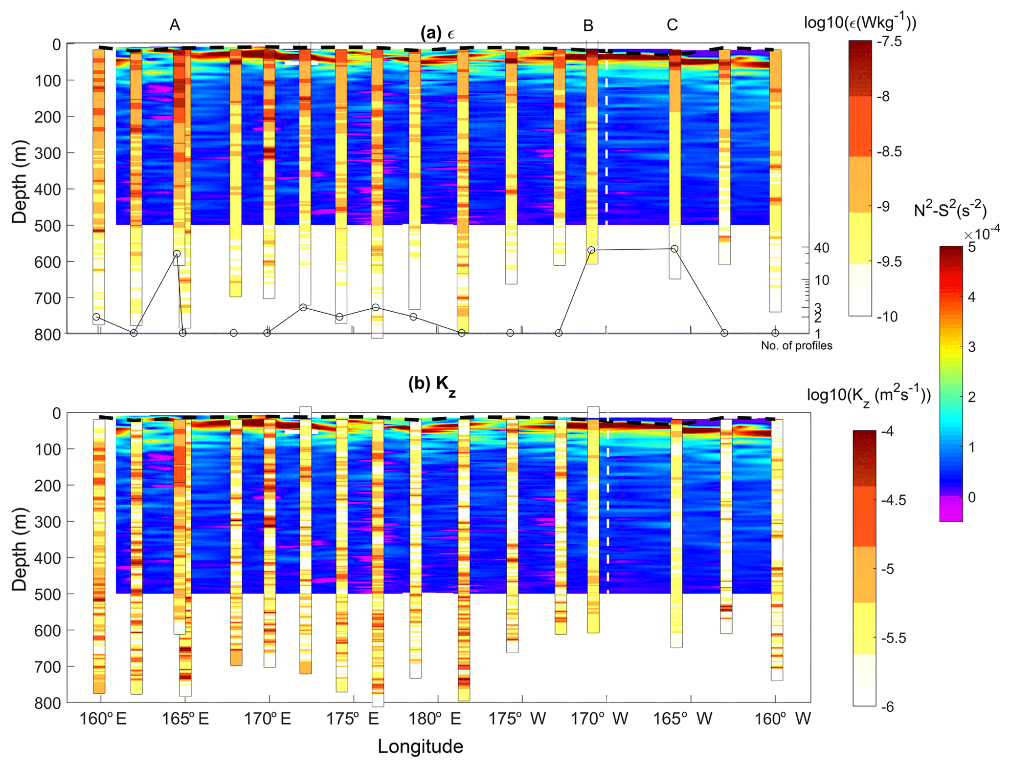
Figure 3Log values of the dissipation rate of turbulent kinetic energy (W kg−1) (a) and vertical diffusion coefficient (m2 s−1) (b) with N2−S2 in background color scale. The number of profiles at each station is displayed with black circles and profiles have been time-averaged at each station for better visualization. The mixed-layer depth is plotted (black dashed curve) as well as the limit between the two regions (dashed white line).
3.1 Overview
An overview of the spatial pattern of turbulence is given with depth-averaged values of ϵ and Kz below 100 m depth at each station (Fig. 1). Depth-averaged dissipation rates, 〈ϵ〉, vary within an order of magnitude within W kg−1. The highest values are observed west of 170∘ W, in the shallower part, while the lowest values are observed east of 170∘ W, in the deeper part. The same contrast is retrieved on 〈Kz〉 with values ranging within m2 s−1. The western part of our study area which shows the highest turbulence level is also the region where the most intense velocities are observed, as illustrated with altimetry-derived currents produced by AVISO along the RV l'Atalante cruise path (Fig. 2a). The vertical section of the total velocity modulus inferred from the SADCP data shows that this contrast is also observed at depth with slightly larger velocities in the western part of our study area (Fig. 2b). There the bathymetry ranges typically from 4000 m up to a few hundred meters locally with significant topographic slopes, which is consistent with the higher velocity signal; by comparison, in the east the bathymetry is almost flat, with ∼5000 m depth. More insights into turbulence are given with vertical sections of ϵ and Kz in Fig. 3a and b. The range of ϵ values covers 3 orders of magnitude, W kg−1 below the mixed layer (magenta curve in Fig. 3a) down to 500 m depth. ϵ presents a typical patchy pattern with spots of intense turbulence with values up to W kg−1 down to 500 m. These events are localized over a 10 m vertical scale except at LD-A around 165∘ E longitude where a 200 m layer of enhanced ϵ is observed. Most of these events are observed in the west, west of 170∘ W, and the few vertically localized large ϵ observed east of 170∘ W are no deeper than 200 m depth (Fig. 3a). Statistics of ϵ within a 100–500 m depth interval are given for each region in Table 2. The contrast between the mean 100–500 m depth-averaged ϵ in each of the two regions is a factor of 3 (Table 2). The contrast is larger for the standard deviation, a factor of 10, which points to the larger intermittency of turbulent events west of 170∘ W. The Kz pattern presents a similar contrast between the western and eastern parts with mean 100–500 m depth-averaged Kz between the two regions differing by a factor of 2 (Table 2). More importantly, the standard deviation of Kz is by far larger west of 170∘ W, by a factor of 15 (Table 2).
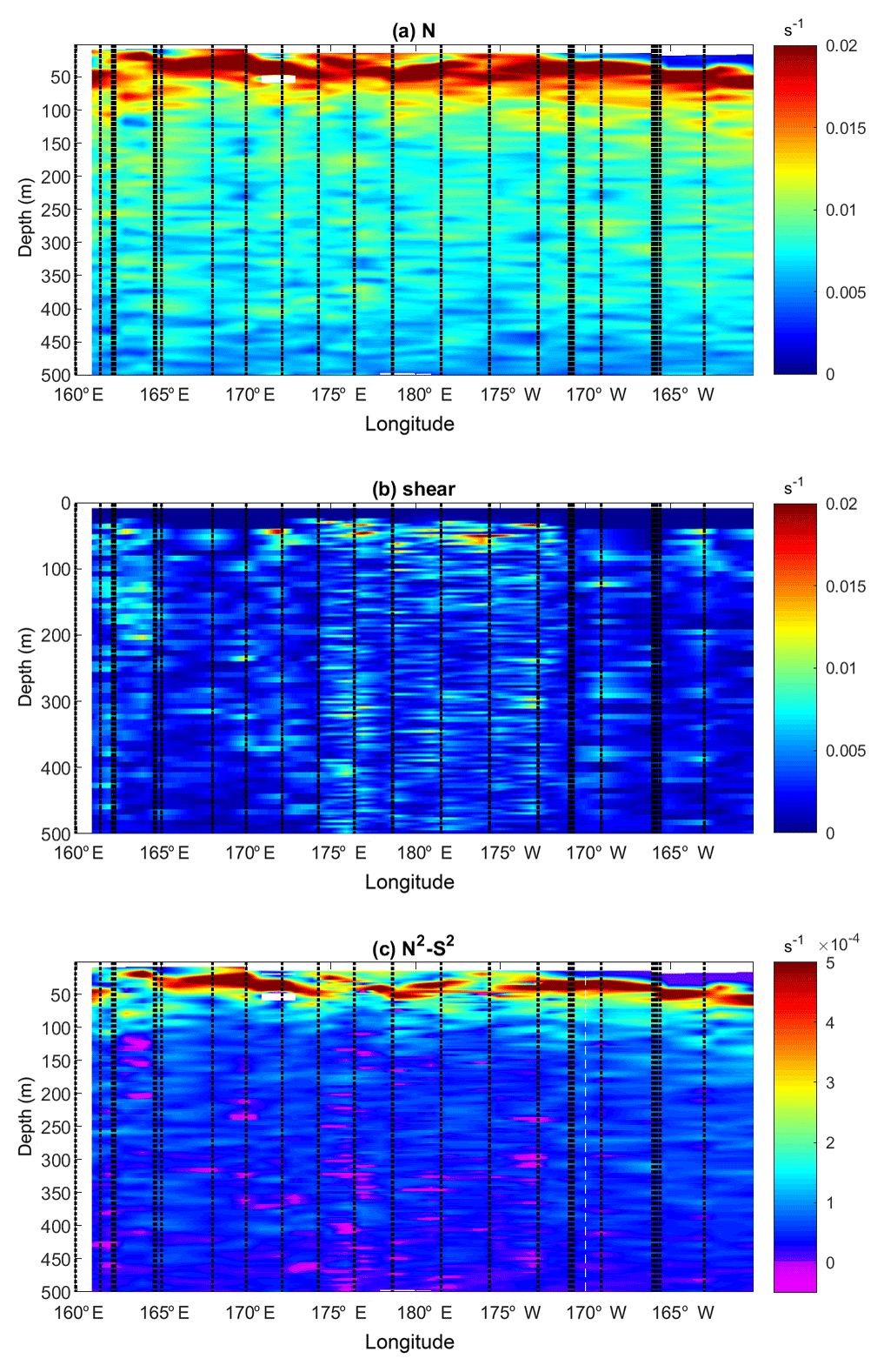
Figure 4Buoyancy frequency, N (a), shear, S (b), and N2−S2 (c) as a function of longitude and depth. The locations of the CTD and LADCP profiles are displayed with black dashed lines. S is inferred from LADCP data and N was vertically averaged over 8 m length vertical intervals for consistency with the 8 m bin of the LADCP data.
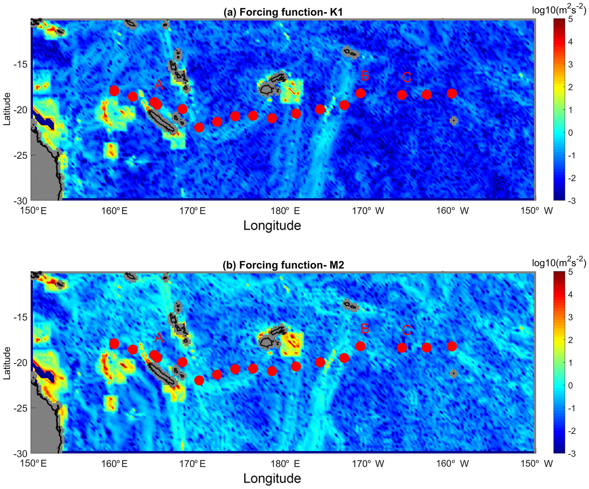
Figure 5(a) Depth-integrated generation force for the K1 tidal constituent (log10(m2 s−2)); (b) same as in (a) but for the M2 tidal constituent. The stations are shown with a red circle and the LD stations are indicated.
3.2 Shear instability
To gain further insights into the origin of this contrast in turbulence, the possible occurrence of shear instability is addressed with buoyancy frequency, N, shear, S, and N2−S2 sections displayed in Fig. 4. The stratification is strong in the first 100 m, with a pycnocline that is generally well marked except westward of 165∘ E and around 172∘ W longitudes and a less stratified surface layer above 50 m east of 170∘ W. The shear is significantly higher west of 170∘ W, with high values over the 500 m depth layer of the measurements in the west except for a 165–170∘ E region (Fig. 4a and b). The likeliness of shear instability was estimated from N2−S2, displayed in Fig. 4c. The upper 100 m surface layer is the most stable, with the highest N2−S2 values as a result of both strong stratification and low shear. Shear instability is more likely to occur west of 170∘ W below the 100 m surface layer of strong stratification and where the shear is large: the percentage of data points that verifies the criterion for shear instability is 10 times larger west of 170∘ W than east of 170∘ W (Table 2). The fact that most of the subcritical Ri, , are observed west of 170∘ W is consistent with the enhanced dissipation observed there (Fig. 3 and 4c).
3.3 Tidal and atmospheric forcings for the internal wave field
The possible impact of internal waves was estimated indirectly through the two main energy sources of these waves, namely tidal forcing and wind power input (Figs. 5 and 6).
The depth-integrated tidal generation force is displayed in Fig. 5 for the K1 and M2 constituents. There is a strong similarity between the two constituents with a generation that is favoured in the western part which is shallower and with stronger topographic gradients than the eastern part of our study area. The westernmost region is characterized by numerous spots of generation with a depth-integrated generation force of 103 m2 s−2, while eastward of 170∘ E longitude there is only one main generation site around 180∘ E longitude (Fig. 5a). This spatial distribution of the internal tide forcing might suggest a similar contrast in the internal-tide-induced dissipation since the high modes responsible for turbulence are expected to dissipate within a few tens of kilometers of the generation site (St Laurent et al., 2002).
Maps of wind power input on inertial motions, also referred to as inertial flux, were computed using the spectral method described by Alford (2003). The wind stress data were inferred from WRF numerical simulations (Klemp et al., 2007; Skamarock et al., 2005) and the seasonal climatology was used for the mixed-layer depth. The power input into inertial motions gives insights into the generation of baroclinic near-inertial waves (niw) at the base of the mixed layer through inertial pumping (Gill, 1984). The maps reveal a strong longitudinal contrast in inertial flux until mid-March (Fig. 6a–e). The strongest wind power input was observed in the western part of our study area. This is consistent with the climatology of storms and cyclones in the area that are typically formed in the south-western tropical Pacific Diamond et al. (2013). At the beginning of the cruise the largest power input was localized south-west of the cruise stations (Fig. 6a). Later a major event was observed (Fig. 6d) during the passage of a tropical cyclone over the area while RV l'Atalante was sampling to the east. Eventually by the end of the cruise the inertial flux was small over the OUTPACE region, with one spot of weak inertial flux observed in the east (Fig. 6f–g). These maps suggest that energetic niw are likely to be generated in the western part of our study area prior to the cruise and until mid-March (Fig. 6a–b). The first event of large inertial flux prior to the cruise may be particularly insightful since it is likely to lead to the generation of equatorward propagation niw within the OUTPACE sampling area, a scenario which is consistent with large ϵ values there (Fig. 1).
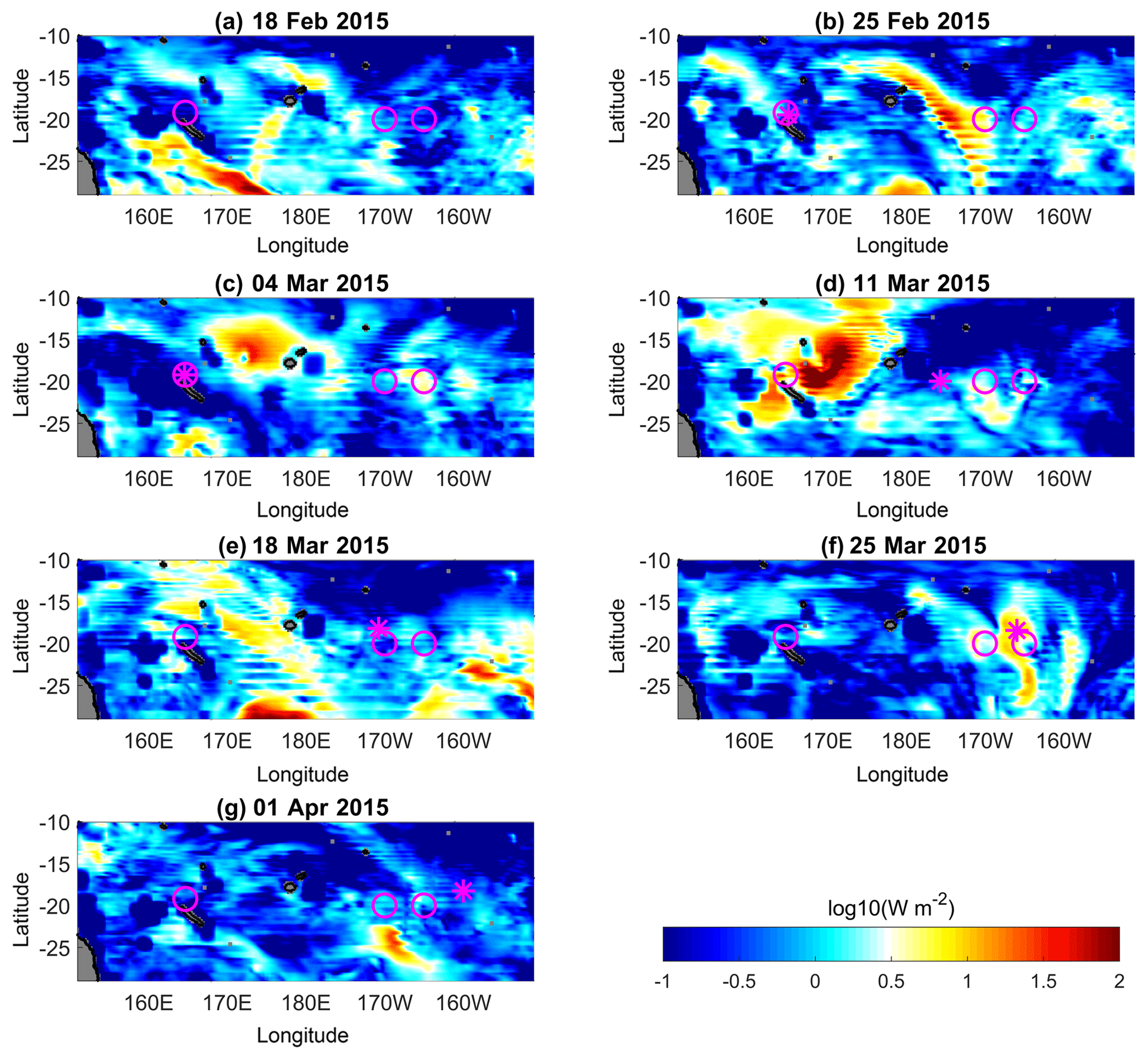
Figure 6Maps of inertial energy flux (log10(W m−2)) every 7 days during the cruise. Long-duration stations are shown with magenta circles, and LD-A was held during (b) and (c), LD-B during (e), and LD-C during (f). The ship position is displayed with a magenta star.
Three long-duration stations were sampled each over three inertial periods, LD-A in the western part of the transect and LD-B and LD-C in the eastern part of the transect (see Table 1 and Fig. 1). Turbulence at LD-A is by far the largest down to 500 m depth, with contrasted mean ϵ and Kz between LD-A on the one hand and LD-B and LD-C on the other hand (Fig. 7a and b) by factors of 7 and 5 for the averaged, within [100 m, 500 m], ϵ and Kz respectively (Table 3). Possible occurrence of shear instability is examined by comparing mean profiles of shear square, S2, and N2 (Fig. 7c). While the mean stratification is fairly close, at the three stations the shear square is larger at LD-A compared to LD-B and LD-C within a factor of 10 within [50 m, 250 m] (Fig. 7c). Furthermore, within [100 m, 200 m] S2 is larger than N2 at LD-A, pointing to possible shear instability. This depth range coincides with local ϵ maxima, thus reinforcing the shear instability hypothesis.
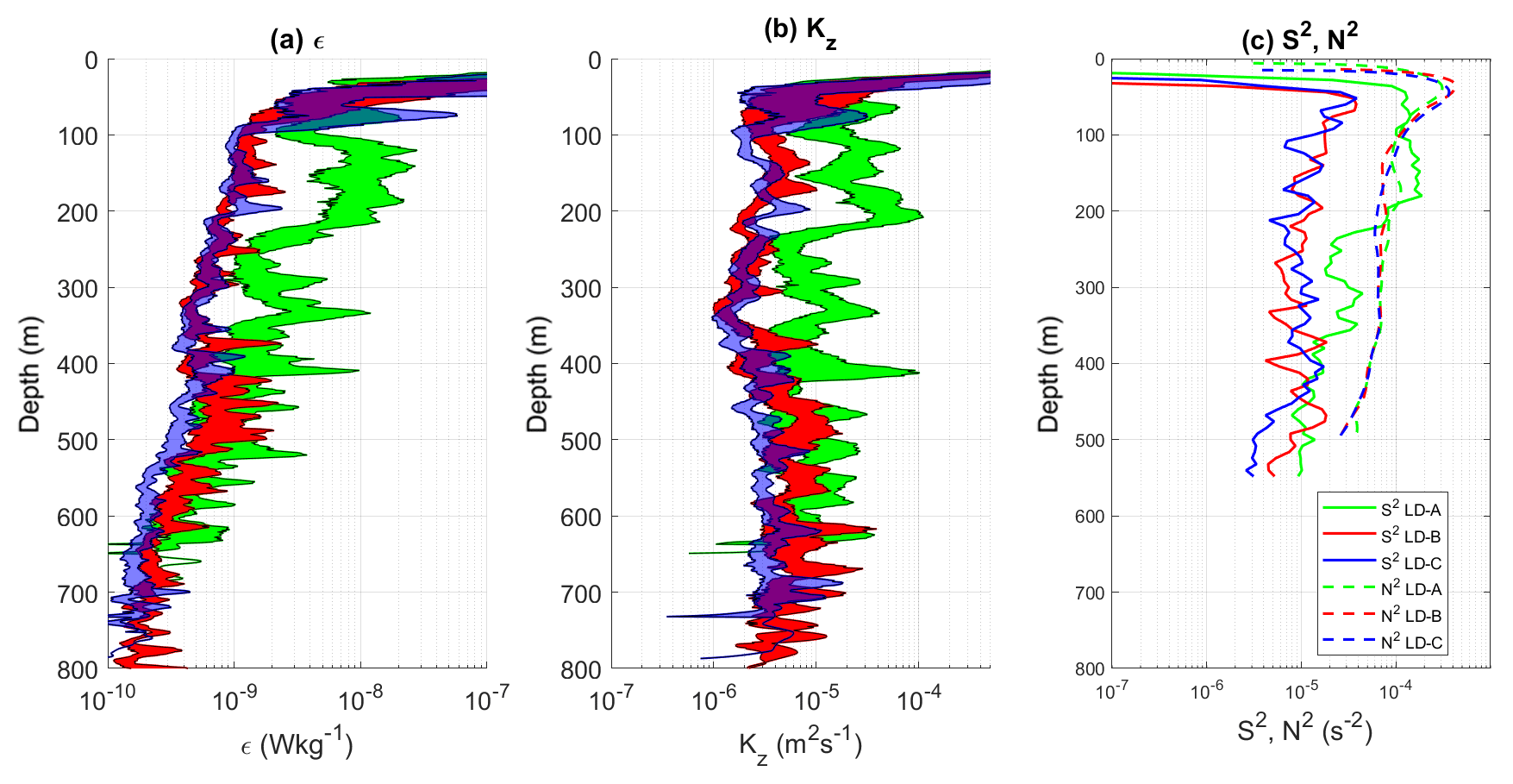
Figure 7Mean profiles at long-duration stations: ϵ in (a), Kz in (b), and S2 and N2 in (c). Kz was computed using N from the VMP measurements, while the profiles in (c) were inferred from the rosette-mounted CTD and LADCP instruments. The 95 % confidence interval for ϵ and Kz is displayed with a shading surface in (a) and (b).
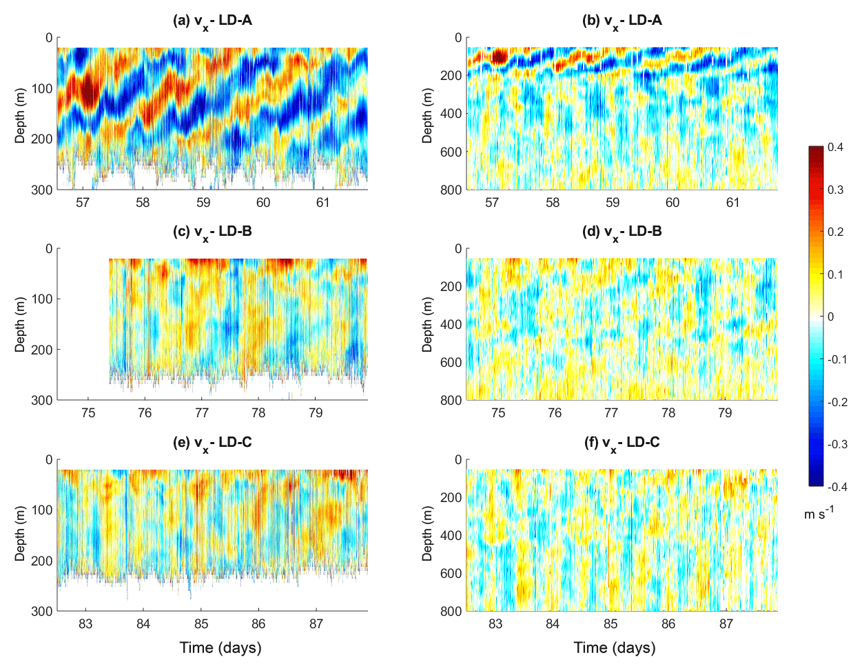
Figure 8Zonal velocity (m s−1) as a function of time and depth at the long-duration stations; each row from 1 to 3 corresponds to LD-A, LD-B, and LD-C respectively. In the first column ship ADCP data from the 150 kHz instrument down to 300 m are displayed and in the second column those from the 38 kHz instrument down to 800 m. Note that in (b) the 150 kHz SADCP functioned only a few hours after the beginning of the station sampling.
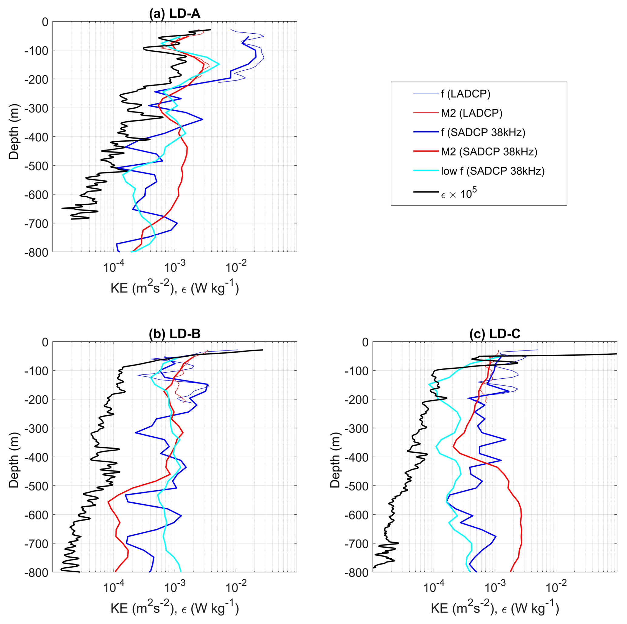
Figure 9Time-mean profiles of the kinetic energy of the subinertial flow, the inertial and semi-diurnal frequencies, and ϵ at LD-A (a), LD-B (b), and LD-C (c). The kinetic energy was derived from the 38 kHz SADCP data but also from the 150 kHz SADCP data for the inertial and semi-diurnal kinetic energies (thin blue and red curves).
We next focused on the characterization of the internal wave field that may reinforce the vertical shear and contribute to the onset of turbulence. Current magnitude at LD-A is the largest (Fig. 8a and b), of the order of 0.4 m s−1. Detailed insights from the 150 kHz SADCP reveal a wavy pattern with two frequencies clearly identified (Fig. 8a): strong upward-propagating bands close to the inertial period, of about 1.5 days, and the semi-diurnal period, which manifests itself through semi-diurnal heaving of upward-propagation niw bands. The former is observed over the first 200 m only, while the latter is observed down to ∼800 m depth (Fig. 8a and b). The weaker currents at LD-B and LD-C are comparable with a maximum amplitude of 0.2 m s−1 (Fig. 8c–f). Periodic motions are also evidenced with inertial oscillations in the first few meters (Fig. 8c) and a combination of near-inertial and tidal periods at depth. Noticeably, an upward phase propagation of niw can be inferred at LD-B from the 38 kHz SADCP data (Fig. 8d). At LD-C the semi-diurnal tidal signal dominates (Fig. 8f). The dominance of niw at LD-A is consistent with the highest wind power input inertial motions at LD-A (Fig. 6a) compared to LD-B and LD-C (Fig. 6e). Instead the contrast observed between the semi-diurnal depth-integrated generating force at LD-A compared to that at LD-B and LD-C (Fig. 5b) is not evidenced on the semi-diurnal currents (Fig. 8). This is well evidenced below ∼300 m depth where the semi-diurnal tidal signal dominates at all stations (Fig. 8b, d, and f). This difference might result from localized generation areas of small scales that are not predicted by the estimate performed with low-resolution fields (tidal model and bathymetry) or from low modes with long-range propagation.
Table 3Statistics at the long-duration stations: percentage of (i.e., Ri<1), median values of ϵ, Kz, mean value of kinetic energy for the sub-inertial frequencies, inertial frequency and semi-diurnal M2 tidal constituent, and the same for shear variance. The average is performed over a 100–500 m surface layer (first three lines) as well as over a 50–250 m layer to highlight the impact of the niw at LD-A.
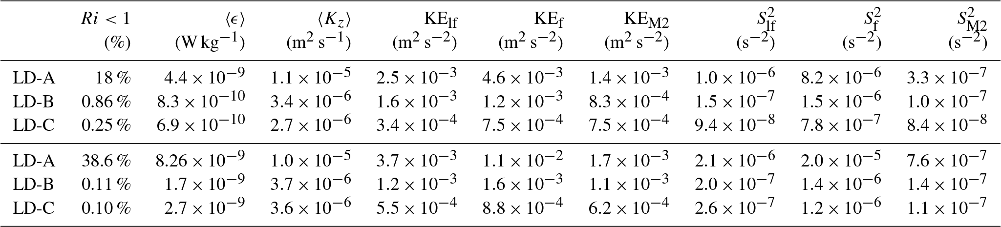
Table 4Statistics in the western and eastern parts: mean values of the NO3 and PO4 turbulent diffusive fluxes in the photic layer. The standard deviation is given within the brackets.
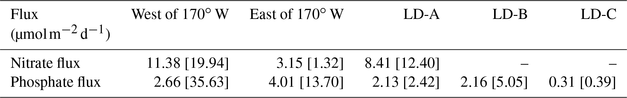
Figure 9 summarizes the main characteristics of the three long-duration stations, with vertical profiles of time-averaged ϵ and kinetic energy for the sub-inertial flow, the inertial frequency band, and the semi-diurnal tidal constituent, M2. Kinetic energies were inferred from the frequency spectra computed over three inertial periods. Depth-averaged values of ϵ, Kz as well as kinetic energy and shear within the different frequency bands are also given in Table 3. The average was computed over two depth intervals: the first one is 100–500 m, consistent with that chosen in Table 2, while the second one is 50–250 m, corresponding to the depth interval of maximum niw energy at LD-A. The enhanced ϵ at LD-A is coincident with an energetic niw (Fig. 9a). The contrast with LD-B and LD-C is striking within the depth interval 50–250 m with an averaged ϵ within 50–250 m about 8 times larger than at LD-B and a near-inertial kinetic energy that differs by almost an order of magnitude (Table 3). The significant decrease in ϵ, coincident with a sharp shutdown of the near-inertial baroclinic signal around 250 m, shows the main effect of niw on dissipation. This transition is associated with a strong variation in the subinertial flow that suggests a wave mean flow interaction Soares et al. (2015). LD-B and LD-C present strong similarities in ϵ and niw and M2 kinetic energies with 100–500 m depth-averaged values that are close (Table 3). The local maxima in near-inertial kinetic energy may evidence niw beams around 150, 450, and 650 m at LD-B and 200, 350, 400, and 650 m at LD-C (Fig. 9b and c). The semi-diurnal kinetic energy presents an interesting contrast between LD-B and LD-C: while it is larger at LD-B in the first 500 m and smaller below, the opposite is observed at LD-C with maximum semi-diurnal energy below 500 m depth, also suggesting a beam structure. The subinertial flow is weakest at LD-C (Fig. 9c) by a factor of 2 compared to LD-B and by a factor of 8 compared to LD-A for the 100–500 m depth-averaged value of the kinetic energy. Moreover, the depth-averaged low-frequency shear is below the noise level at LD-B and LD-C (Table 3), both features suggesting a weak influence on internal wave propagation. The subinertial flow is by far the largest at LD-A down to ∼250 m (Fig. 9a). The contrast in turbulence between the three stations is mostly confined in the upper few hundred meters as a result of an energetic niw and its interaction with the strongly sheared subinertial flow (Table 3). Deeper, variations in ϵ and kinetic energies are much weaker and of the same order of magnitude at the three stations (Fig. 9).
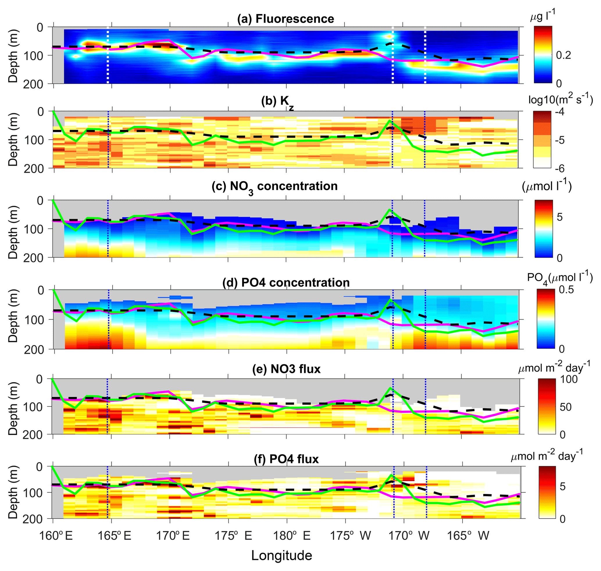
Figure 10Longitude–depth sections of chlorophyll concentration (a), Kz (b), nitrate concentration (c), phosphate concentration (d), nitrate turbulent diffusive flux (e), and phosphate turbulent diffusive flux (f). The top of the nitracline is shown with a magenta line, the depth of maximum chlorophyll concentration with a green line, and the euphotic zone depth with a dashed black line. The locations of the LD stations are shown with a vertical dashed line. The scales of the color bar of the nitrate and phosphate concentration and turbulent diffusive flux are set to allow a direct comparison of concentrations and fluxes against nutrient requirements for phytoplankton (Redfield proportion: ).
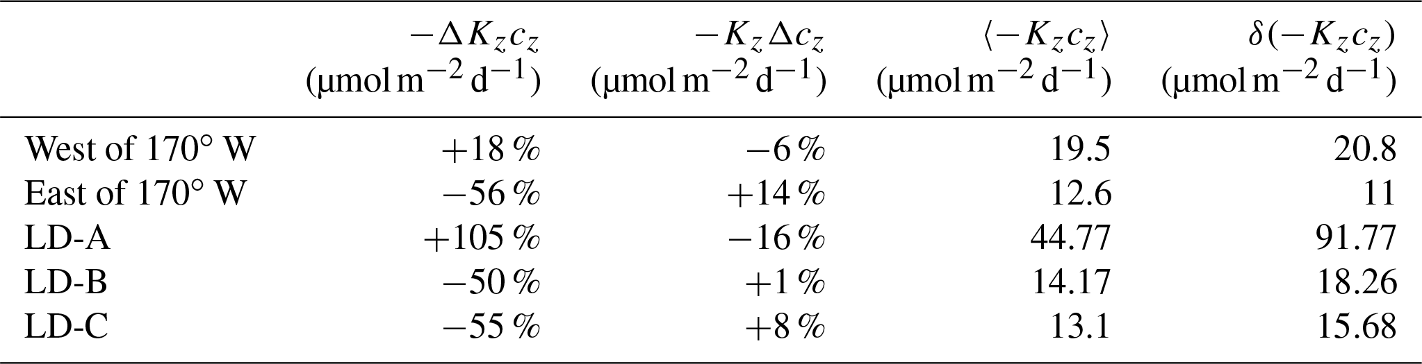
Table 5Relative contributions to the flux variations of Kz and cz depth-averaged over a 100 m vertical layer defined from the top of the nitracline, west of 170∘ W and east of 170∘ W and at long-duration stations. The mean value and standard deviation are also given.
5.1 Overview of the OUTPACE section
The distribution of chlorophyll concentrations along the OUTPACE transect is typical of a transition from an oligotrophic area in the MA toward an ultra-oligotrophic area in the SPSG (Moutin et al., 2017) with a deepening of the deep chlorophyll maximum, DCM, from ∼60 to ∼160 m and an increase in the euphotic zone depth (Fig. 10a). There is one noticeable exception to this trend with a near-surface chlorophyll concentration maximum at ∼35 m depth, at LD-B. de Verneil et al. (2017), who focused on the characterization of this anomalous phytoplankton bloom event, explained its occurrence by the main impact of mesoscale advection and an island effect. The deepening of the DCM results from that of the nitracline and from the NO3 depletion in the first 200 m, an evolution consistent with the increasing oligotrophy to the east (Fig. 10a and c). Moreover, east of 172∘ W the nitracline is most often deeper than the base of the euphotic layer, which reinforces the oligotrophy. The turbulent diffusive nitrate flux displays the same longitudinal trend (Fig. 10c) with a depth-averaged value in the photic layer that differs by almost a factor of 4 west of 170∘ W and east of 170∘ W (Table 4). The standard deviation is also by far larger in the west, by a factor of 15. Whether these flux variations are driven by Kz variations or cz variations was examined within a 100 m depth interval below the nitracline all along the section. These large variations of the turbulent diffusive nitrate flux at small scales (Fig. 10c) mostly result from Kz variations with a weaker contribution of variations in the vertical gradient of nitrate concentration with a typical ratio of 3 between the two (Table 5). The latter contribution tends to weaken slightly the eastward decrease in the flux due to decreasing Kz. The variation of the nitrate diffusive flux was also examined at LD stations only in order to focus on the impact of the temporal intermittency of turbulent events at each LD station where a large number of VMP profiles were collected. The flux variation resulting from Kz variations, −ΔKzcz, and those resulting from cz variations, −KzΔcz, were compared to the averaged flux over the three LD stations. The −ΔKzcz always dominates and is by far the largest at LD-A, with a relative value of 105 % compared with the −50 % and −55 % relative values at LD-B and LD-C (Table 5). This shows the major impact of the turbulence intermittency induced by the niw event at LD-A.
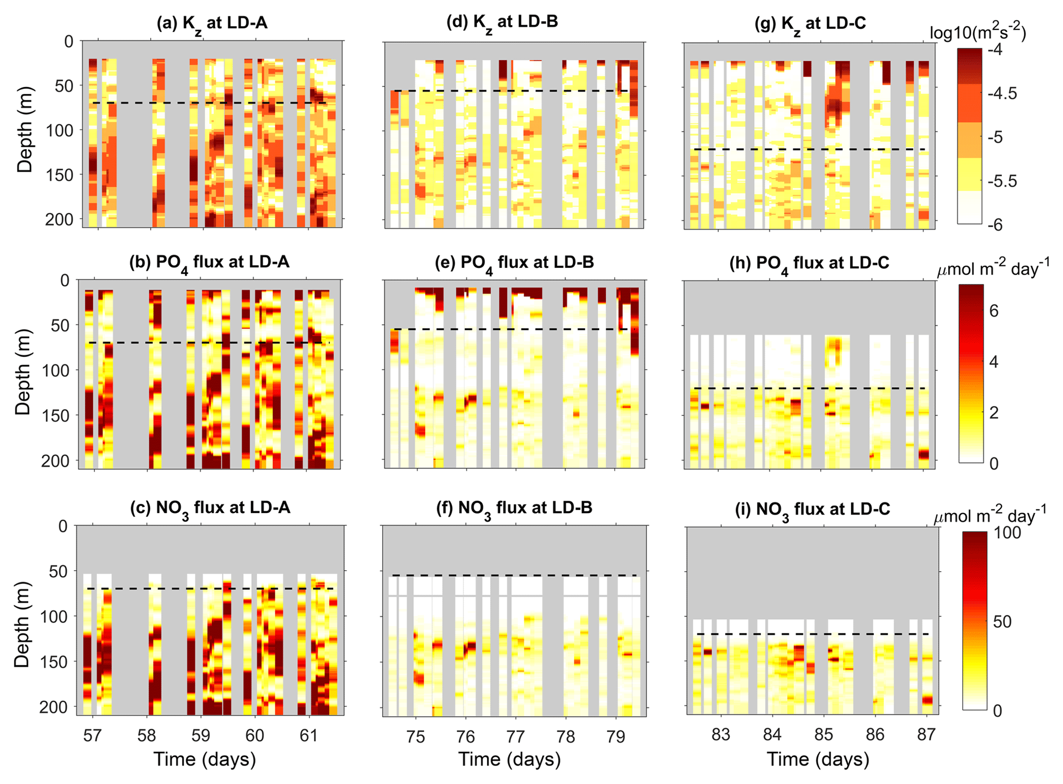
Figure 11Time–depth sections of Kz (a, d, g), phosphate turbulent diffusive flux (b, e, h), and nitrate turbulent diffusive flux (c, f, i). The scales of the color bar of the nitrate and phosphate diffusive flux are set to match with the typical Redfield ratio in the area (). The mean euphotic zone depth is displayed with a black dashed line. The top of the nitracline is defined by the isopycnal and falls at depths of ∼83.5 m at LD-A, ∼111.2 m at LD-B, and ∼134.6 m at LD-C.
Phosphate turbulent diffusive flux is on average smaller than the nitrate turbulent diffusive flux, but its relative impact may be rescaled by a factor of 16 : 1 corresponding to the Redfield N : P ratio. Hence, for visual comparison between the two fluxes, the scale for the phosphate turbulent diffusive fluxes differs from that of the nitrate turbulent diffusive flux within the Redfield ratio in Fig. 10 and subsequently. The phosphate turbulent diffusive flux displays a similar longitudinal gradient in the first 200 m but presents an opposite trend in the photic layer, with a depth-averaged value higher by a factor of 1.5 east of 170∘ W (Table 5). The concentration of phosphate is not as strongly limiting as that of nitrate in the photic layer with significant turbulent diffusive flux, in a few spots, especially around 170 and 190 longitudes (Fig. 10d). Consistently the same trend is obtained for the phosphate concentration in the photic layer, with an eastward increase in the photic layer as opposed to the nitrate concentration that tends to zero at the eastern stations (Fig. 10c and d). The absolute value of the photic layer depth-averaged value of the flux, east of 170∘ W, is 4.01 . Considering a N : P Redfield ratio of 16, the phosphate turbulent diffusive flux is significant compared to the 3.15 value for the nitrate turbulent diffusive flux (Fig. 10e and f, Table 4). This striking difference in phosphate and nitrate turbulent diffusive fluxes within the photic layer may play an important role in the development of micro-organisms as discussed later.
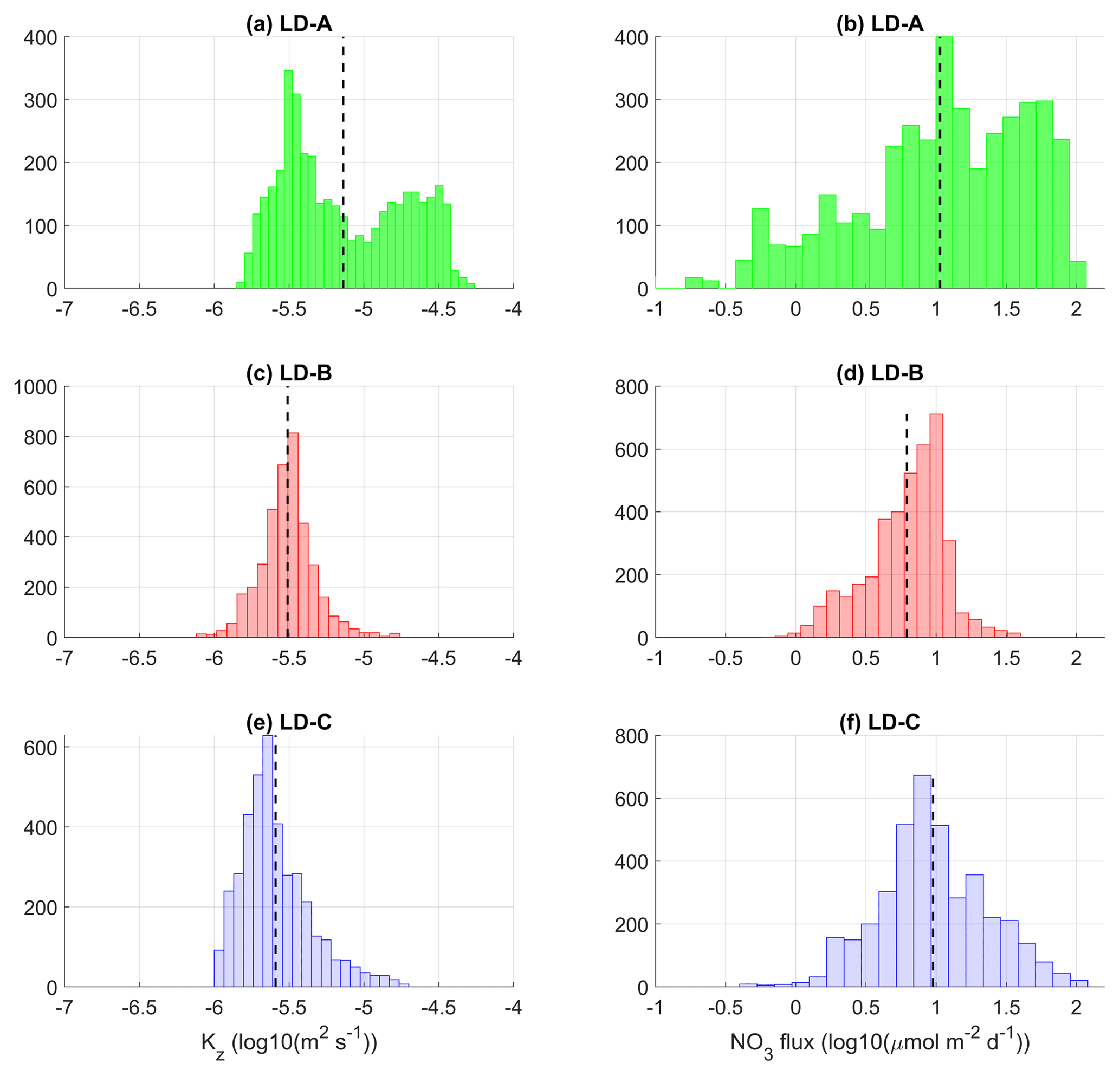
Figure 12Histograms of Kz (a, c, e) and nitrate turbulent diffusive flux (b, d, f) at long-duration stations LD-A, LD-B, and LD-C around the top of the nitracline. The top of the nitracline is defined by the isopycnal, , with density values taken from Caffin et al. (2018), Table 4. A density interval of the upper bound equal to kg m−3, of a typical vertical extension equal to 3–4 m, was chosen for the statistics. The mean value is shown in each subpanel with a dashed line.
5.2 Focus on LD stations
Turbulent diffusive fluxes of nitrate and phosphate were further analysed at long-duration stations (Fig. 11). The time–depth evolution of Kz underlines the very large values encountered at the most turbulent station, LD-A, in contrast with values at LD-B and LD-C that show the occurrence of a few spots of intense mixing in a more quiescent background with m2 s−1 (Fig. 11a, d, and g). The largest nitrate turbulent diffusive fluxes occur at LD-A (Fig. 11b), while the smallest values are observed at LD-B and LD-C (Fig. 11f and i). The averaged values in the photic layer show that it is only at LD-A that there is a small input of nitrate through diffusion with an average flux of 8.41 (Table 4).
In contrast, phosphate turbulent diffusive fluxes are significant well above the euphotic zone depth at all LD stations (Fig. 11b, e, and h), which may have an impact on primary production, whereas the nitrate input by turbulent diffusion is negligible (explanation below). Depth-averaged values in the photic layer are even comparatively larger than that of the nitrate turbulent diffusive fluxes at LD-A if one applies the Redfield ratio (Table 4). Various spots of large phosphate turbulent diffusive fluxes are also evidenced in the first ∼ 20–80 m that can be correlated with events of intense turbulence (Fig. 11b, e, and d). At LD-C the only event of significant phosphate turbulent diffusive flux results from a strong turbulent event (Fig. 11h).
5.2.1 Nitrate input at the top of the nitracline
The input of nitrate through turbulent diffusion was first examined at the top of the nitracline, within a ∼4 m thickness layer, with histograms of the nitrate turbulent diffusive flux (Fig. 12). There is a strong contrast between LD-A and the eastern stations in the shape of the histograms: an atypical shape of the histogram is obtained at LD-A with a large standard deviation, while the distribution of the nitrate turbulent diffusive flux is fairly similar at LD-B and LD-C with one main peak (Fig. 12d and f). The atypical shape obtained at LD-A results from the large intermittency of Kz as illustrated in Fig. 12a. The distribution of Kz values covers 2 orders of magnitude and presents a bimodal distribution. The moderate Kz values are associated with the “background state”, while the large values are associated with intense turbulent events related to the near-inertial baroclinic wave (e.g., Fig. 8a). The mean value of the nitrate turbulent diffusive flux within a ∼4 m layer starting from the top of the nitracline is smaller at LD-B compared to LD-A and LD-C: 24.1 and 18.9 at LD-A and LD-C compared with the mean value of 6.0 at LD-B. This contrast may appear surprising, with a comparable mean value at LD-A and LD-C, but this results from the occurrence of a few turbulent events at LD-C where the nitracline is deepest. Nevertheless, the main point regarding the impact of the turbulent input of nitrate at the top of the nitracline on new primary production is whether or not the top of the nitracline falls within the photic layer. This point is addressed in the following with histograms in the photic layer.
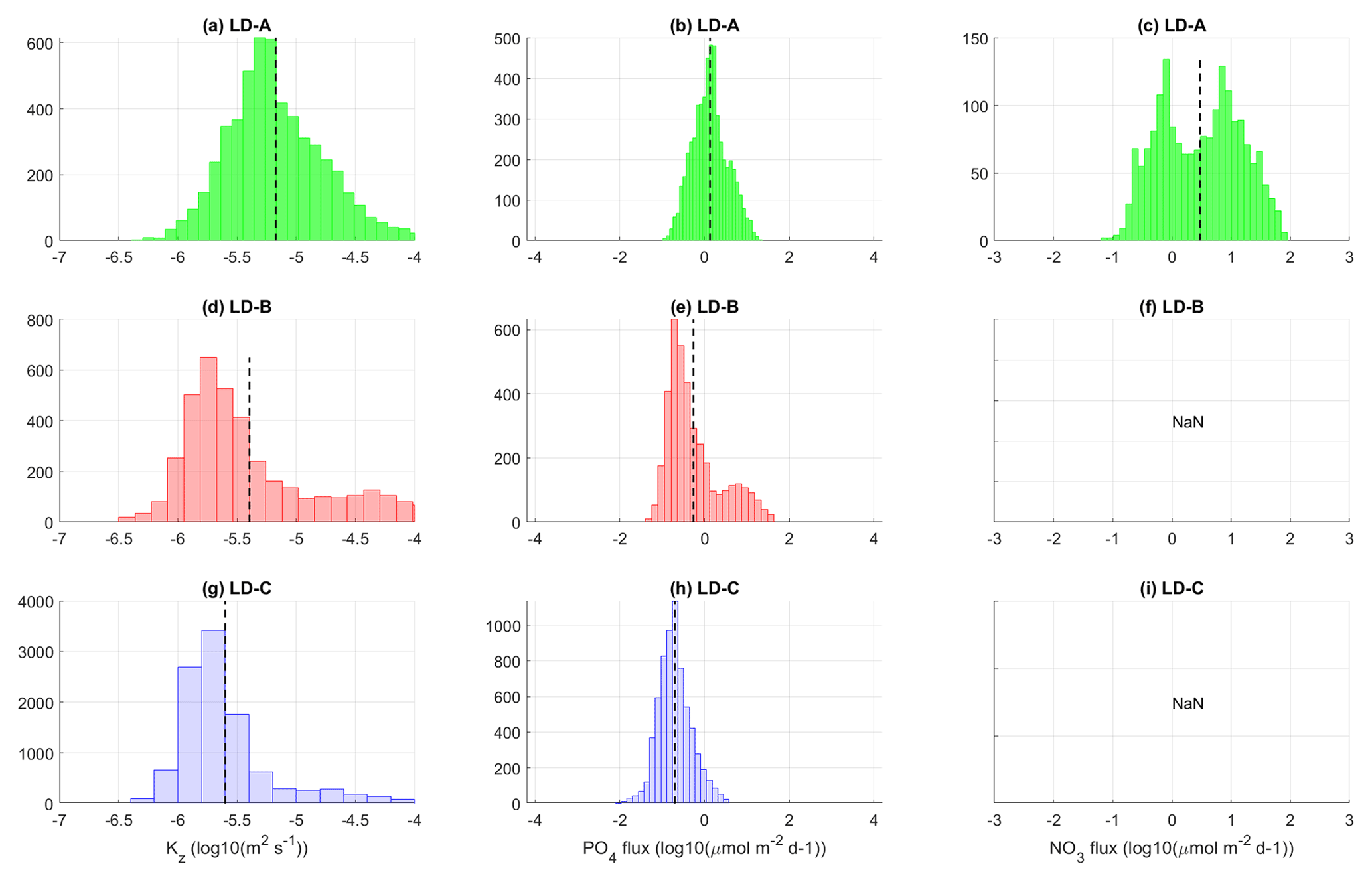
Figure 13Histograms of Kz (a, d, g), phosphate (b, e, h), and nitrate (c, f, i) turbulent diffusive fluxes at long-duration stations LD-A, LD-B, and LD-C within the photic layer (down to 70, 55, and 120 m respectively). At LD-B and LD-C the nitrate turbulent diffusive flux is below the noise level within the considered depth interval (f, i). The mean value is displayed with a dashed black line.
5.2.2 New primary production sustained by phosphate turbulent diffusive fluxes at the western stations?
Figure 13 summarizes the contrast between long-duration stations in the photic layer with histograms of Kz, phosphate, and nitrate turbulent diffusive fluxes. The euphotic zone depth (EZD) was immediately determined on board from the photosynthetically available radiation (PAR) at depth compared to the sea surface PAR(0+), and used to determine the upper water sampling depths corresponding to 75, 54, 36, 19, 10, 3, 1 (EZD), 0.3, and 0.1 % of PAR(0+) Herbland and Voituriez (1977); Moutin and Prieur (2012). The euphotic zone depth varies within [55–120 m] with a mean value of 70 m at LD-A, 55 m at LD-B, and 120 m at LD-C. As in the previous figures the scales for the nitrate and phosphate turbulent diffusive fluxes match with the Redfield ratio for visual comparison of the relative impact of each of these fluxes on micro-organisms. Significant nitrate turbulent diffusive flux is observed at LD-A as opposed to LD-B and LD-C as a result of shallower nitracline that falls within the photic layer at LD-A (Fig. 13c, f, and i). At LD-B and LD-C where the nitracline is below the euphotic zone depth the nitrate turbulent diffusive flux is zero (Fig. 13f and i). The station average of the phosphate turbulent diffusive flux is of the same order of magnitude at LD-A and LD-B and smaller by a factor of 10 at LD-C (Fig. 13b, e, and h; Table 4). These significant values of the phosphate turbulent diffusive flux observed at LD-A and LD-B suggest an impact on micro-organisms (Fig. 13e). Indeed, the presence of nitrogen fixers Dupouy et al. (2000) and high rates of N input by N2 fixation were already noticed in the western tropical South Pacific (Moutin et al., 2008) and confirmed in the whole area (Bonnet et al., 2008). In contrast the smallest values observed at LD-C (Fig. 13h) are consistent with low nitrogen fixation rates measured there (Bonnet et al., 2017) or in the whole South Pacific gyre (Moutin et al., 2008), probably because of iron depletion (Blain et al., 2007; Bonnet et al., 2017; Guieu et al., 2018; Moutin et al., 2008). The lack of iron for N2 fixers may explain their lower presence in the gyre and consequently the relatively higher phosphate concentrations measured there in the upper layer. Phosphate is not depleted by the N2 fixers even with relatively low turbulent diffusive fluxes of phosphate from below.
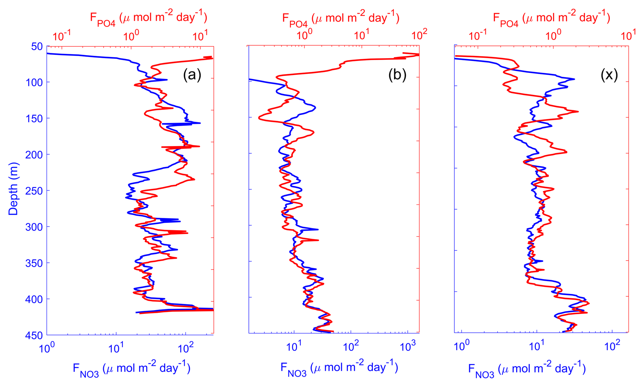
Figure 14Time average of vertical profiles of nitrate and phosphate turbulent diffusive fluxes at long-duration stations LD-A (a), LD-B (b), and LD-C (c). The scales of the nitrate and phosphate diffusive flux are set to match with the typical Redfield ratio ().
Figure 14 summarizes the main features of the turbulent diffusive fluxes with time-averaged vertical profiles. The double x axis for the nitrate and phosphate turbulent diffusive fluxes is scaled within a Redfield ratio so that the fluxes are superimposed if they follow the Redfield proportion. At depth, NO3 and PO4 fluxes follow the Redfield proportion. Closer to the surface, NO3 flux decreased: at LD-A there is a small input of nitrate in the photic layer, while at the eastern stations the nitrate flux vanishes above the base of the euphotic zone and reached zero before PO4 fluxes. These significant phosphate fluxes at shallower depths may potentially be fuelling nitrogen fixation, significant PO4 sources through turbulent diffusion that are likely to provide the required conditions for the growth of N2 fixers in the Melanesian Archipelago. Because phosphate availability likely sustains N2 fixation and therefore N input by N2 fixation in the WTSP, new primary production (Dugdale and Goering, 1967) might be sustained by new P (or new N including N2 fixation) in the photic zone.
5.2.3 Turbulent diffusion and the oligotrophic to ultra-oligotrophic conditions encountered during the OUTPACE cruise
The decrease in nitrate turbulent diffusive flux eastward was found to be consistent with the increasing oligotrophy and the deepening of the nitracline (Caffin et al., 2018; Moutin et al., 2018). As a result the nitrate input into the photic layer through turbulent diffusion was found to provide only a subordinate contribution to the N budget with a 1 %–8 % contribution to the new N (Caffin et al., 2018). In the Melanesian Archipelago, the input of nitrate into the photic layer represents a small contribution during the stratified period (Caffin et al., 2018) as well as on an annual timescale, with a 46 input by turbulent diffusion compared with a 642 input of N by N2 fixation Moutin et al. (2018).
In a 100 m layer starting from the top of the nitracline, the mean nitrate turbulent diffusive flux varies by a factor of 3 between the western LD station LD-A with a flux of ∼45 and the eastern LD-B and LD-C stations. The mean value obtained at LD-A is smaller than the average value obtained in the oligotrophic eastern Atlantic, ∼140 , by Lewis et al. (1986), suggesting an increased oligotrophy in the Pacific. It is typically 1 order of magnitude smaller than the values inferred further south, ∼30∘ S, by Stevens and Sutton (2012), where both larger Kz and nitrate vertical gradient are responsible for a larger nitrate turbulent diffusive flux. The comparison with Lewis et al. (1986) in the Atlantic Ocean also highlights the ultra-oligotrophy of the Pacific Ocean in the gyre compared to their counterpart in the Atlantic Ocean with diffusive fluxes at least 1 order of magnitude smaller as shown at LD-B and LD-C. The low and deep nitrate turbulent diffusive fluxes may not explain the higher primary production and N2 fixation rates observed in the upper 0–40 m Moutin et al. (2018).
The input of phosphate in the photic layer was also addressed as a possible source for sustaining the development of N2-fixing organisms. Phosphate turbulent diffusive fluxes mean values were significant in the photic layer with the exception of the easternmost station. In all cases, a few events of large fluxes driven by localized intense turbulent events were identified. The large variations in the turbulent diffusive fluxes resulting from the occurrence of strong turbulent events were thus underlined with a focus on long-duration stations (Caffin et al., 2018). This raised the question of the estimate of the turbulent input of nitrate in the photic layer when establishing C, N, and P budgets as well as the impact of turbulence intermittency on micro-organisms (Liccardo et al., 2013).
Variations within a factor of 10 of the depth-integrated ϵ were observed along the OUTPACE transect. The largest ϵ observed in the west compare well with the few measurements performed by Fernández-Castro et al. (2014, 2015) in the area during the Malaspina expedition. The range of values is comparable with 80 % of ϵ values within W kg−1 in the first 300 m below the mixed layer for the Malaspina expedition and 82 % for the OUTPACE ϵ within [30 m, 300 m] west of 180∘ longitude. Shear instability was evidenced as one main process responsible for turbulence, which is a well-known mechanism in the strongly sheared Pacific equatorial currents (Richards et al., 2015; Smyth and Moum, 2013). Richards et al. (2012) also mentioned the modulation of the turbulence level over a 3-year period with different ENSO states in the western equatorial Pacific, with a maximum shear during La Niña events compared to El Niño events. How this turbulence cycle is relevant to the OUTPACE region would be an interesting point to address with possible higher turbulence level provided that the OUTPACE cruise took place during an El Niño event. Shear instability was found to be more likely to occur in the western part of our study area, with most critical Ri encountered there. This basic analysis thus explained the contrast in dissipation observed along the transect. Whether the onset of shear instability may be driven by the low-frequency flow or the internal wave field could not be inferred from the short-duration stations, but insights into the impact of internal waves were given with estimates of the two main forcings for internal waves and the analysis of LD stations. The main forcings of internal waves were found to vary significantly along the 19∘ S longitudinal transect, thus pointing out the possible impact of internal waves on the contrast in energy dissipation. The most striking factor was related to the atmospheric forcing, with the occurrence of cyclones in the west leading to an energetic baroclinic near-inertial wave field. This internal wave component was characterized at the western long-duration station, LD-A, as well as its impact on energy dissipation. These scenarios are typically encountered in tropical regions where baroclinic near-inertial waves are known to contribute to energy dissipation in the upper ocean (Cuypers et al., 2013; Soares and Richards, 2013). The process of dissipation is often constrained by the mean subinertial flow with ray focusing or critical levels depending on the spatial structure of the flow (Soares et al., 2015; Whitt and Thomas, 2013). These mechanisms were not addressed here, but will be the focus of a future study using observations at the LD-A site. The context of the OUTPACE cruise with significant niw generated by a cyclone is very specific, of general interest for the studied region, where these meteorological phenomena are frequent at the end of the summer. It hides the more continuous influence of internal tides as a turbulence driver. Our measurements show only a slightly larger semi-diurnal kinetic energy in the west at LD-A compared to LD-B and LD-C, but suggest a larger contrast in shear variance.
The impact of turbulence on biogeochemical fluxes and trophic gradients was estimated based on nitrate and phosphate turbulent diffusive fluxes. The nitrate input into the photic layer through turbulent diffusion was found to provide only a subordinate contribution to the N budget as a result of the eastward decrease in nitrate turbulent diffusive fluxes and the deepening of the nitracline. New production is mainly supported by N2 fixation and is located in the western tropical South Pacific. The higher phosphate turbulent fluxes compared to nitrate fluxes provide an excess P relative to Redfield stoichiometry and a potential ecological niche for N2 fixing organisms in the west. In addition to the lower iron availability in the east preventing N2 fixation from occurring, the high iron availability in the west allows this process and the excess P provided to the photic zone to sustain a higher new primary production, explaining the western–eastern oligotrophy gradient.
All data and metadata are available at the French INSU/CNRS LEFE CYBER database (scientific coordinator: Hervé Claustre; data manager and webmaster: Catherine Schmechtig) at the following web address: http://www.obs-vlfr.fr/proof/php/outpace/outpace.php (last access: 21 December 2018, INSU/CNRS LEFE CYBER, 2017).
The authors declare that they have no conflict of interest.
This article is part of the special issue “Interactions between planktonic organisms and biogeochemical cycles across trophic and N2 fixation gradients in the western tropical South Pacific Ocean: a multidisciplinary approach (OUTPACE experiment)”. It is not associated with a conference.
This is a contribution of the OUTPACE (Oligotrophy from
UlTra-Oligotrophy PAcific
Experiment) project (https://outpace.mio.univ-amu.fr, last access: 12
December 2018) funded by the French research national agency
(ANR-14-CE01-0007-01), the LEFE-CyBER programme (CNRS-INSU), the GOPS
programme (IRD), and the CNES (BC T23, ZBC 45000048836). We warmly
acknowledge the assistance of the crew of the French research vessel
l'Atalante during the deployment of the VMP. We thank
Olivier Desprez for his technical support and help during the cruise. The
microstructure profiler was funded through the ANR OUTPACE
project.
Edited by: Laurent
Mémery
Reviewed by: Bieito Fernández-Castro and one
anonymous referee
Alford, M. H.: Improved global maps and 54-year history of wind-work on ocean inertial motions, Geophys. Res. Lett., 30, 1424, https://doi.org/10.1029/2002GL016614, 2003. a, b
Alford, M. H. and Zhao, Z.: Global patterns of low-mode internal-wave propagation – Part I: Energy and Energy Flux, J. Phys. Oceanog., 37, 1829–1848, 2007. a, b
Alford, M. H. and Zhao, Z.: Global patterns of low-mode internal-wave propagation – Part II: Group velocity, J. Phys. Oceanogr., 37, 1849–1858, 2007.
Amante, C. and Eakins, B. W.: ETOPO1 1 Arc-Minute Global Relief Model: Procedures, Data Sources and Analysis, NOAA Technical Memorandum NESDIS NGDC-24, National Geophysical Data Center, NOAA, https://doi.org/10.7289/V5C8276M, 2009. a
Ascani, F., Richards, K. J., Firing, E., Grant, S., Johnson, K. S., Jia, Y., Lukas, R., and Karl, D. M.: Physical and biological controls of nitrate concentrations in the upper subtropical North Pacific Ocean, Deep-Sea Res. Pt. II, 93, 119–134, 2013. a
Baines, P.: On internal tide generation models, Deep-Sea Res. Pt I, 29, 307–338, 1982. a
Blain, S., Quéguiner, B., Armand, L., et al.: Effect of natural iron fertilization on carbon sequestration in the Southern Ocean, Nature, 446, 1070, https://doi.org/10.1038/nature05700, 2007 a
Bonnet, S., Caffin, M., Berthelot, H., and Moutin, T.: Hot spot of N2 fixation in the western tropical south pacific pleads for a spatial decoupling between N2 fixation and denitrification, P. Natl. Acad. Sci. USA, 114, E2800–E2801, 2017. a, b
Bonnet, S., Guieu, C., Bruyant, F., Prášil, O., Van Wambeke, F., Raimbault, P., Moutin, T., Grob, C., Gorbunov, M. Y., Zehr, J. P., Masquelier, S. M., Garczarek, L., and Claustre, H.: Nutrient limitation of primary productivity in the Southeast Pacific (BIOSOPE cruise), Biogeosciences, 5, 215-225, https://doi.org/10.5194/bg-5-215-2008, 2008. a
Bouffard, D. and Boegman, L.: A diapycnal diffusivity model for stratified environmental flows, Dynam. Atmos. Oceans, 61, 14–34, 2013. a, b
Caffin, M., Moutin, T., Foster, R. A., Bouruet-Aubertot, P., Doglioli, A. M., Berthelot, H., Guieu, C., Grosso, O., Helias-Nunige, S., Leblond, N., Gimenez, A., Petrenko, A. A., de Verneil, A., and Bonnet, S.: N2 fixation as a dominant new N source in the western tropical South Pacific Ocean (OUTPACE cruise), Biogeosciences, 15, 2565–2585, https://doi.org/10.5194/bg-15-2565-2018, 2018. a, b, c, d, e, f, g, h, i
Cuypers, Y., Le Vaillant, X., Bouruet-Aubertot, P., Vialard, J., and Mcphaden, M. J.: Tropical storm-induced near-inertial internal waves during the cirene experiment: Energy fluxes and impact on vertical mixing, J. Geophys. Res.-Oceans, 118, 358–380, 2013. a
de Verneil, A., Rousselet, L., Doglioli, A. M., Petrenko, A. A., and Moutin, T.: The fate of a southwest Pacific bloom: gauging the impact of submesoscale vs. mesoscale circulation on biological gradients in the subtropics, Biogeosciences, 14, 3471–3486, https://doi.org/10.5194/bg-14-3471-2017, 2017. a, b
Diamond, H. J., Lorrey, A. M., and Renwick, J. A.: A southwest Pacific tropical cyclone climatology and linkages to the El Niño–Southern Oscillation, J. Climate, 26, 3–25, 2013. a
Dugdale, R. and Goering, J.: Uptake of new and regenerated forms of nitrogen in primary productivity, Limnol. Oceanogr., 12, 196–206, 1967. a
Dupouy, C., Neveux, J., Subramaniam, A., Mulholland, M. R., Montoya, J. P., Campbell, L., Carpenter, E. J., and Capone, D. G.: Satellite Captures Trichodesmium Blooms in the southwestern Tropical Pacific, EOS, 81, 13–16, 2000. a
Egbert, G. D. and Erofeeva, S. Y.: Efficient inverse modeling of barotropic ocean tides, J. Atmos. Ocean. Tech., 19, 183–204, 2002. a
Fernández-Castro, B., Mouriño-Carballido, B., Benítez-Barrios, V., Chouciño, P., Fraile-Nuez, E., Graña, R., Piedeleu, M., and Rodríguez-Santana, A.: Microstructure turbulence and diffusivity parameterization in the tropical and subtropical Atlantic, Pacific and Indian Oceans during the Malaspina 2010 expedition, Deep-Sea Res. Pt I, 94, 15–30, 2014. a, b, c
Fernández-Castro, B., Mouriño-Carballido, B., Marañón, E., Chouciño, P., Gago, J., Ramírez, T., Vidal, M., Bode, A., Blasco, D., Royer, S.-J., Estrada, M., and Simó, R.: Importance of salt fingering for new nitrogen supply in the oligotrophic ocean, Nat. Commun., 6, 8002, https://doi.org/10.1038/ncomms9002, 2015. a, b
Ferron, B., Kokoszka, F., Mercier, H., and Lherminier, P.: Dissipation rate estimates from microstructure and finescale internal wave observations along the A25 Greenland-Portugal OVIDE line, J. Atmos. Ocean. Tech., 31, 2530–2543, 2014. a, b
Gill, A.: On the behavior of internal waves in the wakes of storms, J. Phys. Oceanogr., 14, 1129–1151, 1984. a, b
Gregg, M., Peters, H., Wesson, J., Oakey, N., and Shay, T.: Intensive measurements of turbulence and shear in the equatorial undercurrent, Nature, 318, 140-144, 1985. a
Guidi, L., Calil, P. H. R., Duhamel, S., Björkman, K. M., Doney, S. C., Jackson, G. A., Li, B., Church, M. J., Tozzi, S., Kolber, Z. S., Richards, K. J., Fong, A. A., Letelier, R. M., Gorsky, G., Stemman, L., and Karl, D. M.: Does eddy-eddy interaction control surface phytoplankton distribution and carbon export in the north pacific subtropical gyre?, J. Geophys. Res.-Biogeo., 117, G02024, https://doi.org/10.1029/2012JG001984, 2012. a
Guieu, C., Bonnet, S., Petrenko, A., Menkes, C., Chavagnac, V., Desboeufs, K., Maes, C., and Moutin, T.: Iron from a submarine source impacts the productive layer of the Western Tropical South Pacific (WTSP), Sci. Rep., 8, 9075, https://doi.org/10.1038/s41598-018-27407-z, 2018. a
Herbland, A. and Voituriez, B.: Production primaire, nitrate et nitrite dans l'Atlantique tropical: 1. Distribution du nitrate et production primaire, Cah. ORSTOM. Série Océanographie, 15, 47–55, 1977. a
INSU/CNRS LEFE CYBER: OUTPACE, Oligotrophy to UlTra-oligotrophy PACific Experiment, Data and Metadata, available at: http://www.obs-vlfr.fr/proof/php/outpace/outpace.php (last access: 21 December 2018), 2017. a
Klemp, J. B., Skamarock, W. C., and Dudhia, J.: Conservative split-explicit time integration methods for the compressible nonhydrostatic equations, Mon. Weather Rev., 135, 2897–2913, 2007. a
Ledwell, J. R., McGillicuddy Jr., D. J., and Anderson, L. A.: Nutrient flux into an intense deep chlorophyll layer in a mode-water eddy, Deep-Sea Res. Pt. II, 55, 1139–1160, 2008. a
Lewis, M. R., Hebert, D., Harrison, W. G., Platt, T., and Oakey, N. S.: Vertical nitrate flux in the oligotrophic ocean, Science, 234, 870–873, 1986. a, b
Liccardo, A., Fierro, A., Iudicone, D., Bouruet-Aubertot, P., and Dubroca, L.: Response of the deep chlorophyll maximum to fluctuations in vertical mixing intensity, Prog. Oceanogr., 109, 33–46, 2013. a
Liu, L. L., Wang, W., and Huang, R. X.: The mechanical energy input to the ocean induced by tropical cyclones, J. Phys. Oceanogr., 38, 1253–1266, 2008. a
Moutin, T. and Bonnet, S.: Outpace cruise, rv l'atalante, French Oceanographic Cruises, https://doi.org/10.17600/15000900, 2015. a
Moutin, T. and Prieur, L.: Influence of anticyclonic eddies on the Biogeochemistry from the Oligotrophic to the Ultraoligotrophic Mediterranean (BOUM cruise), Biogeosciences, 9, 3827–3855, https://doi.org/10.5194/bg-9-3827-2012, 2012. a
Moutin, T., Doglioli, A. M., de Verneil, A., and Bonnet, S.: Preface: The Oligotrophy to the UlTra-oligotrophy PACific Experiment (OUTPACE cruise, 18 February to 3 April 2015), Biogeosciences, 14, 3207–3220, https://doi.org/10.5194/bg-14-3207-2017, 2017. a, b, c, d, e
Moutin, T., Karl, D. M., Duhamel, S., Rimmelin, P., Raimbault, P., Van Mooy, B. A. S., and Claustre, H.: Phosphate availability and the ultimate control of new nitrogen input by nitrogen fixation in the tropical Pacific Ocean, Biogeosciences, 5, 9500109, https://doi.org/10.5194/bg-5-95-2008, 2008. a, b, c
Moutin, T., Wagener, T., Caffin, M., Fumenia, A., Gimenez, A., Baklouti, M., Bouruet-Aubertot, P., Pujo-Pay, M., Leblanc, K., Lefevre, D., Helias Nunige, S., Leblond, N., Grosso, O., and de Verneil, A.: Nutrient availability and the ultimate control of the biological carbon pump in the western tropical South Pacific Ocean, Biogeosciences, 15, 2961–2989, https://doi.org/10.5194/bg-15-2961-2018, 2018. a, b, c, d, e
Nasmyth, P. W.: Oceanic turbulence, University of British Columbia, 1970. a
Osborn, T.: Estimates of the local rate of vertical diffusion from dissipation measurements, J. Phys. Oceanogr., 10, 83–89, 1980. a
Price, J. F.: Internal wave wake of a moving storm. Part I. Scales, energy budget and observations, J. Phys. Oceanogr., 13, 949–965, 1984. a
Richards, K., Kashino, Y., Natarov, A., and Firing, E.: Mixing in the western equatorial Pacific and its modulation by ENSO, Geophys. Res. Lett., 39, L02604, https://doi.org/10.1029/2011GL050439, 2012. a
Richards, K. J., Natarov, A., Firing, E., Kashino, Y., Soares, S. M., Ishizu, M., Carter, G. S., Lee, J. H., and Chang, K. I.: Shear-generated turbulence in the equatorial Pacific produced by small vertical scale flow features, J. Geophys. Res.-Oceans, 120, 3777–3791, 2015. a, b
Rousselet, L., de Verneil, A., Doglioli, A. M., Petrenko, A. A., Duhamel, S., Maes, C., and Blanke, B.: Large- to submesoscale surface circulation and its implications on biogeochemical/biological horizontal distributions during the OUTPACE cruise (southwest Pacific), Biogeosciences, 15, 2411–2431, https://doi.org/10.5194/bg-15-2411-2018, 2018. a, b, c
Shih, L. H., Koseff, J. R., Ivey, G. N., and Ferziger, J. H.: Parameterization of turbulent fluxes and scales using homogeneous sheared stably stratified turbulence simulations, J. Fluid Mech., 525, 193–214, 2005. a, b
Skamarock, W. C., William, C., Klemp, J. B., Dudhia, J., Gill, D. O., Barker, D. M., Wang, W., and Powers, J. G.: A description of the advanced research WRF version 2, National Center For Atmospheric Research, Tech. Note, 2005 a, b
Smyth, W. D. and Moum, J. N.: Marginal instability and deep cycle turbulence in the eastern equatorial Pacific Ocean, Geophys. Res. Lett., 40, 6181–6185, https://doi.org/10.1002/2013GL058403, 2013. a, b
Soares, S. and Richards, K.: Radiation of inertial kinetic energy as near-inertial waves forced by tropical Pacific Easterly waves, Geophys. Res. Lett., 40, 1760–1765, 2013. a
Soares, S. M., Richards, K. J., and Natarov, A.: Near inertial waves in the tropical Indian Ocean: Energy fluxes and dissipation, American Geophysical Union, Ocean Sciences Mtg., Honolulu HI, 2014.
Soares, S. M., Richards, K. J., and Natarov, A.: Near inertial waves in the tropical Indian Ocean: Energy fluxes and dissipation during CINDY, J. Geophys. Res., 121, 3297–3324, https://doi.org/10.1002/2015JC011600, 2015. a, b
St Laurent, L., Simmons, H., and Jayne, S.: Estimating tidally driven mixing in the deep ocean, Geophys. Res. Lett., 29, 2106–2109, 2002. a
Stevens, C. L. and Sutton, P. J.: Internal waves downstream of Norfolk Ridge, western Pacific, Limnol. Oceanogr., 57, 897–911, 2012. a
Sun, C., Smyth, W. D., and Moum, J. N.: Dynamic instability of stratified shear flow in the upper equatorial Pacific, J. Geophys. Res.-Oceans, 103, 10323–10337, 1998. a
Visbeck, M.: Deep velocity profiling using Lowered Acoustic Doppler Current Profilers: Bottom track and inverse solutions, J. Atmos. Ocean. Tech., 19, 794–807, 2002. a
Whalen, C., Talley, L., and MacKinnon, J.: Spatial and temporal variability of global ocean mixing inferred from argo profiles, Geophys. Res. Lett., 39, L18612, https://doi.org/10.1029/2012GL053196, 2012. a
Whitt, D. B. and Thomas, L. N.: Near-inertial waves in strongly baroclinic currents, J. Phys. Oceanogr., 43, 706–725, 2013. a
- Abstract
- Introduction
- Data and methods
- Spatial pattern of turbulence
- Possible impact of internal waves: focus on long-duration stations
- Impact of turbulence on biogeochemical fluxes: spatial pattern and intermittency
- Conclusions
- Data availability
- Competing interests
- Special issue statement
- Acknowledgements
- References
upliftnutrients into the euphotic layer. The origin of the turbulence that was found contrasted along the transect was also determined.
- Abstract
- Introduction
- Data and methods
- Spatial pattern of turbulence
- Possible impact of internal waves: focus on long-duration stations
- Impact of turbulence on biogeochemical fluxes: spatial pattern and intermittency
- Conclusions
- Data availability
- Competing interests
- Special issue statement
- Acknowledgements
- References