the Creative Commons Attribution 4.0 License.
the Creative Commons Attribution 4.0 License.
 | 13 Dec 2018
Quantitative mapping and predictive modeling of Mn nodules' distribution from hydroacoustic and optical AUV data linked by random forests machine learning
Timm Schoening
Evangelos Alevizos
Jens Greinert
In this study, high-resolution bathymetric multibeam and optical image data, both obtained within the Belgian manganese (Mn) nodule mining license area by the autonomous underwater vehicle (AUV) Abyss, were combined in order to create a predictive random forests (RF) machine learning model. AUV bathymetry reveals small-scale terrain variations, allowing slope estimations and calculation of bathymetric derivatives such as slope, curvature, and ruggedness. Optical AUV imagery provides quantitative information regarding the distribution (number and median size) of Mn nodules. Within the area considered in this study, Mn nodules show a heterogeneous and spatially clustered pattern, and their number per square meter is negatively correlated with their median size. A prediction of the number of Mn nodules was achieved by combining information derived from the acoustic and optical data using a RF model. This model was tuned by examining the influence of the training set size, the number of growing trees (ntree), and the number of predictor variables to be randomly selected at each node (mtry) on the RF prediction accuracy. The use of larger training data sets with higher ntree and mtry values increases the accuracy. To estimate the Mn-nodule abundance, these predictions were linked to ground-truth data acquired by box coring. Linking optical and hydroacoustic data revealed a nonlinear relationship between the Mn-nodule distribution and topographic characteristics. This highlights the importance of a detailed terrain reconstruction for a predictive modeling of Mn-nodule abundance. In addition, this study underlines the necessity of a sufficient spatial distribution of the optical data to provide reliable modeling input for the RF.


High-resolution quantitative predictive mapping of the distribution and abundance of manganese nodules (Mn nodules) is of interest for both the deep-sea mining industry and scientific fields such as marine geology, geochemistry, and ecology. The distribution and abundance of Mn nodules are affected by several factors such as local bathymetry (Craig, 1979; Kodagali, 1988; Kodagali and Sudhakarand, 1993; Sharma and Kodagali, 1993), sedimentation rate (Glasby, 1976; Frazer and Fisk, 1981; von Stackelberg and Beiersdorf, 1991; Skornyakova and Murdmaa, 1992), availability of nucleus material (Glasby, 1973), and bottom current strength (Frazer and Fisk, 1981; Skornyakova and Murdmaa, 1992). As a consequence, the distribution and abundance of Mn nodules is heterogeneous (Craig, 1979; Frazer and Fisk, 1981; Kodagali, 1988; Kodagali and Sudhakar, 1993; Kodagali and Chakraborty, 1999; Kuhn et al., 2011), even on fine scales of 10 to 1000 m (Peukert et al., 2018a; Alevizos et al., 2018). This increases the difficulty of quantitative predictive mapping using remote-sensing methods. Vast areas of the seafloor can be mapped by ship-mounted, multibeam echo-sounder systems (MBESs). State-of-the-art MBESs feature a low frequency (12 kHz) and can map ca. 300 km2 of seafloor in 4500 m water depth per hour. Hence, low-resolution regional maps can be created at a grid cell size of 50 to 100 m within which the main Mn-nodule occurrence can become apparent, based on the backscatter intensity (Kuhn et al., 2011; Rühlemann et al., 2011; Jung et al., 2001). A general separation in areas of high and low abundance (kg m−2) of Mn nodules seems possible, especially in flat areas where sedimentological changes and physical influences on the footprint size and incidence angle of the transmitted acoustic pressure wave can be corrected accurately (De Moustier, 1986; Kodagali and Chakraborty, 1999; Chakraborty and Kodagali, 2004; Kuhn et al., 2010, 2011; Rühlemann et al., 2011, 2013). However, the patchy distribution of Mn nodules in size and number at meter-scale cannot be resolved with ship-mounted MBES data (Petersen, 2017). For an operational resource assessment, a higher resolution of a few meters grid cell size is needed to supply accurate depth, slope, and Mn-nodule distribution variability (Kuhn et al., 2011). Supplementary to the spatial mapping by acoustic sensors, point-based measurements from box corer samples are used as ground-truth data for training and validation of geostatistical techniques (e.g., kriging) in order to create quantitative maps of Mn-nodule abundance (Mucha et al., 2013; Rahn, 2017). However, the generally low number of ground-truth samples during surveys (usually below 10), their limited sampling area (typically 0.25 m2), and the relatively large distance between them (> 1 nm) prevent an accurate correlation with the ship-based MBES data and thus a good prediction of the total Mn nodules' mass and distribution in large areas (Petersen, 2017). Importantly, the sparse sampling with box corers affects the performance of interpolation and geostatistical techniques, which are typically applied during data analysis (Li and Heap, 2011, 2014; Kuhn et al., 2016). In this article, we address this challenge by combining high-resolution hydroacoustic and optical data sets acquired with an autonomous underwater vehicle (AUV) and connecting those data with a machine learning (ML) algorithm (here random forests), in order to predict the spatial distribution of the number of Mn nodules per square meter. Unlike geostatistical methods, ML can be used to incorporate information from different bathymetric derivative layers and to detect complex relationships among predictor variables without making any prior assumptions about the type of their relationship or value distribution (Garzn et al., 2006; Lary et al., 2016). To this end, first predictions have already been achieved (Knobloch et al., 2017; Vishnu et al., 2017; Alevizos et al., 2018). Here, we present a complete data analysis workflow for potential mining exploration (Fig. 1).

Figure 1Schematic workflow of the data sets used in this study to enable the spatial assessment of Mn nodules inside the study area. The medium resolution of AUV MBES (meter scale) refers to the comparison of the optical and physical data (centimeter scale).
1.1 AUV hydroacoustic mapping
AUVs have proven their usefulness for multibeam data acquisition in the deep-sea environment (Grasmueck et al., 2006; Deschamps et al., 2007; Haase et al., 2009; Wynn et al., 2014; Clague et al., 2014, 2018; Pierdomenico et al., 2015; Peukert et al., 2018a). They achieve higher spatial and vertical resolution compared to ship-mounted MBESs. This is due to their operation close to the seafloor, which results in a smaller footprint at a given beam angle and enables the use of higher frequencies (Henthorn et al., 2006; Mayer, 2006; Caress et al., 2008; Paduan et al., 2009). Additionally, AUVs avoid problems like near-surface turbulences, bubbles, ship noise, and strong sound velocity changes (Kleinrock et al., 1992a, b; Jakobson et al., 2016; Paul et al., 2016). They work independently from the surface vessel and operate at a stable altitude. AUVs can efficiently conduct a dive pattern of dense survey lines and thus reduce survey effort and costs (Chance et al., 2000; Bellingham, 2001; Bingham et al., 2002; Danson, 2003; Roman and Mather, 2010). High-resolution bathymetry enables computing bathymetric derivatives like slope and rugosity with a similarly high resolution. These derivatives play an important role in predicting Mn nodules' distribution and abundance (Craig, 1979; Kodagali, 1988; Skornyakova and Murdmaa, 1992; Kodagali and Sudhakar, 1993, Sharma and Kodagali, 1993; Ko et al., 2006). However, a small number of recent studies have investigated this role on an AUV scale (Okazaki and Tsune, 2013; Peukert et al., 2018a; Alevizos et al., 2018).
1.2 Underwater optical data
Underwater optical data have generally played an important role in the qualitative analysis of the seafloor features and for the specific task of assessing Mn nodules' distribution explicitly (Glasby, 1973; Rogers, 1987; Skornyakova and Murdmaa, 1992; Sharma et al., 1993). The development of automated detection algorithms enabled quantitative optical image data analysis and subsequent statistical interpretation of Mn-nodule densities. The spatial coverage of optical imaging is much higher than for box core sampling. The data resolution remains high enough to reveal the high variance in the spatial distribution of nodules at meter scale. Thus optical data can fill the investigation gap between ground-truth sampling and hydroacoustic remote sensing (Sharma et al., 2010, 2013; Schoening et al., 2012a, 2014, 2015, 2016, 2017a; Kuhn and Rathke, 2017). Moreover, mosaicking of optical data could reveal mining obstacles such as outcropping basements or volcanic pillow lava flows. In addition, seafloor photos are the source for evaluating benthic fauna occurrences and related habitats on a wider area (Schoening et al., 2012b; Durden et al., 2016).
1.3 Box corer sampling
Box coring is common to obtain physical samples of Mn nodules and sediments for resource assessments and biological studies. While optical data reveal only the exposed and semi-buried Mn nodules, box corers collect the top 30–50 cm of the seafloor with minimum disturbance, allowing an accurate measure of the Mn nodules' abundance (kg m−2). Box coring data are used for training and validation in geostatistical methods for quantitative and spatial predictions of Mn nodules (e.g., Mucha et al., 2013; Knobloch et al., 2017). The representativeness of box coring data is disputable as few deployments can be made due to time constraints (ca. 4 h per core) and as the spatial coverage of one sample is rather low (ca. 0.25 m2).
1.4 Random forests
Random forests (RF) is an ensemble machine learning (ML) method composed of multiple weaker learners, namely classification or regression trees (Breiman, 2001a). Within RF an ensemble of distinct tree models is trained using a random subsample of the training data for each tree until a maximum tree size is reached. In each tree, each node is split using the best among a subset of predictors randomly chosen at that node instead of using the best split among all variables (Liaw and Wiener, 2002). Thus, the process is double-randomized which further reduces the correlation between trees. About two-thirds of the training data are used to tune the RF while the remaining “out-of-bag” (OOB) samples are used for an internal validation. By aggregating the predictions of all trees (majority votes for classification, the average for regression), new values can be predicted. This aggregation keeps the bias low while it reduces the variance, resulting in a more powerful and accurate model. RFs have the ability to estimate the importance of each predictor variable, which enables data mining of the high-dimensional prediction data. Terrestrial studies use RFs in prospectivity mapping of mineral deposits (Carranza and Laborte, 2015a, b; 2016; Rodriguez-Galiano et al., 2014, 2015). In the marine environment, RFs have been used to combine MBES bathymetry, backscatter, their derivatives, sediment sampling, and optical data for various seabed classification and regression tasks (e.g., Li et al., 2010, 2011a; Che Hasan et al., 2014; Huang et al., 2014). Further studies showed the robustness of RFs for selected data sets compared to other ML algorithms (Che Hasan et al., 2012; Stephens and Diesing, 2014; Diesing and Stephens, 2015; Herkul et al. 2017), as well as to geostatistical and deterministic interpolation methods (Li et al., 2010, 2011a, b; Diesing et al., 2014).
The study area lies in the Clarion–Clipperton Zone (CCZ; ca. 4×10⁶ km2) in the eastern central Pacific Ocean. The CCZ has triggered scientific and industrial interest for several decades due to its high resource potential in Mn-nodule deposits (Hein et al., 2013; Petersen et. al., 2016) with an average nodule abundance of 15 kg m−2 (SPC, 2013). At the time of writing, the International Seabed Authority (ISA) has granted 17 exploration licences inside the CCZ (Fig. 2a). The study area described here is part of the Belgian GSR (Global Sea Mineral Resources) license area (Fig. 2b) and will be referred to as block G77 (Fig. 2c). Overall, this part of the Belgian license area has a high bathymetric range and complex morphology, due to the presence of submarine volcanoes, solitary seamounts, and seamount chains. Block G77 is characterized by a low bathymetric range (77 m) and mostly gentle slopes (95 % of the area below 5∘). An exception is located in the eastern part, where subrecent small-scale volcanic activity created 15 cone-shaped morphological features of up to 55 m height and 150 m width that are clustered in an area of ca. 700 m × 380 m. Despite the gentle slopes, block G77 is characterized by an uneven microrelief (according to Dikau, 1990) especially in the western part, where small (2–4 m) depressions coexist next to short (2–4 m) protrusions. In the central part, a 30 m high elevation acts as a natural barrier between the western part of the study area that features more relief and the eastern part that is deeper and has less relief (Fig. 2c).
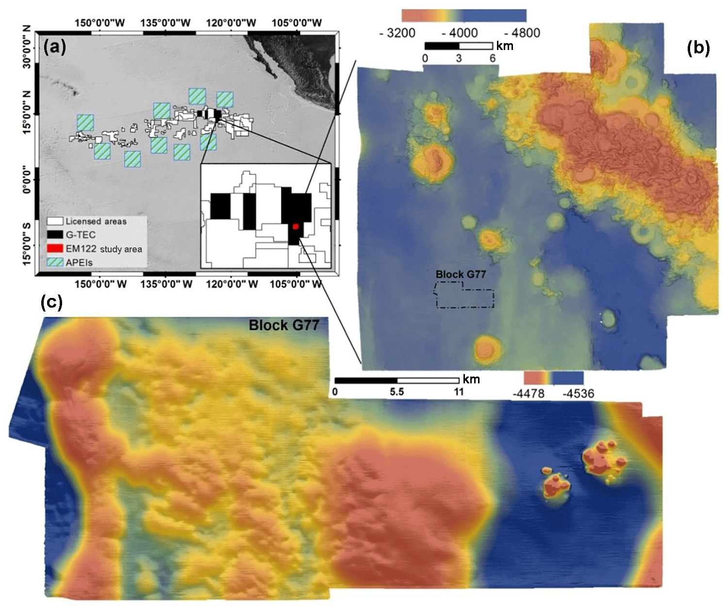
Figure 2(a) Areas of Particular Environmental Interest (APEIs), licensed areas (white), and the Belgium/GSR licenses area (black) within the CCZ. (b) Regional bathymetric map of the study area, created by the EM 122 MBES on R/V Sonne (cruise SO239). (c) Block G77, mapped by AUV Abyss with a Teledyne Reson Seabat 7125 MBES.
3.1 Hydroacoustic data acquisition and post-processing
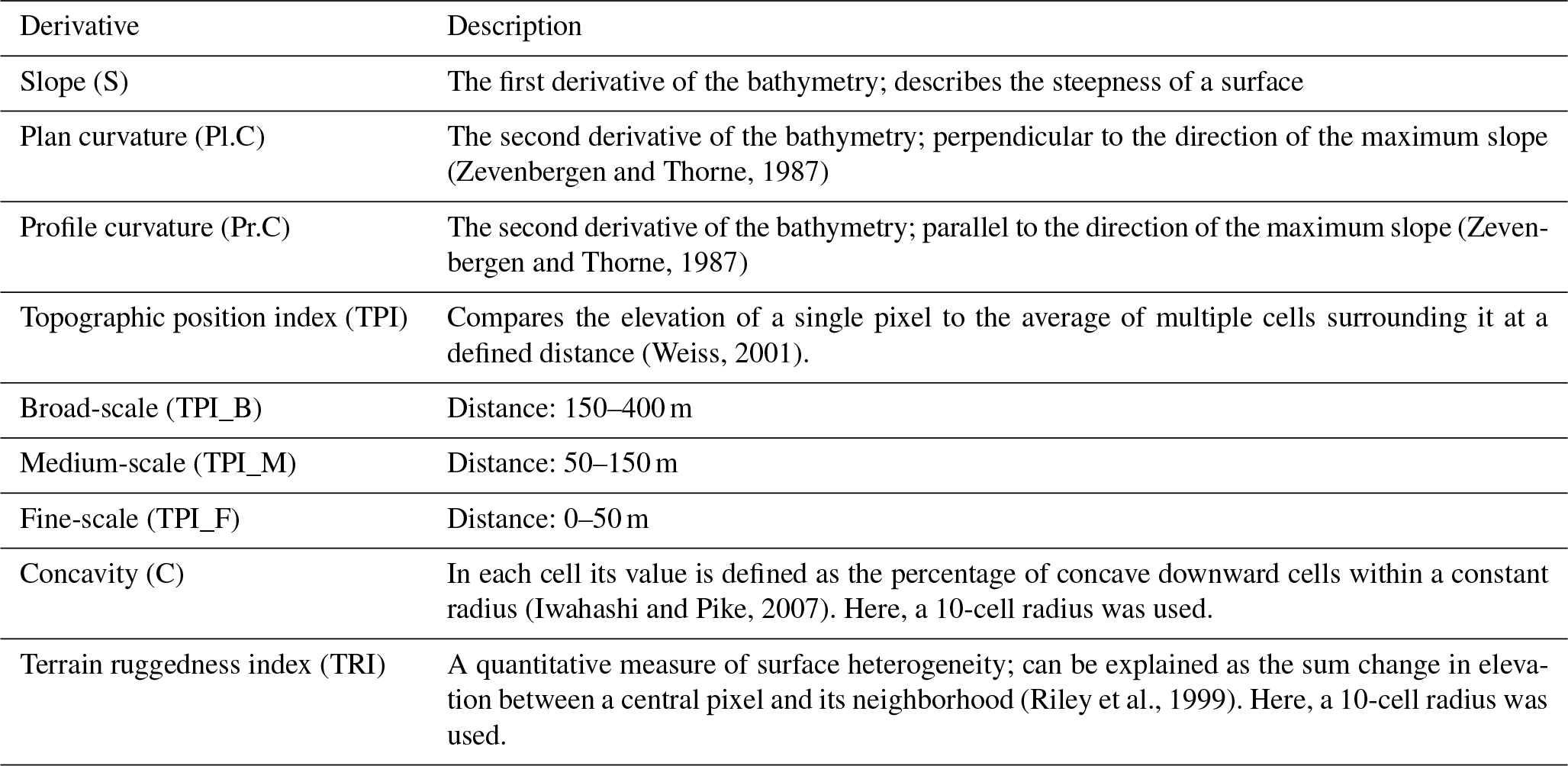
The data (Greinert, 2016) were collected in March 2015 during cruise SO239 EcoResponse (Martínez Arbizu and Haeckel, 2015) with the German research vessel Sonne. Ship-based mapping was conducted with a hull-mounted Kongsberg EM 122 MBES (12 kHz, 0.5∘ along- and 1∘ across-track beam angle, 432 beams with 120∘ swath angle). High-resolution MBES data were acquired with AUV Abyss (GEOMAR, 2016) inside block G77 equipped with a Teledyne Reson Seabat 7125 MBES (200 kHz, 2∘ along- and 1∘ across-track beam angle, 256 beams with 130∘ swath angle). The data (60 km of survey lines) were acquired from 50 m altitude and with 100 % swath overlap resulting in an insonification of 9.5 km2. Post-processing of the AUV data was conducted with the Teledyne PDS2000 software for data conversion of the raw data into s7k and GSF format. Further multibeam processing (sound velocity calibration, pitch/roll/yaw/latency artifacts correction) was performed using the Qimera™ software. The largest uncertainties during AUV operations result from inaccurate navigation and localization in the deep-sea environment (Paull et al., 2014). AUV Abyss has a combination of five different systems for navigation and positioning: Global Positioning System (GPS) when at the sea surface, Doppler velocity log (DVL) when 100 m or less from the ground, inertial navigation system (INS), long baseline acoustic navigation (LBL), and dead reckoning (GEOMAR, 2016). Each system has its own limitations that contribute to the total navigation error (Sibenac et al., 2004; Chen et al., 2013) that generally results in positioning drifts over time. Consequently, this affects the position accuracy of the MBES and optical data. Our AUV MBES data processing and an absolute geo-referencing of the resulting AUV bathymetry grid with the EM122 ship data, supplemented with the use of MBnavadjust in MB-Systems (Caress et al., 2017), resulted in a well-calibrated AUV bathymetric data set. The position of the AUV image data “only” relies on the abovementioned sensors with a “small” position error that is not quantifiable. Backscatter data were excluded from the modeling procedure due to artifacts and a generally poor quality. The output grid cell size for the analyses was set to 3 m × 3 m. The depth raster was exported as ASCII format for further analysis in SAGA GIS v.6.3.0. SAGA includes numerous tools that focus on terrain analysis (Conrad, 2015). Eight bathymetric derivatives were computed (Table 1) with the SAGA algorithms (Appendix A).
Table 1The bathymetric derivatives computed in SAGA GIS and used as predictor variables.
3.2 Optical data acquisition and post-processing
High-resolution optical data (20.2 megapixels) were acquired by the DeepSurveyCamera system on board AUV Abyss (Kwasnitschka et al., 2016). During image acquisition, the altitude above ground was 5 to 11 m, resulting in an overlap between the images of ca. 60 % in each direction. In total, 11 276 photos were acquired in block G77 (Greinert, 2017) and analyzed with the automated image analysis algorithm CoMoNoD (Schoening et al., 2017a, b, c). For each image this algorithm delineates each individual Mn nodule and provides quantitative information on each nodule (size in cm2, alignment of main axis, geographical coordinate of the nodule). This information is further aggregated per image to provide the average number of Mn nodules per square meter (Mn nodules m−2), the nodule coverage of the seafloor in percent, and the nodule size distribution in square-centimeter size quantiles. The algorithm has successfully been applied for quantitative assessment and predictive modeling of Mn nodules (Peukert et al., 2018a; Alevizos et al., 2018). Nevertheless, the derived number of Mn nodules m−2 is subject to uncertainties due to the limitations of the CoMoNoD algorithm and the nonconstant altitude of the AUV, especially in areas with slopes. The CoMoNoD algorithm cannot detect sediment-covered Mn nodules due to the low or nonexistent contrast. It may count two or more adjacent small Mn nodules as one big nodule or misinterpret benthic fauna or rock fragments with similar visual features as Mn nodules. The CoMoNoD algorithm fits an ellipsoid around each detected Mn nodule, which limits the first two disadvantages as it splits huge Mn nodules and accounts for potentially buried parts (see discussions in Schoening et al., 2017a). In general, the first two disadvantages lead to underestimations while the third one results in an overestimation of the number of Mn nodules per square meter. These limitations are common, and the need for corrections (e.g., a factor that describes the ratio between the number of Mn nodules seen in the photo and the number of nodules counted in box corers, considering for the different spatial scales) has been acknowledged (Sharma and Kodagali, 1993; Sharma et al., 2010, 2013; Tsune and Okazaki, 2014; Kuhn and Rathke, 2017). Recent studies show that the difference between image estimates and the abundance in box corer data (due to sediment covered Mn nodules) can be 2–4 times higher (Kuhn and Rathke, 2017). In this study, none of the box corers was obtained exactly at a location for which optical data exist; thus, no direct comparison and verification exist. Taking box corer samples for verification requires ultrashort baseline (USBL) navigation and imaging of the seafloor prior to the physical sampling. The effects of the nonconstant flying altitude on the detection of Mn nodules per square meter are explained in detail below. For each photo location, the depth and the bathymetric derivative values were extracted from the hydroacoustic data. As no absolute geo-referencing could be performed for the AUV-based photo surveys, drifting sensor data will have an effect on the alignment between bathymetric and photo information, which was considered while interpreting the results.
3.3 Data exploration and spatial analysis
The data exploration, spatial plotting, and analysis was performed with ArcMap™ 10.1, PAST v3.19 (Hammer et al., 2001), and R (R Development Core Team, 2008). All data were projected as a UTM Zone 10N coordinate system (to enable spatial analysis). The existence of spatial autocorrelation in the distribution of Mn nodules m−2 was examined by the global Moran's index (GMI) and Anselin local Moran's index (LMI). Both GMI (Moran, 1948, 1950) and LMI (Anselin, 1995) are well-established for examining the overall (global) and local spatial autocorrelation, respectively (e.g., Goodchild, 1986; Fu et al., 2014). GMI attains values between −1 and 1 with high positive values indicating strong spatial autocorrelation. High positive LMI index values indicate a local cluster. This cluster could be a group of observations with high–high (H–H) or low–low (L–L) values regarding the examined variable. A high negative index value implies local outliers, like high–low (H–L) or low–high (L–H) clusters, in which an observation has a higher or lower value in comparison to its adjacent observations. Both Moran's index analyses were performed in ArcMap™ 10.1 (for parameter settings see Appendix A). One decimal was retained in the presentation of the results from statistical analysis and RF modeling.
3.4 Box corer data
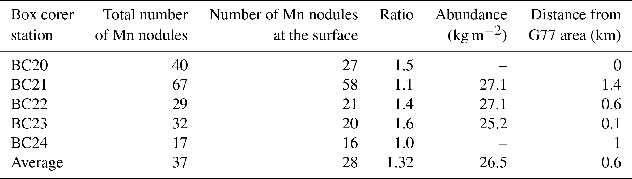
A total of five box corers (0.5 m × 0.5 m surface area) were obtained close to the study area (coordinates not given due to confidentiality). However, one is located within block G77 (Fig. 3a); this is the result of independent sampling schemes and purposes during the cruise. Nevertheless, all box core samples (maximum distance < 1.5 km) were analyzed and used for further analyses. In the three box corers, the number, size, and weight of nodules were measured and the abundance (kg m−2) was estimated (mean value: 26.5 kg m−2). The total number of Mn nodules within each box corer was compared with the number of Mn nodules on the surface resulting in an average ratio of 1.32 (Table 2). This means that ≈25 % of the nodules are not seen on the surface but are completely buried within the sediment (down to a depth of about 15 cm).
Table 2The number of Mn nodules on the sediment surface, the total number of Mn nodules per box core, the ratio of those two values, and the distance of the box corer deployments from the study area in block G77.
3.5 RF predictive modeling
The RF modeling was performed with the Marine Geospatial Ecology Tools (MGET) toolbox in ArcMap™ 10.1. MGET (Roberts et al., 2010) uses the randomForests R package for classification and regression (Liaw and Wiener, 2002). Our target variable (number of Mn nodules m−2 ) is continuous, so regression was applied. We followed the three main steps to establish a good model by selecting predictor variables, and calibration/training of the model and finally validating the model results.
Selection of predictor variables. The depth (D) and its derivatives (Table 1) were used as predictor variables. Although RFs can handle a high number of predictor variables with similar information, the exclusion of highly correlated variables can improve the RF performance and decrease computation time (Che Hasan, 2014; Li et al., 2016). Thus, the correlation between derivatives was investigated using the Spearman's rank correlation coefficient. None of the variable pairs was perfectly correlated (ρ≥95), and consequently, all of them were used for RF modeling (Appendix A).
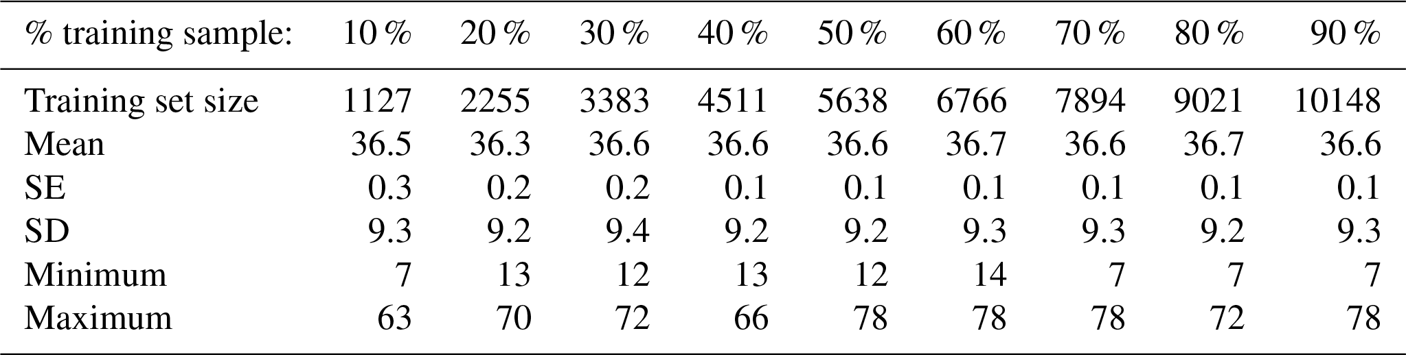
Calibration of the model. During the calibration process, the RF parameters were adjusted as follows. The number of predictor variables to be randomly selected at each node (mtry), the minimum size of the terminal nodes (nodesize), and the number of trees to grow (ntree) were set to the default values, in order to investigate the optimum training size. For regression RF the default mtry value is 1∕3 of the number of predictor variables (rounded down), nodesize is 5 and ntree is 500 (Liaw and Wiener, 2002). RF has been demonstrated to be robust regarding these parameters, and the default values have given trustworthy results (e.g., Liaw and Wiener, 2002; Diaz-Uriarte and de Andres, 2006; Cutler et al., 2007; Okun and Priisalu, 2007; Li et al., 2016, 2017). With regards to the subsampling method (replace), the subsampling without replacement was selected. Although the initial implementations of the RF algorithm use subsampling with replacement (Breiman, 2001a), later studies showed that this process might cause a biased selection of predictor variables that vary in their scale and/or in their number of categories, resulting in a biased variable importance measurement (Strobl et al., 2007, 2009; Mitchell, 2011). Based on recent findings, the raw variable importance was preferred (unscaled) as the final parameter (Diaz-Uriarte and de Andres, 2006; Strobl et al., 2008, 2009; Strobl and and Zeileis, 2008). Using these settings, the influence of the training sample size was examined (10 % to 90 % of the total sample in steps of 10 %) and compared based on the mean of squared residuals (MSR) using the respective equation provided in the randomForests R package (Liaw and Wiener, 2002). The different training groups need to be considered as representative of the total sample, in order to capture the heterogeneity of the Mn nodules' spatial distribution. The spatially random selection of subsamples by MGET ensured similar statistical characteristics in each group (Appendix A). For each case of different training sample size, the model was run 10 times and the results are presented as the average value of these 10 runs (Appendix B). Since the optimal training sample size was defined, the influence of the number of growing trees (ntree) and the influence of the number of predictor variables to be randomly selected at each node (mtry) was examined. Only for the already defined optimum training size were 10 different ntree values (100 to 1000 in steps of 100) and seven different mtry values (1 to 7 in steps of 1) tested and compared based on the MSR values. In each case of a different ntree and mtry parameter, the model was run 10 times, and the results are presented as the average value of these 10 runs (Appendix B).
Selection and external validation of the optimal model. Based on the abovementioned results and considering the sampling and computational cost, the optimal model was selected, run for 30 iterations, and applied to the entire study area. Its predicted values were validated with the observed values from the remaining data set that was not used. Several validation measures were used including the mean absolute error (MAE), the mean squared error (MSE), and the root mean squared error (RMSE). The combined use of MAE and RMSE is a well-established procedure as the MAE can evaluate better the overall performance of a model (all individual differences have equal weight), while the RMSE gives disproportionate weight to large errors showing an increased sensitivity to the presence of outliers. Due to this characteristic, RMSE is suitable for outlier detection analysis but should not be used solely as an index for the model performance (Willmott and Matsuura, 2005). Both MAE and RMSE are measured in the same unit as the data. In addition, the R2, Pearson (r), and Spearman's rank correlation coefficients were used to identify the correlation between predicted and initial values. Finally, the descriptive statistics of predicted and initial values were compared and a residual analysis was performed.
3.6 Resource assessment
As the optimal RF model was applied to the entire block G77, an estimate of the abundance (kg m−2) was computed, based on the analogy between the corresponding abundance measured from the average number of Mn nodules in the box corer data and the number of Mn nodules m−2 in each cell of the final result of the RF model. Considering that the collector can recover buried Mn nodules from a maximum depth of 10–15 cm (Sharma, 1993, 2010), the ratio of 1.32 was applied to account for Mn nodules not detected in the images, and areas with a slope of > 3∘ were excluded, assuming that a potential mining vehicle is limited to less steep slopes (UNOET, 1987).
4.1 Data exploration
The analysis of AUV photos with the CoMoNoD algorithm (Schoening et al., 2017a) revealed a rather heterogeneous pattern of Mn nodules m−2 in the study area, showing adjacent areas with high and low Mn-nodule number (Fig. 3a). The number of Mn nodules m−2 changes within less than 100 m in the overall study area and in the two main subareas b and c (Fig. 3a–c). In half of the photos (48 %), the number of Mn nodules m−2 varies from 30 to 43 with the mean value being 36.6 Mn nodules m−2. The very small change of 5 % trimmed mean value indicates the absence of extreme outliers, which is confirmed by box plot analysis (Appendix B). Further analysis of their descriptive and distribution characteristics was performed in order to assess the presence of normality in the data, with the result that the number of Mn nodules m−2 is approximately normally distributed (Appendix B). Although the presence of normality in data is not a prerequisite assumption in order to perform the RF (Breiman, 2001a), as it is with geostatistical interpolation techniques like kriging (e.g., Kuhn et al., 2016), this examination can give us a better understanding of the Mn nodules' distribution inside the study area, and it is an important step in order to examine potential extreme observations which may be derived from wrong measurements and could artificially change the training range during RF predictive modeling. Moreover, an absence of linear correlation was observed between Mn nodules m−2 and the produced bathymetric derivatives, indicating the complexity of the phenomenon (Appendix B).
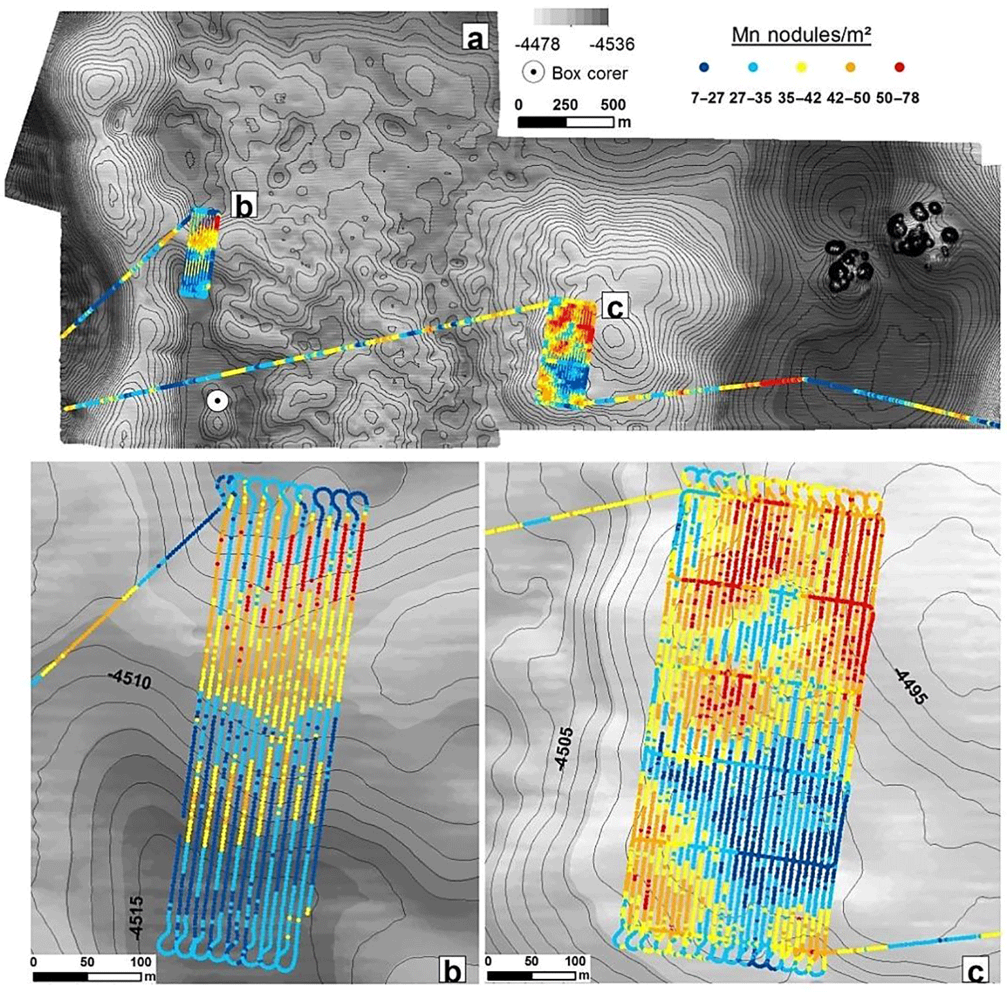
Figure 3(a) The spatial distribution of Mn nodules m−2 inside block G77 and the box corer position. (b) The spatial distribution of Mn nodules m−2 inside the subarea b. (c) The spatial distribution of Mn nodules m−2 inside the subarea c.
4.2 Spatial analyses
Spatial analyses revealed the presence of a spatial autocorrelation in the distribution of Mn nodules m−2. The GMI, with I=0.6989, p<0.01, and a Z score > 2.58 indicates a positive spatial autocorrelation. According to the incremental analysis, the index takes its highest value in the first 50 m with a gradual decrease, approaching 0 values after a distance of 400 m (Fig. 4a). Similarly, the results from the LMI show that the main size of the spatial clusters does not exceed 400 m in either direction (Fig. 5a). The main types of these clusters are H–H and L–L groups (Fig. 4b and Table 3). A distinct “buffer/transitional zone” with Mn nodules was found between these two clusters, which does not show a significant autocorrelation (Fig. 5b, c). Approximately one-third of the data does not have a significant clustering (NS). In the subarea c, the few local H–L and L–H groups are located in the outer parts of these zones without significant spatial clustering. Both H–L and L–H (from the entire study area) only account for 2.1 % of the data (Table 3). The comparison of the number of Mn nodules m−2 between the groups shows a clear discrimination between H–H and L–L clusters (Fig. 5b). The H–H clusters are in areas with 37.9–78.2 Mn nodules m−2 whilst the L–L clusters are in areas with 6.8–35.2 Mn nodules m−2.
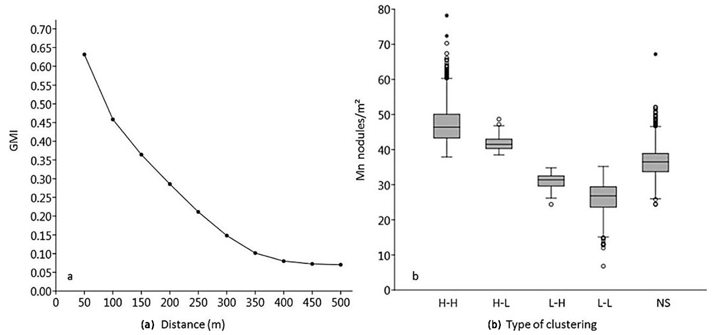
Figure 4(a) The GMI decrement due to increasing distance, after the first 50 m. (b) The range of Mn nodules m−2 in each clustered group.
Table 3Number and percentage of samples in each type of spatial clustering.
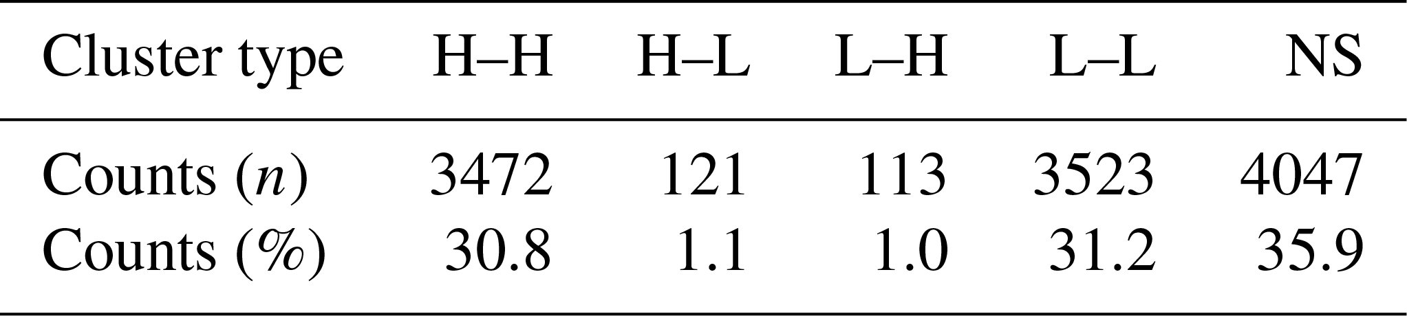
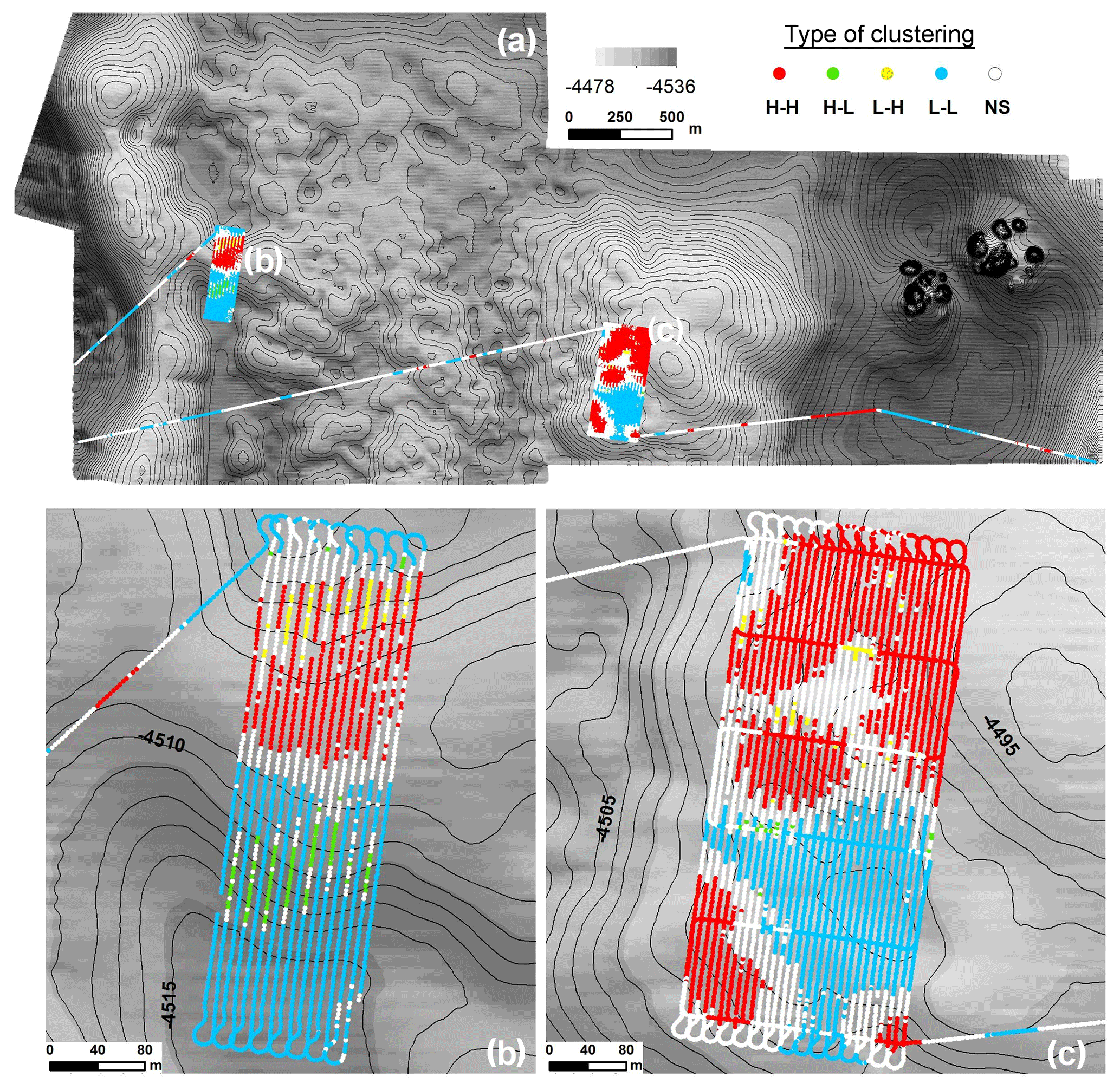
Figure 5(a) The spatial distribution of the significant cluster types inside the block G77. (b) The spatial clusters inside the subarea b. (c) The spatial clusters inside the subarea (c).
The application of the LMI reveals a bias that exists in the data due to the sampling procedure, especially in the subarea b (Fig. 5b). Here, the presence of the slope around 2.8∘ forced the AUV to vary its altitude between the ascending and descending phase (Fig. 6b). This variation seems to affect the image quality, resulting in fewer nodules being counted for higher altitudes of the AUV (Figs. 7 and 8). This is also confirmed by the distribution map of the Mn nodules m−2 (Fig. 3b). It is important to emphasize that this difference shows up clearly in the LMI results (Fig. 5b) and not in the distribution map (Fig. 3b); here the arbitrary choice of color scale can hide this bias during plotting. The comparison of the detected Mn nodules m−2 in these adjacent lines, inside the small subarea b, gives a ratio ≈1.4 between photos that have been acquired at 7–9 m altitude and those at 9–11 m altitude. The ratio is higher (≈1.8) between photos from 5–7 and 9–11 m altitude. In contrast, the ratio between photos from 5–7 m altitude and those at 7–9 m altitude is ≈1.25, indicating that the problem mainly exists at upper and lower flying altitudes. Despite their different ratio, none of these groups contain extremely high or low values of Mn nodules m−2. Moreover, in several parts of the block, the photos from higher altitude are the only source of information without the ability for further comparison, and consequently, they cannot be excluded from the modeling procedure.
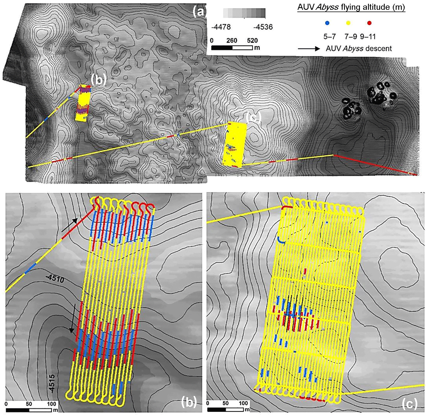
Figure 6(a) The altitude of AUV Abyss inside block G77. (b) The altitude inside the small subarea b, where the presence of the slope forces the AUV to modify its altitude, flying closer to the seafloor in the ascending phase (blue lines) and farther from the seafloor in the descending phase (red lines). (c) In the big subarea c, the AUV flying altitude is mainly constant between 7–9 m for the entire part.
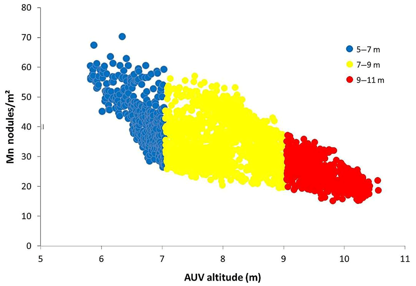
Figure 7Scatterplot of the AUV altitude (m) and the estimated number of Mn nodules m−2 inside subarea b. The colors correspond to the color scale in Fig. 7.
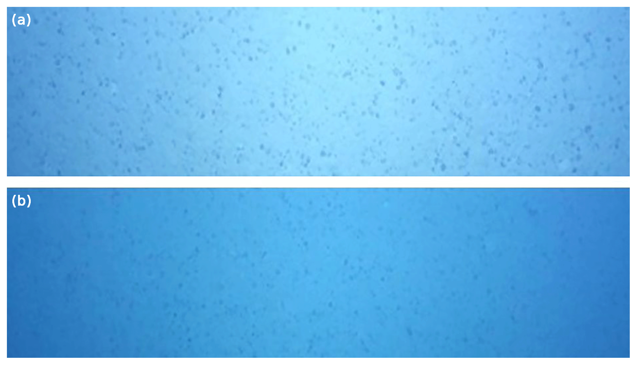
Figure 8Adjacent AUV photos from consecutive dive tracks that were obtained inside subarea b from (a) lower (5–7 m) and (b) higher (9–11 m) altitudes. Note the decrement in the image brightness. (The area of the photos represents the central part of the photo, i.e., ca. 1∕4 of the original photo size.)
Spatial distribution of median size. Plotting of the median size in square centimeters (Fig. 9) showed that the number of Mn nodules m−2 is anti-correlated to the median Mn-nodule size. The Spearman's rank correlation coefficient and R2 between these two variables are −0.50 and 0.25, respectively, supporting this observation (Fig. 10a); other studies found similar results (Okazaki and Tsune, 2013; Kuhn and Rathke, 2017; Peukert et al., 2018a). The box plot analysis of the median size values between the H–H and L–L clustered groups showed that although the L–L group contains the entire range of median size values (2.8 to 15.9 cm2), the H–H group does not contain values above 10 cm2 (2.7–10 cm2). This means in consequence that in areas with significant clustering of higher numbers of Mn nodules m2, the size of Mn nodules tends to be smaller (Fig. 10b).
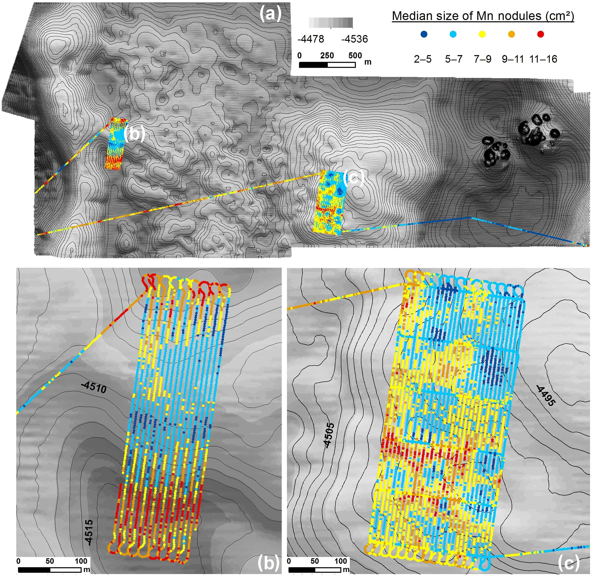
Figure 9(a) The spatial distribution of median Mn-nodule size (in cm2). (b) The estimation of median Mn-nodule size in subarea b and mainly in its southern part has been probably affected by the nonconstant altitude of the AUV. (c) The distribution of the median size inside subarea c shows also a clumped pattern.
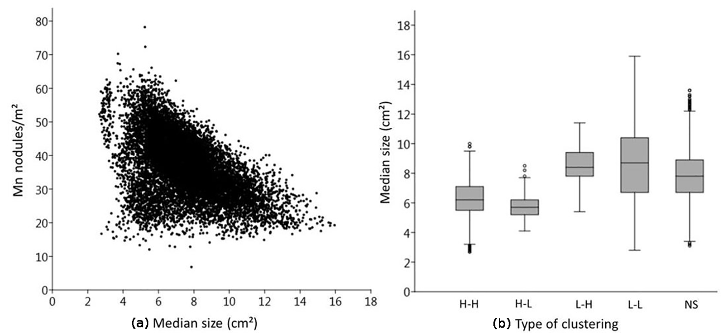
Figure 10(a) The plot of median size (cm2) and number of Mn nodules m−2. (b) The range of median size (cm2) in each type of cluster. Note the distinct difference in the range between the H–H and L–L cluster type.
4.3 RF predictive modeling
4.3.1 Effect of training sample size and ntree and mtry parameters
The results of the modeling procedure demonstrate that the RF algorithm is influenced by the size of the training sample (Fig. 11a). This finding is in accordance with other studies, in which larger training samples tended to increase the performance of RF (Li et al., 2010, 2011b; Millard and Richardson, 2015). The inclusion of a more representative range of the observed values, and consequently a larger spectrum of the causal underlying relationships, assists the RF to build a better model for the prediction of the value distribution inside the study area. For our data, the decrement becomes smaller when the size of the training sample increases further; it reaches a minimum value of 0.2 between 80 % and 90 %, showing that these additional 10 % do not notably benefit the RF model. However, the absence of stabilization of the error to a minimum value indicates that more optical data are needed from this block. The small decrement in error between 80 % and 90 % was the decisive factor to select 80 % of the data as training samples (also considering the larger number of remaining validation data and the reduced computational effort). Based on this data set, the examination of different numbers of trees showed that the RF error remains constant after 600 trees (Fig. 11b). Less trees result in a larger error; this becomes particularly evident with less than 300 trees. With more than 300 trees the range of the error is reduced (Appendix B). A higher number of trees enables higher mtry values as there are more opportunities for each variable to occur in several trees (Strobl et al., 2009). Similarly to the ntree parameter, a larger number of mtry values results in a reduced error (Fig. 11c). The error reaches a minimum and cannot be reduced further for mtry = 6; with values below 3, the error increases significantly. The different numbers of ntree reduced the error by only 0.6 in the MSR (from 18.8 to 18.2); in contrast, different mtry values reduced the error by 5.8 in the MSR (23.4 to 17.6), highlighting its importance for the prediction accuracy. In general a higher number of mtry values is suggested for RF studies with correlated variables to result in a less biased result regarding the importance of each variable; this is because the higher number increases the competition between highly correlated variables, giving more chances for different selections (Strobl et al., 2008). The finally selected mtry value of 6 coincides with the recommended approach for mtry (default, half of the default, and twice the default) suggested by Breiman (2001a). Despite the importance of this analysis, within the model with 80 % of the data as a training sample, the decrease in error by the use of RF tuned values instead of RF default values was only 0.7 in the MSR values, whilst the greatest reduction in error (16.5 in the MSR values) came from the increase in training data set size. This highlights the increased sensitivity of the method with respect to training data and that the recommended settings in the R randomForest package (Lia and Wiener, 2002) give trustworthy results, increasing its simplicity and operational character.
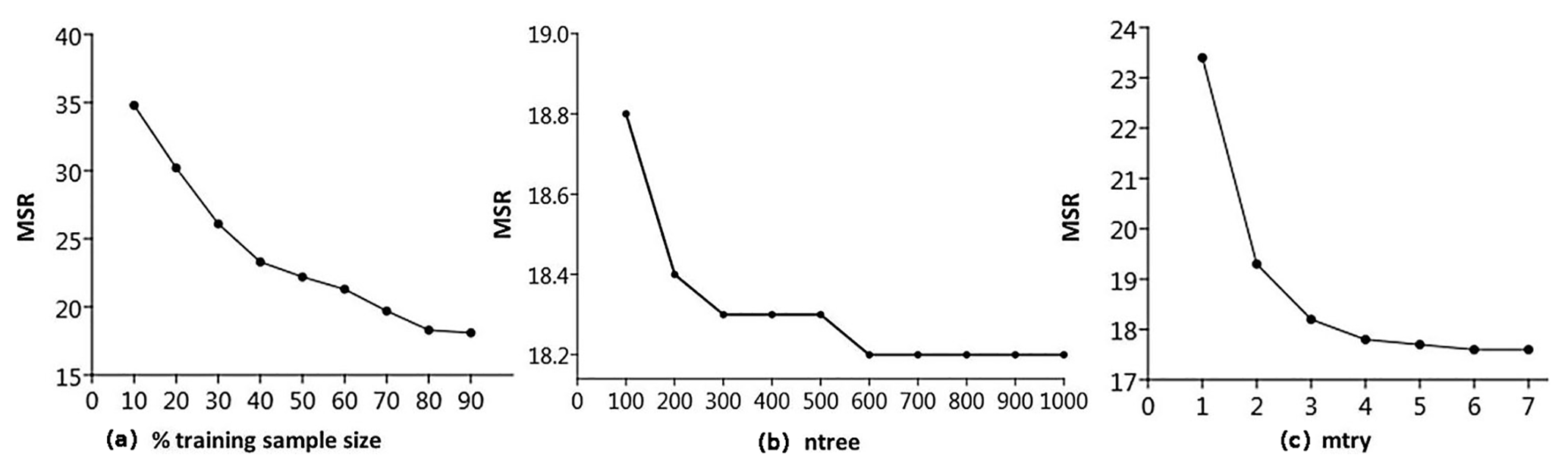
Figure 11(a) The effect of training sample size in RF error (in MSR). (b) The effect of the ntree parameter in RF error (in MSR) for the 80 % training size. (c) The effect of the mtry parameter in RF error (in MSR) for the 80 % training size.
4.3.2 Selection, application and external validation of the optimal model
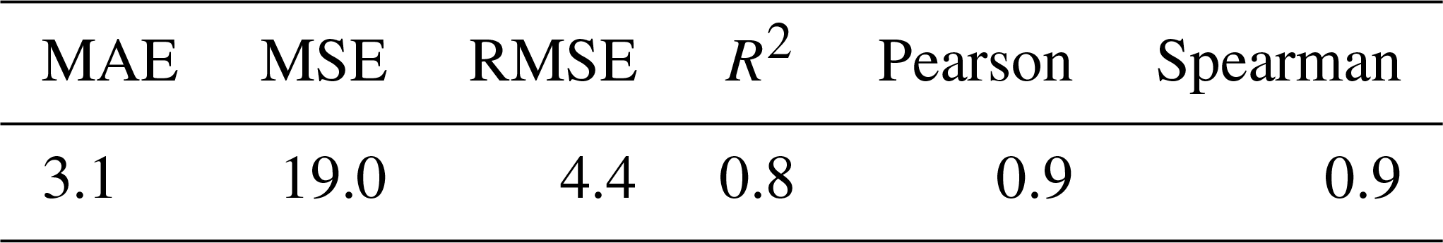
Based on the abovementioned findings, the optimal RF regression model, which uses 80 % of training data, 600 trees, and 6 predictor variables to be randomly selected at each node, was selected and applied to the entire block G77. The comparison of the predicted values with the observed values from the remaining 20 % (2255 observations) of validation data showed a good predictive performance (Table 4). Analytically, MAE and RMSE have very low values, R2 has a high value, and both Pearson's and Spearman's correlation coefficients show a strong positive correlation between the predicted and observed values. The small deviation between MAE and RMSE and the same good correlation of the Pearson and Spearman factor point towards the absence of extremely high or low predicted values (outliers). Moreover, the performance is rather stable among all the iterations (Appendix B).
Table 4The values of validation measures between predicted and observed data.
The scatterplot and box plot (Fig. 12a and b) illustrate this good match between predicted and observed values, as confirmed also by the descriptive statistics (Table 5). The residual analysis confirmed further the robustness of the model (Appendix B).
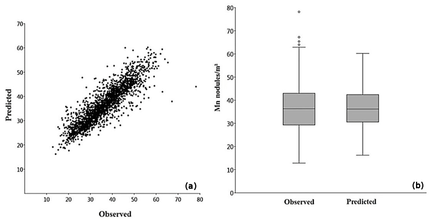
Figure 12Comparison between observed and predicted values: scatterplot (a) and box plots (b).
Table 5Descriptive statistics of observed and predicted values.
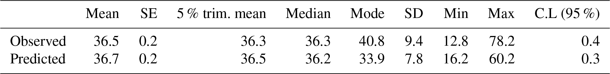
The statistical analysis also reveals the limitations of the RF model which cannot predict beyond the range of training values. It underestimates the maximum predicted values and overestimates the minimum values (Fig. 12b and Table 5), a limitation also mentioned by other authors (e.g., Horning, 2010). This happens because in regression RF, the result is the average value of all the predictions (Breiman, 2001a).
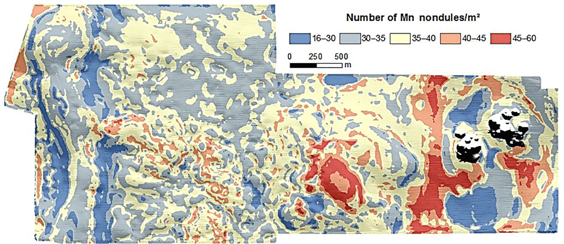
4.3.3 RF-predicted distribution of Mn nodules m−2
The final application of the RF model for the entire block G77 predicts that the majority of the area is covered by 30–45 Mn nodules m−2 (Fig. 13). In the central western part the distribution is quite uniform (at this scale) with few small areas of lower numbers. In the western part, there are two extended areas along the base of the hill with the lowest number of Mn nodules m−2. Both of these areas have a linear shape in N–S direction and follow the seafloor topography with increased slope (> 3∘). The third main patch with minimum Mn nodules m−2 occurs in the eastern depression part. In contrast, areas with a higher number of Mn nodules m−2 are located mainly in the central upper part of the hill and eastward facing slope of eastern depression and south of the subrecent hydrothermally active area.
4.3.4 RF importance
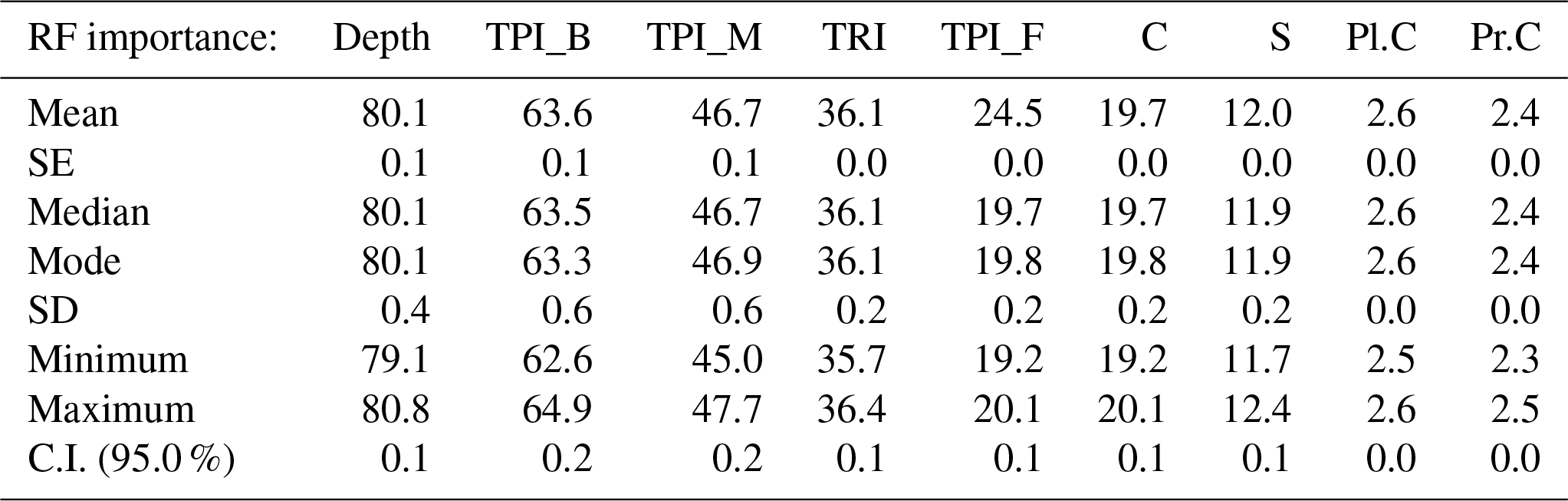
The analysis of the RF variable importance showed that the best explanatory variable for the distribution of Mn nodules m−2 is depth (Fig. 14a). The partial dependence plot of depth shows that there are specific depths, which promote higher numbers of Mn nodules m−2 aggregated in a nonlinear way (Fig. 14b). The two most important variables are the TPI_B and TPI_M. TRI, TPI_F, C, and S follow in importance (Fig. 14a). All of them also contribute in a nonlinear way. (Appendix B). Pl.C and Pr.C do not contribute significantly as explanatory variables in the performance of the RF model (Fig. 14a and Appendix B). Although the RF demonstrates good overall performance, the small study area and the arbitrary choice of the spatial scales for the TPI and other derivatives limit the potential of these variables as indicative explanatory variables on a broader scale. It is well established that surface derivatives are scale-dependent with different analysis scales to create alterations in results. Thus the combined use of different scales (here TPI) in the analysis and modeling procedure can produce models that do capture the natural variability and scale dependence (Wilson et al., 2007; Miller et al., 2014; Ismail et al., 2015; Leempoe et al., 2015). Due to the lack of relevant literature for AUV scale data sets, the C and TRI were created with the default scales of SAGA GIS v.6.3.0, while the three different TPI values were selected based on the minimum possible correlation among them.
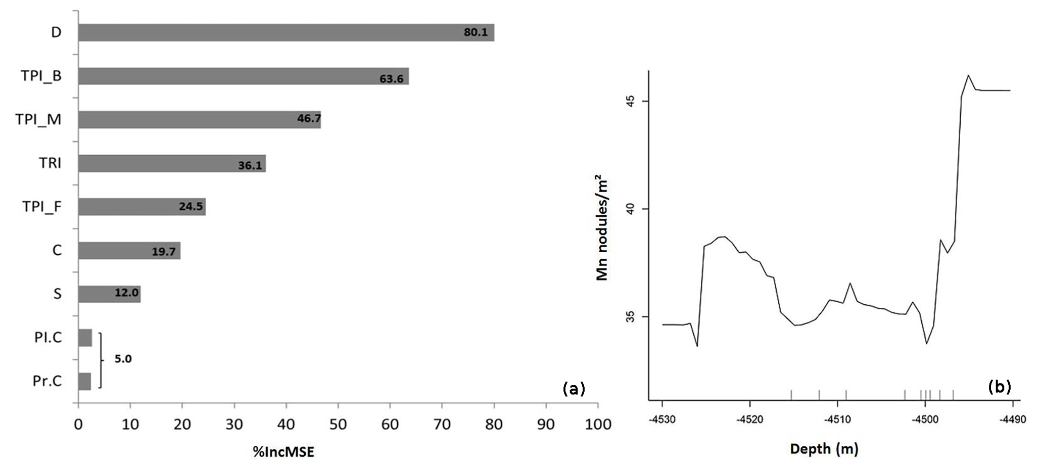
Figure 14(a) The variable importance of each predictor in the RF model. (b) The partial dependence plot of depth. The ticks on the graphs indicate the deciles of the data.
4.3.5 Estimation of abundance (kg m−2) of Mn nodules
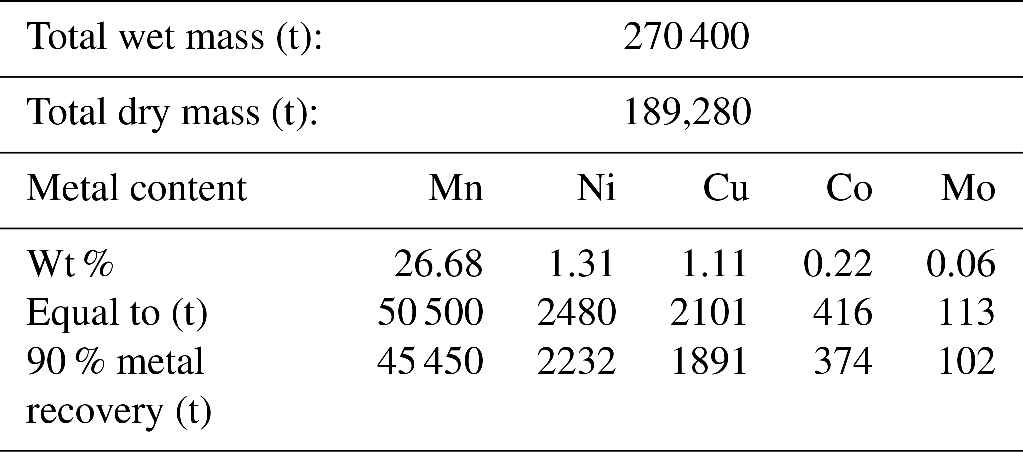
The predicted Mn-nodule distribution was combined with the abundance from box corer data (and corrected with the ratio of buried to unburied Mn nodules, in order to include the top ∼15 cm of the sediment), resulting in the Mn nodules' abundance map shown in Fig. 15. According to this map, block G77 is a promising area for mining operations. The entire block is above the cutoff abundance of 5 kg m−2 (UNOET, 1987), with a mean value of 33.8 kg m−2. We calculated that 84 % of block G77 has slopes below 3∘; steeper slopes are located mainly at the outer parts of the block, a fact that would ease establishing an ideal mining path. In this respect, the AUV scale mapping provides vital information for a potential mining path by decreasing the possibility of machine failure due to poorly mapped steep slopes not detected by, e.g., ship-based bathymetry (Peukert et al., 2018b). Mn-nodule distribution maps with this resolution increase the mining efficiency because local deposit variations can significantly affect the performance of the pickup rate, which is likely determined by technical parameters of the mining vehicle as well as the size, burial depth, and abundance of Mn nodules in the seafloor (Chung, 1996). The exclusion of areas with slopes > 3∘ resulted in 8 km2 minable seafloor surface. Assuming a constant 80 % collection efficiency (Volkmann and Lehnen, 2018) and a 30 % reduction in the Mn-nodule weight by the removal of water (Das and Anand, 2017), the dry mass of Mn nodules that can be extracted from the surface and the first 15 cm of the sediment column amounts to ca. 190 000 t. In a back-of-the-envelope calculation this quantity – assuming constant metal content inside the study area, equal to the average metal concentrations inside the CCZ (Table 6) (Volkmann, 2015), and 90 % metal recovery efficiency – could result in an estimated resource haul of 45 450 t Mn, 2232 t Ni, 1891 t Cu, 374 t Co, and 102 t Mo (Table 6).
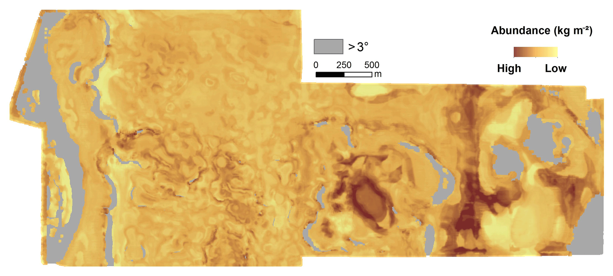
Figure 15The total abundance of Mn nodules from the surface and embedded in the sediment (max 15 cm), in areas with slope ≤3∘ inside block G77 (continuous values of abundance are not given due to confidentiality).
Table 6The estimated amount of metal mass for five metals, based on the average values of metal content inside CCZ and a five-metal HCL-leach recovery method (Volkmann, 2015).
We present a case study that highlights the applicability of the combination of AUV bathymetric and optical data for Mn-nodule resource modeling using RF machine learning. The use of AUVs for collecting hydroacoustic and optical data in areas of scientific and commercial interest can provide more precise bathymetric and Mn-nodule distribution maps. Regarding the bathymetric maps, the accurate and detailed reconstruction of the seafloor bathymetry at meter-scale resolution enables to use bathymetry and its derivatives as source data layers within a high-resolution RF model. These data should have high-quality characteristics, as the presence of acquisition artefacts may affect the robustness of the modeling procedure (Preston, 2009; Herkül et al., 2017). The combined use of cameras as the DeepSurveyCamera (Kwasnitschka et al., 2016) for acquiring high-resolution photographs and an automated analysis with a state-of-the-art algorithm (Schoening et al., 2017a) provide essential quantitative information about the distribution of Mn nodules. Image analysis results are more robust for constant AUV altitudes (7–9 m) above flat areas (< 3∘), while the alternation of the flying altitude and camera orientation during the ascending and descending phases limits the quality of the obtained images and can affect the derived number of Mn nodules m−2 .
Inside block G77, the number of Mn nodules m−2 seems to follow a normal distribution without extreme outliers and without being linearly correlated with the predictor variables used. Spatially, a clumped autocorrelated pattern is demonstrated, mainly with clustered areas of H–H and L–L values. It is still unclear if this heterogeneity is caused by external processes (e.g., topographic characteristics, geochemical conditions, or the availability of nucleus material) or if it results from the interaction of neighboring Mn nodules. The areas with a higher number of Mn nodules could provide more fragments as potential nucleus material. However, the less available space in these areas may make individual Mn-nodule growth more difficult, resulting in smaller median sizes. Conversely, a recent study from Kuhn and Rathke (2017) showed that the blanketing of the Mn nodules by sediments is higher for larger Mn nodules and, as a result, fewer large nodules will be counted, resulting in biased results in areas where the Mn nodules are bigger. Probably all of these effects can happen at the same time (with different degrees of influence), promoting a given, scale-dependent spatial structure.
This study did not consider the geochemical properties of the sediments as input data in the modeling process, which might give additional clues as to why Mn nodules are distributed as they are. However, RF importance and partial dependence plots show that bathymetric and topographic factors tend to affect this distribution in a nonlinear way and with the bulk of data plotting in specific ranges of the bathymetric derivatives. Classic studies have shown that the bathymetry and the variation in the topographic characteristics of the seafloor affects the sediment deposition environment and bottom currents and thus also geochemical processes in the sediment. All these factors determine Mn-nodule growth and thus affect the distribution of Mn nodules on regional scales (e.g., Craig, 1979; Sharma and Kodagali, 1993). It is still unknown how these properties influence the Mn-nodule distribution on meter to tens of meter scales as seen in our AUV data. The nonlinear relationship between Mn nodules and bathymetry on such high-resolution scales only began to be investigated very recently (e.g., Peukert et al., 2018; Alevizos et al., 2018). To elaborate more on the hydrodynamic and geochemical reasons behind the observed distribution pattern, we would need more investigations at and in the sediment on the same scale.
It should be acknowledged that the aim of any ML predictive model is to derive accurate predictions based on an existing (large) number of measurements to capture a complex underlying relationship (e.g., nonlinear and multivariate) between different types of data, for which our theoretical knowledge or conceptual understanding is still under development (Schmueli, 2010; Lary et al., 2016). Especially due to the constantly increasing size of scientific multivariate data in marine sciences and the existence of such nonlinear relationships between predictor and response variables (e.g., Zhi et al., 2014; Li et al., 2017), ML and RF are considered important analytic tools that can objectively reveal patterns of a (unknown) phenomenon (Genuer et al., 2017; Kavenski et al., 2009; Lary et al., 2016). Such predictions may be used to derive causalities or may drive the creation of new hypotheses. In other words, for a predictive model, the “unguided” data analyses come first and the interpretation follows (Breiman, 2001b; Schmueli, 2010; Obermeyer and Emanuel, 2016). This “a priori” knowledge of the distribution of the Mn-nodule number and size on such a scale can contribute to the biological data survey planning, too. Recent studies showed that the abundance and species richness of nodule fauna inside the CCZ is affected by the abundance of Mn nodules (Amon et al., 2016; Vanreusel et al., 2016) as well as their size (Veillette et al., 2007). Thus, high-priority areas (e.g., those with the highest commercial interest) can be targeted for sampling based on the results of optic data and RF modeling. The RF modeling takes advantage of the multilayer information (here: hydroacoustic and optical data), handling their complex relationships effectively while being resistant to overfitting (Breiman, 2001a). Moreover, the randomization of the input training points in each tree in each run results in a completely different training data set each time with mixed points from the entire study area. This random selection and mixing of points is appropriate for clustered data, as it ignores their spatial locations and consequently limits the influence of spatial autocorrelation (Appendix B). Along these lines, several authors have included the values of latitude/longitude and even the LMI values as predictor variables in order to increase the model performance (e.g., Li, 2013; Li et al., 2011b, 2013). RF has a high operational character due to its relatively simple calibration, which does not request extensive data preparation/transformation or the need for geostatistical assumptions (e.g., stationarity). The selection of the MGET toolbox (Roberts et al., 2010) further increased the simplicity of the workflow, as the RF modeling was performed entirely inside a graphic environment familiar to many geoscientists. As RF model runs can be implemented inside various software packages in future implementations of this workflow, it would be interesting to include the uncertainty for the associated predictions, e.g., with the use of the quantile regression forests (Meinshausen, 2006) from the quantregForest R package (Meinshausen, 2012). However, this will increase the computational time (Tung et al., 2014) and the simplicity of the procedure, especially if other recently proposed methodologies of estimating the uncertainty are used: the jackknife method (Wager et al., 2014), the Monte Carlo approach (Coulston et al., 2016), and the U statistics approach (Mentch and Hooker, 2016).
Similarly to other studies (e.g., Cutler et al., 2007; Millard and Richardson, 2015), RF showed increased stability in its performance, allowing a small number of iterations to compute sufficient results. The examination of the main two tuning parameters (ntree and mtry) showed that the model performance can be increased compared to default values. However, the largest improvement results from using more training data. In this respect, more photos would potentially improve the RF performance as no clear threshold was observed. Although the number of 11 276 photos seems to represent a large data set, the heterogeneity of the distribution and the occurrence of spatial clusters (patches) in different sizes and the inherent need of RF and ML in general for big training data sets (van der Ploeg et al., 2014; Obermeyer and Emanuel, 2016) stresses the need for collecting more and well-distributed data. The influence of the number of training data for model performance still remains a discussion point between studies showing an improvement by adding more data (e.g., Bishop, 2006) and other studies presenting stable performance of the model even if more data are added (e.g., Zhu et al., 2012). The availability of more data, especially if they are better distributed (i.e., data that will include the entire range of the number of Mn nodules m−2 and come from all the different sub-terrains), would most likely reinforce the model to build better and wider relationships between the predictor and response variables, keeping also a larger number of validation data points.
Finally, the resource assessment showed that block G77 is a potential mining area with high average Mn-nodule density and gentle slopes. While the threshold of 3∘ (UNOET, 1987) was used here, newer plans for mining machines seem to enable operations on steeper slopes (Atmanand and Ramadass, 2017), increasing the total amount of collected Mn nodules within the area considered herein.
The results of this study show that the acquisition and analysis of optical seafloor data can provide quantitative information on the distribution of Mn nodules. This information can be combined with AUV-based MBES data using RF machine learning to compute predictions of Mn-nodule occurrence on small operational scales. Linking such spatial predictions with sampling-based physical Mn-nodule data provides an efficient and effective tool for mapping Mn-nodule abundance.
The data used in this work are available at PANGAEA. This includes MBES ship-based data (Greinert, 2016), optical imagery (Greinert et al., 2017; Schoening, 2017c), and the source code of the CoMoNoD algorithm (Schoening, 2017b). The MBES AUV-based data are not publicly available due to the confidentiality of coordinates.
A1 Hydroacoustic data acquisition and post-processing
The calculation of the bathymetric derivatives was performed with the SAGA GIS v6.3.0 Morphometry library (http://www.saga-gis.org/saga_tool_doc/6.3.0/ta_morphometry.html, last access: 6 December 2018).
A2 Spatial statistics
Global Moran's I and local Moran's I were performed with the ArcMap™ 10.1 software, using the Spatial Statistics toolbox, according to the equations provided. As a null hypothesis, it is assumed that the examined attribute is randomly distributed among the features in the study area. For the optimal conceptualization of spatial relationships, the inverse Euclidian distance method was selected, as it is appropriate for modeling processes with continuous data in which the closer two samples are in space, the more likely they are to interact/influence each other or have been influenced for the same reasons. The distance threshold was set at 50 m, and the increment analysis was performed with a step of 50 m. Moreover, the spatial weights were standardized in order to minimize any bias that exists due to sampling design (uneven number of neighbors). Apart from the index value, the p value and Z score are also provided. The local Moran's I indicates statistically significant clusters and outliers for a 95 % confidence level. The high number of observations (≫30) that was used ensures the robustness of the indexes.
Table A1Spearman's correlation coefficient for each pair of predictor variables.

A3 RF predictive modeling (selection of predictor variables)
Correlation among the derivatives was checked by the Spearman's correlation coefficient (ρ). This coefficient was preferred due to the skewed distribution of the values in the derivatives. The majority of the possible pairs is uncorrelated or weakly correlated. Only C vs. TPI_F and TRI vs. S have a strong correlation. However, they should not be excluded as they express different topographic characteristics and they are not correlated with the remainder of derivatives. It should be mentioned that in similar studies even higher thresholds have been used during the selection of predictor variables (Che Hasan et al., 2014; Li et al., 2016, 2017).
The nine training samples with different sizes were created by the MGET tool “Randomly Split Table into Training and Testing Records”. The spatial randomness of the procedure, combined with the many available data, resulted in training samples with similar descriptive statistics.
B1 RF predictive modeling (calibration of the model)
The descriptive statistics of the performance of each model were used as decision factors for the number of iterations (Tables B1–B5). In all cases, the mean value with very low standard error, very low standard deviation, range, and the 95 % confidence interval indicate a rather stable performance, without the need for further iterations.
Table B1Descriptive statistics of MSR from different training set sizes, after 10 iterations with default settings.
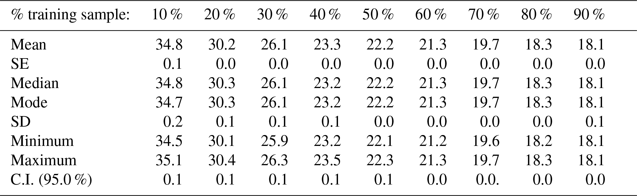
Table B2Descriptive statistics of MSR from a different number of the ntree parameter, after 10 iterations with 80 % of the sample as training data and mtry = 3.
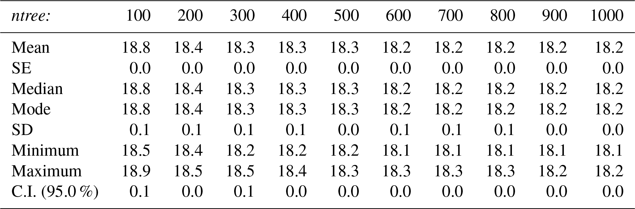
Table B3Descriptive statistics of MSR from different number of the mtry parameter, after 10 iterations with 80 % of the sample as training data and ntree = 600.
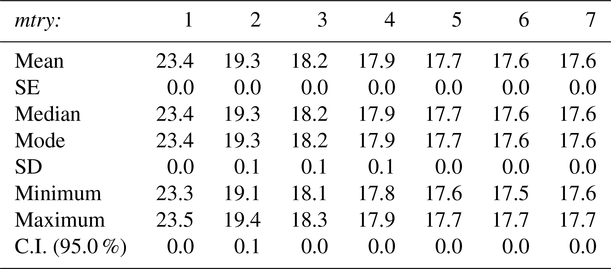
Table B4Descriptive statistics of MSR for the optimum selected RF model, after 30 iterations with 80 % of the sample as training data, ntree = 600, and mtry = 6.

Table B5Descriptive statistics of RF importance for the optimum RF model, after 30 iterations with 80 % of the sample as training data, ntree = 600, and mtry = 6.
B1.1 Data exploration
The histogram of Mn nodules m−2 (Fig. B1) shows a good fit with the superimposed theoretical normal curve, with the shape of the distribution being rather symmetrical. This fact is supported by the equal 5 % trimmed mean and median and the slightly different mode (Table B6). Similarly, the visual inspection of the probability plot (Fig. B1) shows a good match as a linear pattern is observed for the greatest part, with slight deviation existing only in the outer parts of the curve. According to the box plot, there are only 21 mild outliers (according to Hoaglin et al., 1986; Dawson, 2011), which correspond to 0.18 % of the total observation. This percentage is smaller than the 0.8 % threshold that has been suggested for normal disturbed data (Dawson, 2011).The small values for skewness and kurtosis combined with the large sample size further support the normally distributed pattern of the data (Table B6). Especially for large data samples, measurements of skewness and kurtosis combined with the visual inspection of histogram and probability plot are recommended ways of examining the normality (D'Agostino et al., 1990; Yaziki and Yolacan, 2007; Field, 2009; Ghasemi and Zahediasl, 2012; Kim, 2013).
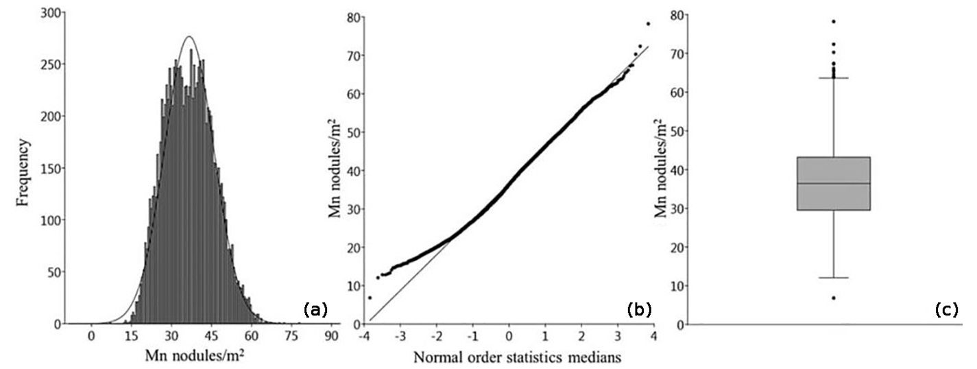
Figure B1(a) Histogram of Mn nodules m−2 with the superimposed normal curve. (b) The normal probability plot of Mn nodules m−2. (c) The box plot of Mn nodules m−2.
Table B6The descriptive statistics of the number of Mn nodules m−2.

The potential linear correlation between depth, bathymetric derivatives, and the number of Mn nodules m−2 was investigated using the Spearman's rank correlation coefficient (ρ) (Table B7) because of the skewed distribution and presence of extreme values in the depth and bathymetric derivative values (Mukaka, 2012).
Table B7The Spearman's rank correlation coefficient between Mn nodules m−2, depth, and bathymetric derivatives.

B1.2 Selection, application, and external validation of the optimal model
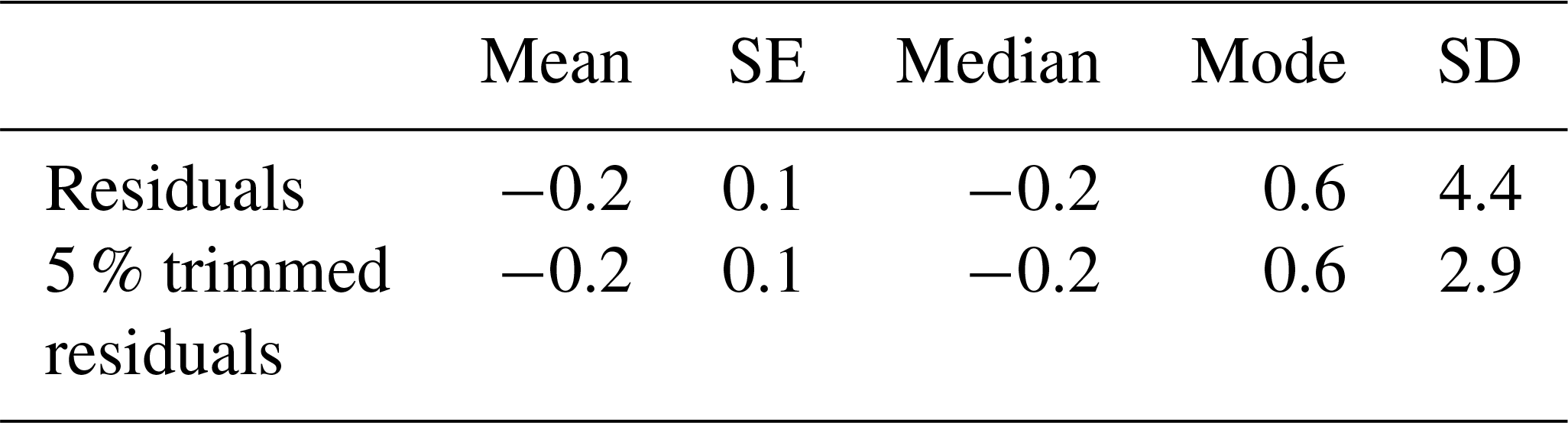
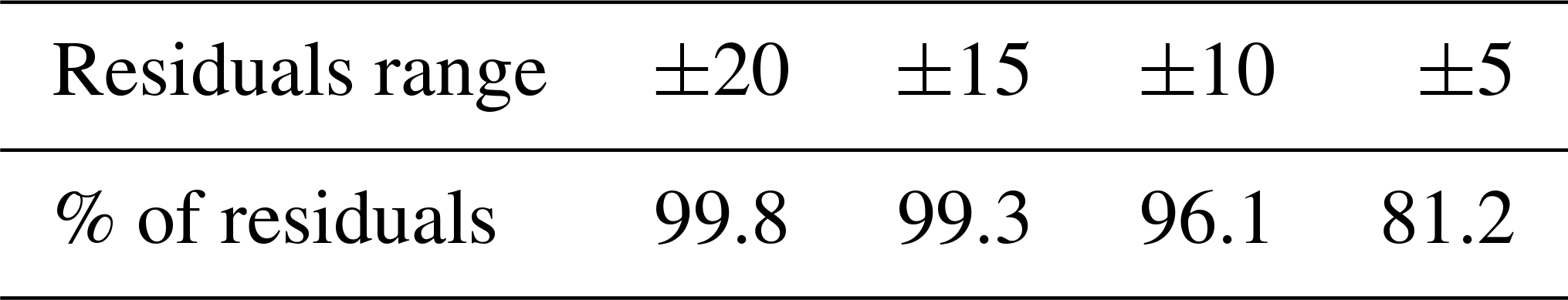
Despite the fact that RF is a full nonparametric technique and there is no need for the residuals to follow specific assumptions (Breiman, 2001a), the examination of them can provide an in-depth look at RF performance characteristics. The scatterplot of residuals against predicted values shows a random pattern, which is also confirmed by the low values of Pearson, Spearman, and R2 coefficients between predicted values and residuals (Fig. B2 and Table B8). Moreover, the residuals tend to cluster towards the middle of the plot without being systematically high or low and having a zero mean value (Fig. B2 and Table B9). Their constant variance (homoscedasticity) implies that the distribution of error has the same range for almost all fitted values. Indeed, 99.3 % of the residuals are inside the range ±15 and 81.2 % are inside the range ±5 (Table B10). The presence of outliers is very limited without affecting the main statistical characteristics of residuals (Table B9), indicating that the model adequately fits the overwhelming majority of the observations (> 2165) and only random variation (that exists in any real, natural phenomenon) or noise can occur.
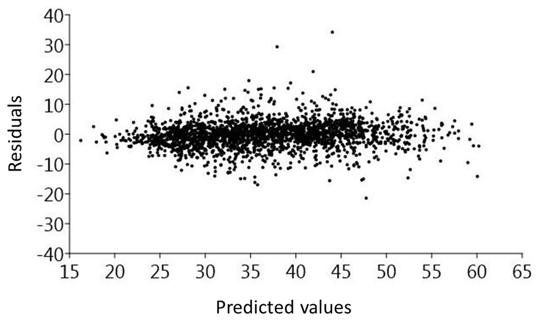
Table B8Pearson, Spearman, and R2 correlation coefficients between residuals and predicted values.

Table B9Main descriptive statistics of residuals and 5 % trimmed residuals.
The spatial autocorrelation analysis of the residuals using the global Moran's index (same settings as Appendix A), showed low spatial autocorrelation (I=0.112112, p<0.01 and Z score > 2.58). The index number of the residuals is relatively low compared with the high initial values of the original data (I=0.69890 and I=0.697747 for the entire data set and the 80 % training data set, respectively). Moreover, the spatial autocorrelation of the 5 % trimmed residuals is only 0.093832. According to similar studies (i.e., regression RF), the presence of spatial autocorrelation in the residuals of the model can result in underestimation of the true prediction error (Ruß und Kruse, 2010). The presence of low spatial autocorrelation values in the residuals of regression RF has been reported also by other authors (e.g., Mascaro et al., 2014; Xu et al., 2016), and it is a common problem in all the well-established machine learning methods (e.g., random forests, neural network, gradient boosting machines, and support vector machines) when dealing with regression predictions of spatial variables (Gilardi and Bengio, 2009; Ruß und Kruse, 2010; Santibanez et al., 2015a, b). The spatial plotting and visual examination of the residuals (Fig. B3) showed that this spatial clustering exists mainly in the small subarea b and especially in the areas which are associated with an increased slope (>3∘), where the AUV is forced to vary its altitude between the ascending and descending phase and consequently affects the image quality and the later modeling results.
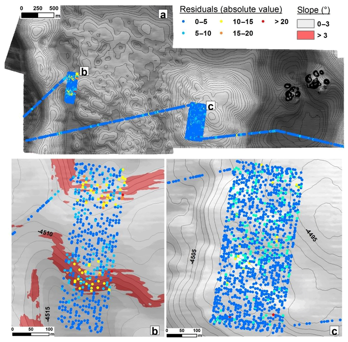
Figure B3Spatial plotting of the RF residuals (absolute values). The intervals of their range are in accordance with the Table B10.
B1.3 RF importance
The production of the RF partial dependence plots show the nonlinear character between the Mn nodules m−2 and the bathymetric derivatives.
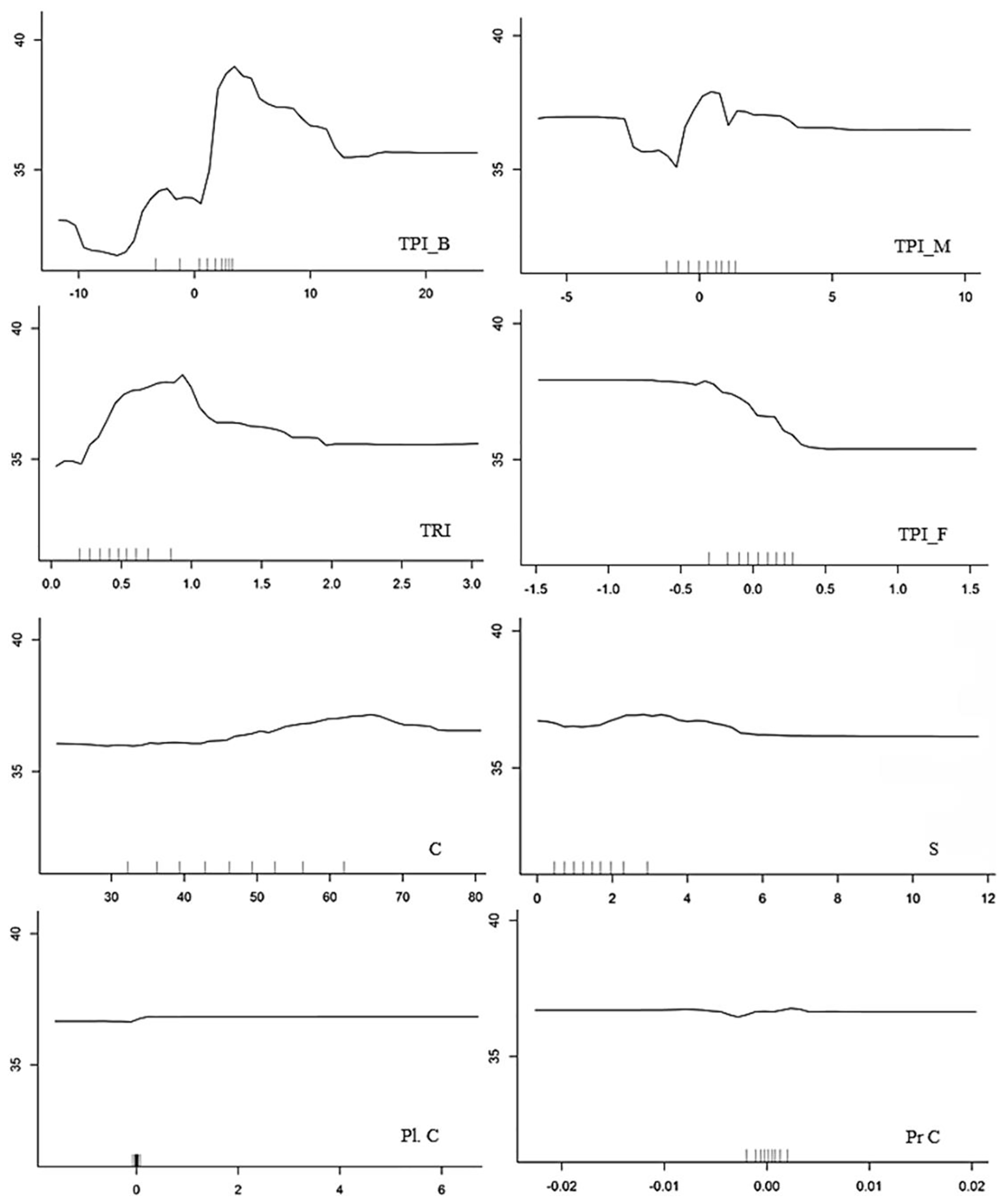
Figure B4Partial dependence plots for each of the predictor variables. The y axis represents the number of Mn nodules m−2 and the x axis the values of each predictor variable (depth derivatives). The ticks on the graphs indicate the deciles of the data.
IZG processed the MBES and AUV data, performed the RF modeling, the statistical and GIS analysis, and wrote the paper. TS contributed to the survey design with respect to the optic data, developed the CoMoNoD algorithm, and processed the optic data. EA was involved in developing the idea of using RF for modeling and contributed to the GIS analysis. JG contributed to the survey by designing the MBES and the optic data survey planning, acquiring the MBES and the optic data, verifying the analytical methods, and supervising the project. All authors discussed the results, provided critical feedback, and contributed to the final paper.
The authors declare that they have no conflict of interest.
This article is part of the special issue “Assessing environmental impacts of deep-sea mining – revisiting decade-old benthic disturbances in Pacific nodule areas”. It is not associated with a conference.
We thank the captain and crew of RV Sonne for their contribution to
a successful cruise. We express our gratefulness to the GEOMAR AUV team for
their support during the cruise. We thank Anja Steinführer for
preprocessing of the AUV MBES data and Mareike Kampmeier for advice during
the post-processing analysis of the MBES data. We thank Inken Preuss for
proofreading the paper. Finally, we thank the GEOMAR Library team for its
support in gathering the necessary bibliography. All data were acquired
within the framework of the JPIO Project “Ecological Aspects of Deep-Sea
Mining”, funded through BMBF grant 03F0707A. Funding for Iason-Zois Gazis
was also made available through MarTERA grant COMPASS-Drimp from BMWi
(03SX466B). This is publication 35 of the DeepSea Monitoring Group at GEOMAR
Helmholtz Centre for Ocean Research Kiel.
Edited by: Daniel O. B. Jones
Reviewed by: two anonymous
referees
Alevizos, E., Schoening, T., Koeser, K., Snellen, M., and Greinert, J.: Quantification of the fine-scale distribution of Mn-nodules: insights from AUV multi-beam and optical imagery data fusion, Biogeosciences Discuss., https://doi.org/10.5194/bg-2018-60, in review, 2018.
Anselin, L.: Local Indicators of Spatial Association – LISA, Geogr. Anal., 27, 93–115, https://doi.org/10.1111/j.1538-4632.1995.tb00338.x, 1995.
Atmanand, M. A. and Ramadass, G. A.: Concepts of Deep-Sea Mining Technologies, in: Deep-Sea Mining, edited by: Sharma, R., Resource Springer, Cham. Online ISBN 978-3-319-52557-0, https://doi.org/10.1007/978-3-319-52557-0_6, 2017.
Bellingham, J.: Autonomous underwater vehicles (AUVs), in: Encyclopedia of Ocean Sciences, edited by: Steele, H., Academic Press, San Diego, 212–216, https://doi.org/10.1006/rwos.2001.0303, 2001.
Bingham, D., Drake, T., Hill, A., and Lott, R.: The Application of Autonomous Underwater Vehicle (AUV) Technology in the Oil Industry – Vision and Experiences. FIG XXII International Congress Washington, DC USA, 19–26 April, 1–13, 2002.
Breiman, L.: Random forests, Machine Learning, 45, 5–32, https://doi.org/10.1023/A:101093340, 2001a.
Breiman, L.: Statistical Modeling: The Two Cultures, Stat. Sci., 16, 199–215, https://doi.org/10.1214/ss/1009213726, 2001b.
Caress, D. W. and Chayes, D. N.: MB-System: Mapping the Seafloor, available at: https://www.mbari.org/products/research-software/mb-system (last access: 6 December 2018), 2017.
Caress, D. W., Thomas, H., Kirkwood, W. J., McEwen, R., Henthorn, R., Clague, D. A., Paull, C. K., and Paduan, J.: High-resolution multibeam, sidescan and subbottom surveys using the MBARI AUV D, in: Marine Habitat Mapping Technology for Alaska, edited by: Allan, B.,Greene, H. G., and Reynolds, J. R., Alaska Sea Grant College Program, University of Alaska Fairbanks, 47–69, https://doi.org/10.4027/mhmta.2008.04, 2008.
Carranza, E. J. M. and Laborte, A. G.: Random Forest Predictive Modelling of Mineral Prospectivity with Small Number of Prospects and Data with Missing Values in Abra (Philippines),Comput. Geosci., 74, 60–70, https://doi.org/10.1016/j.cageo.2014.10.004, 2015a.
Carranza, E. J. M. and Laborte, A. G.: Data-driven predictive mapping of gold prospectivity, Baguio district, Philippines: Application of Random Forests algorithm, Ore Geol. Rev., 7, 777–787, https://doi.org/10.1016/j.oregeorev.2014.08.010, 2015b.
Carranza, E. J. M. and Laborte, A. G.: Data-Driven Predictive Modeling of Mineral Prospectivity Using Random Forests: A Case Study in Catanduanes Island (Philippines), Nat. Resour. Res., 25, 35–50, https://doi.org/10.1007/s11053-015-9268-x, 2016.
Chakraborty, B. and Kodagali, V.: Characterizing Indian Ocean manganese nodule-bearing seafloor using multi-beam angular backscatter, Geo-Mar. Lett., 24, 8–13, https://doi.org/10.1007/s00367-003-0153-y, 2004.
Chance, T., Kleiner, A., and Northcutt, J.: The autonomous underwater vehicle (AUV): A cost-effective alternative to deep-towed technology, Integrated Coastal Zone Management, 2, 65–69, 2000.
Che Hasan, R., Ierodiakonou, D., and Monk, J.: Evaluation of Four Supervised Learning Methods for BenthicHabitat Mapping Using Backscatter from Multi-Beam Sonar, Remote Sens., 4, 3427–3443, https://doi.org/10.3390/rs4113427, 2012.
Che Hasan, R., Ierodiaconou, D., Laurenson, L., and Schimel, A.: Integrating Multibeam Backscatter Angular Response, Mosaic and Bathymetry Data for Benthic Habitat Mapping, PLoS ONE, 9, e97339, https://doi.org/10.1371/journal.pone.0097339, 2014.
Chen, L., Wang, S., McDonald-Maier K., and Hu, H.: Towards autonomous localization and mapping of AUVs: a survey, Int. J. Intell. Syst., 1, 97–120, https://doi.org/10.1108/20496421311330047, 2013.
Chung, J. S.: Deep-Ocean Mining: Technologies for Manganese Nodules and Crusts, Int. J. Offshore Polar, 6, 244–254, 1996.
Clague, D. A., Dreyer, B. M., Paduan, J. B., Martin, J. F., Caress, D. W., Gill, J. B., Kelley D. S., Thomas, H., Portner, R. A., Delaney, J. R., Guilderson, T. P., and McGann, M. L.: Eruptive and tectonic history of the Endeavour Segment, Juan de Fuca Ridge, based on AUV mapping data and lava flow ages, Geochem. Geophy. Geosys., 15, 3364–3391, https://doi.org/10.1002/2014GC005415, 2014.
Clague, D. A., Caress, D. W., Dreyer, B. M., Lundsten, L., Paduan, J. B., Portner, R. A., Spelz-Madero, R., Bowles, J. A., Castillo, P. R., Guardado-France, R., Le Saout, M., Martin, J. F., Santa Rosa-del Rio, M. A., and Zierenberg, R. A.: Geology of the Alarcon Rise, southern Gulf of California, Geochem. Geophy. Geosy., 19, 807–837, https://doi.org/10.1002/2017GC007348, 2018.
Clements, A. J., Strong, J. A., Flanagan, C., and Service, M.: Objective stratification and sampling-effort allocation of ground-truthing in benthic-mapping surveys, ICES J. Mar. Sci., 67, 628–637, 2010.
Cochran, W. G.: Sampling Techniques, 3rd edn. Wiley, New York, 1977.
Conrad, O., Bechtel, B., Bock, M., Dietrich, H., Fischer, E., Gerlitz, L., Wehberg, J., Wichmann, V., and Böhner, J.: A system for Automated Geoscientific Analyses (SAGA) v. 2.1.4, Geosci. Model Dev., 8, 1991–2007, https://doi.org/10.5194/gmd-8-1991-2015, 2015.
Coulston, J. W., Blinn, C. E., Thomas, V. A., and Wynne, R. H.: Approximating prediction uncertainty for random forest regression models, Photogramm. Eng. Rem. S., 807, 189–197, 2016.
Craig, J. D.: The relationship between bathymetry and ferromanganese deposits in the north equatorial Pacific, Mar. Geol., 29, 165–186, https://doi.org/10.1016/0025-3227(79)90107-5, 1979.
Cutler, D. R., Edwards, T. C., Beard Karen, H., Cutler, A., Hess, K. T., Gibson, J. C., and Lawler, J. J.: Random forests for classification in ecology, Ecology, 88, 2783–2792, 2007.
D'Agostino, R. B., Belanger, A., and D' Agostino Jr., R. B.: A Suggestion for Using Powerful and Informative Tests of Normality, Am. Stat., 44, 316–321, https://doi.org/10.2307/2684359, 1990.
Danson, E.: The Economies of Scale: Using Autonomous Underwater Vehicles (AUVs) for Wide-Area Hydrographic Survey and Ocean Data Acquisition, FIG XXII International Congress Washington, DC, USA, 19–26 April, 2002.
Das, R. P. and Anand, S.: Metallurgical Processing of Polymetallic Ocean Nodules, in: Deep-Sea Mining, edited by: Sharma, R., Resource Springer, https://doi.org/10.1007/978-3-319-52557-0_12, 2007.
Dawson, R.: How Significant is a Boxplot Outlier?, J. Stat. Educat., 19, 1–13, https://doi.org/10.1080/10691898.2011.11889610, 2011.
De Moustier, C.: Beyond bathymetry: Mapping acoustic backscattering from the deep seafloor with Sea Beam, J. Acoust. Soc. Am., 79, 316–331, 1986.
Deschamps, A., Maurice, T., Embley, R. W., and Chadwick, W. W.: Quantitative study of the deformation at Southern Explorer Ridge using high-resolution bathymetric data, Earth Planet. Sc. Lett., 259, 1–17, https://doi.org/10.1016/j.epsl.2007.04.007, 2007.
Diaz-Uriarte, R. and de Andres, A.: Gene selection and classification of microarray data using random forest, BMC Bioinformatics, 7, https://doi.org/10.1186/1471-2105-7-3, 2006.
Diesing, M. and Stephens, D.: A multi-model ensemble approach to seabed mapping, J. Sea Res., 100, 62–69, https://doi.org/10.1016/j.seares.2014.10.013, 2015.
Diesing, M., Green, S. L., Stephens, D., Lark, R. M., Stewart, H. A., and Dove, D.: Mapping seabed sediments: Comparison of manual, geostatistical, object-based image analysis and machine learning approaches, Cont. Shelf Res., 84, 107–119, https://doi.org/10.1016/j.csr.2014.05.004, 2014.
Dikau, R.: Geomorphic landform modelling based on hierarchy theory, in: Proceedings of the 4th International Symposium on Spatial Data Handling, edited by: Brassel, K. and Kishimoto, H., Department of Geography, University of Zürich, Zürich, Switzerland, 230–239, 1990.
Durden, J. M., Schoening, T., Althaus, F., Friedman, A. Garcia, R., Glover, A. G., Greinert, J., Jacobsen, Stout, N., Jones, D. O. B., Jordt, A., Kaeli, J. W., Koser, K., Kuhnz, L. A., Lindsay, D., Morris, K. J., Nattkemper, T. W., Osterloff, J., Ruhl, H. A., Singh, H., Tran, M., and Bett, B. J.: Perspectives in visual imaging for marine biology and ecology: from acquisition to understanding, Oceanogr. Mar. Biol., 54, 1–72, https://doi.org/10.1201/9781315368597, 2016.
Field, A. P.: Discovering statistics using SPSS: (and sex and drugs and rock “n” roll), (OKS Print.) Los Angeles (i.e. Thousand Oaks), California, SAGE Publications, 2009.
Frazer, J. and Fisk, M. B.: Geological factors related to characteristics of sea-floor manganese nodule deposits, Deep-Sea Res. Pt. A, 28, 1533–1551, https://doi.org/10.1016/0198-0149(81)90096-0, 1981.
Fu, W. J., Jiang, P. K., Zhou, G. M., and Zhao, K. L.: Using Moran's I and GIS to study the spatial pattern of forest litter carbon density in a subtropical region of southeastern China, Biogeosciences, 11, 2401–2409, https://doi.org/10.5194/bg-11-2401-2014, 2014.
Garzón, M. B., Blazek, R., Neteler, M., Sánchez de Dios, R., Ollero, H. S., and Furlanello, C.: Predicting habitat suitability with machine learning models: The potential area of Pinus sylvestris L. in the Iberian Peninsula, Ecol. Model., 197, 383–393, https://doi.org/10.1016/j.ecolmodel.2006.03.015, 2006.
Genuer, R., Poggi J., Tuleau-Malot, C., and Villa-Vialaneix, N.: Random Forests for Big Data, Big Data Research, 9, 28–46, https://doi.org/10.1016/j.bdr.2017.07.003, 2017.
GEOMAR: Helmholtz-Zentrum für Ozeanforschung, Autonomous Underwater Vehicle “ABYSS”, Journal of large-scale research facilities, 2, A79, 1–5, https://doi.org/10.17815/jlsrf-2-149, 2016.
Ghasemi, A. and Zahediasl, S.: Normality Tests for Statistical Analysis: A Guide for Non-Statisticians, Int. J. Endocrinol. Metab., 10, 486–489, https://doi.org/10.5812/ijem.3505, 2012.
Gilardi, N. and Bengio, S.: Comparison of four machine learning algorithms for spatial data analysis, Conf. Signals Syst. Comput., 17, 160–167, 2009.
Glasby, G. P.: Distribution of manganese nodules and lebensspuren in underwater photographs from the Carlsberg Ridge, Indian Ocean, New Zealand, J. Geol. Geophys., 16, 1–17, https://doi.org/10.1080/00288306.1973.10425383, 1973.
Glasby, G. P.: Manganese nodules in the South Pacific: A review, New Zealand, J. Geol. Geophys., 19, 707–736, https://doi.org/10.1080/00288306.1976.10426315, 1976.
Goodchild, M. F.: Spatial autocorrelation. Concepts and Techniques in Modem Geography, 47, 1–56, 1986.
Grasmueck, M., Eberli, G. P., Viggiano, D. A., Correa, T., Rathwell, G., and Luo, J.: Autonomous underwater vehicle (AUV) mapping reveals coral mound distribution, morphology, and oceanography in deep water of the Straits of Florida, Geophys. Res. Lett., 33, L23616, https://doi.org/10.1029/2006GL027734, 2006.
Greinert, J.: Swath sonar multibeam EM122 bathymetry during SONNE cruise SO239 with links to raw data files, PANGAEA, https://doi.org/10.1594/PANGAEA.859456, 2016.
Greinert, J., Schoening, T., Köser, K., and Rothenbeck, M.: Seafloor images and raw context data along AUV tracks during SONNE cruises SO239 and SO242/1, GEOMAR – Helmholtz Centre for Ocean Research Kiel, PANGAEA, https://doi.org/10.1594/PANGAEA.882349, 2017.
Haase, K. M., Koschinsky, A., Petersen, S., Devey, C. W., German, C., Lackschewitz, K. S., Melchert, B., Seifert, R., Borowski, C., Giere, O., and Paulick, H.: M64/1, M68/1 and M78/2 Scientific Parties. Diking, young volcanism and diffuse hydrothermal activity on the southern Mid-Atlantic Ridge: the Lilliput field at 9∘33′ S, Mar. Geol., 266, 52–64, https://doi.org/10.1016/j.margeo.2009.07.012, 2009.
Hammer, Ø., Harper, D. A. T., and Ryan, P. D.: PAST: Paleontological statistics software package for education and data analysis, Palaeontol. Electron., 4, 9 pp., 2001.
Hari, V. N., Kalyan, B., Chitre, M., and Ganesan, V.: Spatial Modeling of Deep-Sea Ferromanganese Nodules With Limited Data Using Neural Networks, IEEE J. Ocean. Engin., 43, 1–18, https://doi.org/10.1109/JOE.2017.2752757, 2017.
Herkül, K., Peterson, A., and Paekivi, S.: Applying multibeam sonar and mathematical modeling for mapping seabed substrate and biota of offshore shallows, Estuarine, Coast. Shelf Sci., 192, 57–71, 2017.
Henthorn, R., Caress, D. W., Thomas, H., McEwen, R., Kirkwood, W. J., Paull, C. K., and Keaten, R.: High-resolution multibeam and subbottom surveys of submarine canyons, deep-sea fan channels, and gas seeps using the MBARI mapping AUV, Proceedings of the IEEE OCEANS Conference, 1–6, https://doi.org/10.1109/OCEANS.2006.307104, 2006.
Hoaglin, D. C., Iglewicz, B., and Tukey, J. W.: Performance of Some Resistant Rules for Outlier Labeling, J. Am. Stat. Assoc., 81, 991–999, 1986.
Horning, N.: RandomForests: An algorithm for image classification and generation of continuous fields data sets, International Conference on Geoinformatics for Spatial Infrastructure Development in Earth and Allied Sciences (GIS-IDEAS), 9–11 December, Hanoi, Vietnam, 2010.
Huang, Z., Justy, S., Scott, L. N., and Brendan, P. B.: Predictive mapping of seabed substrata using high-resolution multibeam sonar data: A case study from a shelf with complex geomorphology, Mar. Geol., 357, 37–52, 2014.
Ismail, K., Huvenne, V. A. I., and Masson, D. G.: Objective automated classification technique for marine landscape mapping in submarine canyons, Mar. Geol., 362, 17–32, 2015.
Iwahashi, J. and Pike, R. J.: Automated Classifications of Topography from DEMs by an Unsupervised Nested- Means Algorithm and a Three-Part Geometric Signature, Geomorphology, 86, 409–440, 2017.
Jakobsson, M., Gyllencreutz, R., Mayer, L. Dowdeswell, J. A. Canals, M., Todd, B. J., Dowdeswell, E. K., Hogan K. A., and Larter, R. D.: Mapping submarine glacial landforms using acoustic methods, Geol. Soc., London, Memoirs, 46, 17–40, https://doi.org/10.1144/M46.182, 2016.
Jung, H. S., Ko, Y. T., and Moon, J. W.: Characteristics of Seafloor Morphology and Ferromanganese Nodule Occurrence in the Korea Deep-sea Environmental Study (KODES) Area, NE Equatorial Pacific, Mar. Georesour. Geotec., 19, 167–180, https://doi.org/10.1080/10641190109353811, 2001.
Kavenski, M., Pozdnukhov, A., and Timonin, V.: Machine learning for spatial environmental data. Theory, applications and software, EPFL Press, 1st Edn., https://doi.org/10.1201/9781439808085, 2009.
Kim, H. Y.: Statistical notes for clinical researchers: assessing normal distribution using skewness and kurtosis, Restorative Dentistry and Endodontics, 38, 52–54, https://doi.org/10.5395/rde.2013.38.1.52, 2013.
Kleinrock, M. C: Capabilities of some systems used to Survey the Deep-Sea Floor, Chap. 2, in: Handbook of geophysical exploration at sea, edited by: Richard, G. A., 2nd Edn., Hard Minerals, CRC Press, p. 37, 1992a.
Kleinrock, M. C., Hey, R. N., and Theberger Jr., A. E.: Practical geological comparison of some seafloor survey instruments, Geophys. Res. Lett., 19, 1407–1410, https://doi.org/10.1029/92GL01390, 1992b.
Knobloch, A., Kuhn, T., Rühlemann, C., Hertwig, T., Zeissler, K. O., and Noack, S.: Predictive Mapping of the Nodule Abundance and Mineral Resource Estimation in the Clarion-Clipperton Zone Using Artificial Neural Networks and Classical Geostatistical Methods, in: Deep-Sea Mining, edited by: Sharma R., Resource Springer, https://doi.org/10.1007/978-3-319-52557-0_6, 2017.
Ko, Y., Lee, S., Kim, J., Kim, K. H., and Jung, M. S.: Relationship between Mn Nodule Abundance and Other Geological Factors in the Northeastern Pacific: Application of GIS and Probability Method, Ocean Sci. J., 41, 149–161, https://doi.org/10.1007/BF03022420, 2006.
Kodagali, V.: Influence of Regional and Local Topography on the Distribution of Polymetallic Nodules in Central Indian Ocean Basin, Geo-Mar. Lett., 8, 173–178, 1988.
Kodagali, V. and Chakraborty, B.: Multibeam Echosounder PseudoSidescan Images as a tool for Manganese Nodule Exploration, Proceedings of the Third Ocean Mining Symposium Goa, India, 8–10 November, 97–104, 1999.
Kodagali, V. N. and Sudhakar, M.: Manganese nodule distributionin different topographic domains of the Central Indian Basin, Mar. Georesour. Geotec., 11, 293–309, https://doi.org/10.1080/10641199309379925, 1993.
Kuhn, T. and Rathke, M.: Report on visual data acquisition in the field and interpretation for SMnN. Deliverable D1.31 of the EU-Project Blue Mining, BGR Hannover, 34 pp., 2017.
Kuhn, T., Wiedicke-Hombach, M., Barckhausen, U., Schwarz-Schampera, U., Rutkowski, J., and Lehmnn, S.: New Insights of Mn Nodule Exploration from the German License Area in the Pacific Manganese Nodule Belt, Toward the Sustainable Development of Marine Minerals: Geological, Technological, and Economic Aspects, 39th Underwater Mining Institute, 4–9 October, Gelendzhik, Russia, 2010.
Kuhn, T., Rühlemann, C., and Wiedicke-Hombach, M.: Development of Methods and Equipment for the Exploration of Manganese Nodules in the German License Area in the Central Equatorial Pacific, Proceedings of the ninth ISOPE Ocean Mining Symposium, Maui, Hawaii, USA, 19–24 June, 174–177, 2011.
Kuhn, T., Rühlemann C., and Knobloch, A.: Classification of manganese nodule estimates: can we reach the “measured resource” level? Resource and Environmental Assessments for Seafloor Mining Development, 45th Underwater Mining Conference, Incheon, Korea, 9–13 October 2016.
Kwasnitschka, T., Köser, K., Sticklus, J., Rothenbeck, M., Weiß, T., Wenzlaff, Em. , Schoening, T., Triebe, L., Steinführer, An., Devey, C., and Greinert, J.: DeepSurveyCam – A Deep Ocean Optical Mapping System, Sensors, 16, 1–17, https://doi.org/10.3390/s16020164, 2016.
Lary, D. J., Alavi, A. H., Gandomi, A. H., and Walker, A. L.: Machine learning in geosciences and remote sensing, Geosci. Front., 7, 3–10, https://doi.org/10.1016/j.gsf.2015.07.003, 2016.
Leempoel, K., Parisod, C., Geiser, C., Dapra, L., Vittoz, P., and Joost, S.: Very high-resolution digital elevation models: are multi-scale derived variables ecologically relevant?, Methods Ecol. Evol., 6, 1373–1383, https://doi.org/10.1111/2041-210X.12427, 2015.
Legendre, P. and Legendre, L.: Numerical Ecology, 2nd Edn., Elsevier, Amsterdam, p. 853, 1998.
Li, J.: Predicting the spatial distribution of seabed gravel content using random forest, spatial interpolation methods and their hybrid methods. 20th International Congress on Modelling and Simulation, Adelaide, Australia, 1–6 December, 394–400, 2013.
Li, J. and Heap, A. D.: A review of comparative studies of spatial interpolation methods in environmental sciences: Performance and impact factors, Ecol. Inform., 6, 228–241, https://doi.org/10.1016/j.ecoinf.2010.12.003, 2011.
Li, J. and Heap, A. D.: Spatial interpolation methods applied in the environmental sciences: A review, Environ. Modell. Softw., 53, 173–189, https://doi.org/10.1016/j.envsoft.2013.12.008, 2014.
Li, J., Potter, A., Huang, Z., Daniell, J. J., and Heap, A. D.: Predicting Seabed Mud Content across the Australian Margin: Comparison of Statistical and Mathematical Techniques Using a Simulation Experiment, Geoscience Australia, Record 2010/11, 146 pp., 2010.
Li, J., Heap, A. D., Potter, A., and Daniell, J. J.: Application of machine learning methods to spatial interpolation of environmental variables, Environ. Modell. Softw., 26, 1647–1659, https://doi.org/10.1016/j.envsoft.2011.07.004, 2011a.
Li, J., Heap, A. D., Potter, A., Huang, Z., and Daniell, J. J.: Can we improve the spatial predictions of seabed sediments? A case study of spatial interpolation of mud content across the southwest Australian margin, Cont. Shelf Res., 31, 365–1376, https://doi.org/10.1016/j.csr.2011.05.015, 2011b.
Li, J., Siwabessy, P. J., Maggie, T., Zhi, H., and Andrew, D. H.: Predicting Seabed Hardness Using Random Forest in R, Data Mining Applications with R, Elsevier, edited by: Zhao, Y. and Cen, Y., 299–329, https://doi.org/10.1016/B978-0-12-411511-8.00011-6, 2013.
Li, J., Tran, M., and Siwabessy, J.: Selecting Optimal Random Forest Predictive Models: A Case Study on Predicting the Spatial Distribution of Seabed Hardness, PLoS ONE, 11, e0149089, https://doi.org/10.1371/journal.pone.0149089, 2016.
Li, J., Alvarez, B., Siwabessy, J., Tran, M., Huang, Z., Przeslawski, L., Radke, L., Howard, F., and Nichol, S.: Application of random forest, generalised linear model and their hybrid methods with geostatistical techniques to count data: Predicting sponge species richness, Environ. Modell. Softw., 97, 112–129, 2017.
Liaw, A. and Wiener, M.: Classification and regression by randomForest, R News, 2, 18–22, 2002.
Martínez Arbizu, P. and Haeckel, M. (Eds.): RV SONNE Fahrtbericht/Cruise Report SO239: EcoResponse Assessing the Ecology, Connectivity and Resilience of Polymetallic Nodule Field Systems, Balboa (Panama) – Manzanillo (Mexico), 11.03.–30.04.2015. GEOMAR Report, N. Ser. 025. GEOMAR Helmholtz-Zentrum für Ozeanforschung, Kiel, Germany, 204 pp., 2015.
Mascaro, J., Asner, G. P., Knapp, D. E., Kennedy-Bowdoin, T., Martin, R. E., Anderson, C., Higgins, M., and Chadwick, D.: A Tale of Two “Forests”: Random Forest Machine Learning Aids Tropical Forest Carbon Mapping, PLoS ONE, 9, e85993, https://doi.org/10.1371/journal.pone.0085993, 2014.
Mayer, L. A.: Frontiers in seafloor mapping and visualization, Mar. Geophys. Res., 27, 7–17, https://doi.org/10.1007/s11001-005-0267-x, 2007.
Meinshausen, N.: Quantile Regression Forests, J. Mach. Learn. Res., 7, 983–999, 2006.
Meinshausen, N.: quantregForest 0.2–3, R package, 2012.
Mentch, L. and Hooker, G.: Quantifying uncertainty in random forests via confidence intervals and hypothesis tests, J. Mach. Learn. Res., 17, 841–881, 2016.
Millard, K. and Richardson, M.: On the Importance of Training Data Sample Selection in Random Forest Image Classification: A Case Study in Peatland Ecosystem Mapping, Remote Sens., 7, 8489–8515, https://doi.org/10.3390/rs70708489, 2015.
Miller, B. A., Koszinski, S., Wehrhan, M., and Sommer, M.: Impact of multi-scale predictor selection for modeling soil properties, Geoderma, 239/240, 97–106, https://doi.org/10.1016/j.geoderma.2014.09.018, 2015.
Mitchell, M. W.: Bias of the Random Forest Out-of-Bag (OOB) Error for Certain Input Parameters, Open Journal of Statistics, 1, 205–211, https://doi.org/10.4236/ojs.2011.13024, 2011.
Moellering, H. and Tobler, W.: Geographical variances, Geogr. Anal., 4, 34–50, https://doi.org/10.1111/j.1538-4632.1972.tb00455.x, 1972.
Moran, P. A. P.: The interpretation of statistical maps, J. Roy. Stat. Soc. B, 10, 243–251, 1948.
Moran, P. A. P.: Notes on Continuous Stochastic Phenomena, Biometrika, 37, 17–23, https://doi.org/10.2307/2332142, 1950.
Mucha, J. and Wasilewska-Błaszczyk, M.: Variability and Accuracy of Polymetallic Nodules Abundance Estimations in the IOM Area – Statistical and Geostatistical Approach, Proceedings of the Tenth (2013) ISOPE Ocean Mining and Gas Hydrates Symposium, Szczecin, Poland, 22–26 September, 27–31, 2013.
Mukaka, M. M.: Statistics corner: A guide to appropriate use of correlation coefficient in medical research, Malawi Med. J., 24, 69–71, 2012.
Obermeyer, Z. and Emanuel, E. J.: Predicting the Future – Big Data, Machine Learning, and Clinical Medicine, N. Engl. J. Med., 29, 1216–1219, https://doi.org/10.1056/NEJMp1606181, 2016.
Okazaki, M. and Tsune, A.: Exploration of Polymetallic Nodule Using AUV in the Central Equatorial Pacific. Proceedings of the Tenth ISOPE Ocean Mining and Gas Hydrates Symposium, Szczecin, Poland, 22–26 September, 2013.
Okun, O. and Priisalu, H.: Random Forest for Gene Expression Based Cancer Classification: Overlooked Issues, Lect. Notes Comput. Sc., 4478, 483–490, https://doi.org/10.1007/978-3-540-72849-8_61, 2007.
Paduan, B. J., Caress, D. W., Clague D. A., Paull, C. K., and Thomas, H.: High-Resolution Mapping of Mass Wasting, Tectonic, and Volcanic Hazards Using the MBARI Mapping AUV, Rend. online Soc. Geol. It., 7, 181–186, 2009.
Paul, C. K., Anderson, K., Caress, D. W., Lundsten, E., and Gwiazda, R.: Fine Scale Morphology of Tubenworm Slump, Chap. 15, Monterey Canyon, in: Submarine mass movements and their consequences, 7th International Symposium, edited by: Lamarche, G., Mountjoy, J., Bull, S., Hubble, T., Krastel, S., Lane, E., Micallef, A., Moscardelli, L., Mueller, C., Pecher, I., and Woelz, S.: Advances in Natural and Technological Hazards Research 41, Springer, https://doi.org/10.1007/978-3-319-20979-1_15, 2016.
Paull, L., Saeedi, S., Seto, M., and Li, H.: AUV Navigation and Localization: A Review, IEEE J. Ocean. Engin., 39, 131–149, https://doi.org/10.1109/JOE.2013.2278891, 2014.
Petersen S., Hannington, M., and Krätschell, A.: Technology developments in the exploration and evaluation of deep-sea mineral resources, Responsabilité and Environment, 85, 14–18, 2017.
Peukert, A., Schoening, T., Alevizos, E., Köser, K., Kwasnitschka, T., and Greinert, J.: Understanding Mn-nodule distribution and evaluation of related deep-sea mining impacts using AUV-based hydroacoustic and optical data, Biogeosciences, 15, 2525–2549, https://doi.org/10.5194/bg-15-2525-2018, 2018a.
Peukert, A., Petersen, S., Greinert, J., and Charlot, F.: Seabed Mining, edited by: Micallef, A, Krastel, S., and Savini, A., Submarine Geomorphology, Springer Geology, Springer, Chamber, 481–502, https://doi.org/10.1007/978-3-319-57852-1, 2018b.
Pierdomenico, M., Guida, V. G., Macelloni, L., Chiocci, F. L., Rona, P. A., Scranton, M. I., Asper, V., and Diercks, A.: Sedimentary facies, geomorphic features and habitat distribution at the Hudson Canyon head from AUV multibeam data, Deep-Sea Res. Pt. II, 121, 112–125, https://doi.org/10.1016/j.dsr2.2015.04.016, 2015.
Preston, J.: Automated acoustic seabed classification of multibeam images of Stanton Banks, Appl. Acoust., 70, 1277–1287, 2009.
R Development Core Team: R: A language and environment for statistical computing. R Foundation for Statistical Computing, Vienna, Austria, ISBN 3-900051-07-0, 2008.
Rahn, M.: Deposit models. Deliverable D3.11 of the EU-Project Blue Mining, BGR Hannover, 43–47, 2017.
Riley, S. J., DeGloria, S. D., and Elliot, R.: A terrain ruggedness index that quantifies topographic heterogeneity, Int. J. Sci., 5, 1–4, 1999.
Roberts, J. J., Best, B. D., Dunn, D. C., Treml, E. A., and Halpin, P. N.: Marine Geospatial Ecology Tools: An integrated framework for ecological geoprocessing with ArcGIS, Python, R, MATLAB, and C, Environ. Modell. Softw., 25, 1197–1207, https://doi.org/10.1016/j.envsoft.2010.03.029, 2015.
Rodriguez-Galiano, V. F., Chica-Olmo, M., and Chica-Rivas, M.: Predictive modelling of gold potential with the integration of multisource information based on random forest: a case study on the Rodalquilar area, Southern Spain, Int. J. Geogr. Informat. Sci., 28, 1336–1354, https://doi.org/10.1080/13658816.2014.885527, 2014.
Rodriguez-Galiano, V. F., Sanchez-Castillo, M., Chica-Olmo, M., and Chica-Rivas, M.: Machine learning predictive models for mineral prospectivity: An evaluation of neural networks, random forest, regression trees and support vector machines, Ore Geol. Rev., 71, 804–818, https://doi.org/10.1016/j.oregeorev.2015.01.001, 2015.
Rogers, J.: Seismic, Bathymetric, and Photographic Evidence of widespread erosion and a manganese-nodule pavement along the continental rise of the southeast Cape Basin, Mar. Geol., 78, 57–76, https://doi.org/10.1016/0025-3227(87)90068-5, 1987.
Roman, C. and Mather, R.: Autonomous underwater vehicles as tools for deep-submergence archaeology, P. I. Mech. Eng. M-J. Eng., 224, 327–340, https://doi.org/10.1243/14750902JEME202, 2010.
Rühlemann, C., Kuhn, T., and Wiedicke, M.: Current Status of Manganese Nodule Exploration in the German License Area Proceedings of the Ninth ISOPE Ocean Mining Symposium Maui, Hawaii, USA, 19–24 June, 168–173, 2011.
Rühlemann, C., Kuhn, T., Vink, A., and Wiedicke, M.: Methods of Manganese Nodule Exploration in the German License Area. Recent Developments in Atlantic Seabed Minerals Exploration and Other Topics, 42nd Underwater Mining Institute, 21–29 October, Rio de Janeiro and Porto de Galinhas, Brazil, 2013.
Ruß, G. and Kruse, R.: Regression Models for Spatial Data: An Example from Precision Agriculture. CDM 2010. Lecture Notes in Computer Science, Vol. 6171, Springer, Berlin, Heidelberg, https://doi.org/10.1007/978-3-642-14400-4_35, 2010.
Santibanez, S., Lakes, T., and Kloft, M.,: Performance Analysis of Some Machine Learning Algorithms for Regression Under Varying Spatial Autocorrelation, The 18th AGILE International Conference on Geographic Information Science, Lisboa, Portugal, 9–12 June, 2015a.
Santibanez, S. F., Kloft, M., and Lakes T.: “Performance Analysis of Machine Learning Algorithms for Regression of Spatial Variables. A Case Study in the Real Estate Industry”, 13th International Conference of GeoComputation, Dallas, USA, 20–23 May, 2015b.
Schmueli, G.: To Explain or to Predict?, Stat. Sci., 25, 289–310, https://doi.org/10.1214/10-STS330, 2010.
Schoening, T., Kuhn, T., and Nattkemper, T. W.: Estimation of poly-metallic nodule coverage in benthic images, in: Proceedings of the 41st Conference of the Underwater Mining Institute, UMI, 2012a.
Schoening, T., Bergmann, M., Ontrup, J., Taylor, J., Dannheim, J., Gutt, J., Purser, A., and Nattkemper, T. W.: Semi-Automated Image Analysis for the Assessment of Megafaunal Densities at the Arctic Deep-Sea Observatory HAUSGARTEN, PLoS ONE, 7, e38179, https://doi.org/10.1371/journal.pone.0038179, 2012b.
Schoening, T., Kuhn, T., and Nattkemper, T. W.: Seabed classification using a bag-of prototypes feature representation, in: 2014 ICPR Workshop on Computer Vision for Analysis of Underwater Imagery (CVAUI), IEEE, 17–24, https://doi.org/10.1109/CVAUI.2014.9, 2014.
Schoening, T., Thomas, K., Bergmann, M., and Nattkemper, T. W.: DELPHI – fast and adaptive computational laser point detection and visual footprint quantification for arbitrary underwater image collections, Front. Mar. Sci., 2, 1–6, https://doi.org/10.3389/fmars.2015.00020, 2015.
Schoening, T., Kuhn, T., Jones, D. O. B., Simon-Lledo, E., and Nattkemper, T. W.: Fully automated image segmentation for benthic resource assessment of poly-metallic nodules, Methods Oceanogr., 15/16, 78–89, https://doi.org/10.1016/j.mio.2016.04.002, 2016.
Schoening, T., Jones, D. O. B., and Greinert, J.: Compact-Morphology-based polymetallic Nodule Delineation, Sci. Rep., 7, 13338, https://doi.org/10.1038/s41598-017-13335-x, 2017a.
Schoening, T.: Source code for the Compact Morphology-based Nodule Delineation (CoMoNoD) algorithm, PANGAEA, https://doi.org/10.1594/PANGAEA.875070, Supplement to: Schoening T., Jones D. O. B., Greinert, J.: Compact-Morphology-based poly-metallic Nodule Delineation, Sci. Rep., 7, 1–12, https://doi.org/10.1038/s41598-017-13335-x, 2017b.
Schoening, T.: Results of nodule detection along AUV tracks during SONNE cruises SO239 and SO242/1, PANGAEA, https://doi.org/10.1594/PANGAEA.883838, 2017c.
Sharma, R.: Quantitative estimation of seafloor features from photographs and their application to nodule, Mar. Georesour. Geotec., 11, 311–331, https://doi.org/10.1080/10641199309379926, 1993.
Sharma, R. and Kodagali, V.: Influence of seabed topography on the distribution of manganese nodules and associated features in the Central Indian Basin: A study based on photographic observations, Mar. Geol., 110, 153–162, https://doi.org/10.1016/0025-3227(93)90111-8, 1993.
Sharma, R. Sankar, S. J., Samanta, S., Sardar, A. A., and Gracious, D.: Image analysis of seafloor photographs for estimation of deep-sea minerals, Geo-Mar. Lett., 30, 617–626, https://doi.org/10.1007/s00367-010-0205-z, 2010.
Sharma, R., Khade, N. H., and Sankar, S. J.: Assessing the distribution and abundance of seabed minerals from seafloor photography data in the Central Indian Ocean Basin, Int. J. Remote Sens., 34, 1691–1706, https://doi.org/10.1080/01431161.2012.725485, 2013.
Sibenac, M., Podder, T., Kirkwood, W., and Thomas, H.: Autonomous Underwater Vehicles for Ocean Research: Current Needs and State of the Art Technologies, Mar. Technol. Soc. J., 38, 63–72, https://doi.org/10.4031/002533204787522848, 2004.
Skornyakova, N. and Murdmaa, I.: Local variations in distribution and composition of ferromanganese nodules in the Clarion-Clipperton Nodule Province, Mar. Geol., 103, 381–405, https://doi.org/10.1016/0025-3227(92)90028-G, 1992.
SPC: Deep Sea Minerals: Manganese Nodules, a physical, biological, environmental, and technical review, edited by: Baker, E. and Beaudoin, Y., Vol. 1B, Secretariat of the Pacific Community, 2013.
Stephens, D. and Diesing, M.: A Comparison of Supervised Classification Methods for the Prediction of Substrate Type Using Multibeam Acoustic and Legacy Grain-Size Data, PLoS ONE, 9, e93950, https://doi.org/10.1371/journal.pone.0093950, 2014.
Strobl, C. and Zeileis, A.: Danger: High Power! – Exploring the Statistical Properties of a Test for Random Forest Variable Importance, Proceedings of the 18th International Conference on Computational Statistics, Porto, Portugal, 2008.
Strobl, C. Boulesteix, A. L., Zeileis, A., and Hothorn, T.: Bias in random forest variable importance measures: Illustrations, sources and a solution, BMC Bioinformatics, 8, https://doi.org/10.1186/1471-2105-8-25, 2007.
Strobl, C., Boulesteix, A. L., Kneib, T., Augustin, T., and Zeileis, A.: Conditional variable importance for random forests, BMC Bioinformatics, 9, 307, https://doi.org/10.1186/1471-2105-9-307, 2008.
Strobl, C., Malley, J., and Tutz, G.: An introduction to recursive partitioning: rationale, application, and characteristics of classification and regression trees, bagging, and random forests, Psychol. Methods, 14, 323–48, 2009.
Tsune, A. and Okazaki, M.: Some Considerations about Image Analysis of Seafloor Photographs for Better Estimation of Parameters of Polymetallic Nodule Distribution, Proceedings of the Twenty-fourth (2014) International Ocean and Polar Engineering Conference, Busan, Korea, 15–20 June, 72–77, 2014.
Tung, N. T., Huang, J. Z., Khan, I., Li, M. J., and Williams, G.: Extensions to Quantile Regression Forests for Very High-Dimensional Data, in: Advances in Knowledge Discovery and Data Mining, edited by: Tseng, V. S., Ho, T. B., Zhou, Z. H., Chen, A. L. P., and Kao, H. Y., PAKDD 2014, Lecture Notes in Computer Science, Vol. 8444, Springer, Cham https://doi.org/10.1007/978-3-319-06605-9_21, 2014.
UNOET: Delineation of mine sites and potential in different sea areas, Vol. 9, Seabed Minerals Series 4, Graham and Trotman, London, 1987.
van der Ploeg, T., Austin, P. C., and Steyerberg, E. W.: Modern modelling techniques are data hungry: a simulation study for predicting dichotomous end points, Medical Research Methodology, 14, 1–13, https://doi.org/10.1186/1471-2288-14-137, 2014.
Volkmann, S. E.: Concept for Sustainable Economic Evaluation. Deliverable D1.41 of the EU-Project Blue Mining, BGR Hannover, 43–47, 2017.
Volkmann, S. E. and Lehnen, F.: Production key figures for planning the mining of manganese nodules, Mar. Georesour. Geotec., 36, 360–375, https://doi.org/10.1080/1064119X.2017.1319448, 2018.
von Stackelberg, U. and Beiersdorf, H.: The formation of manganese nodules between the Clarion and Clipperton fracture zones southeast of Hawaii, Mar. Geol., 98, 411–423, https://doi.org/10.1016/0025-3227(91)90113-I, 1991.
Wager, S., Hastie, T., and Efron, B.: Confidence intervals for random forests: the jackknife and the infinitesimal jackknife, J. Mach. Learn. Res., 15, 1625–1651, 2014.
Willmott, C. J. and Matsuura, K.: Advantages of the mean absolute error (MAE) over the root mean square error (RMSE) in assessing average model performance, Clim. Res., 30, 79–82, https://doi.org/10.3354/cr030079, 2005.
Wilson, M. F. J., O'Connell, B., Brown, C., Guinan J. C., and Grehan, A. J.: Multiscale Terrain Analysis of Multibeam Bathymetry Data for Habitat Mapping on the Continental Slope, Mar. Geodesy, 30, 3–35, https://doi.org/10.1080/01490410701295962, 2007.
Wynn, R. B., Huvenne, V. A. I., Le Bas, T. P., Murton, B. J., Connelly, D. P., Bett, B. J., Ruhl, H. A., Morris, K. J., Peakall, J., Parsons, D. R., Sunner, S. J., Darber S. E., Dorrell, R. M., and Hunt, J. E.: Autonomous Underwater Vehicles (AUVs): Their past, present and future contributions to the advancement of marine geoscience, Mar. Geol., 352, 451–468, https://doi.org/10.1016/j.margeo.2014.03.012, 2014.
Xu, L., Saatchi, S. S., Yang, Y., Yu, Y., and White, L.: Performance of nonparametric algorithms for spatial mapping of tropical forest structure, Carbon Balance Manage, 11, 1–14, https://doi.org/10.1186/s13021-016-0062-9, 2016.
Yazici, B. and Yolacan, S.: A comparison of various tests of normality, J. Stat. Comput. Simul., 77, 175–183, https://doi.org/10.1080/10629360600678310, 2007.
Zevenbergen, L. W. and Thorne, C. R.: Quantitative analysis of land surface topography, Earth Surf. Proc. Land., 12, 47–56, https://doi.org/10.1002/esp.3290120107, 1987.