the Creative Commons Attribution 4.0 License.
the Creative Commons Attribution 4.0 License.
 | 31 Jan 2018
New gap-filling and partitioning technique for H2O eddy fluxes measured over forests
Minseok Kang
Joon Kim
Bindu Malla Thakuri
Junghwa Chun
Chunho Cho
The continuous measurement of H2O fluxes using the eddy covariance (EC) technique is still challenging for forests because of large amounts of wet canopy evaporation (EWC), which occur during and following rain events when the EC systems rarely work correctly. We propose a new gap-filling and partitioning technique for the H2O fluxes: a model–statistics hybrid (MSH) method. It enables the recovery of the missing EWC in the traditional gap-filling method and the partitioning of the evapotranspiration (ET) into transpiration and (wet canopy) evaporation. We tested and validated the new method using the data sets from two flux towers, which are located at forests in hilly and complex terrains. The MSH reasonably recovered the missing EWC of 16–41 mm yr−1 and separated it from the ET (14–23 % of the annual ET). Additionally, we illustrated certain advantages of the proposed technique which enable us to understand better how ET responds to environmental changes and how the water cycle is connected to the carbon cycle in a forest ecosystem.


Forest ecosystems share three properties that are significant in their interactions with the atmosphere. They are extensive, dense, and tall, and thus produce sizable aerodynamic roughness and canopy storage for rainfall interception/evaporation (e.g., Shuttleworth, 1989). Since most flat terrain is used as agricultural or urban space, substantial areas of forest exist in mountainous terrains where the fundamental assumptions of eddy covariance (EC) measurement (flat and homogeneous site; e.g., Baldocchi et al., 1988) are invalidated. These facts hinder the use of the EC method from assessing the net ecosystem exchanges (NEE) of H2O and CO2 in forests.
Considering that EC measures compound “net” fluxes and that its gaps are unavoidable, we commonly take great care in flux gap-filling and partitioning. Basically, the gap-filling and partitioning are a kind of interpolation and extrapolation based on the fact that EC measurement has high temporal resolution and the bio-meteorological processes is a (repetitive) cycle (“redundancy” of data; Papale, 2012). Generally, they consist of the following procedure: (1) setting a target flux (e.g., CO2 ∕ H2O ∕ CH4 fluxes, ecosystem respiration), (2) selecting drivers which control the target flux, (3) identifying relationships between the (appropriate) target flux (which can represent true NEE) and the drivers, and (4) interpolating and extrapolating the relationships during a certain period when the relationships are maintained (e.g., Papale, 2012; Reichstein et al., 2012). In this context, the gap-filling and partitioning (including nighttime CO2 flux correction) are coterminous with each other. A related scientific issue is determining/selecting the number and type of drivers, and the method and the time window size used to identify the relationship. This depends on data availability, temporal scale of the process, and ecosystem state change. Those processes require extra care in measurement in complex mountainous terrain (e.g., van Gorsel et al., 2009; Kang et al., 2017).
Wet canopy evaporation (EWC) is evaporation of the intercepted water by the vegetation canopy during and following rain events, which may consist of a significant portion of evapotranspiration (ET). Over forests, it is hard to measure the EWC primarily due to the malfunction of an open-path EC system with rainfall. Although a closed-path system with an intake tube enables the EWC measurement in the rain, the attenuation of the turbulent flow inside the tube acts as low-pass filtering, which results in a significant underestimation of the EWC. Furthermore, the attenuation domain expands with increasing relative humidity (RH) from high to medium frequency (e.g., Ibrom et al., 2007; Fratini et al., 2012). The closed-path EC system with the heated tube may be the most appropriate for measuring ET in the rain (e.g., Goodrich et al., 2016).
The missing (or low quality) data can be gap-filled using general gap-filling methods such as marginal distribution sampling (MDS) and artificial neural network (e.g., Reichstein et al., 2005; Papale and Valentini, 2003). However, Kang et al. (2012) showed that, without proper consideration of the EWC, such gap-filled ET data under the wet canopy conditions are underestimated because the data used in such gap-filling are mostly collected during dry or partially wet canopy conditions when the EC systems work properly. The authors proposed an improved gap-filing method that is coupled with a simple canopy (water) interception model.
The ET represents a combination of the EWC, transpiration (T), and soil evaporation (ES), which are controlled by different mechanisms and processes. Therefore, the partitioning of ET into the EWC, T, and ES is required to understand how ET is regulated by environmental changes and the how water cycle is connected to the carbon cycle in a forest ecosystem. For these reasons, there have been many studies that partition ET using other supplementary measurements or empirical/process models (e.g., Wilson et al., 2001; Yepez et al., 2003; Daikoku et al., 2008; Stoy et al., 2006; Hu et al., 2009; Kang et al., 2009b). Despite numerous previous studies on ET partitioning, most of them have focused on the partitioning of ET into the ES (or direct evaporation, i.e., a sum of ES and EWC) and T. In the case of forest ecosystems with a dense canopy under a monsoon climate (e.g., East Asia, South Asia), EWC can play a greater role than the ES. In this context, it is necessary to pay attention to the method described by Kang et al. (2012), which not only allows for the proper estimation and gap-filling of the missing evaporation data under wet canopy conditions but also enables the partitioning of ET into the EWC and T appropriately after certain modifications.
In this study, we propose a new gap-filling and partitioning technique for the H2O fluxes measured over forests in complex mountainous terrain. First, we introduced a model–statistics hybrid (MSH) method, which can not only recover the missing EWC in the general gap-filling method but also separate it from ET. Then, we tested and validated these new methods using the data sets from the two flux towers, which are located in forests with hilly and complex terrains. Additionally, we illustrated certain advantages of the new technique.
2.1 Study sites
In the Korea National Arboretum, there are two eddy covariance flux towers: the Gwangneung deciduous forest located at the top of a hill (GDK; N, E) and the Gwangneung coniferous forest located at the bottom (GCK; N, E). Gwangneung has been protected to minimize human disturbance over the last 500 years. Both sites are located on complex, hilly catchment with a mean slope of 10–20∘. The two towers are ∼ 1.2 km apart, and the mean slope between them is ∼ 6.2∘ (Moon et al., 2005). The east/west slopes are gentle, whereas the north/south slopes are steep in the catchment. The mountain–valley circulation is the dominant wind regime in the sites (Hong et al., 2005; Yuan et al., 2007). Meteorological records from an automatic weather station ∼ 1.6 km northeast of the tower for 1997–2016 show that annual mean air temperature is 10.1 ± 0.6 ∘C and the mean precipitation is 1472 ± 352 mm (National Climate Data Service System, http://sts.kma.go.kr/). At the GDK site, the vegetation is dominated by an old natural forest of Quercus sp. and Carpinus sp. (80–200 years old) with a mean canopy height of ∼ 18 m and a maximum leaf area index (LAI) of ∼ 6 m2 m−2 in June. Compared to the GDK site, the GCK site is in a lower area and is a flat, plantation forest with the dominant species of Abies holophylla (approximately 80 years old) with a mean canopy height of ∼ 23 m and a maximum LAI of ∼ 8 m2 m−2 in June. Further descriptions of the sites can be found in Kim et al. (2006) and Kang et al. (2017).
2.2 Measurements and data processing
The H2O (and CO2) fluxes have been measured since 2006 and 2007 at the GDK site and GCK site, respectively. At both sites, the EC system was used to measure the fluxes from a 40 m tower. The wind speed and temperature were measured with a three-dimensional sonic anemometer (model CSAT3, Campbell Scientific Inc., Logan, Utah, USA), while the H2O (and CO2) concentrations were measured with an open-path infrared gas analyzer (IRGA; model LI-7500, LI-COR, Inc., Lincoln, Nebraska, USA) at both sites. Half-hourly ECs and the associated statistics were calculated online from the 10 Hz raw data and stored in data loggers (model CR5000, Campbell Scientific Inc.). Other measurements such as net radiation, air temperature, humidity, and precipitation were sampled every second, averaged over 30 min, and logged in the data loggers (model CR3000 for the GDK site and CR1000 for the GCK site, Campbell Scientific Inc.). More information regarding the EC and meteorological measurements can be found in Kwon et al. (2009), and Kang et al. (2009a).
The multi-level profile systems were installed to measure the vertical profiles of the H2O (and CO2) concentrations at both sites and to estimate the storage flux using a closed-path IRGA (model LI-6262, LI-COR, Inc.). The measurement heights were 0.1, 1, 4, 8 (base of the crown), 12 (middle of the crown), 18 (the canopy top), 30, and 40 m for the GDK site and 0.1, 1, 4, 12 (base of the crown), 20 (middle of the crown), 23 (the canopy top), 30, and 40 m for the GCK site. More information regarding the multi-level profile system can be found in Hong et al. (2008) and Yoo et al. (2009).
To improve the data quality, the collected data were examined by the quality control procedure based on the KoFlux data processing protocol (Hong et al., 2009; Kang et al., 2014). This procedure includes a sector-wise planar fit rotation (PFR; Wilczak et al., 2001; Yuan et al., 2007, 2011), the WPL (Webb–Pearman–Leuning) correction (Webb et al., 1980), a storage term calculation (Papale et al., 2006), spike detection (Papale et al., 2006), gap-filling (MDS method; Reichstein et al., 2005), and nighttime CO2 flux correction (van Gorsel et al., 2009; Kang et al., 2016). The details of the gap-filling and partitioning methods for the H2O flux are described in the next chapters.
2.3 Gap-filling and partitioning methods for the H2O flux
2.3.1 Marginal distribution sampling (MDS) method
The missing H2O flux (i.e., evapotranspiration, ET) data were gap-filled using the MDS method (Reichstein et al., 2005; Hong et al., 2009). This method calculates a median ET under similar meteorological conditions within a time window of 14 days and replaces the missing values with the median. The intervals of the similar meteorological conditions were 50 W m−2 for the downward shortwave radiation (Rsdn), 2.5 ∘C for the air temperature (Ta), and 5.0 hPa for the vapor pressure deficit (VPD). If similar meteorological conditions were unavailable within the time window, its interval increased in increments of 7 days before and after the missing data point (i.e., 14-day window size) until it reached 56 days (i.e., before and after 7 days → 14 days → 21 days → 28 days). When the missing ET values could not be filled in a time window of less than 56 days, Rsdn was exclusively used following the same approach (i.e., calculating a median of ET under similar Rsdn conditions within a time window). This gap-filling method is used for not only the H2O flux but also the sensible heat and daytime CO2 fluxes.
2.3.2 Modeling of wet canopy evaporation
For estimating the wet canopy evaporation (EWC), a simplified version of the Rutter sparse model (Valente et al., 1997) included in the VIC LSM (Variable Infiltration Capacity Land Surface Model; Liang et al., 1994) was used in the KoFlux data processing program. The EWC is estimated as follows:
where EWC_Mod is the modeled EWC, σf is the vegetation fraction (i.e., 1 minus the gap fraction); Ep is the potential evaporation (, where ε is the dimensionless ratio of the slope of the saturation vapor pressure curve to the psychrometric constant γ, A is the available energy, ρ is the density of air, cp is the specific heat of air, ga is the aerodynamic conductance (, and λ is the latent heat of vaporization); ra is the aerodynamic resistance to heat and water vapor transport; S is the canopy storage capacity; and r0 is the architectural resistance. The term ( is added to consider the variation of the gradient of specific humidity between the leaves and the overlying air in the canopy layer. Wc is the intercepted canopy water, and the exponent n is an empirical coefficient.
Wc is estimated as
where P is the input total rainfall and D is the drip. When Wc>0, the canopies are wet. When Wc>S, the drip starts (D>0).
There are many inputs (i.e., Ep and P) and parameters (i.e., σf, S, n, ra, and r0) for estimating the EWC and Wc. Ep, P, and where ram and rb are the aerodynamic resistance of momentum transfer and the excess resistance; where is the wind speed, u∗ is the friction velocity; and ; Thom, 1972; Kim and Verma, 1990; Kang et al., 2009a) can be obtained/estimated from the flux tower measurement. The parameters can be divided into constant parameters (i.e., n and r0) and seasonally varied parameters (i.e., σf and S). The default values (before optimization) of n and r0 are two-thirds and 2 s m−1, respectively. σf (=1 minus gap fraction) and S are functions of LAI (leaf area index): (1) the gap fraction is estimated by exp( LAI), where k varies from 0.3 to 1.5, depending on the species and canopy structure (Jones, 2013, k=0.75 and 0.485 for the GDK and GCK, respectively; (2) S is estimated by KL × LAI, where KL varies from 0.1 to 0.3 (default value of KL=0.2; see Appendix A for more details). σf and LAI can be obtained from a plant canopy analyzer or digital photography (e.g., Macfarlane et al., 2007; Hwang et al., 2016). If actual measurement is not available, Moderate Resolution Imaging Spectroradiometer (MODIS) LAI can be used alternatively. In this study, σf (actually k) and LAI were estimated using a plant canopy analyzer (model LAI-2000, LI-COR, Inc.).
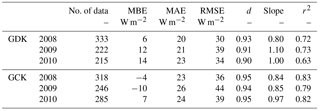
Table 1Statistical parameters for the error assessment at the study sites. Mean bias error (MBE), mean absolute error (MAE), RMSE, and d indicate mean bias error, mean absolute error, root mean square error, and index of agreement, respectively. Slope and r2 are from the linear regression analysis.
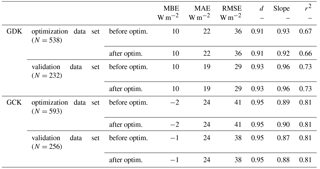
The generalization of the model can be augmented by providing the parameter optimization procedure using available flux data under wet canopy conditions. We argue that this is better than the validation using other data sets because the parameters may be site-specific (i.e., more validation does not fully guarantee the proposed model works properly everywhere). After optimizing the parameters (i.e., KL, n, and r0), the parameters changed slightly from the default values (see Appendix B for more details). Since the model results from before and after the parameter optimization were not statistically different in the error assessment, we still used the default values in a conservative way.
This method only considers the EWC from the canopy by neglecting the EWC from the trunk and stem. In addition, the interception of snow is not considered because the small amount of intercepted snowfall evaporates when the eddy covariance systems function improperly, and its melting and sublimation processes are much more complex than intercepted rainfall. To distinguish snowfall from total precipitation, the empirical discriminants in Matsuo et al. (1981) were used. This method uses air temperature and humidity near the ground surface to separate snow from rainfall because when it snows, air is not saturated and the near-ground air temperature is lower than that under rainy conditions. The result from this method should be scrutinized by comparing it with other precipitation data, which are measured at a weather station near the site.
2.3.3 Gap-filling and partitioning technique for evapotranspiration: MSH
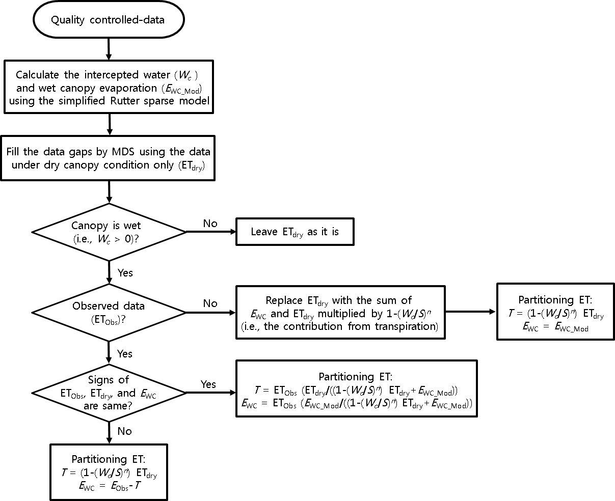
The currently used MDS is expected to underestimate and overestimate ET under wet and dry canopy conditions, respectively, due to the gap-filling without the consideration of canopy wetness (because the evaporative fraction is proportional to canopy wetness). Therefore, the gap-filling technique for ET proposed by Kang et al. (2012) was used: (1) to identify the canopy wetness, the intercepted canopy water (Wc; see Eq. 1) was calculated using the simplified Rutter sparse model; (2) all the missing gaps were filled by the MDS using the data under dry canopy conditions only (i.e., when Wc=0), which corresponds to the ET under dry canopy conditions (ETdry); (3) under wet canopy conditions (i.e., when Wc>0), the gap-filled data were replaced with the sum of the EWC estimated by the simplified Rutter sparse model (i.e., EWC_Mod) and the ETdry multiplied by (i.e., the contribution from transpiration; see Eqs. 1 and 2).
Such a gap-filled ET was partitioned into the transpiration (T or ET from the dry canopy, which approaches the actual transpiration under a dense and closed canopy conditions) and EWC as follows. When data were missing, the T was estimated as ( ETdry, while the EWC was estimated as EWC_Mod. If the data were not missing (i.e., ETObs), the partitioning procedure was divided into two parts. If the signs of ETObs, ETdry, and EWC_Mod were the same, the T was estimated by multiplying ETObs and the ratios of ( ETdry to the sum of ( ETdry and EWC_Mod (i.e., the estimated transpired fraction of ET), while the EWC was estimated by multiplying ETObs and the ratios of EWC_Mod to the sum of ( ETdry and EWC_Mod (i.e., the estimated evaporated fraction of ET). If the signs of ETObs, ETdry, and EWC_Mod were not the same, then T was estimated by ( ETdry, while the EWC was estimated by subtracting ( ETdry (i.e., the estimated T) from ETObs. The procedure regarding the MSH is described in Fig. 1.
3.1 Validation of the MSH
First, we evaluated the latent heat flux under (mostly) wet canopy conditions (λETWC, i.e., λET when ) from the MSH method (λETWC_MSH) against the observed λETWC (λETWC_Obs) at both sites from 2008 to 2010 (Fig. 2). Since the λETWC occurs in during and following rain events, open-path EC system can measure the λETWC when the instrument dries out faster than the canopy. Most of the points are near the one-to-one line. The data scattered away from the one-to-one line are characterized by large aerodynamic conductance (e.g., > 100 mm s−1) and/or large VPD (e.g., > 10 hPa).
Table 1 shows the statistical parameters for the error assessment (i.e., MBE, MAE, RMSE, d, slope, and r2; see Appendix D for more details about the error assessment). The slopes from the linear regression analysis are 0.97 ± 0.15 and 0.89 ± 0.07 with 0.69 ± 0.06 and 0.81 ± 0.02 of r2 for the GDK and GCK sites, respectively. The d values for the sites were close to 1 (0.91 ± 0.01 for the GDK and 0.95 ± 0.01 for the GCK). Compared to previous research (i.e., Kang et al., 2012), the results from the MSH were closer to the observation due to the consideration of ET from the dry canopy. One of the leading causes of the error in λETWC_MSH was identified as the discrepancy between the time when the rain occurred and the time the tipping bucket was tipped. The results from the further evaluation of the MSH using a closed-path EC system were similar to those using the open-path EC system (see the Appendix C). To validate only EWC, cross-validation using the other models (e.g., Gash sparse analytical model; Gash et al., 1995) can be attempted (e.g., Kang et al., 2012). Overall, the results from the linear regression analysis of λETWC_MSH and λETWC_Obs show that MSH can provide λETWC reasonably well for the sites.
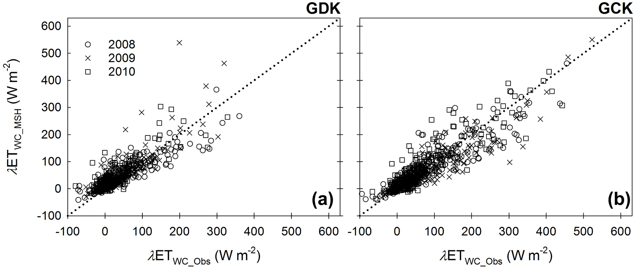
Figure 2Comparison of the latent heat flux under (mostly) wet canopy conditions (i.e., , where Wc is the intercepted canopy water and S is the canopy storage capacity) at the GDK (a) and GCK (b) sites: λETWC_Obs indicates the observed latent heat flux under wet canopy conditions (λETWC), while λETWC_MSH indicates the estimated λETWC using the MSH. The dotted line represents the 1:1 line.
3.2 Comparison between the MDS and the MSH
To evaluate the superiority of the MSH, we filled in the missing λETWC data by using the MDS (λETWC_MDS) and the MSH (λETWC_MSH). The underestimation of the λETWC_MDS was shown by the comparison with the sum of energy flux components except for latent heat flux (= net radiation + sensible heat flux + storage flux) in our previous study (Kang et al., 2012). The λEWC_mod displayed the mirrored patterns of the sum of the other energy budget components, while the λETWC_MDS was very small (mainly due to the low radiation during the rainy days). Thus, we expected that the MDS underestimates the ET since it cannot explicitly consider the key processes of wet canopy evaporation (i.e., the effects of aerodynamic conductance (ga) change and sensible heat advection; see Kang et al., 2012 for a more detailed explanation). Actually, the average annual MBEs from 2008 to 2010 were −18 ± 6 W m−2 for the GDK site and −15 ± 5 W m−2 for the GCK site, respectively. It also should be noted that some λETWC_MSH varied while λETWC_MDS was nearly constant, because (1) the λETWC_Obs rarely existed close to the missing data and (2) the MDS did not consider the effect of ga (not shown here).
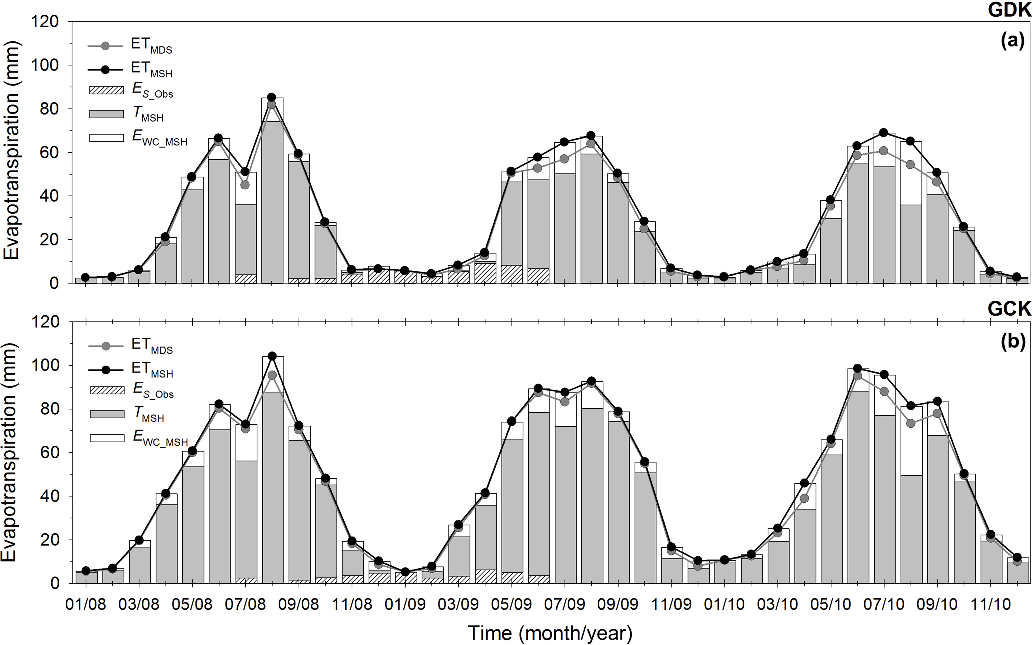
Figure 3Seasonal variation of monthly integrated evapotranspiration (ET) with the gap-filled by the MDS method (ETMDS); the ET gap-filled by the MSH method (ETMSH), transpiration and wet canopy evaporation partitioned by the MSH method (TMSH and EWC_MSH), for the GDK (a) and GCK (b) sites. ES_Obs indicates soil evaporation measured by the supplementary eddy covariance systems at the floors (adapted from Kang et al., 2009b).
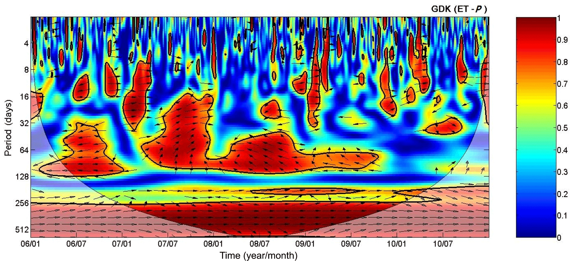
Figure 4Wavelet coherence spectrum of evapotranspiration (ET) with rainfall (P) for the GDK site. The thick solid contour is the 5 % significance level against red noise as calculated from a Monte Carlo simulation. Arrows are the relative phase angle with in-phase angle (positive correlation) pointing right, anti-phase angle (negative correlation) pointing left, and P leading ET by 90∘ pointing down. The shaded area indicates the cone of influence where the edge effects might distort the results.
Figure 3 shows the monthly ETs gap-filled by the MDS and MSH methods for the GDK and GCK sites. First, the annual ETs from the MSH method were 16–41 mm yr−1 larger than those from the MDS method, while the random uncertainties in gap-filled annual ETs were approximately 5 mm yr−1 for both sites (quantified according to Finkelstein and Sims, 2001, and Richardson and Hollinger, 2007). Significant differences were identified in June, July, August, and September during intense rainfall. The biggest difference is shown in 2010 with more frequent and larger rainfall (for the GDK, the number of rainy days is 86, 82, and 103 days and the total amount of rainfall is 1407, 1323, and 1652 mm in 2008, 2009, and 2010, respectively; such characteristics are similar to those for the GCK). In addition to taking the missing EWC from the MDS into account, the other advantage of the MSH method is that the observed ET using the eddy covariance system can be partitioned into transpiration (T) and EWC without any additional measurement. However, it can be applied to a dense canopy only, where soil evaporation is negligible. Otherwise (e.g., before leaf unfolding and after leaf fall), the T includes the error of the soil evaporation (ES). Thus, there is more separating the EWC than partitioning the ET. The annual EWC ranged from 53 to 82 mm for the GDK and 78 to 112 mm for the GCK, which occupies 14–23 and 14–19 % of the annual ET, respectively.
For quantifying the ES, the supplementary eddy covariance (EC) systems were operated at the floors of the GDK and GCK sites (Kang et al., 2009b). The annual understory ET (∼ ES) from 1 June 2008 to 31 May 2009 was 59 mm for the GDK and 43 mm for the GCK, which comprised 16 and 8 % of the annual ET, respectively. The decoupling factor (Ω, McNaughton and Jarvis, 1983) at the forest floor was ∼ 0.15 for both sites, which indicates that the ES was controlled primarily by the VPD and surface conductance (gs) rather than Rsdn. This factor also suggests that separating ES from ET using the exponential radiation extinction model to estimate the Rsdn at the forest floor and the relationship between the estimated Rsdn and the ET when the canopy is inactive (Stoy et al., 2006) can be problematic for the sites. Considering that the accurate estimation of gs is challenging, a supplementary measurement (e.g., low-level EC, lysimeter, sap-flow and isotope measurements) is a better approach for estimating ES. Using the ES measured by the low-level EC, the annual T can be estimated at 265 mm (70 % of ET) for the GDK and 448 mm (78 % of ET) for the GCK, while the EWC is estimated as 55 mm (15 % of ET) and 82 mm (14 % of ET), respectively (Fig. 3).
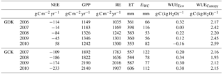
Table 2The annual CO2 and H2O budget (NEE, net ecosystem exchange; GPP, gross primary production; RE, ecosystem respiration; ET, evapotranspiration; EWC, wet canopy evaporation) and water use efficiency at the ecosystem level (WUEEco) and the canopy level (WUECanopy) for the study sites.
In the following chapters, we illustrate the advantages of the proposed technique. The benefits are caused by the gap-filling and partitioning of the H2O flux because the MSH method can take the EWC into account properly and separate them from ET, which has not yet been previously possible. We hope the following chapters draw attention to the ET partitioning.
3.3 Application: wavelet coherence analysis between ET and the rainfall
To evaluate the effect of new gap-filling, we conducted the wavelet coherence analysis between ET and rainfall for the GDK site (Fig. 4; see Hong et al., 2011, and Grinsted et al., 2004, for more details regarding the wavelet coherence analysis). From a 1- to 3-month period during the monsoon season (i.e., the intense rainy period), high correlation (i.e., red color area) was observed between ET and rainfall in 2006, 2007, 2008, and 2009. In 2007, the rainfall amount was 200 mm lower than the average level during the study period. However, the rainfall duration was the longest, and the intensity was the lowest. In 2006, 2008, and 2009, the arrow on the high correlation area pointed left. This means a negative correlation between the two variables, reflecting that the decrease in T was caused by the diminishment of Rsdn during the intense rainy period. In contrast, the arrow pointed right in 2007, indicating a positive correlation. The magnitude of enhanced EWC was greater than that of decreased T at that time and frequency (i.e., August and September, 1- to 3-month period) in 2007. Such a positive correlation between ET and rainfall with the 1- to 3-month cycle in 2007 was not reported in the study of Hong et al. (2011), which showed a negative correlation in 2006, 2007, and 2008 at that time and frequency. This can be attributed to the improvement in ET data made by the new gap-filling method (i.e., recovering the missing EWC in the general gap-filling method). During the monsoon season, the EWC compensates for (a portion of) the decreased T, and are occasionally be balanced (e.g., in 2010).
There is some circumstantial evidence which suggesting that the proposed method is more appropriate for taking EWC into account than the conventional method: (1) the ratio of the runoff and the precipitation (adapted from Choi, 2011) in 2007 was the lowest (0.60 in 2007, 0.69 ± 0.06 in the other years; i.e., the ratio of ET to precipitation was highest in 2007), while the Rsdn (main controlling factor of T) was lowest (4.52 GJ m−2 in 2007, 4.77 ± 0.08 GJ m−2 in the other years) due to the longest rainfall duration, (2) the interannual variabilities of the estimated catchment-scale annual ET (i.e., precipitation–runoff) and ET from the MDS method occurred in opposite directions (similarly to T from the MSH method).
3.4 Application: water use efficiency at the ecosystem level and the canopy level
Water use efficiency (WUE) can be defined in various forms such as An∕gst (intrinsic WUE; An: net assimilation; gst: stomatal conductance; An= NPP), An∕T (instantaneous WUE), (1+Φw)] (integrated WUE; Φc: fraction of assimilated carbon lost in respiration; Φw: fraction of total water loss from non-photosynthetic parts of the plant or through open stomata at night), the GPP ∕ T (canopy-level WUE), NPP ∕ ET (stand-level WUE), and GPP ∕ ET (ecosystem-level WUE; Seibt et al., 2008; Ito and Inatomi, 2012; Ponton et al., 2006), because the spatiotemporal scale and measurement method are research-specific. Based on the original definition of WUE (i.e., the ratio of CO2 flux to H2O flux), we redefined the annual ecosystem-level WUE (WUEEco) and the annual canopy-level WUE (WUECanopy) as ΣNEP ∕ ΣET and ΣNPP ∕ ΣT, respectively. For estimating ΣNPP and ΣT simply, we used 0.45 as the ratio of the NPP to GPP for both sites (Waring et al., 1998), and 0.156 and 0.075 as the ratios of ES to ET for the GDK and GCK, respectively (Kang et al., 2009b). From 2006 to 2010, WUEEco (WUECanopy) ranged from −0.16 (2.17) to 0.32 (2.59) g C (kg H2O)−1 for the GDK site and from 0.20 (1.93) to 0.38 (2.16) g C (kg H2O)−1 for the GCK site (Table 2). Considering the increasing trend of NEE and GPP for the GCK site, we identified that the interannual variabilities of WUEEco and WUECanopy occurred in opposite directions for both sites. It was primarily caused by EWC being enhanced in 2007 and 2010 due to the weakest rainfall intensity and the largest rainfall amount, respectively. Overall, such partitioning of the total ET into EWC, T, and ES enables us to understand better how ET responds to environmental changes and the how water cycle is connected to the carbon cycle in a forest ecosystem.
The new technique proposed in this study for gap-filling and partitioning of H2O eddy fluxes has a special feature: two existing methods were merged into a new method. The marginal distribution sampling (MDS) method and the simplified Rutter spars model have been merged into the model–statistics hybrid (MSH) method. Such a strategy increases the strength of the original methods while making up for their weaknesses. Thus, further improvement is necessary and forthcoming. The MSH method can be applied to tropical forests because tropical forests also share three properties of temperate forests (i.e., extensive, dense, and tall). However, applying the methods to grasslands may need further validation.
Flux tower data (including the metadata) until 2008 are available in the AsiaFlux database (https://db.cger.nies.go.jp/asiafluxdb/, AsiaFlux, 2006). The data for the other years are available upon request from the first author.
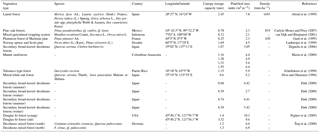
The rainfall interception is sensitive to the change of canopy storage capacity (S) and vegetation fraction (σf, i.e., 1 minus the gap fraction; e.g., Shi et al., 2010). One of the characteristics common among the temperate forests considered in this study is a dense canopy. It means that the vegetation fractions in the forests are close to 1 (except before leaf unfolding and after leaf fall periods). Moreover, the gap fraction can be measured using a plant canopy analyzer with relative ease. Therefore, the error of the result from the model is mostly derived from the parameterization of S (see Appendix B for more detailed information). The canopy storage capacity is affected by not only leaf area but also the other factors such as leaf shape, leaf angle, leaf/shoot clumping, and hydrophobicity (water repellency) of a leaf (e.g., Crockford and Richardson, 2000). Additionally, the relationships between S and these characteristics are changeable according to meteorological conditions (e.g., the wind, rainfall intensity), which make the parameterization of S difficult (e.g., Dunkerley, 2009). Therefore, we used the simple parameterization of S of VIC LSM (i.e., leaf (or plant) area index, where KL=0.2; Liang et al., 1994) and evaluated whether the parameterization was reasonable or not. The relationships between the leaf area index (LAI) and S in previous studies are presented in Fig. A1, indicating that the parameterization in VIC LSM (i.e., KL=0.2) is reasonable, and the KL ranges from 0.1 to 0.3. Further studies on the parameterization of S using leaf structure (e.g., leaf shape, leaf angle, leaf/shoot clumping) would be worth conducting for more accurate estimation of wet canopy evaporation.
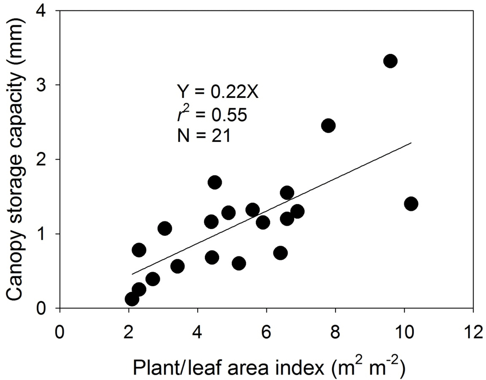
Figure A1Relationship between canopy storage capacity and plant/leaf area index (the data obtained from Table A1).
Table A1Review of the canopy storage capacity for wet canopy evaporation modeling in previous studies.
In the simplified Rutter sparse model (Liang et al., 1994), there are many parameters (e.g., σf, S, n, ra, and r0) for estimating the wet canopy evaporation (EWC) and the intercepted canopy water (Wc). Since the model results may be sensitive to the parameters, and the parameters may be site-specific, the parameter optimization using available flux data under wet canopy conditions should be accompanied by the model for the generalization of the model. Considering that the gap-filling and partitioning are a kind of interpolation and extrapolation (i.e., identifying relationships between a target flux and its drivers, and interpolating and extrapolating the relationships), it is an appropriate strategy for the gap-filling and partitioning of evapotranspiration using the model.
First, we conducted a sensitivity test of the model to the parameters (i.e., k, KL, n, and r0) using the data set in 2008 (change in EWC (%) ; EWC_default: annually integrated EWC simulated with default parameters; EWC_perturb: annually integrated EWC simulated after a change in each parameter. Only one parameter is changed one at a time, while other parameters are held constant; e.g., Shi et al., 2010). Before testing the sensitivity, we set the lower/upper boundaries (and default values) based on literature reviews: k=0.3 ∼ 1.5 (Jones, 2013; the default values of k are 0.75 and 0.485 for the GDK and GCK, respectively; these values were obtained from the actual measurement using a plant canopy analyzer, LAI-2000 from LI-COR, Inc.); KL=0.1 ∼ 0.3 (see Appendix B; default value of KL is 0.2, Dickinson, 1984); n=0.5 ∼ 1 (Chen and Dudhia, 2001; Liang et al., 1994; Valente et al., 1997; the default value of n is two-thirds: Deardorff, 1978); r0= 0 (for short vegetation) and ∼ 2 s m−1 (for tall vegetation; Perrier, 1975; Rana et al., 1994; the default value of r0 is 2: Perrier, 1975). KL is the most influential parameter (Fig. B1), implying that we should take great care to minimize its parameter estimation error. Using a small number of the observed latent heat flux data under wet canopy conditions (when ) from 2008 to 2010, we optimized the parameters except k (because we obtained the k from the actual measurement) towards minimizing the root mean square error of the method (using the bound constrained optimization code in MATLAB®, “fminsearchbnd.” http://kr.mathworks.com/matlabcentral/fileexchange/8277-fminsearchbnd–fminsearchcon). We randomly divided the available data set into the data sets for parameter optimization and validation (i.e., validation after optimization). The ratio of the optimization–validation data sets was arbitrarily set to 7:3. Table B1 shows the model parameters and the statistical parameters for the error assessment before and after the parameter optimization. After the optimization, the parameters were slightly different from the default values. However, we still used the default values conservatively since the model results from before and after the optimization were not statistically different in the error assessment.
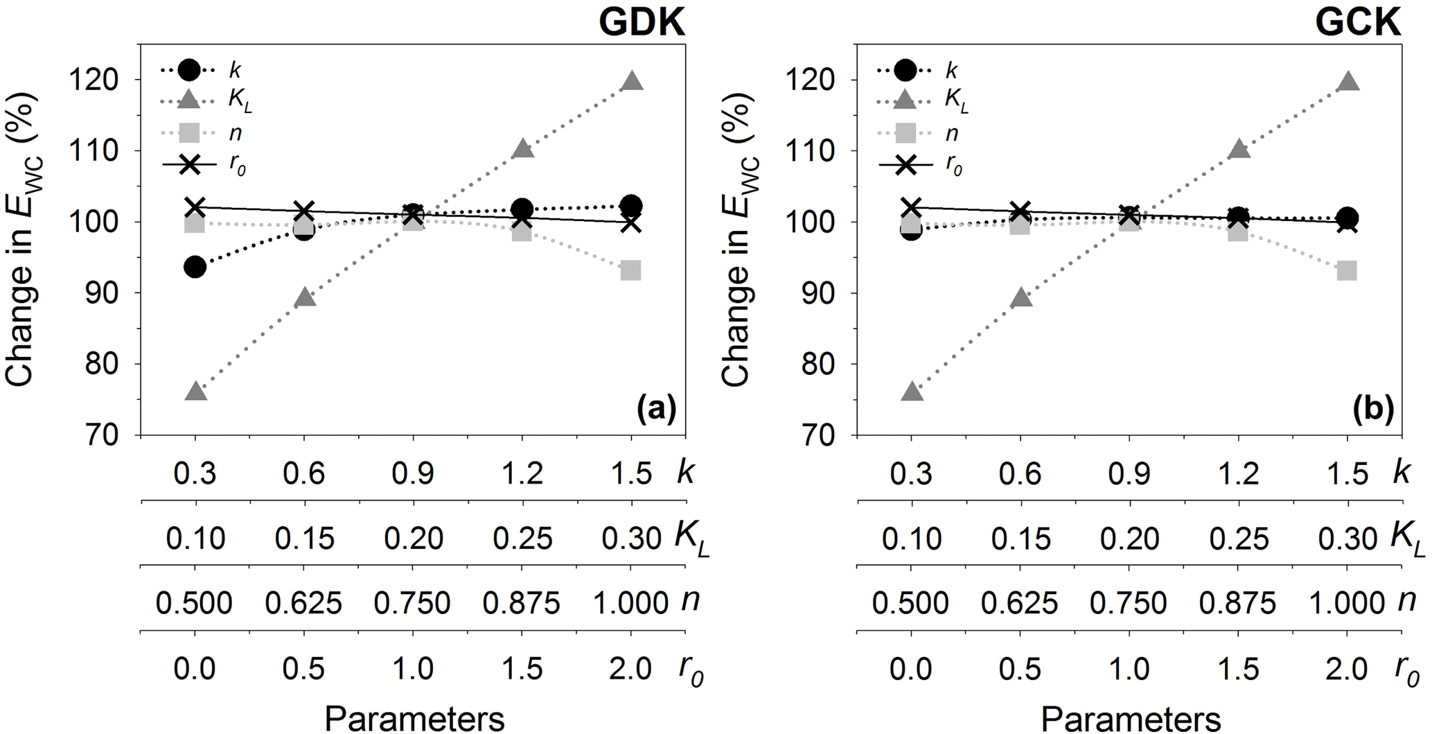
Figure B1Sensitivity test of the wet canopy evaporation model to the parameters (i.e., k, KL, n, and r0).
Table B1Statistical parameters before and after the parameter optimization for the error assessment at the study sites. MBE, MAE, RMSE, and d indicate mean bias error, mean absolute error, root mean square error, and index of agreement, respectively. Slope and r2 are from the linear regression analysis. The default values of KL, n, and r0 were 0.2 (0.2), 2∕3 (2∕3), and 2 (2) for the GDK (GCK), respectively. After the optimization, those values changed to 0.1966 (0.2314), 0.7279 (0.6930), and 2 (2) for the GDK (GCK), respectively.
For further evaluation of the MSH method, we conducted a commercialized closed-path infrared gas analyzer with the heated tube (model EC155, Campbell Scientific Inc., Logan, Utah, USA) from 18 August 2015 to 25 October 2015 for the GDK site. The open- and closed-path gas analyzers shared the one sonic anemometer. We applied the MSH to the latent heat fluxes (λET) from the open-path eddy covariance (EC) system for gap-filling the λET under wet canopy conditions, and the frequency response correction (Fratini et al., 2012) to the λET from the closed-path EC system for correcting the tube attenuation effect especially under high relative humidity (RH) conditions. Then, we compared the λET (mostly) wet canopy conditions (λETWC, i.e., λET when ) from the MSH (λETWC_MSH_OP) against the observed λETWC from the closed-path EC system (λETWC_Obs_CP) similar to Sect. 3.1 (Fig. C1).
Before the comparison, it should be noted that the data retrieval rate under wet canopy conditions of the closed-path EC system was 50 % higher than that of the open-path EC system; however, there were still data missing for a considerable period despite the use of the closed-path gas analyzer. The lack of data was mainly caused by the malfunction of the sonic anemometer and the unsatisfactory conditions for EC measurement (e.g., nonstationary and unfavorable turbulent conditions developed). The results of the error assessment (i.e., 10 W m−2 of MBE, 19 W m−2 of MAE, 29 W m−2 of RMSE, 0.90 of d, 1.04 of slope, 0.68 of r2) were within the ranges of those from the comparison between the λETWC_MSH_OP and the λETWC_Obs in Sect. 3.1 (i.e., the case of the open-path EC system). Overall, such results imply the robustness of the MSH method as well as the necessity of appropriate λETWC gap-filling method (e.g., MSH) when measuring using a closed-path EC system, as in the case of an open-path EC system.
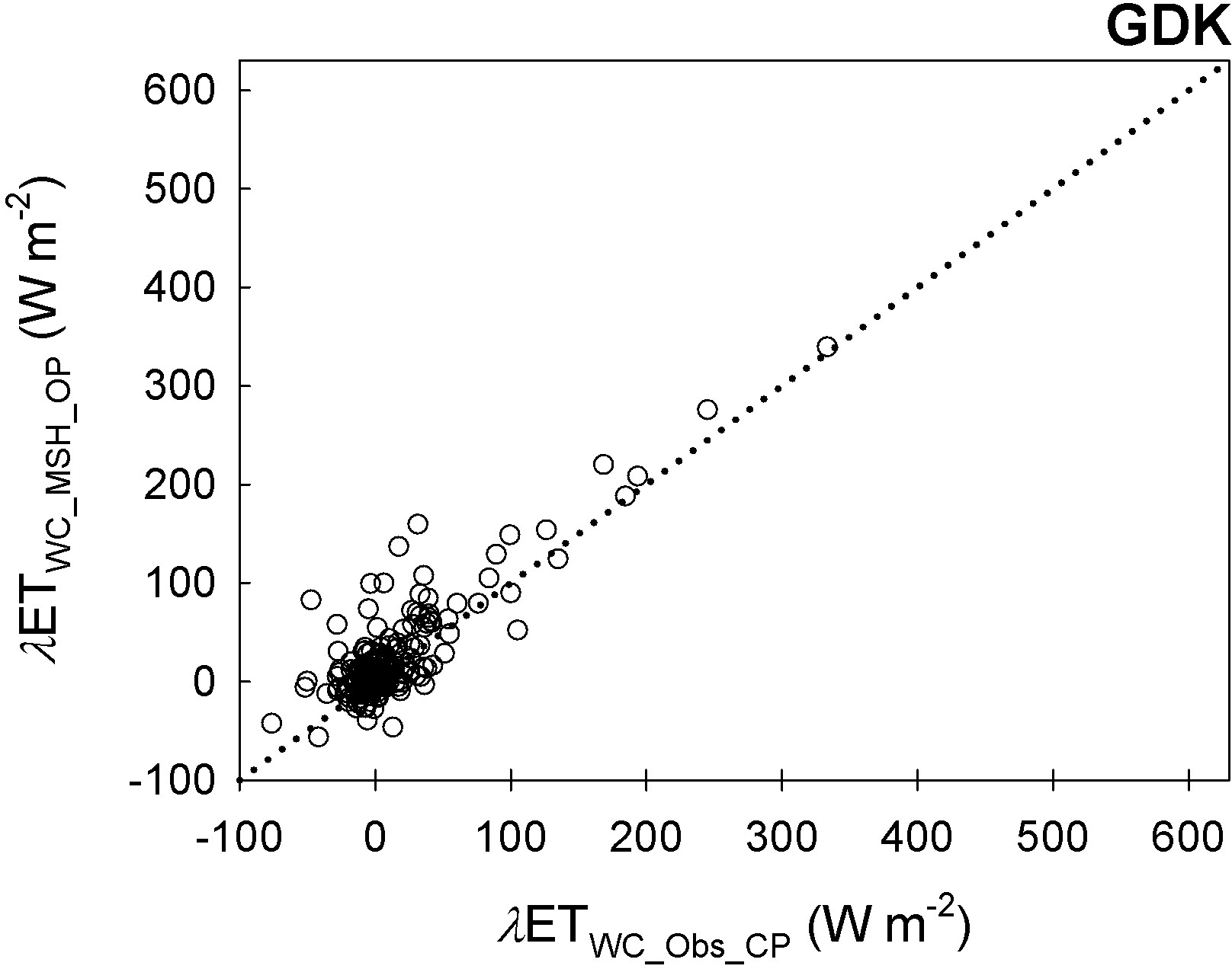
Figure C1Comparison of the latent heat flux under (mostly) wet canopy conditions (i.e., , where Wc is the intercepted canopy water and S is the canopy storage capacity) at the GDK site: λETWC_Obs_CP indicates the observed latent heat flux under wet canopy conditions (λETWC) from a closed-path eddy covariance (EC) system, while λETWC_MSH_OP indicates the estimated λETWC from an open-path EC system using the MSH method. The dotted line represents the 1:1 line.
In order to evaluate the latent heat flux under wet canopy conditions obtained from the MSH method, we compared it against the observed data using four statistical measures, following Willmott and Matsuura (2005). Mean bias error is the average of the residuals. Mean absolute error is the average of the absolute values of the residuals. A large deviation from zero implies that the estimation generally overestimates or underestimates compared to the observed values. We also considered root mean squared error (RMSE) which is often reported with MAE because RMSE is more sensitive to large errors than MAE.
MBE, MAE, and RMSE give estimates of the average error, but none of them provide information about the relative size of the average difference. Thus, we further considered an additional index of agreements (d), following Willmott (1982):
where and (where overbar is an averaging operator). It ranges from 0 to 1, where 0 is for complete disagreement and 1 for complete agreement between the observation and the estimates. It is both a relative and bounded measure that can be widely applied in order to make a cross-comparison between models.
The authors declare that they have no conflict of interest.
This work was supported by the Korea Meteorological Administration Research and Development Program under grant KMIPA-2015-2023, by the Weather Information Service Engine Program of the Korea Meteorological Administration under grant KMIPA-2012-0001-2, and by the R&D Program for Forest Science Technology (project no. 2017099A00-1719-BB01) of the Korea Forest Service (Korea Forestry Promotion Institute). We thank Hyojung Kwon, Jinkyu Hong, Jaeill Yoo, Juyeol Yun, and Je-woo Hong for their helpful support in the data collection and other logistics. Wavelet tools used in this study benefited from Grinsted et al. (2004).
Edited by: Georg Wohlfahrt
Reviewed by: two anonymous referees
Aboal, J. R., Jiménez, M. S., Morales, D., and Hernández, J. M.: Rainfall interception in laurel forest in the Canary Islands, Agr. Forest Meteorol., 97, 73–86, 1999.
AsiaFlux: AsiaFlux database, available at: https://db.cger.nies.go.jp/asiafluxdb/ (last access: 31 January 2018), 2006–2008.
Baldocchi, D. D., Hicks, B. B., and Meyers, T. P.: Measuring biosphere-atmosphere exchanges of biologically related gases with micrometeorological methods, Ecology, 69, 1331–1340, 1988.
Carlyle-Moses, D. E. and Price, A. G.: Modelling canopy interception loss from a Madrean pine-oak stand, northeastern Mexico, Hydrol. Process., 21, 2572–2580, 2007.
Choi, H. T.: Effect of forest growth and thinning on the long-term water balance in a coniferous forest, Korean J. Agr. Forest Meteorol., 13, 157–164, 2011 (in Korean with English abstract).
Crockford, R. H. and Richardson, D. P.: Partitioning of rainfall into throughfall, stemflow and interception effect of forest type, ground cover and climate, Hydrol. Process., 14, 2903–2920, 2000.
Daikoku, K., Hattori, S., Deguchi, A., Aoki, Y., Miyashita, M., Matsumoto, K., Akiyama, J., Iida, S., Toba, T., and Fujita, Y.: Influence of evaporation from the forest floor on evapotranspiration from the dry canopy, Hydrol. Process., 22, 4083–4096, 2008.
Deardorff, J. W.: Efficient prediction of ground surface temperature and moisture, with inclusion of a layer of vegetation, J. Geophys. Res., 83, 1889–1903, 1978.
Deguchi, A., Hattori, S., and Park, H. T.: The influence of seasonal changes in canopy structure on interception loss: Application of the revised Gash model, J. Hydrol., 318, 80–102, 2006.
Dickinson, R. E.: Modelling evapotranspiratio for three-dimensional global climate models, in Climate Processes and Climate Sensitivity, Geophys. Monogr. Set., 29, edited by: Hansen, J. E. and Takahashi, T., AGU, Washington DC, 58–72, 1984.
Dunkerley, D. L.: Evaporation of impact water droplets in interception processes: Historical precedence of the hypothesis and a brief literature overview, J. Hydrol., 376, 599–604, 2009.
Finkelstein, P. L. and Sims, P. F.: Sampling error in eddy correlation flux measurements, J. Geophys. Res.-Atmos., 106, 3503–3509, 2001.
Fratini, G., Ibrom, A., Arriga, N., Burba, G., and Papale, D.: Relative humidity effects on water vapour fluxes measured with closed-path eddy-covariance systems with short sampling lines, Agr. Forest Meteorol., 165, 53–63, 2012.
Gash, J. H., Lloyd, C. R., and Lachaud, G.: Estimating sparse forest rainfall interception with an analytical model, J. Hydrol., 170, 79–86, 1995.
Goodrich, J. P., Oechel, W. C., Gioli, B., Moreaux, V., Murphy, P. C., Burba, G., and Zona, D.: Impact of different eddy covariance sensors, site set-up, and maintenance on the annual balance of CO2 and CH4 in the harsh Arctic environment, Agr. Forest Meteorol., 228, 239–251, 2016.
Grinsted, A., Moore, J. C., and Jevrejeva, S.: Application of the cross wavelet transform and wavelet coherence to geophysical time series, Nonlin. Processes Geophys., 11, 561–566, https://doi.org/10.5194/npg-11-561-2004, 2004.
Hong, J. and Kim, J.: Impact of the Asian monsoon climate on ecosystem carbon and water exchanges: a wavelet analysis and its ecosystem modeling implications, Glob. Change Biol., 17, 1900–1916, 2011.
Hong, J., Lee, D., and Kim, J.: Lessons from FIFE (First ISLSCP Field Experiment) inscaling issues of surface fluxes at Gwangneung supersite, Korean J. Agr. Forest Meteorol. 7, 4–14, 2005 (in Korean with English abstract).
Hong, J., Kim, J., Lee, D., and Lim, J. H.: Estimation of the storage and advection effects on H2O and CO2 exchanges in a hilly KoFlux forest catchment, Water Resour. Res., 44, W01426, https://doi.org/10.1029/2007WR006408, 2008.
Hong, J., Kwon, H.-J., Lim, J.-H., Byun, Y.-H., Lee, J.-H., and Kim, J.: Standardization of KoFlux eddy-covariance data processing, Korean J. Agr. Forest Meteorol., 11, 19–26, 2009 (in Korean with English abstract).
Hu, Z., Yu, G., Zhou, Y., Sun, X., Li, Y., Shi, P., Wang, Y., Song, X., Zheng, Z., and Zhang, L.: Partitioning of evapotranspiration and its controls in four grassland ecosystems: Application of a two-source model, Agr. Forest Meteorol., 149, 1410–1420, 2009.
Hwang, Y., Ryu, Y., Kimm, H., Jiang, C., Lang, M., Macfarlane, C., and Sonnentag, O.: Correction for light scattering combined with sub-pixel classification improves estimation of gap fraction from digital cover photography, Agr. Forest Meteorol., 222, 32–44, 2016.
Ibrom, A., Dellwik, E., Flyvbjerg, H., Jensen, N. O., and Pilegaard, K.: Strong low-pass filtering effects on water vapour flux measurements with closed-path eddy correlation systems, Agr. Forest Meteorol., 147, 140–156, 2007.
Ito, A. and Inatomi, M.: Water-use efficiency of the terrestrial biosphere: a model analysis focusing on interactions between the global carbon and water cycles, J. Hydrometeorol., 13, 681–694, 2012.
Jones, H. G.: Plants and microclimate: a quantitative approach to environmental plant physiology, Cambridge university press, 9–46, 2013.
Kang, M., Park, S., Kwon, H., Choi, H. T., Choi, Y. J., and Kim, J.: Evapotranspiration from a deciduous forest in a complex terrain and a heterogeneous farmland under monsoon climate, Asia-Pac., J. Atmos. Sci., 45, 175–191, 2009a.
Kang, M., Kwon, H., Lim, J.-H., and Kim, J.: Understory evapotranspiration measured by eddy-covariance in Gwangneung deciduous and coniferous forests, Korean J. Agr. Forest Meteorol., 11, 233–246, 2009b (in Korean with English abstract).
Kang, M., Kwon, H., Cheon, J. H., and Kim, J.: On estimating wet canopy evaporation from deciduous and coniferous forests in the Asian monsoon climate, J. Hydrometeorol., 13, 950–965, 2012.
Kang, M., Kim, J., Kim, H.-S., Thakuri, B. M., and Chun, J.-H.: On the nighttime correction of CO2 flux measured by eddy covariance over temperate forests in complex terrain, Korean J. Agr. Forest Meteorol., 16, 233–245, 2014 (in Korean with English abstract).
Kang, M., Thakuri, M. B., Kim, J., Chun, J., and Cho, C.: A modification of the moving point test method for nighttime eddy flux filtering on hilly and complex terrain, Abstract B41B-0404 presented at 2016 Fall Meeting, AGU, San Francisco, Calif., 2016.
Kang, M., Ruddell, B. L., Cho, C., Chun, J., and Kim, J.: Identifying CO2 advection on a hill slope using information flow, Agr. Forest Meteorol., 232, 265–278, 2017.
Kim, J. and Verma, S. B.: Components of surface energy balance in a temperate grassland ecosystem, Bound.-Lay. Meteorol., 51, 401–417, 1990.
Kim, J., Lee, D., Hong, J., Kang, S., Kim, S.-J., Moon, S.-K., Lim, J.-H., Son, Y., Lee, J., Kim, S., Woo, N., Kim, K., Lee, B., Lee, B.-L., and Kim, S.: HydroKorea and CarboKorea: cross-scale studies of ecohydrology and biogeochemistry in a heterogeneous and complex forest catchment of Korea, Ecol. Res., 21, 881–889, 2006.
Kwon, H., Park, T.-Y., Hong, J., Lim, J.-H., and Kim, J.: Seasonality of Net Ecosystem Carbon Exchang in Two Major Plant Functional Types in Korea, Asia-Pac., J. Atmos. Sci., 45, 149–163, 2009.
Lankreijer, H., Lundberg, A., Grelle, A., Lindroth, A., and Seibert, J.: Evaporation and storage of intercepted rain analysed by comparing two models applied to a boreal forest, Agr. Forest Meteorol., 98–99, 595–604, 1999.
Liang, X., Lettenmaier, D. P., Wood, E. F., and Burges, S. J.: A simple hydrologically based model of land surface water and energy fluxes for general circulation models, J. Geophys. Res.-Atmos., 99, 14415–14428, 1994.
Macfarlane, C., Hoffman, M., Eamus, D., Kerp, N., Higginson, S., McMurtrie, R., and Adams, M.: Estimation of leaf area index in eucalypt forest using digital photography, Agr. Forest Meteorol., 143, 176–188, 2007.
Marin, C. T., Bouten, W., and Sevink, J.: Gross rainfall and its partitioning into throughfall, stemflow and evaporation of intercepted water in four forest ecosystems in western Amazonia, J. Hydrol., 237, 40–57, 2000.
Matsuo, T., Sasyo, Y., and Sato, Y.: Relationship between types of precipitation on the ground and surface meteorological elements, J. Meteorol. Soc. Jpn. Ser. II, 59, 462–476, 1981.
McNaughton, K. G. and Jarvis, P. G.: Predicting effects of vegetation changes on transpiration and evaporation, Water Deficits and Plant Growth, 7, 1–47, 1983.
Richardson, A. D. and Hollinger, D. Y.: A method to estimate the additional uncertainty in gap-filled NEE resulting from long gaps in the CO2 flux record, Agr. Forest Meteorol., 147, 199–208, 2007.
Moon, S.-K., Park, S.-H., Hong, J., and Kim, J.: Spatial characteristics of Gwangneung forest site based on high resolution satellite images and DEM, Korean J. Agr. Forest Meteorol., 7, 115–123, 2005 (in Korean with English abstract).
Park, H.: Physical characteristics of heat and water exchange processes between vegetation and the atmosphere in a deciduous broad-leaved forest, Nagoya University, 2000.
Papale, D.: Data gap filling, in: Eddy Covariance, Springer Netherlands, 159–172, 2012.
Papale, D. and Valentini, R.: A new assessment of European forests carbon exchanges by eddy fluxes and artificial neural network spatialization, Glob. Change Biol., 9, 525–535, 2003.
Papale, D., Reichstein, M., Aubinet, M., Canfora, E., Bernhofer, C., Kutsch, W., Longdoz, B., Rambal, S., Valentini, R., Vesala, T., and Yakir, D.: Towards a standardized processing of Net Ecosystem Exchange measured with eddy covariance technique: algorithms and uncertainty estimation, Biogeosciences, 3, 571–583, https://doi.org/10.5194/bg-3-571-2006, 2006.
Perrier, A.: Etude physique de l'évapotranspiration dans les conditions naturelles. III. Evapotranspiration réelle et potentielle des couverts végétaux, in: Annales agronomiques, 1975.
Ponton, S., Flanagan, L. B., Alstad, K. P., Johnson, B. G., Morgenstern, K., Kljun, N., Black, T. A., and Barr, A. G.: Comparison of ecosystem water-use efficiency among Douglas-fir forest, aspen forest and grassland using eddy covariance and carbon isotope techniques, Glob. Change Biol., 12, 294–310, 2006.
Pypker, T. G., Bond, B. J., Link, T. E., Marks, D., and Unsworth, M. H.: The importance of canopy structure in controlling the interception loss of rainfall: Examples from a young and an old-growth Douglas-fir forest, Agr. Forest Meteorol., 130, 113–129, 2005.
Rana, G., Katerji, N., Mastrorilli, M., and El Moujabber, M.: Evapotranspiration and canopy resistance of grass in a Mediterranean region, Theor. Appl. Climatol., 50, 61–71, 1994.
Reichstein, M., Falge, E., Baldocchi, D., Papale, D., Aubinet, M., Berbigier, P., Bernhofer, C., Buchmann, N., Gilmanov, T., Granier, A., Grunwald, T., Havrankova, K., Ilvesniemi, H., Janous, D., Knohl, A., Laurila, T., Lohila, A., Loustau, D., Matteucci, G., Meyers, T., Miglietta, F., Ourcival, J.-M., Pumpanen, J., Rambal, S., Rotenberg, E., Sanz, M., Tenhunen, J., Seufert, G., Vaccari, F., Vesala, T., Yakir, D., and Valentini, R.: On the separation of net ecosystem exchange into assimilation and ecosystem respiration: review and improved algorithm, Glob. Change Biol., 11, 1424–1439, https://doi.org/10.1111/j.1365-2486.2005.001002.x, 2005.
Reichstein, M., Stoy, P. C., Desai, A. R., Lasslop, G., and Richardson, A. D.: Partitioning of net fluxes, in: Eddy Covariance, Springer Netherlands, 263–289, 2012.
Richardson, A. D. and Hollinger, D. Y.: A method to estimate the additional uncertainty in gap-filled NEE resulting from long gaps in the CO2 flux record, Agr. Forest Meteorol., 147, 199–208, 2007.
Schellekens, J., Scatena, F. N., Bruijnzeel, L. A., and Wickel, A. J.: Modelling rainfall interception by a lowland tropical rain forest in northeastern Puerto Rico, J. Hydrol., 225, 168–184, 1999.
Seibt, U., Rajabi, A., Griffiths, H., and Berry, J. A.: Carbon isotopes and water use efficiency: sense and sensitivity, Oecologia, 155, https://doi.org/10.1007/S00442-007-0932-7, 2008.
Shi, Z., Wang, Y., Xu, L., Xiong, W., Yu, P., Gao, J., and Zhang, L.: Fraction of incident rainfall within the canopy of a pure stand of Pinus armandii with revised Gash model in the Liupan Mountains of China, J. Hydrol., 385, 44–50, https://doi.org/10.1016/j.jhydrol.2010.02.003, 2010.
Shuttleworth, W., Leuning, R., Black, T., Grace, J., Jarvis, P., Roberts, J., and Jones, H.: Micrometeorology of temperate and tropical forest, Philos. T. R. Soc. B, 324, 299–334, 1989.
Silva, I. C. and Okumura, T.: Rainfall partitioning in a mixed white oak forest with dwarf bamboo undergrowth, J. Environ. Hydrol., 4, XIII–XIV, 1996.
Šraj, M., Brilly, M., and Mikoš, M.: Rainfall interception by two deciduous Mediterranean forests of contrasting stature in Slovenia, Agr. Forest Meteorol., 148, 121–134, 2008.
Stoy, P. C., Katul, G. G., Siqueira, M. B. S., Juang, J. Y., Novick, K. A., McCarthy, H. R., Oishi, A. C., Uebelherr, J. M., Kim, H. S., and Oren, R.: Separating the effects of climate and vegetation on evapotranspiration along a successional chronosequence in the southeastern US, Glob. Change Biol., 12, 2115–2135, https://doi.org/10.1111/j.1365-2486.2006.01244.x, 2006.
Thom, A. S.: Momentum, Mass, and Heat Exchange of Vegetation, Q. J. Roy. Meteor. Soc., 98, 124–134, 1972.
Valente, F., David, J. S., and Gash, J. H. C.: Modelling interception loss for two sparse eucalypt and pine forests in central Portugal using reformulated Rutter and Gash analytical models, J. Hydrol., 190, 141–162, 1997.
Van Dijk, A. I. J. M. and Bruijnzeel, L. A.: Modelling rainfall interception by vegetation of variable density using an adapted analytical model. Part 2. Model validation for a tropical upland mixed cropping system, J. Hydrol., 247, 239–262, 2001.
van Gorsel, E., Delpierre, N., Leuning, R., Black, A., Munger, J. W., Wofsy, S., Aubinet, M., Feigenwinter, C., Beringer, J., and Bonal, D.: Estimating nocturnal ecosystem respiration from the vertical turbulent flux and change in storage of CO2, Agr. Forest Meteorol., 149, 1919–1930, 2009.
Waring, R., Landsberg, J., and Williams, M.: Net primary production of forests: a constant fraction of gross primary production?, Tree Physiol., 18, 129–134, 1998.
Webb, E. K., Pearman, G. I., and Leuning, R.: Correction of flux measurements for density effects due to heat and water vapour transfer, Q. J. R. Meteor. Soc., 106, 85–100, https://doi.org/10.1002/qj.49710644707, 1980.
Wilczak, J., Oncley, S., and Stage, S.: Sonic Anemometer Tilt Correction Algorithms, Bound.-Lay. Meteorol., 99, 127–150, 2001.
Willmott, C. J.: Some comments on the evaluation of model performance, B. Am. Meteorol. Soc., 63, 1309–1313, 1982.
Willmott, C. J. and Matsuura, K.: Advantages of the mean absolute error (MAE) over the root mean square error (RMSE) in assessing average model performance, Clim. Res., 30, 79–82, https://doi.org/10.3354/cr030079, 2005.
Wilson, K. B., Hanson, P. J., Mulholland, P. J., Baldocchi, D. D., and Wullschleger, S. D.: A comparison of methods for determining forest evapotranspiration and its components: sap-flow, soil water budget, eddy covariance and catchment water balance, Agr. Forest Meteorol., 106, 153–168, 2001.
Yepez, E. A., Williams, D. G., Scott, R. L., and Lin, G.: Partitioning overstory and understory evapotranspiration in a semiarid savanna woodland from the isotopic composition of water vapor, Agr. Forest Meteorol., 119, 53–68, 2003.
Yoo, J., Lee, D., Hong, J., and Kim, J.: Principles and Applications of Multi-Level H2O/CO2 Profile Measurement System, Korean J. Agr. Forest Meteorol., 11, 27–38, 2009 (in Korean with English abstract).
Yuan, R., Kang, M, Park, S., Hong, J., Lee, D., and Kim, J.: The effect of coordinate rotation on the eddy covariance flux estimation in a hilly KoFlux forest catchment, Korean J. Agr. Forest Meteorol., 9, 100–108, 2007.
Yuan, R., Kang, M., Park, S., Hong, J., Lee, D., and Kim, J.: Expansion of the planar-fit method to estimate flux over complex terrain, Meteorol. Atmos. Phys., 110, 123–133, 2011.
- Abstract
- Introduction
- Materials and methods
- Results and discussion
- Conclusions
- Data availability
- Appendix A: Parameterizations of canopy storage
- Appendix B: Sensitivity test and parameter optimization of the wet canopy evaporation model
- Appendix C: Further evaluation of the MSH using a closed-path EC system
- Appendix D: Error assessment
- Competing interests
- Acknowledgements
- References