the Creative Commons Attribution 4.0 License.
the Creative Commons Attribution 4.0 License.
 | 05 Oct 2018
An intercomparison of oceanic methane and nitrous oxide measurements
Hermann W. Bange
Damian L. Arévalo-Martínez
Jonathan Barnes
Alberto V. Borges
Ian Brown
John L. Bullister
Macarena Burgos
David W. Capelle
Michael Casso
Mercedes de la Paz
Laura Farías
Lindsay Fenwick
Sara Ferrón
Gerardo Garcia
Michael Glockzin
David M. Karl
Annette Kock
Sarah Laperriere
Cliff S. Law
Cara C. Manning
Andrew Marriner
Jukka-Pekka Myllykangas
John W. Pohlman
Andrew P. Rees
Alyson E. Santoro
Philippe D. Tortell
Robert C. Upstill-Goddard
David P. Wisegarver
Gui-Ling Zhang
Gregor Rehder
Large-scale climatic forcing is impacting oceanic biogeochemical cycles and is expected to influence the water-column distribution of trace gases, including methane and nitrous oxide. Our ability as a scientific community to evaluate changes in the water-column inventories of methane and nitrous oxide depends largely on our capacity to obtain robust and accurate concentration measurements that can be validated across different laboratory groups. This study represents the first formal international intercomparison of oceanic methane and nitrous oxide measurements whereby participating laboratories received batches of seawater samples from the subtropical Pacific Ocean and the Baltic Sea. Additionally, compressed gas standards from the same calibration scale were distributed to the majority of participating laboratories to improve the analytical accuracy of the gas measurements. The computations used by each laboratory to derive the dissolved gas concentrations were also evaluated for inconsistencies (e.g., pressure and temperature corrections, solubility constants). The results from the intercomparison and intercalibration provided invaluable insights into methane and nitrous oxide measurements. It was observed that analyses of seawater samples with the lowest concentrations of methane and nitrous oxide had the lowest precisions. In comparison, while the analytical precision for samples with the highest concentrations of trace gases was better, the variability between the different laboratories was higher: 36 % for methane and 27 % for nitrous oxide. In addition, the comparison of different batches of seawater samples with methane and nitrous oxide concentrations that ranged over an order of magnitude revealed the ramifications of different calibration procedures for each trace gas. Finally, this study builds upon the intercomparison results to develop recommendations for improving oceanic methane and nitrous oxide measurements, with the aim of precluding future analytical discrepancies between laboratories.
- Article
(1402 KB) -
Supplement
(574 KB) - BibTeX
- EndNote


The increasing mole fractions of greenhouse gases in the Earth's atmosphere are causing long-term climate change with unknown future consequences. Two greenhouse gases, methane and nitrous oxide, together contribute approximately 23 % of total radiative forcing attributed to well-mixed greenhouse gases (Myhre et al., 2013). It is imperative that the monitoring of methane and nitrous oxide in the Earth's atmosphere is accompanied by measurements at the Earth's surface to better inform the sources and sinks of these climatically important trace gases. This includes measurements of dissolved methane and nitrous oxide in the marine environment, which is an overall source of both gases to the overlying atmosphere (Nevison et al., 1995; Anderson et al., 2010; Naqvi et al., 2010; Freing et al., 2012; Ciais et al., 2014).
Oceanic measurements of methane and nitrous oxide are conducted as part of established time series locations, along hydrographic survey lines, and during disparate oceanographic expeditions. Within low-latitude to midlatitude regions of the open ocean, the surface waters are frequently slightly supersaturated with respect to atmospheric equilibrium for both methane and nitrous oxide. There is typically an order of magnitude range in concentration along a vertical water-column profile at any particular open ocean location (e.g., Wilson et al., 2017). In contrast to the open ocean, nearshore environments that are subject to river inputs, coastal upwelling, benthic exchange, and other processes have higher concentrations and greater spatial and temporal heterogeneity (e.g., Schmale et al., 2010; Upstill-Goddard and Barnes, 2016).
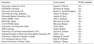
Table 1List of laboratories that participated in the intercomparison. All laboratories measured both methane and nitrous oxide except the U.S. Geological Survey (methane only), UC Santa Barbara (nitrous oxide only), and NOAA PMEL (nitrous oxide from the Pacific Ocean). Also indicated are the 12 laboratories that received the SCOR gas standards of methane and nitrous oxide.
Methods for quantifying dissolved methane and nitrous oxide have evolved and somewhat diverged since the first measurements were made in the 1960s (Craig and Gordon, 1963; Atkinson and Richards, 1967). Some laboratories employ purge-and-trap methods for extracting and concentrating the gases prior to their analysis (e.g., Zhang et al., 2004; Bullister and Wisegarver, 2008; Capelle et al., 2015; Wilson et al., 2017). Others equilibrate a seawater sample with an overlying headspace gas and inject a fixed volume of the gaseous phase into a gas analyzer (e.g., Upstill-Goddard et al., 1996; Walter et al., 2005; Farías et al., 2009). The purge-and-trap technique is typically more sensitive by 1–2 orders of magnitude over headspace equilibrium (Magen et al., 2014; Wilson et al., 2017). However, the purge-and-trap technique requires more time for sample analysis and it is more difficult to automate the injection of samples into the gas analyzer. Headspace equilibrium sampling is most suited for volatile compounds that can be efficiently partitioned into the headspace gas volume from the seawater sample. To compensate for its limited sensitivity, a large volume of seawater can be equilibrated (e.g., Upstill-Goddard et al., 1996). Additional developments for continuous underway surface seawater measurements use equilibrator systems of various designs coupled to a variety of detectors (e.g., Weiss et al., 1992; Butler et al., 1989; Gülzow et al., 2011; Arévalo-Martínez et al., 2013). Determining the level of analytical comparability between different laboratories for discrete samples of methane and nitrous oxide is an important step towards improved comprehensive global assessments. Such intercomparison exercises are critical to determining the spatial and temporal variability of methane and nitrous oxide across the world oceans with confidence, since no single laboratory can single-handedly provide all the required measurements at sufficient resolution. Previous comparative exercises have been conducted for other trace gases, e.g., carbon dioxide, dimethylsulfide, and sulfur hexafluoride (Dickson et al., 2007; Bullister and Tanhua, 2010; Swan et al., 2014), and for trace elements (Cutter, 2013). These exercises confirm the value of the intercomparison concept.
To instigate this process for methane and nitrous oxide, a series of international intercomparison exercises were conducted between 2013 and 2017, under the auspices of Working Group no. 143 of the Scientific Committee on Oceanic Research (SCOR). Discrete seawater samples collected from the subtropical Pacific Ocean and the Baltic Sea were distributed to the participating laboratories (Table 1). The samples were selected to cover a representative range of concentrations across marine locations, from the oligotrophic open ocean to highly productive waters, and in some instances sub-oxic coastal waters. An integral component of the intercomparison exercise was the production and distribution of methane and nitrous oxide gas standards to members of the SCOR Working Group. The intercomparison exercise was conceived and evaluated with the following four questions in mind.
- Q1
What is the agreement between the SCOR gas standards and the “in-house” gas standards used by each laboratory?
- Q2
How do measured values of dissolved methane and nitrous oxide compare across laboratories?
- Q3
Despite the use of different analytical systems, are there general recommendations to reduce uncertainty in the accuracy and precision of methane and nitrous oxide measurements?
- Q4
What are the implications of interlaboratory differences for determining the spatial and temporal variability of methane and nitrous oxide in the oceans?
2.1 Calibration of nitrous oxide and methane using compressed gas standards
Laboratory-based measurements of oceanic methane and nitrous oxide require separation of the dissolved gas from the aqueous phase, with the analysis conducted on the gaseous phase. Calibration of the analytical instrumentation used to quantify the concentration of methane and nitrous oxide is nearly always conducted using compressed gas standards, the specifics of which vary between laboratories. Therefore, the reporting of methane and nitrous oxide datasets ought to be accompanied by a description of the standards used, including their methane and nitrous oxide mole fractions, the declared accuracies, and the composition of their balance or “makeup” gas. For both gases, the highest-accuracy commercially available standards have mole fractions close to current-day atmospheric values. These standards can be obtained from national agencies including the National Oceanic and Atmospheric Administration Global Monitoring Division (NOAA GMD), the National Institute of Metrology China, and the Central Analytical Laboratories of the European Integrated Carbon Observation System Research Infrastructure (ICOS-RI). By comparison, it is more difficult to obtain highly accurate methane and nitrous oxide gas standards with mole fractions exceeding modern-day atmospheric values. This is particularly problematic for nitrous oxide due to the nonlinearity of the widely used electron capture detector (ECD) (Butler and Elkins, 1991).
The absence of a widely available high mole fraction, high-accuracy nitrous oxide gas standard was noted as a primary concern at the outset of the intercomparison exercise. Therefore, a set of high-pressure primary gas standards was prepared for the SCOR Working Group by John Bullister and David Wisegarver at NOAA Pacific Marine and Environmental Laboratory (PMEL). One batch, referred to as the air ratio standard (ARS), had methane and nitrous oxide mole fractions similar to modern air, and the other batch, referred to as the water ratio standard (WRS), had higher methane and nitrous oxide mole fractions for the calibration of high-concentration water samples. These SCOR primary standards were checked for stability over a 12-month period and assigned mole fractions on the same calibration scale, known as “SCOR-2016”. A comparison was conducted with NOAA standards prepared on the SIO98 calibration scale for nitrous oxide and the NOAA04 calibration scale for methane. Based on the comparison with NOAA standards, the uncertainty of the methane and nitrous oxide mole fractions in the ARS and the uncertainty of the methane mole fraction in the WRS were all estimated at <1 %. By contrast, the uncertainty of the nitrous oxide mole fraction in the WRS was estimated at 2 %–3 %. The gas standards were distributed to 12 of the laboratories involved in this study (Table 1). The technical details on the production of the gas standards and their assigned absolute mole fractions are included in Bullister et al. (2016).
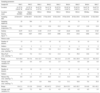
Table 2Pertinent information for each batch of methane and nitrous oxide samples. This includes contextual hydrographic information, median and mean concentrations of methane and nitrous oxide, range, number of outliers, and the overall average coefficient of variation (%).
2.2 Collection of discrete samples of nitrous oxide and methane
Dissolved methane and nitrous oxide samples for the intercomparison exercise were collected from the subtropical Pacific Ocean and the Baltic Sea. Pacific samples were obtained on 28 November 2013 and 24 February 2017 from the Hawai'i Ocean Time-series (HOT) long-term monitoring site, station ALOHA, located at 22.75∘ N, 158.00∘ W. The November 2013 samples are included in Figs. S1 and S2 in the Supplement, but are not discussed in the main Results or Discussion because fewer laboratories were involved in the initial intercomparison, and the results from these samples support the same conclusions obtained with the more recent sample collections. Seawater was collected using Niskin-like bottles designed by John Bullister (NOAA PMEL), which help minimize the contamination of trace gases, in particular chlorofluorocarbons and sulfur hexafluoride (Bullister and Wisegarver, 2008). The bottles were attached to a rosette with a conductivity–temperature–depth (CTD) package. Seawater was collected from two depths: 700 and 25 m, at which the near maximum and minimum water-column concentrations for methane and nitrous oxide at this location can be found. The 25 m samples were always well within the surface mixed layer, which ranged from 100 to 130 m of depth during sampling. Replicate samples were collected from each bottle, with one replicate reserved for analysis at the University of Hawai'i to evaluate variability between sampling bottles. Seawater was dispensed from the Niskin-like bottles using Tygon® tubing into the bottom of borosilicate glass bottles, allowing for the overflow of at least two sample volumes and ensuring the absence of bubbles. Most sample bottles were 240 mL in size and were sealed with no headspace using butyl rubber stoppers and aluminum crimp seals. A few laboratory groups requested smaller crimp-sealed glass bottles ranging from 20–120 mL in volume and two laboratories used 1 L glass bottles, which were closed with a glass stopper and sealed with Apiezon® grease. Seawater samples were collected in quadruplicate for each laboratory. All samples were preserved using saturated mercuric chloride solution (100 µL of saturated mercuric chloride solution per 100 mL of seawater sample) and stored in the dark at room temperature until shipment. The choice of mercuric chloride as the preservative for dissolved methane and nitrous oxide was due to its long history of usage. It is recognized that other preservatives have been proposed (e.g., Magen et al., 2014; Bussmann et al., 2015); however, pending a community-wide evaluation of their effectiveness over a range of microbial assemblages and environmental conditions for both methane and nitrous oxide, it is not evident that they are a superior alternative to mercuric chloride.
Samples from the western Baltic Sea were collected during 15–21 October 2016 onboard the R/V Elisabeth Mann Borgese (Table 2). Since the Baltic Sea consists of different basins with varying concentrations of oxygen beneath permanent haloclines (Schmale et al., 2010), a larger range of water-column methane and nitrous oxide concentrations were accessible for interlaboratory comparison compared to station ALOHA. For all seven Baltic Sea stations, the water column was sampled into an on-deck 1000 L water tank that was subsequently subsampled into discrete sample bottles. At three stations (BAL1, BAL3, and BAL6), the water tank was filled from the shipboard high-throughput underway seawater system. For deeper water-column sampling at the stations BAL2, BAL4, and BAL5, the water tank was filled using a pumping CTD system (Strady et al., 2008) with a flow rate of 6 L min−1 and a total pumping time of approximately 3 h. For the final deep water-column station, BAL7, the pump that supplied the shipboard underway system was lowered to a depth of 21 m to facilitate a shorter pumping time of approximately 20 min. Subsampling the water tank for all samples took approximately 1 h in total and the total sampling volume was less than 100 L. To verify the homogeneity of the seawater during the sampling process, the first and last samples collected from the water tank were analyzed by Newcastle University onboard the research vessel. In contrast to the Pacific Ocean sampling, which predominantly used 240 mL glass vials, each laboratory provided their own preferred vials and stoppers for the Baltic Sea samples. Seawater samples were collected in triplicate for each laboratory. All samples were preserved with 100 µL of saturated mercuric chloride solution per 100 mL of seawater sample, with the exception of samples collected by the U.S. Geological Survey, which analyzed unpreserved samples onboard the research vessel.
2.3 Sample analysis
Each laboratory measured dissolved methane and nitrous oxide slightly differently. A full description of each laboratory's method can be found in Tables S6 and S7 in the Supplement for methane and nitrous oxide, respectively.
The majority of laboratories measured methane and nitrous oxide by equilibrating the seawater sample with an overlying headspace and subsequently injecting a portion of the gaseous phase into the gas analyzer. This method has been conducted since the 1960s when gas chromatography was first used to quantify dissolved hydrocarbons (McAuliffe, 1963). The headspace was created using helium, nitrogen, or high-purity air to displace a portion of the seawater sample within the sample bottle. Alternatively, a subsample of the seawater was transferred to a gastight syringe and the headspace gas subsequently added. The volume of the vessel used to conduct the headspace equilibration ranged from 20 mL borosilicate glass vials to 1 L glass vials and syringes used by Newcastle University and the U.S. Geological Survey, respectively. The dissolved gases equilibrated with the overlying headspace at a controlled temperature for a set period of time that ranged from 20 min to 24 h for the different laboratories. The longer equilibration times are due to overnight equilibrations in water baths. The majority of laboratories enhanced the equilibration process by some initial period of physical agitation. After equilibration, an aliquot of the headspace was transferred into the gas analyzer (GA) by either physical injection, displacement using a brine solution, or injection using a switching valve. Some laboratories incorporated a drying agent and a carbon dioxide scrubber prior to analysis. The gas sample passed through a multi-port injection valve containing a sample loop of known volume, which transferred the gas sample directly onto the analytical column within the oven of the GA. Calibration of the instrument was achieved by passing the gas standards through the injection valve.
The final gas concentrations using the headspace equilibration method were calculated by
where β is the Bunsen solubility of nitrous oxide (Weiss and Price, 1980) or methane (Wiesenburg and Guinasso, 1979) in nmol L−1 atm−1, x is the dry gas mole fraction (ppb) measured in the headspace, P is the atmospheric pressure (atm), Vwp is the volume of water sample (mL), Vhs is the volume (mL) of the created headspace, R is the gas constant (0.08205746 L atm K−1 mol−1), and T is the equilibration temperature in Kelvin (K). An example calculation is provided in Table S8 in the Supplement.
In contrast to the headspace equilibrium method, five laboratories used a purge-and-trap system for methane and/or nitrous oxide analysis (Tables S6 and S7 in the Supplement). These systems were directly coupled to a flame ionization detector (FID) or ECD, with the exception of the University of British Columbia, where a quadrupole mass spectrometer with an electron impact ion source and Faraday cup detector were used (Capelle et al., 2015). The purge-and-trap systems were broadly similar, each transferring the seawater sample to a sparging chamber. Sparging times typically ranged from 5–10 min and the sparge gas was either high-purity helium or high-purity nitrogen. In addition to commercially available gas scrubbers, purification of the sparge gas was achieved by passing it through stainless steel tubing packed with Poropak Q and immersed in liquid nitrogen. This is a recommended precaution to consistently achieve a low blank signal of methane. The elutant gas was dried using Nafion or Drierite and subsequently cryotrapped on a sample loop packed with Porapak Q to aid the retention of methane and nitrous oxide. Cryotrapping was achieved for methane using liquid nitrogen (−195 ∘C) and either liquid nitrogen or cooled ethanol (−70 ∘C) for nitrous oxide. Subsequently, the valve was switched to inject mode and the sample loop was rapidly heated to transfer its contents onto the analytical column. Calibration was achieved by injecting standards via sample loops using multi-port injection valves. The injection of standards upstream of the sparge chamber allowed for calibration of the purge-and-trap gas-handling system, in addition to the GA. Calculation of the gas concentrations using the purge-and-trap method was achieved by the application of the ideal gas law to the standard gas measurements:
where P, R, and T are the same as Eq. (1), V represents the volume of gas injected (L), and n represents moles of gas injected. Rearranging Eq. (2) yields the number of moles of methane or nitrous oxide gas for each sample loop injection of compressed gas standards. These values were used to determine a calibration curve based on the measured peak areas of the injected standards and thereafter derive the number of moles measured for each unknown sample. To calculate concentrations of methane or nitrous oxide in a water sample, the number of moles measured was divided by the volume (L) of seawater sample analyzed. An example calculation is provided in Table S8 in the Supplement.
2.4 Data analysis
The final concentrations of methane and nitrous oxide are reported in nmol kg−1. The analytical precision for each batch of samples obtained by each of the individual laboratories was estimated from the analysis of replicate seawater samples and reported as the coefficient of variation (%). The values reported by each laboratory for all the batches of seawater samples are shown in Tables S1 to S4 in the Supplement. Due to the observed interlaboratory variability, it is likely that the median value of methane and nitrous oxide for each batch of samples does not represent the absolute in situ concentration. As this complicates the analytical accuracy for each laboratory, we instead calculated the percentage difference between the median concentration determined for each set of samples and the mean value reported by an individual laboratory. The presence of outliers was established using the interquartile range (IQR) and by comparing with 1 standard deviation applied to the overall median value.
3.1 Comparison of methane and nitrous oxide gas standards
Six laboratories compared their existing “in-house” standards of methane with the SCOR standards. This was done by calibrating in-house standards and deriving a mixing ratio for the SCOR standards, which were treated as unknowns. Four laboratories reported methane values for either the ARS or WRS within 3 % of their absolute concentration, whereas two laboratories reported an offset of 6 % and 10 % between their in-house standards and the SCOR standards (Table S6 in the Supplement). For those laboratories who measured the SCOR standards to within 3 % or better accuracy, observed offsets in methane concentrations from the overall median cannot be due to the calibration gas.

Figure 1Concentrations of methane measured in nine separate seawater samples collected from the Pacific Ocean (a, b) and the Baltic Sea (c, d, e). The dashed grey line represents the value of methane at atmospheric equilibrium (b). Individual data points are plotted sequentially by increasing value. The same color symbol is used for each laboratory in all plots.
Seven laboratories compared their own in-house standards of nitrous oxide with the prepared SCOR standards. Six laboratories reported values of nitrous oxide for the ARS that were within 3 % of the absolute concentration, with the remaining laboratory reporting an offset of 10 % (Table S7 in the Supplement). The majority of these laboratories (five out of six groups) compared the SCOR ARS with NOAA GMD standards, which have a balance gas of air instead of nitrogen. Some laboratories with analytical systems that incorporated fixed sample loops (e.g., 1 or 2 mL loops housed in a 6-port or 10-port injection valve) had difficulty analyzing the WRS, as the peak areas created by the high mole fraction of the standard exceeded the signal typically measured from in-house standards or acquired by sample analysis by an order of magnitude. The high mole fraction of the WRS was not an issue when multiple sample loops of varying sizes were incorporated into the analytical system, which was the case for purge-and-trap-based designs. For the two laboratories with an in-house standard of comparable mole fraction to the WRS, an offset of 3 % and a >20 % offset were reported.
3.2 Methane concentrations in the intercomparison samples
Overall, median methane concentrations in seawater samples collected from the Pacific Ocean and the Baltic Sea ranged from 0.9 to 60.3 nmol kg−1 (Table 2). Out of 101 reported values, 3 outliers were identified using the IQR criterion and were not included in further analysis. The methane data values for each batch of samples analyzed by each laboratory, including the mean and standard deviation, the number of samples analyzed, and the percent of offset from the overall median value, are reported in Tables S1 and S2 in the Supplement. Analysis conducted by the University of Hawai'i of methane and nitrous oxide from each Niskin-like bottle used in the Pacific Ocean sampling did not reveal any bottle-to-bottle differences. Furthermore, analysis by Newcastle University showed there was no difference between the first and the last set of samples collected from the 1000 L collection used in the Baltic Sea sampling.
The two Pacific Ocean sampling sites had the lowest water-column concentrations of methane (Fig. 1a and b). The PAC1 samples collected from within the mesopelagic zone, where methane concentrations have been reported to be less than 1 nmol kg−1 (Reeburgh, 2007; Wilson et al., 2017), showed a distribution of reported concentrations skewed towards the higher values. For the PAC1 samples, 7 out of 12 laboratories reported values ≤1 nmol kg−1 and the mean coefficient of variation for all laboratories was 11 % (Table 2). In contrast to the mesopelagic samples, the methane concentrations for the near-surface seawater samples (PAC2) were close to atmospheric equilibrium (Fig. 1b). Measured concentrations of methane for PAC2 samples ranged from 1.9 to 3.8 nmol kg−1 and the mean coefficient of variation for all laboratories was 7 %. Similar to the PAC1 samples, PAC2 also had a distribution of data skewed towards the higher concentrations.

Figure 2Deviation from the median methane concentration (reported as absolute values in nmol kg−1) for the seven Baltic Sea samples. The batches of seawater samples: BAL1, BAL3, and BAL6 (a); BAL4, BAL5, and BAL7 (b); BAL2 (c). The shaded grey area indicates values ≤5 % of the median concentration. The color scheme for each laboratory dataset is identical to that used in Fig. 1 and the letters allocated to each dataset are to facilitate cross-referencing in the text. Note that the y axis scale varies between the figures.
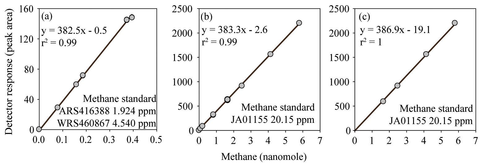
Figure 3FID response to methane fitted with a linear regression calibration. The inclusion (a, b) or exclusion (c) of low methane values causes the calibration slope and intercept to vary. However, the observed variation in the calibration slope does not have a significant effect on the final calculated concentrations of methane. In contrast, variation in the intercept does have an effect on the final concentrations of methane.
Three Baltic Sea sampling sites (BAL1, BAL3, and BAL6) had median methane concentrations that ranged from 4.1 to 5.7 nmol kg−1 (Fig. 1c). The BAL1 samples also showed a skewed distribution of reported values towards higher concentrations, as seen in PAC1 and PAC2 samples. However, this was not evident in BAL3 or BAL6, which had the closest agreement between the reported methane concentrations. For these three sets of Baltic Sea samples, the mean coefficient of variation for all laboratories ranged from 4 % (BAL3) to 9 % (BAL1). The next three Baltic Sea samples (BAL4, BAL5, and BAL7) had methane concentrations that ranged from 18.8 to 35.4 nmol kg−1 (Fig. 1d). These three sets of samples had a normal distribution of data and the closest agreement between the reported concentrations for all of the Pacific Ocean and Baltic Sea samples. Furthermore, for these three sets of samples, the mean coefficient of variation for all laboratories was 4 % (Table 2). The final Baltic Sea sample (BAL2) had the highest concentrations of methane, with a median reported value of 60.3 nmol kg−1 and a large range of values (45.2 to 67.2 nmol kg−1; Fig. 1e). The BAL2 samples had the lowest overall mean coefficient of variation for all laboratories: 2 % (Table 2).
Further analysis of the data was conducted to better comprehend the factors that caused the observed interlaboratory variability in methane measurements. The deviation from median values was calculated for each sample collected from the Baltic Sea (Fig. 2). The Pacific Ocean samples (PAC1 and PAC2) were not included in this analysis due to the skewed distribution of data. There were also some instances in the Baltic Sea samples for which the median concentration might not have realistically represented the absolute in situ methane concentration. This was most likely to have occurred at low concentrations due to the skewed distribution of reported concentrations (e.g., BAL1) or at high concentrations for which there was a large range in reported values (e.g., BAL2). The results revealed that a few laboratories (Datasets D, F, and G) were consistently within or close to 5 % of the median value for all batches of seawater samples (Fig. 2). Some laboratories (e.g., Datasets B, C, and H) had a higher deviation from the median value at higher methane concentrations. Two laboratories (Datasets J and K) had a higher deviation from the median value at lower methane concentrations. Finally, in some cases it was not possible to determine a trend (Datasets A and E) due to the variability.
The reasons behind the trends for each dataset became more apparent when considering the effect of the inclusion or exclusion of low standards in the calibration curve on the resulting derived concentrations (Fig. 3). The FID has a linear response to methane at nanomolar values and therefore a high level of accuracy across a relatively wide range of in situ methane concentrations can be obtained with the correct slope and intercept. To demonstrate this, calibration curves for methane were provided by the University of Hawai'i. These revealed minimal variation in the slope value when calibration points were increased from low mole fractions (Fig. 3a) to higher mole fractions (Fig. 3b). However, the intercept value was sensitive to the range of calibration values used, and this effect was further exacerbated when only the higher calibration points were included (i.e., Fig. 3c). The relevance to final methane concentrations is demonstrated by considering the values reported by the University of Hawai'i for PAC2 samples (Fig. 1b). An almost 30 % increase in final methane concentration occurs from the use of the calibration equation in Fig. 3c compared to Fig. 3a. This derives from a measured peak area for methane of 62 for a sample with a volume of 0.076 L and a seawater density of 1024 kg m−3, yielding a final methane concentration of 2.1 and 2.8 nmol kg−1 using the equations from Fig. 3a and c, respectively. With this understanding on the effect of FID calibration, we consider it likely that the increased deviation from median values at high methane concentrations (Datasets B, C, and H) results from differences in calibration slope between each laboratory. In contrast, the datasets with a higher offset at low methane concentrations (Datasets J and K) could be due to erroneous low standard values causing a skewed intercept. In addition, there may be other factors including sample contamination, which is discussed in Sect. 3.4.
3.3 Nitrous oxide concentrations in the intercomparison samples
Overall, median nitrous oxide concentrations in seawater samples collected from the Pacific Ocean and the Baltic Sea ranged from 3.4 to 42.4 nmol kg−1 (Table 2). Of the 113 reported values, 10 outliers were identified using the IQR criterion and were not included in further analysis. The nitrous oxide data values for each batch of samples analyzed by each laboratory, including the mean and standard deviation, the number of samples analyzed, and the percent of offset from the overall median value are reported in Tables S3 and S4 in the Supplement.
For six sets of seawater samples, BAL1, BAL2, BAL3, BAL6, BAL7, and PAC2, the concentrations of nitrous oxide were close to atmospheric equilibrium. The reported values ranged from 7.7 to 12.7 nmol kg−1 in the Baltic Sea (Fig. 4a) and from 5.9 to 7.6 nmol kg−1 in the Pacific Ocean (Fig. 4b). For the Pacific Ocean near-surface (mixed layer) sampling site (PAC2), the theoretical value of nitrous oxide concentration in equilibrium with the overlying atmosphere is also shown (Fig. 4b). For these six samples with concentrations close to atmospheric equilibrium, the mean coefficient of variation for all laboratories ranged from 3 % (BAL3 and PAC2) to 5 % (BAL1) (Table 2).

Figure 4Concentrations of nitrous oxide measured in nine separate samples from the Baltic Sea and the Pacific Ocean. The dashed grey line represents the value of nitrous oxide at atmospheric equilibrium (b). Individual data points are plotted sequentially by increasing value. The same color symbol is used for each laboratory in all plots.
For the three other sets of samples (BAL4, BAL5, and PAC1), the nitrous oxide concentrations deviated significantly from atmospheric equilibrium (Fig. 4c, d, and e). At one sampling site, BAL4 (Fig. 4c), nitrous oxide was undersaturated with respect to atmospheric equilibrium and reported concentrations ranged from 2.1–5.5 nmol kg−1. As observed in the low-concentration Pacific Ocean methane samples, there was a skewed distribution of the data towards the higher nitrous oxide concentrations. The BAL4 samples also had the highest variability (i.e., lowest precision), with a mean coefficient of variation of 8 % (Table 2). The two remaining samples (PAC1 and BAL5) had much higher concentrations of nitrous oxide, as expected for low-oxygen regions of the water column. In contrast to the samples with near atmospheric equilibrium concentrations of nitrous oxide, there was a low overall agreement between the independent laboratories for PAC1 and BAL5 nitrous oxide concentrations (Fig. 4d, e). At PAC1 and BAL5, nitrous oxide concentrations ranged from 34.3–45.8 nmol kg−1 (Fig. 4d) and 30.1–45.9 nmol kg−1, respectively (Fig. 4e). The mean coefficient of variation for all laboratories was 4 % for BAL5 samples compared to 3 % for PAC1 samples.
The deviation of individual nitrous oxide concentrations from the median value provides insight into the variability associated with their measurements (Fig. 5). The BAL1 dataset was not included in this analysis due to its skewed data distribution, and the high interlaboratory variability for BAL5 indicated that the median value may differ from the absolute nitrous oxide concentration for this sample. For the low-nitrous-oxide Baltic Sea and Pacific Ocean samples (Fig. 5a), the majority of data points were within 5 % of the median values. Furthermore, for the majority of laboratories, the data points for separate seawater samples clustered together, indicating some consistency to the extent they varied from the overall median value. Exceptions to this observation include Datasets E, C, L, and K (Fig. 5a), which demonstrated varying precision and accuracy. At high nitrous oxide concentrations (Fig. 5b), there are fewer data points within 5 % of the median value compared to low nitrous oxide concentrations (Fig. 5a). Therefore, for PAC1 and BAL5 samples, six and seven data points fall within 5 % of the median value, respectively. Furthermore, only three laboratories (Datasets F, G, and K) had data for both Pacific Ocean and Baltic Sea samples within 5 % of the median value. This could have been caused by inconsistent analysis between different batches of samples or by variable sample collection and transportation.

Figure 5Deviation from the median value (reported in absolute units) for nitrous oxide datasets. The batches of samples include BAL1, 2, 3, 6, and 7 (a) and PAC2 and BAL5 (b). The Baltic Sea samples are represented by circles and the Pacific Ocean samples are represented by triangles. The shaded area indicates a deviation ≤5 % from the median value based on a water-column concentration of 11 and 42 nmol kg−1 for (a) and (b), respectively. The color scheme for each laboratory dataset is identical to that used in Fig. 4 and the letters allocated to each dataset are to facilitate cross-referencing in the text. Note the y axis for (a) and (b) are plotted on a different scale.
The likely factors that caused these offsets in nitrous oxide concentrations among laboratories include sample analysis and calibration of the gas analyzers. Calibration of the ECD is nontrivial and at least two prior publications have discussed nitrous oxide calibration issues (Butler and Elkins, 1991; Bange et al., 2001). The laboratories participating in the nitrous oxide intercomparison employed different calibration procedures (Fig. 6). Some used a linear fit and kept their analytical peak areas within a narrow range (Fig. 6a), while others used a stepwise linear fit and therefore used different slopes for low and high nitrous oxide mole fractions (Fig. 6b). Finally, some applied a polynomial curve (Fig. 6c) and sometimes two different polynomial fits for low and high concentrations. The difficulty in calibrating the ECD was evidenced by the deviation from median values as multiple datasets show good precision but consistent offsets at the lowest (Fig. 5a) and highest (Fig. 5b) final concentrations of nitrous oxide.
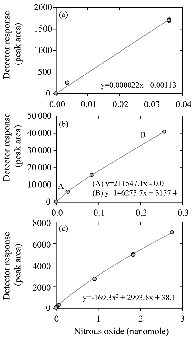
Figure 6Three calibration curves for nitrous oxide measurements using an ECD including linear (a), multilinear (b), and quadratic (c) fits.
3.4 Sample storage and sample bottle size
Because the prolonged storage of samples can influence dissolved gas concentrations, including methane and nitrous oxide, the intercomparison dataset was analyzed for sample storage effects (Table S5 in the Supplement). It should, however, be noted that assessing the effect of storage time on sample integrity was not a formal goal of the intercomparison exercise and replicate samples were not analyzed at repeated intervals by independent laboratories, as would normally be required for a thorough analysis. Nonetheless our results did provide some insights into potential storage-related problems. Most notably, there were indications that an increase in storage time caused increased concentrations and increased variability for methane samples with low concentrations, i.e., PAC1 and PAC2 samples, which had median methane concentrations of 0.9 and 2.3 nmol kg−1, respectively (Fig. 7). In comparison, for samples of nitrous oxide with low concentrations there was no trend of increasing values as observed for samples with low methane concentrations.
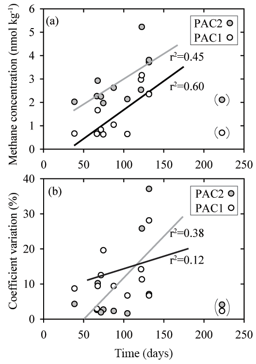
Figure 7Comparison of sample storage times with measured concentrations of methane (a) and coefficient of variation (b) for two sets of seawater samples (PAC1 and PAC2) collected in February 2017. These two sets of seawater samples had the lowest methane concentrations and appear to be influenced by the duration of storage time. The data points enclosed in parentheses were not included in the regression analysis. The PAC1 regression line is black and the PAC2 regression line is grey. All of the storage times are included in the Supplement.
Another variable that differed between laboratories for the intercomparison exercise was the size of sample bottles, which ranged from 25 mL to 1 L for the different laboratories. There was no observed difference between the methane and nitrous oxide values obtained from the various sampling bottles and it was concluded that sampling bottles were not a controlling factor for the observed differences between laboratories. We note, however, the potential for greater air bubble contamination in smaller bottles.
The marine methane and nitrous oxide analytical community is growing. This is reflected in the increasing number of corresponding scientific publications and the resulting development of a global database for methane and nitrous oxide (Bange et al., 2009). Like all Earth observation measurements, there is a need for intercomparison exercises of the type reported here for data quality assurance and for appropriate reporting practices (National Research Council, 1993). To the best of our knowledge, the work presented here is the first formal intercomparison of dissolved methane and nitrous oxide measurements. Based on our results, we discuss the lessons learned and our recommendations moving forward by addressing the four questions that were posed in the Introduction.
4.1 What is the agreement between the SCOR gas standards and the “in-house” gas standards used by each laboratory?
It is typical for laboratories to source some, or all, of their compressed gas standards from commercial suppliers. National agencies, such as NOAA GMD or the National Institute of Metrology China, also provide standards to the scientific community. The national agencies typically offer a lower range in concentrations than commercial suppliers, but their standards tend to have a higher level of accuracy. Of the 12 laboratories participating in the intercomparison, 8 reported using national agency standards, with 7 of them using gases sourced from NOAA GMD. Since the methane and nitrous oxide mole fractions of these national agency standards are equivalent to modern-day atmospheric mixing ratios, they are similar to the SCOR ARS distributed to the majority of laboratories in this study. Laboratories in receipt of the SCOR standards were asked to predict their mole fractions based on those of their own in-house standards. For the majority that conducted this exercise, there was good agreement (<3 % difference) between the NOAA GMD and the SCOR ARS for both methane and nitrous oxide. For three laboratories, a larger offset was observed between the NOAA GMD and the SCOR ARS. There was also a good prediction for the higher-methane-content SCOR WRS, facilitated by the linear response of the FID (Fig. 3). In contrast, the nitrous oxide mole fraction in the SCOR WRS exceeded the typical working range for several laboratories and it was difficult for them to cross-compare with their in-house standards. This reflects an analytical setup that involves on-column injection via a 6-port or 10-port valve with one or two sample loops, respectively. The sample loops have a fixed volume and their inaccessibility makes it difficult to replace them with a smaller loop size. Therefore either dilution of the standard is required, or smaller loops need to be incorporated into the calibration protocol. The two laboratories that compared their in-house standards with the SCOR WRS reported an offset of 3 % and >20 %. This indicates that variability between standards can be an issue for obtaining accurate dissolved concentrations and provides support for the production of a widely available high-concentration nitrous oxide standard. We strongly recommend that all commercially obtained standards are cross-checked against primary standards, such as the SCOR ARS and WRS. This should be conducted at least at the beginning and end of their use to detect any drift that may have occurred during their lifetime. With due diligence and care, the SCOR standards provide the capability for cross-checking personal standards for years to decades (Bullister et al., 2016).
4.2 How do measured values of methane and nitrous oxide compare across laboratories?
4.2.1 Methane
The methane intercomparison highlighted the variability that exists between measurements conducted by independent laboratories. At low methane concentrations, a skewed distribution of methane data was observed, which was particularly evident in PAC1 (Fig. 1a). Potential causes include calibration procedures (Sect. 3.2) and/or sample contamination, which is more prevalent at low concentrations (Sect. 3.4). For some laboratories, the low methane concentrations are close to their detection limit, which is determined by the relatively low sensitivity of the FID and the small number of moles of methane in an introduced headspace equilibrated with seawater. An approximate working detection limit for methane analysis via headspace equilibration is 1 nmol kg−1, although some laboratories improve upon this by having a large aqueous- to gaseous-phase ratio during the equilibration process (e.g., Upstill-Goddard et al., 1996). Depending upon the volume of sample analyzed, purge-and-trap analysis can have a detection limit much lower than 1 nmol kg−1 (e.g., Wilson et al., 2017). Methane measurements in aquatic habitats with methane concentrations near the limit of analytical detection include mesopelagic and high-latitude environments distal from coastal or benthic inputs (e.g., Rehder et al., 1999; Kitidis et al., 2010; Fenwick et al., 2017). Of additional concern is that the skewed distribution of methane concentrations also occurs in samples collected from both the surface ocean (PAC2; Fig. 1b) and coastal environments (BAL1; Fig. 1c). Methane concentrations between 2 and 6 nmol kg−1 are within the detection limit of all participating laboratories. To address this we recommend that laboratories restrict sample storage to the minimum time required to analyze the samples and incorporate internal controls into their sample analysis (Sect. 4.4).
There was an improvement in the overall agreement between the laboratories for samples with higher methane concentrations. However, some of the highest variability between the laboratories was observed at the highest concentrations of methane analyzed (BAL2; Fig. 1e). This high degree of variability resulted in significant uncertainty in the absolute in situ concentration. Methane concentrations of this magnitude and higher are found in coastal environments (Zhang et al., 2004; Jakobs et al., 2014; Borges et al., 2018) and in the water-column associated with seafloor emissions (e.g., Pohlman et al., 2011). These environments are considered vulnerable to climate-induced changes and eutrophication, and therefore it is necessary that independent measurements are conducted to the highest possible accuracy to allow for interlaboratory and inter-habitat comparisons. To address this, we recommend that reference material be produced and distributed between laboratories.
4.2.2 Nitrous oxide
Some of the trends discussed for methane were also evident in the nitrous oxide data. For the samples with the lowest nitrous oxide concentrations a skewed data distribution was observed, as found for methane (Fig. 4c). Such low nitrous oxide concentrations are typical of low-oxygen water-column environments (<10 µmol kg−1). Therefore, the analytical bias towards measuring values higher than the absolute in situ concentrations is particularly pertinent to oceanographers measuring nitrous oxide in oxygen minimum zones and other low-oxygen environments (Naqvi et al., 2010; Farías et al., 2015; Ji et al., 2015). The low concentrations of nitrous oxide still exceed detection limits by at least an order of magnitude for even the less-sensitive headspace method due to the high sensitivity of the ECD. Therefore, the bias towards reporting elevated values for low concentrations of nitrous oxide is related less to analytical sensitivity and is more a consequence of calibration issues. During the intercomparison exercise ECD calibration was identified as a nontrivial issue for all participating laboratories and it deserves continuing attention. In particular, the nonlinearity of the ECD means that low and high nitrous oxide concentrations are more vulnerable to error. This is particularly true if a linear fit is used to calibrate the ECD (Fig. 6a). To circumvent this problem, one laboratory used a stepwise linear function, while other laboratories used a quadratic function. The usefulness of multiple calibration curves for low and high nitrous oxide concentrations was highlighted during the intercomparison exercise, although this necessitates some consideration of the threshold for switching between different calibration curves.
The majority of seawater samples analyzed had nitrous oxide concentrations ranging from 7–11 nmol kg−1 (Fig. 4a, b), which are close to atmospheric equilibrium values, as shown for the Pacific Ocean (Fig. 4b). Collective analysis of these samples gives insight into the precision and accuracy associated with surface-water nitrous oxide analysis (Fig. 5a). This is discussed further in the context of implementing internal controls for methane and nitrous oxide (Sect. 4.4). For samples with the highest nitrous oxide concentrations, i.e., exceeding 30 nmol kg−1, there was high variability between the concentrations reported by the independent laboratories. This was most evident for the BAL5 samples (Fig. 4e) and similar to the variability observed at the highest methane concentrations analyzed (Fig. 1e). It is difficult to assess how much of this variability was specifically due to the differences in calibration practices between the laboratories and the differences in gas standards with high-nitrous-oxide mole fractions, but at least some of it can be attributed to this. These results form the basis for a proposed production of reference material for both trace gases.
4.3 Are there general recommendations to reduce uncertainty in the accuracy and precision of methane and nitrous oxide measurements?
There are several analytical recommendations resulting from this study. The use of highly accurate standards and the appropriate calibration fit is an essential requirement for both headspace equilibration and the purge-and-trap technique. It was shown that both analytical approaches can yield comparable values for methane and nitrous oxide, with the main differences observed at low methane concentrations. At sub-nanomolar methane concentrations, four out of the six laboratories that reported methane concentrations <1 nmol kg−1 used a purge-and-trap analysis.
This study also revealed that sample storage time can be an important factor. Specifically, the results from this study corroborate the findings of Magen et al. (2014), who showed that samples with low concentrations of methane are more susceptible to increased values as a result of contamination. The contamination was most likely due to the release of methane and other hydrocarbons from the septa (Niemann et al., 2015). Since the release of hydrocarbons occurs over a period of time, it is recommended to keep storage time to a minimum and to store samples in the dark. It should be noted that sample integrity can also be compromised due to other factors including inadequate preservation, outgassing, and adsorption of gases onto septa. For all these reasons, it is recommended to conduct an evaluation of sample storage time for the environment that is being sampled.
One useful item that was not included as part of the intercomparison exercise but can help decrease uncertainty in the accuracy and precision of methane and nitrous oxide measurements is internal control measurement. Internal controls represent a self-assessment quality control check to validate the analytical method and quantify the magnitude of uncertainty. Appropriate internal controls for methane and nitrous oxide consist of air-equilibrated seawater samples. Their purpose is to provide checks for methane concentrations ranging from 2–3 nmol kg−1 and for nitrous oxide concentrations ranging from 5–9 nmol kg−1. The air used in the equilibration process could be sourced from the ambient environment, if sufficiently stable, or from a compressed gas cylinder after cross-checking the concentration with the appropriate gas standard. Air-equilibrated samples provide reassurance that the analytical system is providing values within the correct range. Air-equilibrated samples also indicate the certainty associated with calculating the saturation state of the ocean with respect to atmospheric equilibrium. This is particularly relevant when the seawater being sampled is within a few percent of saturation. Finally, these air-equilibrated samples provide an estimate of analytical accuracy, which is infrequently reported for methane or nitrous oxide. At present, only a few studies report the analysis of air-equilibrated seawater alongside water-column samples (Bullister and Wisegarver, 2008; Capelle et al., 2015; Bourbonnais et al., 2017; Wilson et al., 2017). It is likely that wider implementation would facilitate internal assessment of the analytical system. Since the main equipment required is a water bath and an overhead stirrer, the production is not cost prohibitive. A recommendation of this intercomparison exercise is that laboratories routinely use air-equilibrated seawater samples to provide an estimate of analytical accuracy.
In addition to the self-assessments provided by the analysis of air-equilibrated seawater, this study revealed the need for reference seawater to help assess the accuracy of high-concentration methane and nitrous oxide measurements. Reference seawater in this instance refers to batches of dissolved methane and nitrous oxide samples prepared in the laboratory using an equilibrator setup, as used for dissolved inorganic carbon (Dickson et al., 2007). In the absence of plans for additional intercomparison exercises, the provision of reference seawater will allow laboratories to continue evaluating their own measurements. Finally, the lessons learned during the intercomparison exercises will be the basis for a forthcoming good practice guide for dissolved methane and nitrous oxide.
4.4 What are the implications of interlaboratory differences for determining the spatial and temporal variability of methane and nitrous oxide in the oceans?
The key outcome of this study was the identification of differences in methane and nitrous oxide concentrations for the same batch of seawater samples measured by several independent laboratories. Emergent from this is the distinct possibility that any given laboratory will incorrectly report data, thereby increasing uncertainty over the saturation states of both gases. The tendency to overestimate methane concentrations close to atmospheric equilibrium means that marine emissions of methane to the overlying atmosphere will also be overestimated (Bange et al., 1994; Upstill-Goddard and Barnes, 2016). In contrast, for nitrous oxide there does not appear to be either an underestimation or overestimation of concentrations. Consequently, there is generally a lower inherent uncertainty in its surface ocean saturation state, as previously proposed (Law and Ling, 2001; Forster et al., 2009).
The interlaboratory differences highlighted by this study should be viewed in the context of numerous individual efforts to assess temporal and/or spatial trends in methane and nitrous oxide by way of time series observations (Bange et al., 2010; Farías et al., 2015; Wilson et al., 2017; Fenwick and Tortell, 2018), repeat hydrographic survey lines (de la Paz et al., 2017), and single expeditions. While the value of these in integrating the behavior of methane and nitrous oxide into the hydrography and biogeochemistry of local–regional ecosystems is beyond question, their value would be enhanced by the rigorous cross-validation of analytical protocols. Without this, perceived small temporal and/or spatial changes in water-column concentrations in any given region are difficult to verify unless the data all originate from a single laboratory. In addition, the value of a global methane and nitrous oxide database (e.g., Bange et al., 2009) would to some extent be compromised by the uncertainty. Taking due account of the analytical variability between laboratories will clearly be vital to any future assessment of the changing methane and nitrous oxide budgets of the oceans.
Overall, the intercomparison exercise was invaluable to the growing community of ocean scientists interested in understanding the dynamics of dissolved methane and nitrous oxide in the water column. The level of agreement between independent measurements of dissolved concentrations was evaluated in the context of several contributing factors, including sample analysis, standards, calibration procedures, and sample storage time. Importantly, the intercomparison represents a concerted effort from the scientists involved to critically assess the quality of their data and to initiate the steps required for further improvements. Recommendations arising from the intercomparison include routine cross-calibration of working gas standards against primary standards, minimizing sample storage time, incorporating internal controls (air-equilibrated seawater) alongside routine sample analysis, and the future production of reference seawater for methane and nitrous oxide measurements. These efforts will help resolve temporal and spatial variability, which is necessary for constraining methane and nitrous oxide emissions from aquatic ecosystems and for evaluating the processes that govern their production and consumption in the water column.
Data are available in the Supplement.
The supplement related to this article is available online at: https://doi.org/10.5194/bg-15-5891-2018-supplement.
The authors declare that they have no conflict of interest.
Any use of trade names is for descriptive purposes and does not imply endorsement by the U.S. government.
During the final stages of this work, our coauthor John L. Bullister passed away. The intercomparison exercise greatly benefited from John's scientific expertise on dissolved gases. He will be deeply missed by the oceanographic community.
The methane and nitrous oxide intercomparison exercise was conducted as a
Scientific Committee on Ocean Research (SCOR) Working Group, which receives
funding from the U.S. National Science Foundation (OCE-1546580). Pacific
Ocean seawater samples were collected on HOT cruises, which are supported by
the NSF (including the most recent OCE-1260164 to DMK). Baltic Sea seawater
samples were collected during cruise no. 142 of the R/V Elisabeth Mann Borgese, with the ship time provided by the Leibniz Institute for Baltic Sea
Research Warnemünde. We thank Liguo Guo for help with sampling during the
Baltic Sea cruise. The methane and nitrous oxide gas standards were produced
via a Memorandum of Understanding between the University of Hawai'i and
NOAA-PMEL. Funding for the gas standards was provided by the Center for
Microbial Oceanography: Research and Education (C-MORE;
EF0424599 to David M. Karl),
SCOR, the EU FP7 funded Integrated non-CO2 Greenhouse gas Observation
System (InGOS) (grant agreement no. 284274), and NOAA's Climate Program
Office, Climate Observations Division. Additional support was provided by the
Gordon and Betty Moore Foundation no. 3794 (David M. Karl), the Simons Collaboration on
Ocean Processes and Ecology (SCOPE; no. 329108 to David M. Karl), and the Global
Research Laboratory Program (no. 2013K1A1A2A02078278 to David M. Karl) through the
National Research Foundation of Korea (NRF). Alberto V. Borges is a senior research
associate at the FRS-FNRS. Alyson E. Santoro would like to acknowledge NSF OCE-1437310.
Mercedes de la Paz would like to acknowledge the support of the Spanish Ministry of Economy and
Competitiveness (CTM2015-74510-JIN). Laura Farías received financial support from FONDAP
1511009 and FONDECYT no. 1161138.
Edited by: Ji-Hyung Park
Reviewed by: three anonymous referees
Anderson, B., Bartlett, K., Frolking, S., Hayhoe, K., Jenkins, J., and Salas, W.: Methane and nitrous oxide emissions from natural sources, Office of Atmospheric Programs, US EPA, EPA 430-R-10-001, Washington DC, 2010.
Arévalo-Martínez, D. L., Beyer, M., Krumbholz, M., Piller, I., Kock, A., Steinhoff, T., Körtzinger, A., and Bange, H. W.: A new method for continuous measurements of oceanic and atmospheric N2O, CO and CO2: performance of off-axis integrated cavity output spectroscopy (OA-ICOS) coupled to non-dispersive infrared detection (NDIR), Ocean Sci., 9, 1071–1087, https://doi.org/10.5194/os-9-1071-2013, 2013.
Atkinson, L. P. and Richards, F. A.: The occurence and distribution of methane in the marine environment, Deep-Sea Res., 14, 673–684, 1967.
Bange, H. W., Bartell, U. H., Rapsomanikis, S., and Andreae, M. O.: Methane in the Baltic and North Seas and a reassessment of the marine emissions of methane, Global Biogeochem. Cy., 8, 465–480, https://doi.org/10.1029/94GB02181, 1994.
Bange, H. W., Rapsomanikis, S., and Andreae, M. O.: Nitrous oxide cycling in the Arabian Sea, J. Geophys. Res.-Oceans, 106, 1053–1065, 2001.
Bange, H. W., Bell, T. G., Cornejo, M., Freing, A., Uher, G., Upstill-Goddard, R. C., and Zhang G.: MEMENTO: a proposal to develop a database of marine nitrous oxide and methane measurements, Environ. Chem., 6, 195–197, 2009.
Bange, H. W., Bergmann, K., Hansen, H. P., Kock, A., Koppe, R., Malien, F., and Ostrau, C.: Dissolved methane during hypoxic events at the Boknis Eck time series station (Eckernförde Bay, SW Baltic Sea), Biogeosciences, 7, 1279–1284, https://doi.org/10.5194/bg-7-1279-2010, 2010.
Borges, A. V., Speeckaert, G., Champenois, W., Scranton, M. I., and Gypens, N.: Productivity and temperature as drivers of seasonal and spatial variations of dissolved methane in the Southern Bight of the North Sea, Ecosystems, 21, 583–599, https://doi.org/10.1007/s10021-017-0171-7, 2018.
Bourbonnais, A., Letscher, R. T., Bange, H. W., Échevin, V., Larkum, J., Mohn, J., Yoshida, N., and Altabet, M. A.: N2O production and consumption from stable isotopic and concentration data in the Peruvian coastal upwelling system, Global Biogeochem. Cy., 31, 678–698, https://doi.org/10.1002/2016GB005567, 2017.
Bullister, J. L. and Tanhua, T.: Sampling and measurement of chlorofluorocarbons and sulfur hexafluoride in seawater, IOCCP Report No. 14 ICPO Publication Series No. 134, Version 1, available at: http://www.go-ship.org/HydroMan.html (last access: September 2018), 2010.
Bullister, J. L. and Wisegarver, D. P.: The shipboard analysis of trace levels of sulfur hexafluoride, chlorofluorocarbon-11 and chlorofluorocarbon-12 in seawater, Deep-Sea Res., 55, 1063–1074, 2008.
Bullister, J. L., Wisegarver, D. P., and Wilson, S. T.: The production of methane and nitrous oxide gas standards for Scientific Committee on Ocean Research (SCOR) Working Group #143, available at: http://udspace.udel.edu/handle/19716/23288 (last access: September 2018), 2016.
Bussmann, I., Matousu, A., Osudar, R., and Mau, S.: Assessment of the radio 3H-CH4 tracer technique to measure aerobic methane oxidation in the water column, Limnol. Oceanogr.-Meth., 13, 312–327, 2015.
Butler, J. H. and Elkins, J. W.: An automated technique for the measurement of dissolved N2O in natural waters, Mar. Chem., 34, 47–61, 1991.
Butler, J. H., Elkins, J. W., Thompson, T. M., and Egan, K. B.: Tropospheric and dissolved N2O of the west Pacific and east Indian Oceans during the El Niño Southern Oscillation event of 1987, J. Geophys. Res., 94, 14865–14877, 1989.
Capelle, D. W., Dacey, J. W., and Tortell, P. D.: An automated, high through-put method for accurate and precise measurements of dissolved nitrous oxide and methane concentrations in natural waters, Limnol. Oceanogr.-Meth., 13, 345–355, 2015.
Ciais, P., Dolman, A. J., Bombelli, A., Duren, R., Peregon, A., Rayner, P. J., Miller, C., Gobron, N., Kinderman, G., Marland, G., Gruber, N., Chevallier, F., Andres, R. J., Balsamo, G., Bopp, L., Bréon, F.-M., Broquet, G., Dargaville, R., Battin, T. J., Borges, A., Bovensmann, H., Buchwitz, M., Butler, J., Canadell, J. G., Cook, R. B., DeFries, R., Engelen, R., Gurney, K. R., Heinze, C., Heimann, M., Held, A., Henry, M., Law, B., Luyssaert, S., Miller, J., Moriyama, T., Moulin, C., Myneni, R. B., Nussli, C., Obersteiner, M., Ojima, D., Pan, Y., Paris, J.-D., Piao, S. L., Poulter, B., Plummer, S., Quegan, S., Raymond, P., Reichstein, M., Rivier, L., Sabine, C., Schimel, D., Tarasova, O., Valentini, R., Wang, R., van der Werf, G., Wickland, D., Williams, M., and Zehner, C.: Current systematic carbon-cycle observations and the need for implementing a policy-relevant carbon observing system, Biogeosciences, 11, 3547–3602, https://doi.org/10.5194/bg-11-3547-2014, 2014.
Craig, H. and Gordon, L. I.: Nitrous oxide in the ocean and the marine atmosphere, Geochim. Cosmochim. Ac., 27, 949–955, 1963.
Cutter, G. A.: Intercalibration in chemical oceanography – getting the right number, Limnol. Oceanogr.-Meth., 11, 418–424, 2013.
de la Paz, M., García-Ibáñez, M. I., Steinfeldt, R., Ríos, A. F., and Pérez, F. F.: Ventilation versus biology: What is the controlling mechanism of nitrous oxide distribution in the North Atlantic?, Global Biogeochem. Cy., 31, 745–760, https://doi.org/10.1002/2016GB005507, 2017.
Dickson, A. G., Sabine, C. L., and Christian, J. R.: Guide to best practices for ocean CO2 measurements, PICES Special Publication 3, North Pacific Marine Science Organization, Canada, 2007.
Farías, L., Castro-González, M., Cornejo, M., Charpentier, J., Faúndez, J., Boontanon, N., and Yoshida, N.: Denitrification and nitrous oxide cycling within the upper oxycline of the eastern tropical South Pacific oxygen minimum zone, Limnol. Oceanogr., 54, 132–144, 2009.
Farías, L., Besoain, V., and García-Loyola, S.: Presence of nitrous oxide hotspots in the coastal upwelling area off central Chile: an analysis of temporal variability based on ten years of a biogeochemical time series, Environ. Res. Lett., 10, 044017, https://doi.org/10.1088/1748-9326/10/4/044017, 2015.
Fenwick, L. and Tortell, P. D.: Methane and nitrous oxide distributions in coastal and open ocean waters of the Northeast Subarctic Pacific during 2015–2016, Mar. Chem., 200, 45–56, 2018.
Fenwick, L., Capelle, D., Damm, E., Zimmermann, S., Williams, W. J., Vagle, S., and Tortell, P. D.: Methane and nitrous oxide distributions across the North American Arctic Ocean during summer, 2015, J. Geophys. Res.-Oceans, 122, 390–412, https://doi.org/10.1002/2016JC012493, 2017.
Forster, G., Upstill-Goddard, R. C., Gist, N., Robinson, C., Uher, G., and Woodward, E. M. S.: Nitrous oxide and methane in the Atlantic Ocean between 50∘ N and 52∘ S: latitudinal distribution and sea-to-air flux, Deep-Sea Res., 56, 964–976, 2009.
Freing, A., Wallace, D. W. R., and Bange, H. W.: Global oceanic production of nitrous oxide, Philos. T. R. Soc. B, 367, 1245–1255, 2012.
Gülzow, W., Rehder, G., Schneider, B., Schneider, J., Deimling, V., and Sadkowiak, B.: A new method for continuous measurement of methane and carbon dioxide in surface waters using off-axis integrated cavity output spectroscopy (ICOS): An example from the Baltic Sea, Limnol. Oceanogr.-Meth., 9, 176–184, 2011.
Jakobs, G., Holterman, P., Berndmeyer, C., Rehder, G., Blumenberg, M., Jost, G., Nausch, G., and Schmale, O.: Seasonal and spatial methane dynamics in the water column of the central Baltic Sea (GotlandSea), Cont. Shelf Res., 91, 12–25, 2014.
Ji, Q., Babbin, A. R., Jayakumar, A., Oleynik, S., and Ward, B. B.: Nitrous oxide production by nitrification and denitrification in the Eastern Tropical South Pacific oxygen minimum zone, Geophys. Res. Lett., 42, 10755–10764, https://doi.org/10.1002/2015GL066853, 2015.
Kitidis, A., Upstill-Goddard, R. C., and Anderson, L. G.: Methane and nitrous oxide in surface water along the North-West Passage, Arctic Ocean, Mar. Chem., 121, 80–86, 2010.
Law, C. S. and Ling, R. D.: Nitrous oxide flux and response to increased iron availability in the Antarctic Circumpolar Current, Deep-Sea Res., 48, 2509–2527, 2001.
Magen, C., Lapham, L. L., Pohlman, J. W., Marshall, K., Bosman, S., Casso, M., and Chanton, J. P.: A simple headspace equilibration method for measuring dissolved methane, Limnol. Oceanogr.-Meth., 12, 637–650, 2014.
McAuliffe, C.: Solubility on water of C1–C9 hydrocarbons, Nature, 200, 1092–1093, 1963.
Myhre, G., Shindell, D., Bréon, F.-M., Collins, W., Fuglestvedt, J., Huang, J., Koch, D., Lamarque, J.-F., Lee, D., Mendoza, B., Nakajima, T., Robock, A., Stephens, G., Takemura, T., and Zhang, H.: Anthropogenic and Natural Radiative Forcing, in: Climate Change 2013: The Physical Science Basis. Contribution of Working Group I to the Fifth Assessment Report of the Intergovernmental Panel on Climate Change, edited by: Stocker, T. F., Qin, D., Plattner, G.-K., Tignor, M., Allen, S. K., Boschung, J., Nauels, A., Xia, Y., Bex, V., and Midgley, P. M., Cambridge University Press, Cambridge, UK and New York, NY, USA, 2013.
Naqvi, S. W. A., Bange, H. W., Farías, L., Monteiro, P. M. S., Scranton, M. I., and Zhang, J.: Marine hypoxia/anoxia as a source of CH4 and N2O, Biogeosciences, 7, 2159–2190, https://doi.org/10.5194/bg-7-2159-2010, 2010.
National Research Council: Applications of analytical chemistry to oceanic carbon cycle studies, National Academy Press, Washington DC, 1993.
Nevison, C. D., Weiss, R. F., and Erickson, D. J.: Global oceanic emissions of nitrous oxide, J. Geophys. Res., 100, 15809–15820, https://doi.org/10.1029/95JC00684, 1995.
Niemann, H., Steinle, L., Blees, J., Bussmann, I., Treude, T., Krause, S., Elvert, M., and Lehmann, M. F.: Toxic effects of lab-grade butyl rubber stoppers on aerobic methane oxidation, Limnol. Oceanogr.-Meth., 13, 40–52, 2015.
Pohlman, J. W., Bauer, J. E., Waite, W. F., Osburn, C. L., and Chapman, N. R.: Methane hydrate-bearing seeps as a source of aged dissolved organic carbon to the oceans, Nat. Geosci., 4, 37–41, 2011.
Reeburgh, W. S.: Oceanic methane biogeochemistry, Chem. Rev., 107, 486–513, https://doi.org/10.1021/cr050362v, 2007.
Rehder, G., Keir, R. S., Suess, E., and Rhein, M.: Methane in the northern Atlantic controlled by microbial oxidation and atmospheric history, Geophys. Res. Lett., 26, 587–590, https://doi.org/10.1029/1999GL900049, 1999.
Schmale, O., Schneider von Deimling, J., Gülzow, W., Nausch, G., Waniek, J. J., and Rehder, G.: Distribution of methane in the water column of the Baltic Sea, Geophys. Res. Lett., 37, L12604, https://doi.org/10.1029/2010GL043115, 2010.
Strady, E., Pohl, C., Yakushev, E. V., Krügera, S., and Hennings, U.: PUMP–CTD-System for trace metal sampling with a high vertical resolution. A test in the Gotland Basin, Baltic Sea, Chemosphere, 70, 1309–1319, 2008.
Swan, H. B., Armishaw, P., Iavetz, R., Alamgir, M., Davies, S. R., Bell, T. G., and Jones, G. B.: An interlaboratory comparison for the quantification of aqueous dimethylsulfide, Limnol. Oceanogr.-Meth., 12, 784–794, 2014.
Upstill-Goddard, R. C. and Barnes, J.: Methane emissions from UK estuaries: Re-evaluating the estuarine source of tropospheric methane from Europe, Mar. Chem., 180, 14–23, 2016.
Upstill-Goddard, R. C., Rees, A. P., and Owens, N. J. P.: Simultaneous high-precision measurements of methane and nitrous oxide in water and seawater by single phase equilibration gas chromatography, Deep-Sea Res., 43, 1669–1682, 1996.
Walter, S., Peeken, I., Lochte, K., Webb, A., and Bange, H. W.: Nitrous oxide measurements during EIFEX, the European Iron Fertilization Experiment in the subpolar South Atlantic Ocean, Geophys. Res. Lett., 32, L23613, https://doi.org/10.1029/2005GL024619, 2005.
Weiss, R. F. and Price, B. A.: Nitrous oxide solubility in water and seawater, Mar. Chem., 8, 347–359, https://doi.org/10.1016/0304-4203(80)90024-9, 1980.
Weiss, R. F., Van Woy, F. A., and Salameh, P. K.: Surface water and atmospheric carbon dioxide and nitrous oxide observation by shipboard automated gas chromatography: Results from expeditions between 1977 and 1990, Scripps Institution of oceanography Reference 92-11, ORNL/CDIAC-59, NDP-044, Carbon Dioxide Information Analysis Center, Oak Ridge National Laboratory, Tennessee, 1992.
Wiesenburg, D. A. and Guinasso, N. L.: Equilibrium solubilities of methane, carbon monoxide and hydrogen in water and seawater, J. Chem. Eng. Data, 24, 354–360, https://doi.org/10.1021/je60083a006, 1979.
Wilson, S. T., Ferrón, S., and Karl, D. M.: Interannual variability of methane and nitrous oxide in the North Pacific Subtropical Gyre, Geophys. Res. Lett., 44, 9885–9892, https://doi.org/10.1002/2017GL074458, 2017.
Zhang, G. L., Zhang, J., Kang, Y. B., and Liu, S. M.: Distributions and fluxes of methane in the East China Sea and the Yellow Sea in spring, J. Geophys. Res., 109, C07011, https://doi.org/10.1029/2004JC002268, 2004.