the Creative Commons Attribution 4.0 License.
the Creative Commons Attribution 4.0 License.
 | 04 Sep 2018
Multi-year particle fluxes in Kongsfjorden, Svalbard
Alessandra D'Angelo
Federico Giglio
Stefano Miserocchi
Anna Sanchez-Vidal
Stefano Aliani
Tommaso Tesi
Angelo Viola
Mauro Mazzola
Leonardo Langone
High-latitude regions are warming faster than other areas due to reduction of snow cover and sea ice loss and changes in atmospheric and ocean circulation. The combination of these processes, collectively known as polar amplification, provides an extraordinary opportunity to document the ongoing thermal destabilisation of the terrestrial cryosphere and the release of land-derived material into the aquatic environment. This study presents a 6-year time series (2010–2016) of physical parameters and particle fluxes collected by an oceanographic mooring in Kongsfjorden (Spitsbergen, Svalbard). In recent decades, Kongsfjorden has been experiencing rapid loss of sea ice coverage and retreat of local glaciers as a result of the progressive increase in ocean and air temperatures. The overarching goal of this study was to continuously monitor the inner fjord particle sinking and to understand to what extent the temporal evolution of particulate fluxes was linked to the progressive changes in both Atlantic and freshwater input. Our data show high peaks of settling particles during warm seasons, in terms of both organic and inorganic matter. The different sources of suspended particles were described as a mixing of glacier carbonate, glacier siliciclastic and autochthonous marine input. The glacier releasing sediments into the fjord was the predominant source, while the sediment input by rivers was reduced at the mooring site. Our time series showed that the seasonal sunlight exerted first-order control on the particulate fluxes in the inner fjord. The marine fraction peaked when the solar radiation was at a maximum in May–June while the land-derived fluxes exhibited a 1–2-month lag consistent with the maximum air temperature and glacier melting. The inter-annual time-weighted total mass fluxes varied by 2 orders of magnitude over time, with relatively higher values in 2011, 2013, and 2015. Our results suggest that the land-derived input will remarkably increase over time in a warming scenario. Further studies are therefore needed to understand the future response of the Kongsfjorden ecosystem alterations with respect to the enhanced release of glacier-derived material.


There is ample evidence collected over the last decades that the atmosphere and ocean have warmed, the amounts of snow and ice have diminished, and sea level has risen (IPCC, 2014). Global climate change is amplified in the Arctic by several positive feedbacks, including ice and snow melting that decreases surface albedo and atmospheric stability that traps temperature anomalies near the surface layers (Overpeck et al., 1997).
The physical drivers for the changes attributed to anthropogenic climate change include the increased penetration of warm Atlantic and Pacific water into the Arctic Ocean, increased seawater temperature, reduced cover of sea ice, and increased submarine irradiance (Wassmann et al., 2011). As a result, the temperature in high latitudes is increasing at a rate of 2 to 3 times the global average temperature (ACIA, 2004). Arctic fjord systems will likely be particularly vulnerable to human-induced climate change.
To better understand how the thermal destabilisation of Arctic fjords will occur over time, it is important to establish the current knowledge for these sites. This requires the acquisition of time series for climate-sensitive parameters (Svendsen et al., 2002). Our research is part of the ARCA project (ARctic present Climate change and pAst extreme events), which aimed to develop a conceptual model of the mechanism(s) behind the release of large volumes of cold and fresh water from the melting of ice caps, investigating this complex system from both a palaeoclimatic and modern air–sea–ice interaction process point of view.
Kongsfjorden is largely influenced by the polythermal tidewater glaciers Blomstrandbreen and Conwaybreen, as well as Kongsbreen, Kronebreen, and Kongsvegen (Blaszczyk et al., 2009; Dowdeswell and Forsberg, 1992; Hagen, 1993; Howe et al., 2003; Liestøl, 1988; MacLachlan et al., 2010; Sundfjord et al., 2017; Svendsen et al., 2002). The freshwater outflow from tidewater glaciers plays a double role in the biogeochemistry of the fjord, by favouring the stratification of water masses in the coastal zone during the summer melting season (Harms et al., 2007; Rajagopalan, 2012; Svendsen et al., 2002; Trusel et al., 2010), and the settling of the suspended particulate matter to the bottom, through flocculation (Meslard et al., 2018).
Using an automatic sediment trap moored in the inner Kongsfjorden, 6 years of continuous data (2010–2016) have been collected. The mooring, also equipped with current meters and salinity and temperature sensors, is located between the glaciers termini and the sill, receiving the influence from meltwater from the glacier as well as the Atlantic Water (AW) intrusion through the southern fjord (Cottier et al., 2005; Svendsen et al., 2002).
In order to describe the downward particle fluxes of biogenic and glacier-derived material, geochemical data of sinking particles were combined with the time series of physical environmental data measured in the inner fjord. Our overarching goal was to observe the trend in particulate fluxes over time and to constrain the nature of sinking particles to test to what extent the composition of the trapped material is affected by climate-sensitive aspects (e.g. precipitation, glacier retreat, air and water temperature, water column mixing). In particular, by combining physical and biological parameters, we tested whether the magnitude and composition of particle fluxes in the inner fjord are experiencing changes caused by the global change, and which could be the long-term effects on the biogeochemical cycles.
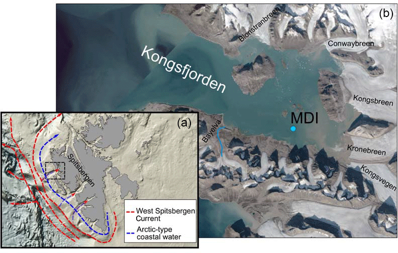
Figure 1(a) Map of Svalbard with a simplified scheme of the main current circulation along the western Spitsbergen region. The light blue line shows the Arctic-type coastal water and the northward red arrow represents the warm West Spitsbergen Current (WSC). (b) Map of Kongsfjorden (area of study). The cyan point shows the Mooring Dirigibile Italia (MDI) site. MDI is located at 100 m of water depth, at the distance of 1.7 km from the southern coast, between the Kronebreen front (7 km far) and the sill. Positions of the Bayelva River and of the main glacier fronts are also shown.
Svalbard is an Arctic archipelago located between 76–81∘ N and 10–34∘ E and surrounded by the Arctic Ocean in the north, the Greenland Sea to the west, and the Barents Sea to the east and south. Spitsbergen is the largest island of the archipelago (Fig. 1a). Kongsfjorden is a glacially eroded fjord, elongated in the SE–NW direction, located along the west coast of Spitsbergen. It is 27 km long, varying in width from 4 km at its head to 10 km at its mouth (Svendsen et al., 2002). The inner part of Kongsfjorden is surrounded by a glacier-dominated coast with five tidewater glaciers: Blomstrandbreen and Conwaybreen, Kongsbreen (north and south), Kronebreen, and Kongsvegen (Blaszczyk et al., 2009; Dowdeswell and Forsberg, 1992; Howe et al., 2003; Liestøl, 1988; MacLachlan et al., 2010; Svendsen et al., 2002) (Fig. 1b). The Fram Strait (Fig. 1a), positioned between northeastern Greenland and the Svalbard archipelago, is the sole conduit conveying warm anomalies from the northern Atlantic to the Arctic Ocean (Beszczynska-Möller et al., 2012). In this deep strait, the upper part of the AW becomes less saline due to the melting sea ice and the mixing with fresh surface water of Arctic origin. This allows the AW to preserve its warm core, losing less heat to the atmosphere (Beszczynska-Möller et al., 2012). The Atlantic warm core (5 ∘C and salinity up to 35 ∘C), in the form of the West Spitsbergen Current (WSC), intrudes into Kongsfjorden, passes the threshold moraine in front of glaciers close to Lovénøyane, and reaches the inner part of the fjord, where it comes into contact with the glacier front (Kongsvegen, Kronebreen, and Kongsbreen termini) (Fig. 1b). This process modifies the WSC characteristics, producing the Transformed Atlantic Water (TAW, 1–3 ∘C) (Aliani et al., 2016; Cottier et al., 2005; Svendsen et al., 2002). Recent changes in the relative inflow of Atlantic and Arctic waters have resulted in significant variability in environmental conditions along the western Spitsbergen shelf (Majewski et al., 2009). In recent years (1997–2010), the AW displayed variability in temperature and transport at the entrance to the Arctic Ocean, exhibiting temperature anomalies of around +2 ∘C (Beszczynska-Möller et al., 2012). This warming has enhanced meltwater fluxes from Svalbard glaciers, influencing fjord hydrology, sea ice conditions, and local biota. Physical, chemical, and biological processes are influenced or constrained by the local quantities and geochemical qualities of freshwater. These include stratification and vertical mixing, ocean heat flux, nutrient supply, primary production, ocean acidification, and biogeochemical cycling (Carmack et al., 2016).
3.1 Time series data collection
A 6-year (September 2010 to May 2016) data set from the Mooring Dirigibile Italia (MDI) deployed in Kongsfjorden (Svalbard) is presented. MDI was installed in the inner fjord at ∼100 m of depth, at the distance of 1.7 km from the southern coast, between the Kronebreen front (7 km from the southern coast) and the sill (Fig. 1). The best site to deploy the long-term data collection equipment was selected after a bathymetric and high-resolution seismic survey at GPS position 78∘55′ N–12∘15′ E. The site is a compromise among properties of the water passing across the strait, the bottom depth, and the modern sediment accumulation rate. The permanent mooring MDI was first deployed in September 2010 and then serviced at annual frequency. It was equipped with a time series Technicap sediment trap (12 receiving cups, model PPS4/3, 0.05 m2 collection area) at ∼20 m above the sea bottom. To prevent organic degradation during deployment, trap sample cups were filled with filtered seawater containing a 5 % formaldehyde buffered solution. The interval of rotation of the sediment trap was variable between 8 and 90 days. The shorter sampling periods correspond to the summer season in which a greater variability in biological and physical–chemical conditions was expected, while the rotation intervals were longer in winter. All programmed samples were recovered, except between 3 August and 11 September 2014 due to a rotation failure. The mooring had a slightly different configuration in different years (Fig. A1).
The sediment trap was typically coupled with a temperature and conductivity recorder (SBE16 SeaCAT), and a single-point current meter (Teledyne RD Instruments Doppler volume sampler, DVS). From mid-2015, the current meter was substituted by an upward acoustic Doppler current profiler (ADCP) (Teledyne RD Instruments Sentinel V100, 300 kHz) in order to obtain water current velocities over a range of depths that encompass the entire water column and, hopefully, also the passage of icebergs or pack ice. To monitor the mid-water characteristics, a single-point current meter with a temperature sensor (Nortek Aquadopp) was tethered at ∼35 m of depth. Additional high-precision thermometers (SBE56) were assembled at nominal depths of 54 and 62 m starting from September 2012 and May 2013, respectively (Fig. A1).
For safety purposes against the passage of icebergs and sea ice, the uppermost buoy was kept submerged; thus no information is available for surface water characteristics and dynamics. Conductivity–temperature–depth (CTD) surveys were performed each summer during the mooring servicing by using a SBE19 probe, providing additional information on the hydrological features in the inner fjord. The accuracy of the individual current speed and direction measurements is ±1 cm s−1 and ±5∘, respectively. The accuracy of SBE16 SeaCAT and SBE56 sensors was checked against CTD casts before and after deployments. Values of solar radiation, wind speed, and direction were obtained from the Amundsen-Nobile Climate Change Tower (CCT) data set (Mazzola et al., 2016) while precipitation values were obtained from the eKlima archive from the Norwegian Meteorological Institute (http://sharki.oslo.dnmi.no, last access: 24 August 2018). The water temperature and salinity and current speed and direction, together with the meteorological and radiation parameters, were measured or averaged at 30 min intervals. Hydrographic and current meter data sets are substantially complete with only a few data gaps of the mid-water current meter (August 2011, May–August 2012, and April–June 2015; Fig. A1), following battery exhaustion.
3.2 Trap sample treatment and analytical methods
Samples recovered from the sediment trap were stored in the dark at 4 ∘C until they were processed at the National Research Council – Institute of Marine Sciences (CNR-ISMAR) in Bologna, Italy, following the method of Chiarini et al. (2014). The organisms classified as swimmers observed in sediment trap samples were removed to avoid an overestimation of the organic content of particle flux and to reduce the bias in sediment flux analysis (Karl and Knauer, 1989). Mineral grains were also removed and considered ice-rafted detritus (IRD), deposited from iceberg melting. The amount of IRD was calculated as flux:
Samples were split into subsamples using a high-precision Perimatic Premier pump dispenser coupled with a robotic XY module to automate the splitting. At least two subsamples (100 mL each) for total mass flux (TMF) determination were filtered through pre-weighed 0.45 µm filter with a mixed cellulose ester membrane, rinsed with distilled water and dried at 50 ∘C for 24 h, then weighed. The total weight of the trapped sediment was converted to flux according to each sample duration and to the trap collection area:
The remaining aliquots were centrifuged for 10 min at 3000 rpm; the excess water was then removed and the tube rinsed with demineralised water to remove any remaining salt or formalin from the sediment. Samples were then centrifuged again at 3000 rpm for 10 min. Finally, excess liquid was removed and the sample freeze-dried. Samples were gently ground to obtain a homogeneous powder (Chiarini et al., 2014) for further chemical analysis. We determined the contents of total carbon (TC), organic carbon (OC), and total nitrogen (TN) and the stable isotope compositions using a Finnigan Delta Plus XP mass spectrometer directly coupled to a Thermo Fisher Scientific FLASH 2000 IRMS element analyser via a ConFlo III interface for continuous flow measurements (Kristensen and Andersen, 1987; Tesi et al., 2007; Verardo et al., 1990). OC contents and stable isotopes were measured on freeze-dried samples after CaCO3 removal with an acid treatment (HCl, 1.5 M). Organic matter (OM) content was estimated as twice the OC content. Carbonate content was calculated assuming all inorganic carbon (% TC − % OC) was in the form of CaCO3 and using the molecular mass ratio 100∕12. The average standard deviation of each measurement, determined by replicate analyses of the same sample, was ±0.07 % for OC and ±0.009 % for TN. Isotopic composition of organic carbon is presented in the conventional δ notation and reported as parts per thousand (‰):
Uncertainties were lower than ±0.05 ‰, as determined from
routine replicate measurements of the reference sample IAEA-CH7
(polyethylene, −32.15 ‰ vs. Vienna Peedee Belemnite, VPDB). Errors for replicate analyses
of the standards were ±0.2 ‰. Biogenic silica (SiO2
0.4H2O) content was analysed using a two-step 2.5 h extraction of 20 mg
of freeze-dried sample with a 0.5 M Na2CO3 solution at 85 ∘C
followed by the measurement of dissolved Si and Al contents in both leachates
with a Perkin Elmer Optima 3200RL inductively coupled plasma optical emission
spectrometer (ICP-OES) at the University of Barcelona. The Si content of the
first leachate was corrected by the Si∕Al ratio of the second one in
order to correct for the excess Si dissolved from aluminosilicates
(Fabres et al., 2002; Kamatani and Oku, 2000; Ragueneau et al., 2005). Biogenic silica was
transformed to opal by multiplying by 2.4 (Mortlock and Froelich, 1989). As the total
composition of a sample is the sum of biogenic and lithogenic components, the
percentage of lithogenic material was obtained assuming the following
relationship:
% lithogenic = 100 − (% OM + % CaCO3 + % opal).
3.3 Principal component analysis (PCA)
A multivariate analysis (PCA) was carried out using the vegan (v. 2.4-2) package in R. The PCA was applied to the transformed data set standardised to a mean of 0 and standard deviation of 1 to visualise intern-specific differences and correlations. Environmental variables were tested for skewness (due to strong seasonal gradients), and heavily left or right skewed data were log transformed log(x+1) to stabilise variance (all data excluding solar radiation, salinity, and air and water temperature). The variables used for the PCA were total mass flux (Mass Flux), organic carbon content (OC), δ13C (C13), inorganic carbon content (IC), opal content (Opal), atmospheric temperature (AirT), solar radiation (Rad), rain precipitation (Precip), wind speed and direction (WindSpeed, WindDir), bottom water salinity (Sal), and bottom water temperature (WatT). The δ13C data were transformed as log(x+26) to ensure positive values. A Spearman's rank correlation matrix was carried out on the data sets to see which could be combined. Missing values for air temperature (n=8) and precipitation (n=6) were calculated based on monthly averages from the rest of the time series. Environmental data were normalised to a mean of 0 and standard deviation of 1 before analysis. Euclidean distances were used to determine spatial ranges within these data.
The current paper focuses on the time series of downward particle fluxes in the inner Kongsfjorden. The environmental variables discussed in the text (i.e. meteorological and oceanographic variables) are included in the discussion although a complete analysis of these parameters will be shown elsewhere (Aliani et al., 2018).
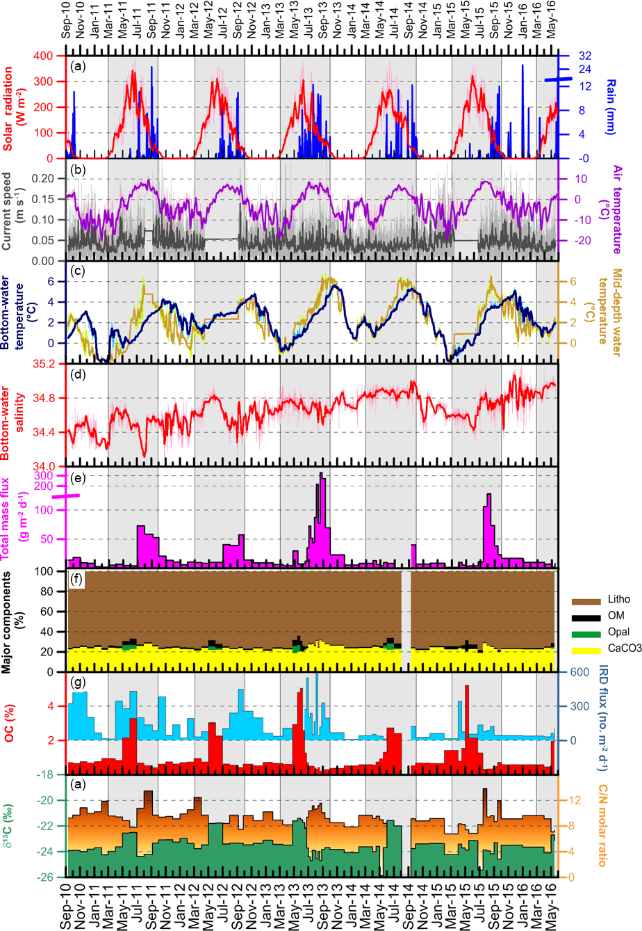
Figure 2Time series of atmospheric and marine parameters recorded in Kongsfjorden between September 2010 and June 2016: (a) solar radiation and rain precipitation, (b) air temperature and mid-water current speed, (c) intermediate and near-bottom water temperature, (d) salinity at the near bottom, (e) total mass flux (TMF) particle fluxes, (f) particle composition, (g) contents of OC and IRD, and (h) C∕N molar ratio and δ13C values measured on the organic fraction. Light grey bands depict the polar day of each year, characterized by enhanced solar radiation. Parameters with high-frequency temporal oscillations (solar radiation, air and water temperatures, salinity, current speed) were plotted with a superimposed week-running average (heavy lines).
4.1 Solar radiation
The solar radiation exhibited a clear seasonal trend, with high values in spring and summer, and near-zero values from November to January, i.e. during the polar night, as expected due to the location of the fjord (Fig. 2a). Monthly means show higher values from May to July, ranging from about 150 to about 270 W m−2, depending on the year. On an annual basis, the year with more insolation (2015) exceeds that with the lowest insolation (2013) by about 13 % (84 to 74 W m−2 are the yearly means) since those values are associated with the cloudiness conditions and influence snow and ice melt. Regarding the seasons, summers presented extreme values equal to 150 W m−2 (2013) and 192 W m−2 (2011), spring values ranging from 117 W m−2 (2016) to 135 W m−2 (2012), and autumn values from 9 W m−2 (2014) to 17 W m−2 (2010).
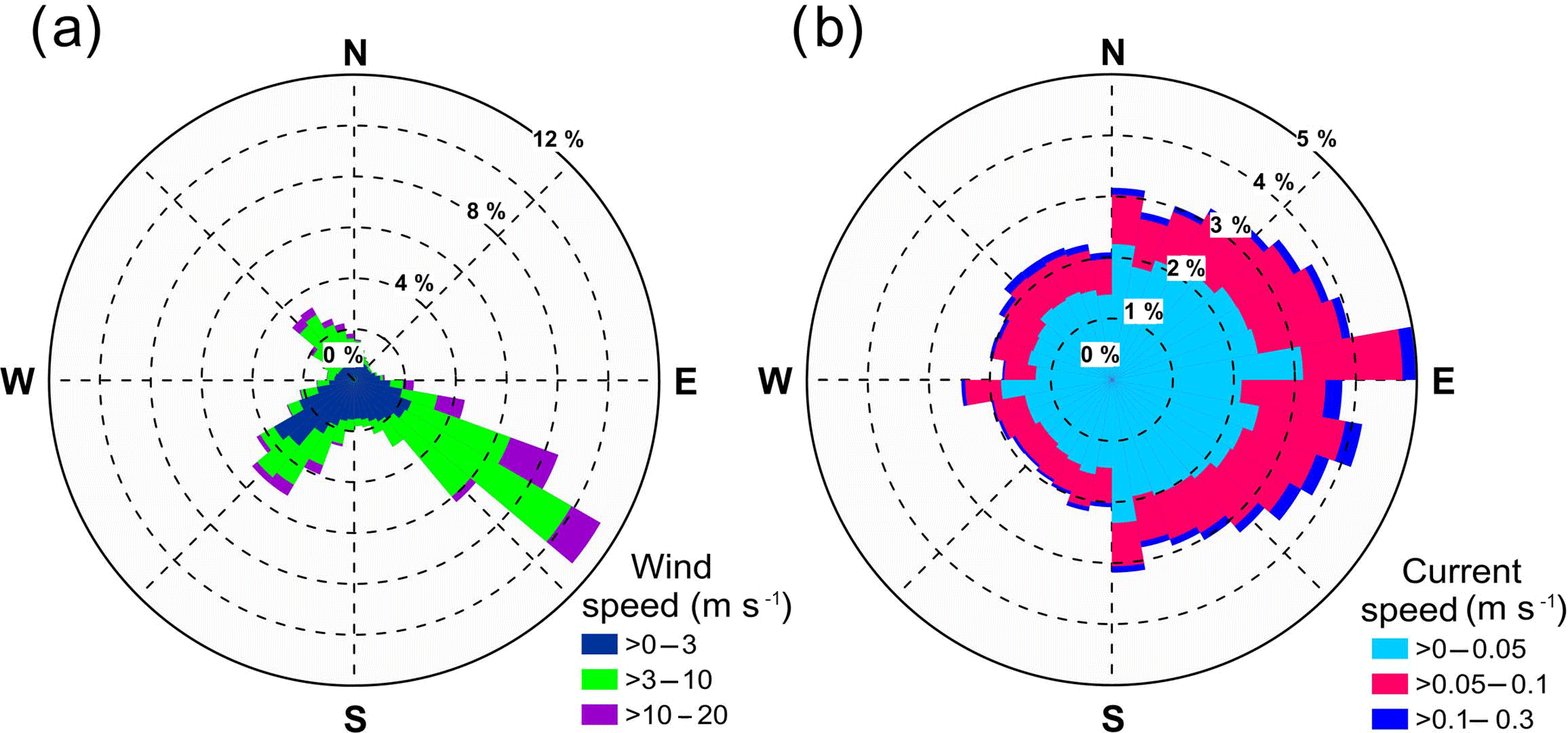
Figure 3(a) Inter-annual wind characteristics plotted via wind charts. (b) Inter-annual ocean currents. The radius expresses the frequency of the events (%), the angle represents the geographical coordinates (degrees), and the colour scale shows the wind and current intensity (m s−1).
4.2 Rain
The rain (precipitation with air temperature >0 ∘C) can help us to make inferences on the importance of surface run-off (Fig. 2a) since hydrological measurements are scarce or absent on the numerous small waterways. Daily rainfall events during the studied period were generally characterised by low intensity (on average, 3.1 mm d−1 excluding dry days). The maximum event was recorded in late December 2015 (26.5 mm) during an exceptionally warm winter week. A secondary peak occurred in September 2011 (25.4 mm). Although rainfalls were mostly low, events of long duration punctuated the analysed time series (e.g., 25 days in June 2013). Rainfalls showed a typical seasonal pattern with more frequent events during warmer seasons, especially in early September (Fig. 2a). Inter-annual variability was large during all the time intervals studied, for which summer 2013 was the wettest (cumulative values 2 to 3 times higher than 2011 and 2015 and 2012 and 2014, respectively). Finally, in contrast with the overall pattern, during winter 2015, some events of rainfall occurred in concomitance with above-zero air temperature events.
4.3 Wind
The wind speed showed a very wide variability, with the highest value reaching 26 m s−1 in February 2015 (Fig. 2b). The general mean was 4.2±2.9 m s−1. Generally speaking, during dark periods wind systematically blew at speeds of over 4 m s−1, while in summer less windy conditions prevailed. The most frequently observed wind direction was from the southeast (120∘, Fig. 3a), along the fjord axis and from the tide glacier fronts of Kongsvegen and Kronebreen (see Fig. 1). Its intensity changed very little during the years and only in 2011 and 2015 were there higher frequencies of values >15 m s−1. The second highest direction frequency was from the southwest (225∘). Its highest magnitude was observed in 2012, whereas higher frequencies of this direction occurred in 2010, 2013, and 2014. Finally, a less frequent wind direction was recorded from the northwest (320∘) from the outer fjord. It rarely showed values >15 m s−1. The wind conditions in Kongsfjorden were greatly governed by orographic steering of the large-scale wind fields and katabatic winds with cold air from the inland glaciers to the warmer fjords.
4.4 Air temperature
Air temperature modulates the surface ice melting, and hence also the englacial and subglacial water drainage network. Similar to solar radiation, air temperature also showed clear seasonal oscillations (Fig. 2b), with higher values in summer (up to 12 ∘C) and lower values in winter (down to a minimum of −24.4 ∘C). Nevertheless, there were important differences. First, minima and maxima of air temperature were delayed with respect to solar radiation by about 2 months. Second, during winter several intrusions of mild air masses occurred, except in winter 2011, the coldest season of our time series.
4.5 Oceanography
The water temperature measured at 35 m of water depth (intermediate waters) exhibited the lowest value in February 2011 (1.9 ∘C) and the highest in August 2015 (6.9 ∘C), showing a very wide range of values (Fig. 2c). Values close to the freezing point were also measured in February 2015. Relative warm peaks were usually recorded in late summer (August to September) each year, while temperature minima occurred in a longer time period (January 2011, 2012, and 2014; February 2012 and 2015; March 2013 and 2016). In the available time series, the minima of temperature showed an oscillatory pattern with values close to −1.9 ∘C in 2011, 2013, and 2015 and minimum values 1–2 ∘C higher in 2012, 2014, and 2016. Indeed, winters 2012 and 2014 showed a further peculiar character with a twin cold peak interrupted by a relatively warm time interval. Temperature maxima recorded each year did not follow the same pattern. The temperature maximum was around 3 ∘C in 2010 and exceeded 4 ∘C in 2012, but it was always higher than 6 ∘C in remaining years. Water temperatures measured at the near bottom (Fig. 2c) exhibited the highest value in October 2013 with 6.3 ∘C and lowest value in February 2011 and 2015 (−1.8 ∘C). The average values at the intermediate (2.2±2.0 ∘C) and bottom depths (2.1±1.7 ∘C) were very similar, although the near-bottom level presented slightly less dispersed values (Fig. 2c). The oscillatory pattern between the warm peaks in summer and the minima in winter was not perfectly coupled between the two levels, and often the peak value was reached earlier at the intermediate level with respect to the near-bottom one, for both highest and lowest peaks. This time lag varied up to 3 months for the warm peaks of 2011 and 2015. Superimposed on the oscillating pattern of temperatures, a general increasing trend was observed at the two levels. Based on almost 100 000 measurements for each time series, we calculated an increasing rate of 4.3 and 1.6 ∘C decade−1 at intermediate and near-bottom levels, respectively. By way of comparison, the increase in the air temperature at the Amundsen-Nobile Climate Change Tower was estimated at 3.0 ∘C decade−1 over the period 2010–2017 (Mauro Mazzola, personal communication, 2018). Salinities recorded at the near bottom showed the highest value in December 2015 (35.28) and the lowest in July 2011 (34.10). Salinities also showed periodic oscillations (Fig. 2d), although in this case the data range is narrower and the trend more confusing, with a poorly defined seasonal signal. In contrast, the long-term trend is very apparent, with an increase rate of salinity of 0.7 decade−1. The current speed at mid-depth remained quite constant during the years (Fig. 2b), with a mean value of 4.4 cm s−1. The highest values each year varied from 20 cm s−1 in February 2014 and January 2016 to 44 cm s−1 in March 2013, with intermediate values of 23–27 cm s−1 in autumn 2010, 2011, and 2012 and January 2015. Due to low current speeds, current directions were highly variable from year to year. Nevertheless, current direction was mainly toward the inner part of the fjord (Fig. 3b) with the exception of 2015, when a southward direction prevailed.
4.6 Particle fluxes
Fluxes of total particulate matter in Kongsfjorden showed a clear seasonal trend (Fig. 2e) with high values in summer and low fluxes during the rest of the year. The mean TMF was 32±57 g m−2 d−1. The highest TMF was recognised from 19 to 27 August 2013 with a peak value of 330 g m−2 d−1. Actually, all samples collected in August and early September 2013 were characterised by TMF > 200 g m−2 d−1, making summer 2013 the period with the maximum cumulative particle accumulation. After that, a secondary, more limited maximum peak in TMF was recorded in August 2015 (123 g m−2 d−1). In contrast, peak TMFs in summers 2011 and 2012 were much lower, such as those measured in 2014, although a mechanical failure during July–August 2014 prevented us from obtaining a complete time series of sediment bottles.
4.7 Particle composition
Temporal variation in the major components of the total mass flux is shown in Fig. 2f and g. The lithogenic material was the PC of the flux representing almost three-quarters of the material (range 64 %–78 %), with small seasonal and inter-annual variability. Carbonates were the second most abundant components in sediment trap samples (18.4 %–31.5 %, mean value of 23.5 %±2.6 % CaCO3). Slightly higher concentrations of carbonate were measured during periods of high TMFs (summer), especially in August–September 2013. Due to the high average values coupled with scarce seasonal variability, the major part of this component seems not to be derived by shells of living carbonatic organisms. OC and opal contents never exceed 10 % in abundances and showed a marked seasonal variability. Peak values of OC contents varied between 2.4 % in 2016 and 5.1 % in 2015 (Fig. 2g), whereas opal maxima ranged between 1.5 % in 2016 and 7.3 % in 2013. The timing of abundance peaks of the two biological components were similar, usually showing the highest values in April–June, always anticipating the TMF peaks (Fig. 2e and f). Actually, in 2013 and 2015 the OC peaks occurred 1 month later than the opal ones. During the remaining part of the year, opal contents were negligible, whereas OC varied between 0.3 % and 0.7 %. δ13C (Fig. 2h), measured in the organic fraction of C, varying from −25.9 ‰ to −21.4 ‰ (mean, −23.5 ‰), showing a clear temporal trend, which mirrored that of OC contents. For heavier δ13C values, OC contents were the highest and vice versa. The temporal pattern of IRD differed from that of other components, showing neither a clear seasonal change nor constant inter-annual fluctuations (Fig. 2g). Nevertheless, IRD variability displayed some peculiarities worthy of being described. IRD abundances displayed a peak value of 600 items m−2 d−1 in August 2013, parallel to the highest TMF. However, mean IRD abundance dropped after September 2013 from 195 items m−2 d−1 to 68 items m−2 d−1. Furthermore, the first 3 years of the time series was characterised by a more pronounced temporal variability, punctuated by at least four time intervals with higher IRD contents. Although they roughly occurred in concomitance with the peaks of TMF, their duration was longer, starting earlier than and decreasing after those of TMF. The C∕N ratio varied between 6.0 and 13.8 (mean, 9.3±1.5) in a relatively narrow range. Higher values generally mirrored those of TMF, while lower C∕N values were in agreement with the OC maximum concentrations (Fig. 2h). Exceptions to this pattern were the high values of C∕N ratios in February 2011, March 2012, January 2013, and to a lesser extent March 2014.
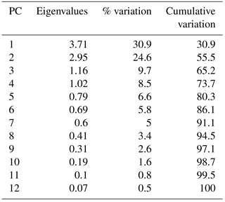
Table 2Coefficients in the linear combinations of variables making up PCs. The higher coefficients for each PC are shown in bold font.
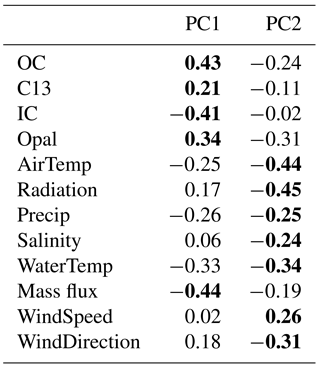
4.8 PCA
The environmental data were described through a multivariate analysis (PCA) to summarise biotic and physical data in PCs. The PCA was performed on the sediment trap samples (n=73) together with the environmental parameters averaged according to the time intervals of sediment trap samples (Table A1, Appendix). Table 1 shows 12 PCs, which account for 100 % of the variation, with PC1 and PC2 accounting for 55.5 %. The coefficients of variables for PC1 and PC2 are shown in Table 2. The major coefficients for PC1 are organic and inorganic carbon (OC, δ13C, and IC), opal, total mass flux (Mass Flux). The coefficient that displayed strong positive loadings is OM (opal, OC, and δ13C). Total mass flux, together with inorganic carbon, showed the opposite (Table 2). The main coefficient for PC2 is the wind speed, whereas air and water temperatures, radiation, precipitation, (weakly) salinity, and wind direction have opposite loadings (Table 2).
In the last decades, many studies focussing on the identification of sediment sources in the Kongsfjorden system were carried out by using different approaches (Kim et al., 2011; Kuliński et al., 2014; Lalande et al., 2016a; Svendsen et al., 2002; Trusel et al., 2010). Some studies investigated the entire fjord and others concentrated in its inner part, at the interface between fjord waters and the glacial fronts. A few studies included seasonally occupied stations in order to have a complete annual cycle (Lalande et al., 2016a; Wiedmann et al., 2016). However, multi-year time series of particle fluxes in the inner fjord have not yet been obtained; in this respect, our study is novel. The marine ecosystem of Kongsfjorden experiences pronounced seasonal variability in sunlight, glacier melt, and ice cover. As a consequence, large variations in vertical particle fluxes due to primary production (export fluxes) and lateral advection of detrital particles were expected (Lalande et al., 2016a). In the next sections, size and composition of sediment trap data will be discussed in order to elucidate which are the main atmospheric, oceanographic, biological, or sedimentological factors capable of modulating the seasonal and inter-annual variability in particle fluxes. In addition, we will focus on the full 6-year time series and, using complementary physical data, try to understand what processes trigger events of exceptionally high particle flux.
5.1 Seasonal variability in particle fluxes
Our 6-year time series of downward particle fluxes show a marked seasonal variability, confirming findings by Lalande et al. (2016a). The typical seasonal pattern of particle fluxes can be summarised as follows.
-
Spring is dominated by the export of OM with high opal and OC contents. Maximum fluxes of TMF, opal, and OC were recorded in 2013 (average TMF, 9 ± 8 g m−2 d−1, 163 ± 172 mg OC m−2 d−1, 206 ± 436 mg opal m−2 d−1).
-
Summer shows maximum values of TMF (330 g−2 d−1) consisting of lithogenic and carbonate sediments (average TMF, 85±81 g m−2 d−1, 318 ± 183 mg OC m−2 d−1, 11 ± 27 mg opal m−2 d−1).
-
Polar dark night includes low organic and inorganic fluxes (average TMF, 10 ± 6 g m−2 d−1, 66 ± 31 mg OC m−2 d−1, 3 ± 7 mg opal m−2 d−1).
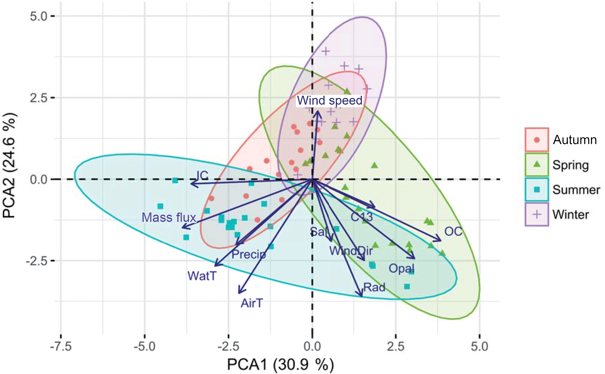
Figure 4Principal component analysis (PCA) of the collected data set arranged by seasons. The abbreviations are as follows: total mass flux (Mass Flux), organic carbon (OC), δ13C (C13), inorganic carbon (IC), opal (Opal), air temperature (AirT), wind speed and direction (WindSpeed, WindDir), solar radiation (Rad), rain precipitation (Precip), salinity (Sal), and water temperature (WatT).
In summary, TMFs in summer were about 1 order of magnitude higher than during the rest of the year. Opal fluxes in spring were from 1 to 2 orders of magnitude higher than in summer and polar night, respectively. OC fluxes showed a relatively narrower seasonal variability: maximum in summer for the contribution of mixed (fresh and ancient) OM, about one-half in spring due to export from the upper layer of newly produced phytoplankton cells, and ∼20 % of the summer fluxes during the polar night, essentially constituted by ancient OM. In order to understand to what extent the physical variables affect the environment, we have converted a set of biotic and physical observations of possibly correlated variables into a set of values of uncorrelated variables called PCs. Based on the distribution of the variables, the first axis (PC1, 30.9 % of the variance) likely describes the mixing of two different particulate sources associated with springs and summers (Fig. 4). The former was rich in freshly produced autochthonous material (high OC, opal, and δ13C values), while the latter is primarily associated with the input of glacier-derived material (high mass fluxes and high inorganic C). In addition, while the radiance explains the highly productive periods, the land-to-fjord exchange seems to be a function of the temperature in the fjord (high air and water temperature). Finally, the spring samples that show low loadings reflect periods characterised by low primary productivity associated with a pre-algal bloom period while autumn samples with negative loadings are probably related to protracted warm periods in early autumn. The second axis (PC2, 24.6 % of the variance) reflects the general seasonal trend and is dominated by the physical parameters. Along this axis, samples were grouped in two main clusters: spring–summer and autumn–winter. The former period is characterised by positive change in precipitation, temperatures, and radiance, all typical of the spring–summer periods, while autumn–winter is mainly described by the enhanced wind speed with, however, little influence on the mass flux and its composition. As Kongsfjorden is experiencing an ever-increasing warm scenario, our results from the PCA suggest that the land–ocean flux of glacier-derived material will greatly increase, while the biotic component might change to a minor extent, reflecting primarily changes in light availability (e.g., sea ice occurrence).
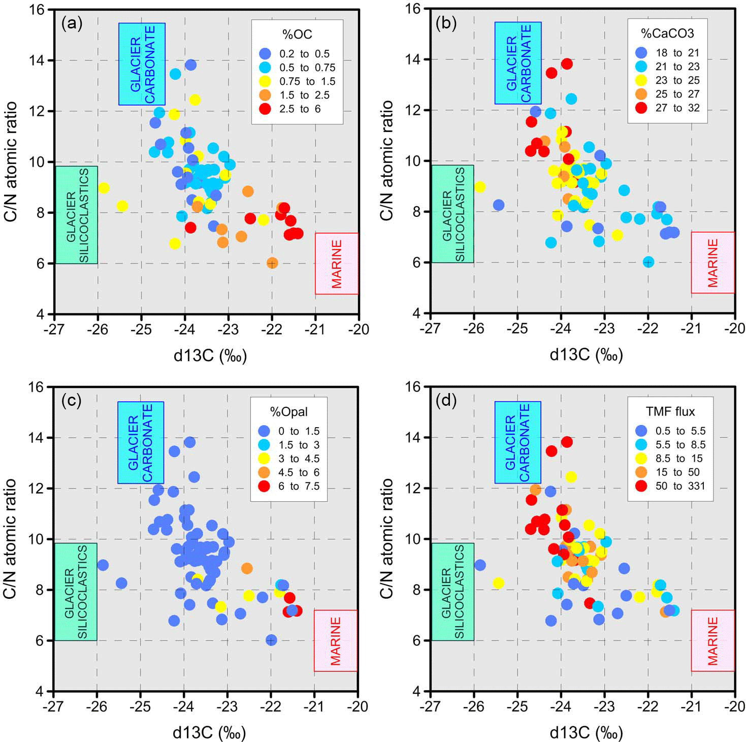
Figure 5Relationship between δ13C and C∕N for all samples plotted against % OC (a), % CaCO3 (b), opal (c), and TMF (d). Coloured areas represent the estimated ranges of organic carbon end-members.
5.2 Nature of collected particles
Particles intercepted by our sediment trap mainly consisted of silicoclastic material (Fig. 2f). Carbonates were the second most abundant component. The source of this fraction could be either biogenic, due to the contribution of organisms with carbonate shells, or clastic, as a result of erosion of old carbonate rocks by the glaciers. The PCA provides further details about the CaCO3 origin and indicates that CaCO3 dominates during the period of high mass flux associated with high summer temperatures, while the fraction of inorganic carbon is relatively low during the highly productive season. Furthermore, the CaCO3 contents were not related to the swimmer Limacina helicina abundances, the most abundant swimmer with carbonate shell in our sediment trap samples (D'Angelo et al., 2018). Altogether, this implies that most carbonate grains collected by our sediment trap are detritic, consistent with high CaCO3 concentrations observed in inner fjord sediments close to the glacier front (Bourgeois et al., 2016). Combined, silicoclastic sediment and clastic carbonates represent > 90 % of material accumulating in the inner Kongsfjorden (Fig. 2f). In the catchment area of Kronebreen and Kongsvegen glaciers, unconsolidated deposits of Quaternary age include the Gipshuken Fm with dolomite breccia, dolomites, sandstones, and marl and the Wordiekammen Fm (Dallmann, 2015). The latter contains limestones and dolomite, which are rich in calcium. Due to the geographical vicinity and compositional affinity, the Kronebreen and Kongsvegen glaciers thus seem to be the most probable sources of clastic sediment for the MDI site. To investigate the main sources that contribute to supply organic particles accumulating in the studied area, the elemental and isotopic composition of OM were considered, by plotting δ13C versus OC∕TN molar ratios (Fig. 5). In the Arctic realm, the C∕N ratio (Stein and Macdonald, 2004) and δ13C (Schubert and Calvert, 2001; Winkelmann and Knies, 2005) have been widely used as proxies to discriminate between marine and terrestrial provenance of organic material (Hedges and Oades, 1997). First results have indicated that the sediments in the Kongsfjorden–Krossfjord system primarily contain OM of marine origin (δ13C, −20.6 ‰) with respect to that of soil and coal origin (Svendsen et al., 2002; Winkelmann and Knies, 2005). Through organic chemistry analyses, and Δ14C values, Kim et al. (2011) have suggested that ancient OM of both coal-derived and mature glacial OM is buried in the Kongsfjorden–Krossfjorden system. Kuliński et al. (2014) tried to apply a three-end-member mixed model, in which the first OM source was ancient from subglacial drainage. The second one was fresh terrestrial OM from river discharges, and the third end-member was constituted by fresh marine phytoplankton. They provided the value of δ13C for the first two end-members, but found a high range of δ13C for the marine end-member, which precluded the use of the mixing model (Kuliński et al., 2014). Bourgeois et al. (2016) showed an OM composition gradient from the inner to outer Kongsfjorden reflecting a decreasing glacier contribution and a concurrent marine fraction increase. δ13C values in OM of Kongsfjorden sediments varied between −23.8 ‰ and −19.3 ‰, with the heaviest values measured in sediments collected in front of glaciers. A similar spatial variability has also been found by Kumar et al. (2016), who found that the marine OM was unusually more depleted in δ13C ( ‰) than the terrestrial OM ( ‰). Conversely, Calleja et al. (2017) indicated an input of terrigenous particulate organic carbon (POC) material coming from the turbid plumes of melting glacial ice during August and October characterized by δ13C values consistently depleted in δ13C (ranging from −25.6 to −27.1 ‰) and the highest value of −22.7 ‰ occurring in May at the peak of Chl a concentration, consistent with phytoplankton end-members commonly used. These apparent discrepancies could be reconciled in view of the higher temporal variability in stable isotope composition with respect to the spatial one. The distribution pattern of C∕N and δ13C values of our samples (Fig. 5) shows a quasi-triangular shape, suggesting three main sources of OM collected by the sediment trap of mooring MDI. Consistent with our early discussion based on the PCA results, the first end-member is marine particulate material characterised by low C∕N ratios, relatively heavier δ13C values, and high opal and OC contents (Fig. 5). The second end-member is instead associated with the material released by the glacier and it was characterised by high TMF and C∕N ratios, relatively low δ13C values, lack of opal, and being rich in CaCO3 (Fig. 5). The third end-member remains elusive, though. Low opal contents do not support the hypothesis of in situ diatom production while the relatively high OC content would suggest glacier outflows quantitatively enriched in fossil–subfossil bioavailable carbon since glaciers may be eroding ancient peatlands (Hood et al., 2009); in fact, during the warmer parts of the Holocene many of Svalbard's glaciers retreated onto land and proglacial areas were covered by tundra (Lydersen et al., 2014). Overall, the depleted δ13C values might suggest a land-derived origin. However, the isotopic fingerprint of the largest river (Bayelva, Fig. 1) discharging into the fjord displays relatively heavier compositions (range ‰) (Zhu et al., 2016). In addition, although the coal-derived OM is another potential source due to the mining activity that occurred over the last century, its input is mainly constrained to the region adjacent to Ny-Ålesund coast (Kim et al., 2011) and, anyhow, it would result in remarkably high C∕N ratios. Finally, the contemporary input of soil OM into the fjord can be considered negligible, likely due to the limited soil formation in the cold Arctic environment, which weakens the signature of soil OM in marine environments (Kim et al., 2011). Altogether, our results might suggest the input of a second OM pool from the glacier in addition to the carbonate-rich end-member. This input, generally referred to as silicoclastic-rich material, might be associated with a different glacier or rock source. However, additional analyses (e.g., biomarkers) are needed to further refine the third OC source to the inner fjord.
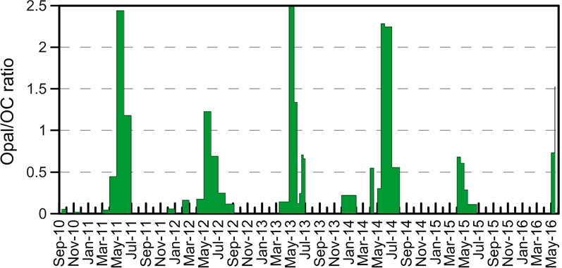
Figure 6Ratio between the opal and OC contents within sediment trap samples from September 2010 to May 2016.
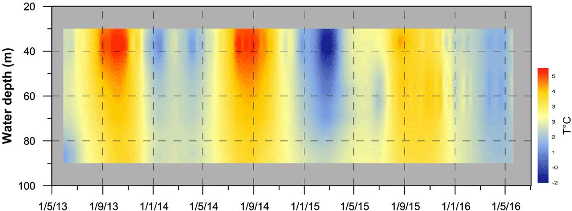
Figure 7Temporal variability in the water temperature section, reconstructed between May 2013 and June 2016 based on measurements at four levels (36–37 m, 54–58 m, 62–69 m, 87 m).
5.3 Factors governing particle fluxes of marine origin
Elevated vertical fluxes of fresh OM of marine origin, as well as high OC and opal contents (Fig. 2f and g), in spring indicate the occurrence of substantial algal blooms (Lalande et al., 2016a). Typically, Kongsfjorden spring blooms peak in May and consist of diatoms and Phaeocystis pouchetii (Hegseth and Tverberg, 2013). The higher proportion of opal with respect to OC (Fig. 6) in spring samples corroborates the interpretation of periods characterized by high diatom export fluxes, whereas in time intervals with lower opal∕OC ratios, a mixed phytoplankton composition probably prevails. The phytoplankton growth is mainly driven by the availability of light and nutrients, although other factors can influence algal dynamics (e.g., water temperature, zooplankton grazing, water stratification). In the Arctic region, it has been established that seasonality is mainly driven by the light regime and the angle of the sun, rather than temperature (Berge et al., 2015). The seasonal pattern of fresh marine OM of our time series clearly shows that export fluxes in April–June (Fig. 2g) were closely coupled with the algal blooms, which occur when light is enough to trigger primary productivity (Fig. 2a), suggesting that in Kongsfjorden solar radiation exerts a first-order control on the timing of phytoplankton blooms and on the following export fluxes. The nutrient availability is instead less predictable than the seasonal irradiance and in the ocean it can be a function of the water mixing, which results in the intrusion of nutrient-rich waters into the euphotic zone. To test if convective mixing takes place during winter in Kongsfjorden, we analysed a time series section of water temperature (Fig. 7) extrapolated by measurements recorded at four levels (36–37 m, 54–58 m, 62–69 m, 87 m) between May 2013 and June 2016. Vertical temperatures showed large temporal differences. Overall, warmer periods occur in late summer and autumn. In contrast, colder water periods characterise winter and early spring. In both cases, the portion of water column investigated (30–90 m) appears stratified. The shift between the two conditions is rapid with a complete mixing of the water column. The greater intrusion of AW at mid-depth is probably responsible for the heating of the interior of the water column, while the cooling of surface waters during winters with the formation of local dense waters by low air temperatures and the high wind regime triggers the convective mixing and sinking of the newly formed waters to the bottom. However, year-to-year differences were recorded with winter AW intrusions in January–February 2012, 2014, and 2016 (Figs. 2c and 9), which prevented a complete mixing of the water column and, presumably, a less efficient upward nutrient supply. When this occurs, the relatively less abundance of nutrients results in low primary productivity in the inner fjord. If our interpretation is correct, then the inter-annual variability in spring export fluxes in Kongsfjorden is driven by nutrient supply and, ultimately, by the different year-to-year winter intrusion of AW. The anomalous inflow events of warm AW in winter can also prevent sea ice formation in Kongsfjorden, delaying the bloom timing by 3–4 weeks in spring (Hegseth and Tverberg, 2013). Specifically, three scenarios have been described (Hegseth and Tverberg, 2013).
-
Sea ice in the fjord during winter, and lots of ice outside, with a normal inflow of AW along the bottom, leads to a May bloom.
-
Open water in the fjord in combination with ice outside the fjord, with a normal inflow of AW along the bottom, leads to an April bloom.
-
Both the fjord and adjacent shelf being open, and an unusual surface inflow of AW to the fjord in winter, leads again to a May bloom.
During the investigated period, Kongsfjorden was covered by sea ice only in winter 2011; thus we expected that the algal bloom occurred in May. In the following years, the sea ice coverage was negligible (Payne, 2015). In 2012, 2016, and especially in 2014, due to the incursion of AW between January and March, the algal blooms were probably delayed following scenario (3). This is confirmed by the modest OM export in our sediment trap (Fig. 2g). Finally, the algal blooms in 2013 and 2015 followed scenario (2), with export fluxes occurring earlier, in late April. In summary, the seasonal signal of export fluxes is triggered by solar light. The onset of OC export can change from year to year from late April to late May (Fig. 2g) depending on absence or presence of sea ice cover and on the AW intrusion during the previous winter. The winter incursion of AW into the fjord also affects the input of nutrients from bottom waters modulating the magnitude of the primary production and the corresponding inter-annual variability in export fluxes.
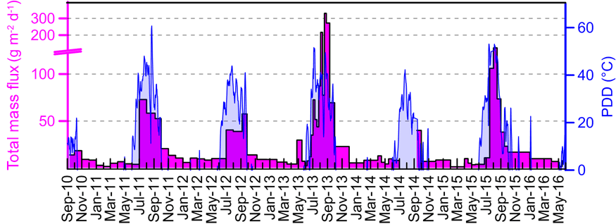
Figure 8Total mass fluxes plotted against the 6-day PDD sum, as a proxy of subglacial run-off.
5.4 Lateral advection of clastic particles: temporal variability, sources, and mechanisms of delivery
The majority of downward particle fluxes are restricted to a short period in the summer: in July–September, the mass flux accounts for 38 % to 71 % of the annual flux, depending on the collection year. As previously described, particles in summer are almost completely constituted by terrigenous sediments (on average, ∼99 %), both carbonate and silicoclastic. In line with what is shown by the PCA (Fig. 4), the total mass fluxes peak in July–August, after the solar radiation maxima (late June) (Fig. 2a), but perfectly in phase with air temperature (Fig. 2b) and partially with rain (Fig. 2a). The highest water temperature values are instead slightly delayed, occurring in August to September (Fig. 2g). In the previous paragraphs, we inferred that glaciers are the most probable source of clastic sediment for site MDI. Air temperature strongly affects glacier drainage, which in summer begins once there is sufficient surface melt to warm the glacier snowpack to the melting point, allowing water to make its way downward to the subglacial drainage network (Lydersen et al., 2014). As surface water enters this subglacial network, overpressure occurs, leading to lift-up and entrainment of basal sediments. As a result, the water coming out of the glacier tends to be sediment laden (Hodgkins et al., 1999). Conversely, when air temperature decreases below zero, during winter months, the processes of meltwater refreezing and water storage switch to a slow drainage system (Lydersen et al., 2014). This produces a pronounced seasonality in freshwater (Jansson et al., 2003) and sediment discharge, and ultimately in downward particle fluxes in the inner fjord, as recorded by our sediment trap (Fig. 2f). In order to test if meltwater run-off is the most important factor driving the suspended matter supply to the fjord, we used positive degree days (PDDs) as a proxy for meltwater availability. Following the methods of Schild and Hamilton (2013), the daily average temperature after the onset of melt is defined as the PDD value for each day. To take into account lags in the hydraulic system introduced by finite transit time of meltwater through the glacier system and potential subglacial storage, we calculated a “lag index” using accumulated PDDs. This index is the cumulative sum of the PDDs in the 6 days prior to that day (Schild et al., 2017). The perfect synchronicity of TMF and accumulated PDD (Fig. 8) suggests that glacial meltwater run-off, the subglacial transport of meltwater, is the main process able to supply clastic sediment to Kongsfjorden, and that the seasonal variability in air temperature, specifically the accumulated temperature above the melting point, ultimately modulates the timing of TMF at site MDI as well.
It has been recently shown (Luckman et al., 2015) that ocean temperature strongly impacts the calving rates of tidewater glaciers. In Kongsfjorden, submarine melting is specifically forced by the AW intrusions. However, the delay of maximum water temperature (Fig. 2c) from the TMF peaks (Fig. 2f) would suggest that submarine melting is a minor font of sediment for site MDI and can at best explain the slow declining trend in TMF during some autumns (e.g., in 2011, 2013 and 2015; Fig. 2f).
Marine currents measured at mid-depth of mooring MDI were mostly directed toward the inner fjord (Fig. 3b), whereas winds coming from the glacier valleys (Fig. 3a) force the surface water to move out of the fjord (Aliani et al., 2016). It results that water circulation in the innermost part of Kongsfjorden is of an estuarine-like type with cold freshwater on top of warm saline water (Aliani et al., 2016; Cottier et al., 2005; Sundfjord et al., 2017; Svendsen et al., 2002; Trusel et al., 2010). This type of circulation implies that the glacially derived sediment will spread at the surface through hypopycnal sediment-rich plumes dispersed by winds over the fjord. Specifically, the primary driver of hypopycnal plume formation is a meltwater upwelling from Kronebreen (Trusel et al., 2010). As meltwater discharges from the base of the glacier, it entrains high concentrations of sediment and rapidly forms a turbulent jet (Powell, 1991). Because of relative density contrasts, the jet rises vertically and forms a buoyant and brackish surface overflow plume. At the surface, the brackish plume spreads laterally (Trusel et al., 2010) driven by the wind.
Finally, PCA results (Fig. 4) suggest that even the surface run-off by rainfalls can increase the sediment delivery to the fjord, especially in summer 2013 (Fig. 2a), making the upper water very turbid and resulting in typical red waters. Winter precipitation events in Ny-Ålesund have increased during recent years (on average 3 %–4 % decade−1 for the 1961–2010 period (Førland et al., 2011). As a matter of fact, the concurrent air temperature increase may enhance the rain fraction against snow. The rain events recorded in January–February 2016 (Fig. 2a) testify the incursion of mild and wetter air masses into the fjord. Therefore, in a warming scenario, an increase in particle flux to Kongsfjorden by local watersheds can be expected, even during winter.
5.5 Annual fluxes and possible changes
TMFs measured at the MDI station are about 20–100 times higher compared to downward fluxes measured on the Spitsbergen continental margin (Lalande et al., 2016b; Sanchez-Vidal et al., 2015) but are of the same order of those measured in August 2012 in Kongsfjorden by Lalande et al. (2016a). For studying the variability in particle fluxes at a multi-year scale, the use of annual time-averaged TMFs is preferable. The lowest time-weighted averages were calculated for 2010, 2014, and 2016 (4.6×10³, 3.8×10³, 3.1×10³ g m−2 year−1, respectively), but these time-weighted TMFs could be underestimated because the time series were not complete and missed the summer, the most abundant flux season. The inter-annual time-weighted TMFs varied by a factor of 2 over time (6.8×10³ to 14.7×10³ g m−2 for 2012 and 2013, respectively).
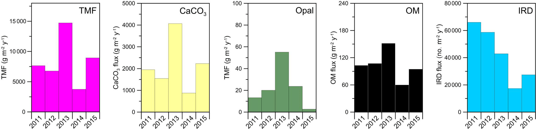
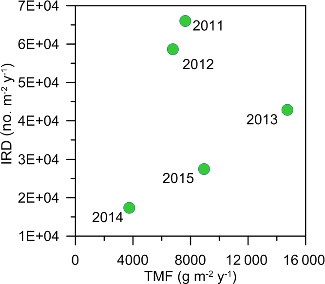
Annual total mass and main component fluxes do not show any clear temporal trend (Fig. 9). In 2013, the highest fluxes resulted from the combined effect of enhanced subglacial run-off (as pointed out by air temperature and PDD), submarine melting (water temperature), and surface run-off (rain). In contrast, IRD fluxes strongly decrease over time (Fig. 9). IRD abundance in sediment cores is commonly used in palaeoceanographic reconstructions as a proxy for iceberg production and transit. However, the water temperature affecting the calving rate, and hence the iceberg production, showed an increasing temporal trend in Kongsfjorden during 2010–2016, which would imply an enhanced submarine melting. Conversely, annual TMF and IRD fluxes in 2013–2015 seem well correlated, supporting a common source from glacier melting (Fig. 10), while an additional source of IRD must be taken into account for the years 2011 and 2012. At least for 2011, when the fjord froze for the last time, we tentatively suggest that the source of this extra IRD may be linked to the summer melting of “dirty” sea ice formed in the previous winter by suspension freezing or entrainment via anchor ice (Darby et al., 2011). Alternatively, we can argue that the sediment deposits at Kronebreen and Kongsvegen glacier termini reduced the relative depth of water over time, resulting in increased glacier stability through decreased rates of iceberg calving (Kehrl et al., 2011), and hence also lower IRD fluxes along the iceberg transit pathway.
As previously discussed, the variability in biogenic fluxes (OM and opal) mainly depends on the nutrient supply and indirectly on the efficiency of convective mixing during winter as a balance between the winter AW intrusion and local dense-water formation. Our 6-year time series is still too short for obtaining reliable long-term prediction, but the increasing trends in salinity (0.7 decade−1) and temperature (1.6 to 4.3 ∘C decade−1 at near bottom and mid-depth, respectively), such as the year-to-year alternation of deep and shallow convective mixing are objectively clear. The warming of the AW entering Kongsfjorden would most likely continue to hinder the formation of ice cover, contributing to phytoplankton assemblage changes but also to more frequent conditions of shallower water mixing and lower nutrient supply, with a consequent expected reduction of magnitude of primary production and export fluxes. This scenario has already occurred in Adventfjorden during 2007–2008 (Zajączkowski et al., 2010). Although the increase in the air temperature at CCT is a straight signal over the period 2010–2017 (Fig. 2a), the accumulated PDD, as well as TMFs, varied more randomly. Nevertheless, on a decadal timescale, the consistent rise of air and ocean temperature will result in further higher glacier meltwater with the increase in both TMF and clastic contribution.
Our 6-year time series of marine particle fluxes and physical parameters in Kongsfjorden provided an extraordinary opportunity to investigate seasonal and multi-year changes in the inner fjord. Our results suggest that, as the Arctic temperature rises in a warming scenario, the flux of glacier-derived material will increase accordingly. In particular, our time series points towards the subglacial run-off driven by air temperature being the dominant process affecting the glacier–fjord discharge of lithogenic material. Furthermore, the watershed run-off is also expected to increase the sediment delivery from land. The quantity of photosynthetically available radiation will likely increase due to reduced sea ice coverage. Conversely, the increased turbidity will decrease the light penetration into subsurface water, diminishing the primary production. Furthermore, water column stratification modulated by the inflow of warm Atlantic waters, especially in winter, will progressively hamper the exchange of nutrients from the bottom waters. This, in turn, will severely reduce the biological production and in particular the primary productivity in the fjord. Altogether, we infer that Kongsfjorden will experience a progressive increase in the glacier-derived fluxes and watershed run-off (i.e. lateral component) at the expense of in situ production (i.e. vertical component).
Total mass fluxes and content of major constituents of sediment trap samples are available in Table A1. The meteorological and hydrological time series are available upon request to Leonardo Langone (leonardo.langone@ismar.cnr.it).
Samples are stored at the CNR ISMAR facilities in Bologna, Italy, and are available upon request to Leonardo Langone (leonardo.langone@ismar.cnr.it).
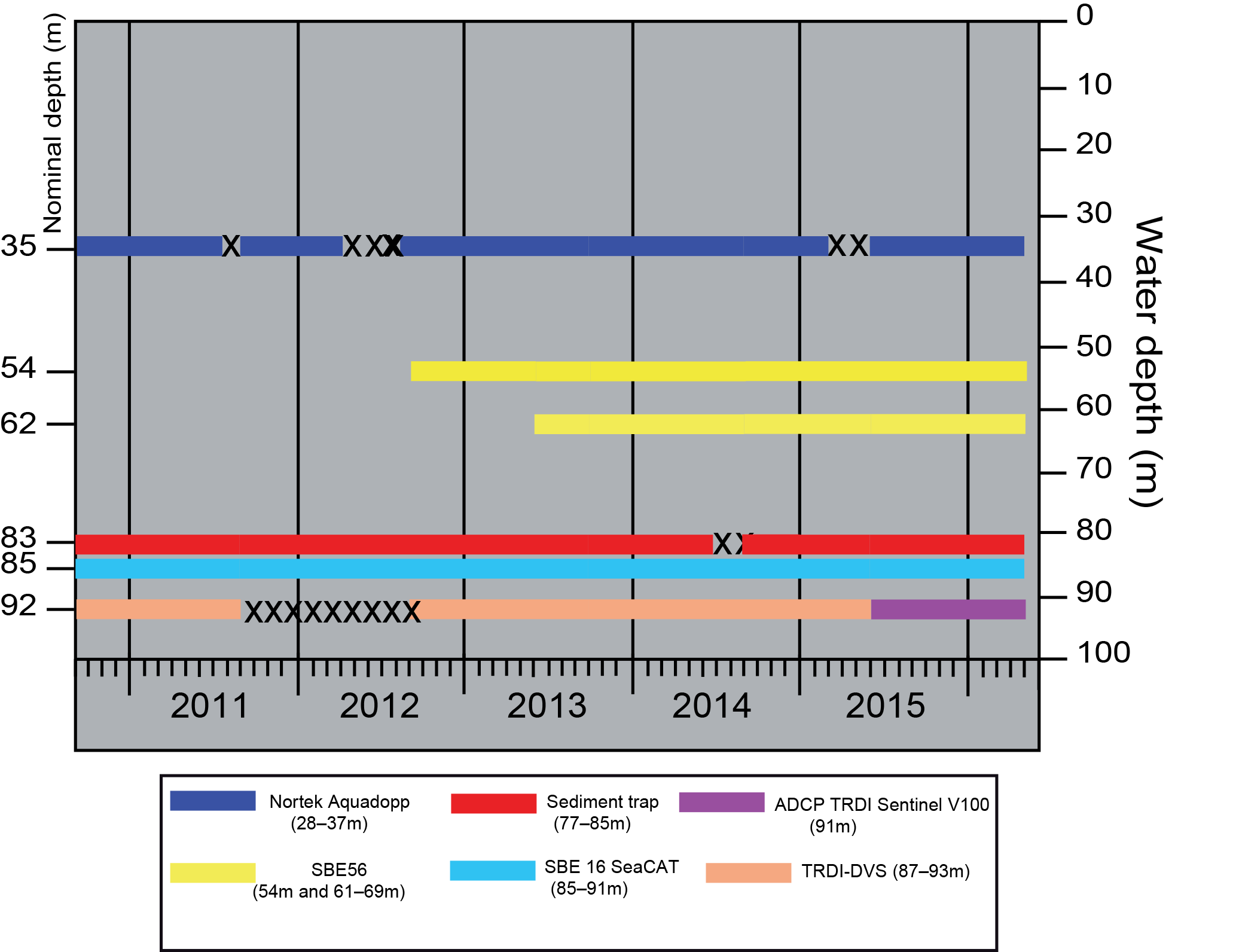
Figure A1List of available time series for each instrument mounted on MDI in the period 2010–2016. No instrument was set at the surface because of the risk of damage from iceberg transit and sea ice coverage. The “X” symbol indicates an instrument malfunctioning.
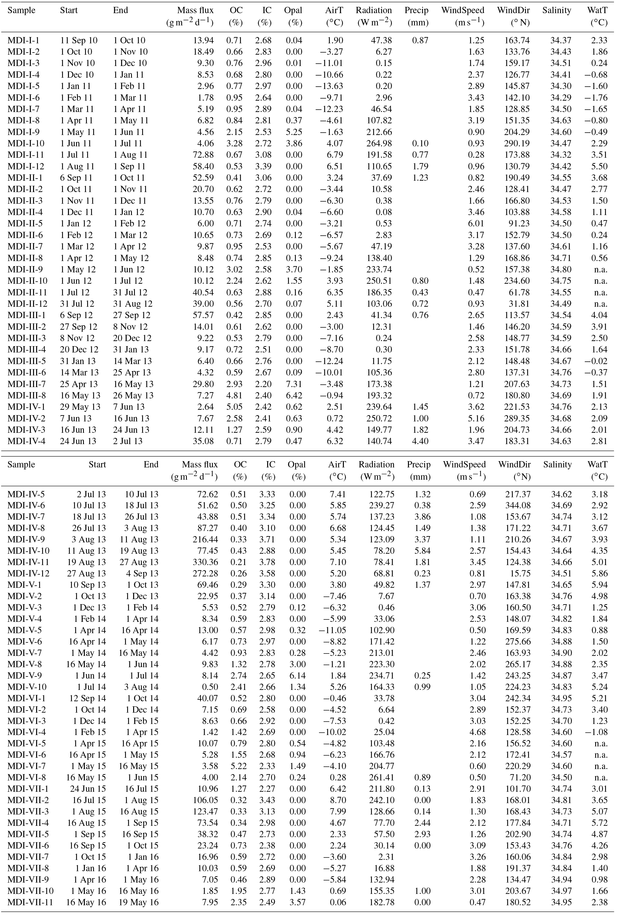
Table A1Sediment trap data set, with meteorological and hydrological data. Physical data were averaged according to the sampling periods.
LL, SM, FG, and SA designed the experiments and, together with AD'A, performed the sampling procedure and the measurements. AV and MM were involved in the implementation of the research by processing the meteorological data. AD'A carried out the preliminary treatment on sediment trap samples and together with AS-V carried out the opal analysis. LL, SM, and AD'A processed the hydrological data set. TT, LL, and AD'A were involved in the interpretation of the results. AD'A wrote the paper with input from all co-authors and produced the figures.
The authors declare that they have no conflict of interest.
We would like to thank the staff of Arctic station Dirigibile Italia and
Kings Bay AS for logistic support. We acknowledge the captains and
crew of the MS Teisten for their help during mooring deployment
and recovery. We also thank Giuliana Panieri (Tromsø) and Philippe Kerherve'
(Perpignan) for fruitful discussions on an early version of the paper and the two
anonymous referees, who greatly improved the final version. Kyle Mayers
(NOCS) is thanked
for helping in statistics. This project was funded by Progetto Premiale MIUR
ARCA, coordinated by the Department of Earth Sciences and Technologies for
the Environment of the Italian National Research Council. This is
contribution number 1968 of CNR-ISMAR of Bologna.
Edited by: Jean-Pierre Gattuso
Reviewed by:
two anonymous referees
ACIA: Impacts of a Warming Arctic: Arctic Climate Impact Assessment, Cambridge University Press, Cambridge, ISBN: 0521617782, 2004. a
Aliani, S., Sciascia, R., Conese, I., D'Angelo, A., Del Bianco, F., Giglio, F., Langone, L., and Miserocchi, S.: Characterization of seawater properties and ocean heat content in Kongsfjorden, Svalbard Archipelago, Rendiconti Accademia dei Lincei, 27, 155–162, https://doi.org/10.1007/s12210-016-0544-4, 2016. a, b, c
Aliani, S., Viola, A., Mazzola, M., D'Angelo, A., Giglio, F., Miserocchi, S., Tesi, T., and Langone L.: Coupled marine and atmospheric observations in Kongsfjorden (Svalbard) in 2010–2018, in preparation, 2018. a
Berge, J., Daase, M., Renaud, P. E., Ambrose, W. G., Darnis, G., Last, K. S., Leu, E., Cohen, J., Johnsen, G., Moline, M., Cottier, F., Varpe, Ø., Shunatova, N., Bałazy, P., Morata, N., Massabuau, J., Falk-Petersen, S., Kosobokova, K., Hoppe, C., Węsławski, J., Kukliński, P., Legeżyńska, J., Nikishina, D., Cusa, M., Kędra, M., Włodarska-Kowalczuk, M., Vogedes, D. Camus, L., Tran, D., Michaud, E., Gabrielsen, T., Granovitch, A., Gonchar, A., Krapp, R., and Callesen, T.: Unexpected levels of biological activity during the polar night offer new perspectives on a warming Arctic, Curr. Biol, 25, 2555–2561, https://doi.org/10.1016/j.cub.2015.08.024, 2015. a
Beszczynska-Möller, A., Fahrbach, E., Schauer, U., and Hansen, E.: Variability in Atlantic water temperature and transport at the entrance to the Arctic Ocean, 1997–2010, J, Marine Sci,, 69, 852–863, https://doi.org/10.1093/icesjms/fss056, 2012. a, b, c
Blaszczyk, M., Jania, J., and Hagen, J.: Tidewater glaciers of Svalbard: recent changes and estimates of calving fluxes, Pol. Polar Res., 30, 85–182, 2009. a, b
Bourgeois, S., Kerhervé, P., Calleja, M., Many, G., and Morata, N.: Glacier inputs influence organic matter composition and prokaryotic distribution in a high Arctic fjord (Kongsfjorden, Svalbard), J. Marine Syst., 164, 112–127, 2016. a
Calleja, M., Kerhervé, P., Bourgeois, S., Kedra, X., Leynaert, A., Devred, E., Babin, M., and Morata, N.: Effect of increase glacier discharge on phytoplankton bloom dynamics and pelagic geochemistry in a high Arctic fjord, Prog, Oceanography, 159, 195–210, 2017. a
Carmack, E. C., Yamamoto-Kawai, M., Haine, T. W. N., Bacon, S., Bluhm, B. A., Lique, C., Melling, H., Polyakov, I. V., Straneo, F., Timmermans, M.-L., and Williams, W. J. F. A.: Freshwater and its role in the Arctic Marine System: Sources, disposition, storage, export, and physical and biogeochemical consequences in the Arctic and global oceans., J. Geophys. Res.- Biogeo.,, 121, 675–717, https://doi.org/10.1002/2015JG003140, 2016. a
Chiarini, F., Capotondi, L., Dunbar, R., Giglio, F., Mammì, I., Mucciarone, D., Ravaioli, M., Tesi, T., and Langone, L.: A revised sediment trap splitting procedure for samples collected in the Antarctic sea, Methods Oceanogr., 8, 13–22, https://doi.org/10.1016/j.mio.2014.05.003, 2014. a, b
Cottier, F., Tverberg, V., Inall, M., Svendsen, H., Nilsen, F., and Griffiths, C.: Water mass modification in an Arctic fjord through cross-shelf exchange: The seasonal hydrography of Kongsfjorden, Svalbard, J. Geophys. Res., 110, C12005, https://doi.org/10.1029/2004JC002757, 2005. a, b, c
Dallmann, W. K.: Geoscience Atlas of Svalbard, Norwegian Polar Institute, Report 148, Tromsoe, 2015. a
D'Angelo, A., Mayers, K., Renz, J., Conese, I., Miserocchi, S., Giglio, F., and Langone, L.: A 7-year time series of mesozooplankton abundance in Kongsfjorden, Svalbard, in preparation, 2018. a
Darby, D. A., Myers, W. B., Jakobsson, M., and Rigor, I.: Modern dirty sea ice characteristics and sources: The role of anchor ice, J. Geophys. Res, 116, C09008, https://doi.org/10.1029/2010JC006675, 2011. a
Dowdeswell, J. and Forsberg, C.: The size and frequency of icebergs and bergy bits derived from tidewater glaciers in Kongsfjorden, northwest Spitsbergen, Polar Res., 2, 81–91, 1992. a, b
Fabres, J., Calafat, A., Sanchez-Vidal, A., Canals, M., and Heussner, S.: Composition and spatio-temporal variability of particle fluxes in the Western Alboran Gyre, Mediterranean Sea, J. Marine Syst., 33–34, 431–456, 2002. a
Førland, E. J., Benestad, R., Hanssen-Bauer, I., Haugen, J. E., and Skaugen, T. E.: Temperature and Precipitation Development at Svalbard 1900–2100, Adv. Meteorol., 2011, 893790, https://doi.org/10.1155/2011/893790, 2011. a
Hagen, J. O., Liestøl, O., Roland, E., and Jørgensen T.: Glacier atlas of Svalbard and Jan Mayen, Nor. Polarinst. Medd. 129, Norwegian Polar Institute, Oslo, 1993. a
Harms, A. P., Tverberg, V., and Svendsen, H.: Physical qualification and quantification of the water masses in the Kongsfjorden-Krossfjorden system cross section, OCEANS 2007 – Europe, Aberdeen, UK, 18–21 June 2007, 1–6, https://doi.org/10.1109/OCEANSE.2007.4302332, 2007. a
Hedges, J. I. and Oades, J. M.: Comparative organic geochemistries of soils and marine sediments, Org. Geochem., 27, 319–361, 1997. a
Hegseth, E. N. and Tverberg, V.: Effect of Atlantic water inflow on timing of the phytoplankton spring bloom in a high Arctic fjord (Kongsfjorden, Svalbard), J. Marine Syst., 113–114, 94–105, 2013. a, b
Hodgkins, R., Hagen, J. O., and Hamran, S. E.: 20th-century mass balance and thermal regime change at Scott Turnerbreen, Svalbard, Ann. Glaciol., 28, 216–220, 1999. a
Hood, E., Fellman, J., Spencer, R. G. M., Hernes, P. J., Edwards, R., D'Amore, D., and Scott, D.: Glaciers as a source of ancient and labile organic matter to the marine environment, Nature, 462, 1044–1048, 2009. a
Howe, J., Moreton, S., Morri, C., and Morris, P.: Multibeam bathymetry and the depositional environments of Kongsfjorden and Krossfjorden, western Spitsbergen, Svalbard, Polar Res., 22, 301–316, 2003. a, b
IPCC: Climate Change 2014: Synthesis Report. Contribution of Working Groups I, II and III to the Fifth Assessment Report of the Intergovernmental Panel on Climate Change, edited by: Core Writing Team, Pachauri, R. K., and Meyer, L. A., IPCC, Geneva, Switzerland, 151 pp., 2014. a
Jansson, P., Hock, R., and Schneider, T.: The concept of glacier storage: a review, J. Hydrol., 282, 116–129, 2003. a
Kamatani, A. and Oku, O.: Measuring biogenic silica in marine sediments, Mar. Chem., 68, 219–229, 2000. a
Karl, D. M. and Knauer, G. A.: Swimmers a recapitulation of the problem and a potential solution, Oceanography, 2, 32–35, https://doi.org/10.5670/oceanog.1989.28, 1989. a
Kehrl, L. M., Hawley, R., Powell, R. D., and Brigham-Grette, J.: Glacimarine sedimentation processes at Kronebreen and Kongsvegen, Svalbard, J. Glaciol., 57, 841–847, 2011. a
Kim, J.-H., Peterse, F., Willmott, V., Kristensen, D. K., Baas, M., Schouten, S., and Sinninghe Damsté, J.: Large ancient organic matter contributions to Arctic marine sediments (Svalbard), Limnol. Oceanogr., 56, 1463–1474, https://doi.org/10.4319/lo.2011.56.4.1463, 2011. a, b, c, d
Kristensen, E. and Andersen, F.: Determination of organic carbon in marine sediments: a comparison of two CHN-analyzer methods, J. Exp. Mar. Biol. Ecol., 109, 15–23, 1987. a
Kuliński, K., Kedra, M., Legezyska, J., Gluchowska, M., and Zaborska, A.: Particulate organic matter sinks and sources in high Arctic fjord, J. Marine Syst., 139, 27–37, https://doi.org/10.1016/j.jmarsys.2014.04.018, 2014. a, b, c
Kumar, V., Tiwari, M., Nagoji, S., and Tripathi, S.: Evidence of anomalously low delta 13C of Marine Organic Matter in an Arctic Fjord, Sci. Rep., 6, 36192, https://doi.org/10.1038/srep36192, 2016. a
Lalande, C., Moriceau, B., Leynaert, A., and Morata, N.: Spatial and temporal variability in export fluxes of biogenic matter in Kongsfjorden, Polar Biol., 39, 1725–1738, 2016a. a, b, c, d, e, f
Lalande, C., Nöthig, E.-M., Bauerfeind, E., Hardge, K., Beszczynska-Möller, A., and Fahl, K.: Lateral supply and downward export of particulate matter from upper waters to the seafloor in the deep eastern Fram Strait, Deep-Sea Res., 114, 78–89, 2016b. a
Liestøl, O.: The glaciers in the Kongsfjorden area, Spitsbergen, Norsk geogr Tidsskr, 42, 231–238, 1988. a, b
Luckman, A., Benn, D. I., Cottier, F., Bevan, S., Nilsen, F., and Inall, M.: Calving rates at tidewater glaciers vary strongly with ocean temperature,, Nat. Commun., 6, 8566, https://doi.org/10.1038/ncomms9566, 2015. a
Lydersen, C., Assmy, P., Falk-Petersen, S., Kohler, J. J., Kovacs, K., Reigstad, M., Steen, H., Strøm, H., Sundfjord, A., Varpe, Ø., Walczowski, W., Weslawski, J., and Zajaczkowski, M.: The importance of tidewater glaciers for marine mammals and seabirds in Svalbard, Norway, J. Marine Syst., 129, 452e471, https://doi.org/10.1016/j.jmarsys.2013.09.006, 2014. a, b, c
MacLachlan, S., Howe, J., and Vardy, M.: Morphodynamic evolution of Kongsfjorden-Krossfjorde, Svalbard, during the Late Weichselian and the Holocene, in: Fjord Systems and Archives, edited by: Howe, J., Austin, W., Forwick, M., and Paetzel , M., Special Publications of Geological Society, London, 344, 195–205, 2010. a, b
Majewski, W., Szczuciński, W., and Zajączkowski, M.: Interactions of Arctic and Atlantic water-masses and associated environmental changes during the last millennium, Hornsund (SW Svalbard), Boreas, 38, 529–544, https://doi.org/10.1111/j.1502-3885.2009.00091.x, 2009. a
Mazzola, M., Viola, A. P., Lanconelli, C., and Vitale, V.: Atmospheric observations at the Amundsen-Nobile Climate Change Tower in Ny-2004, Svalbard, Rend. Fis. Acc. Lincei, 27, 1–7, https://doi.org/10.1007/s12210-016-0540-8, 2016. a
Meslard, F., Bourrin, F., Many, G., and Kerherve, P.: Suspended particle dynamics and fluxes in an Arctic fjord (Kongsfjorden, Svalbard), Estuar. Coast Shelf S., 204, 212–224, https://doi.org/10.1016/j.ecss.2018.02.020, 2018. a
Mortlock, R. A. and Froelich, P. N.: A simple method for the rapid determinations of biogenic opal in pelagic marine sediments, Deep-Sea Res., 36, 1415–1426, 1989. a
Overpeck, J., Hughen, K., Hardy, D., Bradley, R., Case, R., Douglas, M., Finney, B., Gajewski, K., Jacoby, G., Jennings, A., Lamoureux, S., Lasca, A., MacDonald, G., Moore, J., Retelle, M., Smith, S., Wolfe, A., and Zielinski, G.: Arctic Environmental Change of the Last Four Centuries, Science, 278, 1251–1256, https://doi.org/10.1126/science.278.5341.1251, 1997. a
Payne, C. M.: Characterizing the influence of Atlantic water intrusion on water mass formation and primary production in Kongsfiorden, Svalbard, Tech. rep., Student Scholarship and Creative Work at Bowdoin Digital Commons, Honors Projects, Paper 23, 2015. a
Powell, R. D.: Grounding-line systems as second-order controls on fluctuations of tidewater termini of temperate glaciers, in: Glac. Mar. Sedim. Paleoclimatic Significance, Geological Society of America Special Paper 94, 75–94, 1991. a
Rajagopalan, D. M.: Characterizing fjord oceanography Near Tidewater Glaciers Kronebreen and Kongsvegen, in Kongsfjorden, Svalbard (REU Oceanographic Data Report), Yale College, 2012. a
Ragueneau, O., Savoye, N., Del Amo, Y., Cotten, J., Tardiveau, B., and Leynaert, A.: A new method for the measurement of biogenic silica in suspended matter of coastal waters: Using Si:Al ratios to correct for the mineral interference, Cont. Shelf Res., 25, 697–710, 2005. a
Sanchez-Vidal, A., Veres, O., Langone, L., Ferré, B., Calafat, A., Canals, M., de Madron, X. D., Heussner, S., Mienert, J., Grimalt, J. O., Pusceddu, A., and Danovaro, R.: Particle sources and downward fluxes in the eastern Fram strait under the influence of the west Spitsbergen current, Deep-Sea Res. Pt. I, 103, 49–63, https://doi.org/10.1016/j.dsr.2015.06.002, 2015. a
Schild, K. M. and Hamilton, G. S.: Seasonal variations of outlet glacier terminus position in Greenland, J. Glaciol., 59, 759–770, https://doi.org/10.3189/2013JoG12J238, 2013. a
Schild, K. M., Hawley, R. L., Chipman, J. W., and Benn, D. I.: Quantifying suspended sediment concentration in subglacial sediment plumes discharging from two Svalbard tidewater glaciers using Landsat-8 and in situ measurements, Int. J. Remote Sens., 38, 6865–6881, 2017. a
Schubert, C. and Calvert, S.: Nitrogen and carbon isotopic composition of marine and terrestrial organic matter in Arctic Ocean sediments: Implications for nutrient utilization and organic matter composition, Deep-Sea Res. Pt. I, 48, 789–810, https://doi.org/10.1016/S0967-0637(00)00069-8, 2001. a
Stein, R. and Macdonald, R.: The organic carbon cycle in the Arctic Ocean, Springer, 2004. a
Sundfjord, A., Albretsen, J., Kasajima, Y., Skogseth, R., Kohler, J., Nuth, C., Skarðhamar, J., Cottier, F., Nilsen, F., Asplin, L., Gerland, S., and Torsvik, T.: Effects of glacier runoff and wind on surface layer dynamics and Atlantic Water exchange in Kongsfjorden, Svalbard: a model study, Estuar. Coast Shelf S., 187, 260–272, https://doi.org/10.1016/j.ecss.2017.01.015, 2017. a, b
Svendsen, H., Beszczynska-Møller, A., Hagen, J. O., Lefauconnier, B., Tverberg, V., Gerland, S., Ørbæk, J., Bischof, K., Papucci, C., Zajaczkowski, M., Azzolini, R., Bruland, O., Wiencke, C., Winther, J.-G., and Dallmann, W.: The physical environment of Kongsfjorden – Krossfjorden, an Arctic fjord system in Svalbard, Polar Res., 21, 133–166, https://doi.org/10.1111/j.1751-8369.2002.tb00072, 2002. a, b, c, d, e, f, g, h, i, j
Tesi, T., Miserocchi, S., Goñi, M., Langone, L., Boldrin, A., and Turchetto, M.: Organic matter origin and distribution in suspended particulate materials and surficial sediments from the western Adriatic Sea (Italy), Estuar. Coast Shelf S., 73, 431–446, 2007. a
Trusel, L., Powell, R., Cumpston, R., and Brigham-Grette, J.: Modern glacimarine processes and potential future behaviour of Kronebreen and Kongsvegen polythermal tidewater glaciers, Kongsfjorden, Svalbard, Geo. Soc. S. P., 344, 89–102, 2010. a, b, c, d, e
Verardo, D. J., Froehlich, P. N., and McIntyre, A.: Determination of organic carbon and nitrogen in marine sediments using the Carlo Erba NA-1500 Analyzer, Deep-Sea Res., 37, 157–165, 1990. a
Wassmann, P., Duarte, C. M., Agustí, S., and Sejr, M. K.: Footprints of climate change in the Arctic marine ecosystem, Glob. Change Biol., 17, 1235–1249, https://doi.org/10.1111/j.1365-2486.2010.02311, 2011. a
Wiedmann, I., Reigstad, M., Marquardt, M., Vader, A., and Gabrielsen, T. M.: Seasonality of vertical flux and sinking particle characteristics in an ice-free high arctic fjord – Different from subarctic fjords?, J. Marine Syst., 154, 192–205, https://doi.org/10.1016/j.jmarsys.2015.10.003, 2016. a
Winkelmann, D. and Knies, J.: Recent distribution and accumulation of organic carbon on the continental margin west off Spitsbergen, Geochem. Geophy. Geosy., 6, Q09012, https://doi.org/10.1029/2005GC000916, 2005. a, b
Zajączkowski, M., Nygård, H., Hegseth, E., and Berge, J.: Vertical flux of particulate matter in an Arctic fjord: the case of lack of the sea-ice cover in Adventfjorden 2006–2007, Polar Biol., 33, 223–239, https://doi.org/10.1007/s00300-009-0699-x, 2010. a
Zhu, Z.-Y., Wu, Y., Liu, S.-M., Wenger, F., Hu, J., Zhang, J., and Zhang, R.-F.: Organic carbon flux and particulate organic matter composition in Arctic valley glaciers: examples from the Bayelva River and adjacent Kongsfjorden, Biogeosciences, 13, 975–987, https://doi.org/10.5194/bg-13-975-2016, 2016. a