Inorganic carbon and water masses in the Irminger Sea since 1991

Fröb, Friederike; Olsen, Are; Pérez, Fiz F.; García-Ibáñez, Maribel I.; Jeansson, Emil; Omar, Abdirahman; Lauvset, Siv K.

doi:https://doi.org/10.5194/bg-15-51-2018

Articles | Volume 15, issue 1

https://doi.org/10.5194/bg-15-51-2018

Articles | Volume 15, issue 1

Research article

03 Jan 2018

Research article |

| 03 Jan 2018

Inorganic carbon and water masses in the Irminger Sea since 1991

Friederike Fröb, Are Olsen, Fiz F. Pérez, Maribel I. García-Ibáñez, Emil Jeansson, Abdirahman Omar, and Siv K. Lauvset

Abstract

The subpolar region in the North Atlantic is a major sink for anthropogenic carbon. While the storage rates show large interannual variability related to atmospheric forcing, less is known about variability in the natural dissolved inorganic carbon (DIC) and the combined impact of variations in the two components on the total DIC inventories. Here, data from 15 cruises in the Irminger Sea covering the 24-year period between 1991 and 2015 were used to determine changes in total DIC and its natural and anthropogenic components. Based on the results of an extended optimum multiparameter analysis (eOMP), the inventory changes are discussed in relation to the distribution and evolution of the main water masses. The inventory of DIC increased by 1.43 ± 0.17 mol m⁻² yr⁻¹ over the period, mainly driven by the increase in anthropogenic carbon (1.84 ± 0.16 mol m⁻² yr⁻¹) but partially offset by a loss of natural DIC (−0.57 ± 0.22 mol m⁻² yr⁻¹). Changes in the carbon storage rate can be driven by concentration changes in the water column, for example due to the ageing of water masses, or by changes in the distribution of water masses with different concentrations either by local formation or advection. A decomposition of the trends into their main drivers showed that variations in natural DIC inventories are mainly driven by changes in the layer thickness of the main water masses, while anthropogenic carbon is most affected by concentration changes. The storage rates of anthropogenic carbon are sensitive to data selection, while changes in DIC inventory show a robust signal on short timescales associated with the strength of convection.

Download & links

Article (PDF, 4186 KB)

How to cite

How to cite.

Dates

Received: 31 Jan 2017 – Discussion started: 17 Feb 2017 – Revised: 14 Nov 2017 – Accepted: 19 Nov 2017 – Published: 03 Jan 2018

1 Introduction

Since the industrial revolution, atmospheric CO₂ levels have been increasing almost exponentially as a result of human activities such as fossil fuel burning, cement production and land use changes. The global ocean has acted as a strong sink for this anthropogenic CO₂ (Sabine et al., 2004) and is currently taking up approximately 25 % of the annual emissions (Le Quéré et al., 2016). While the ocean has the capacity to store almost all of the anthropogenic CO₂ released to the atmosphere, the emissions currently outpace the oceanic absorption rates (Sabine and Tanhua, 2010). This is because the transport of anthropogenic CO₂ from the atmosphere into the ocean interior is limited by the rate of vertical exchange between the surface and the deep ocean (Sarmiento and Gruber, 2002). Warming of the ocean will decrease this rate as a consequence of the increased stratification, and Earth system models predict a decline in oceanic anthropogenic CO₂ uptake efficiency over the 21st century (Friedlingstein et al., 2006; Schwinger et al., 2014). Warming of the ocean will also affect CO₂ solubility, primary production and other factors governing the distribution and inventory of natural carbon in the ocean (Arora et al., 2013; Schwinger et al., 2014). It is important to constrain the magnitude of these feedbacks for policy planning, but current estimates vary significantly among models. Observational-based quantitative and qualitative insight into carbon cycle climate interactions are important for the further improvement of projections of the future ocean carbon cycle.

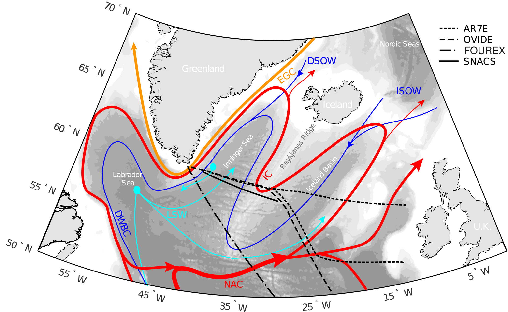
https://www.biogeosciences.net/15/51/2018/bg-15-51-2018-f01

Figure 1Schematic subpolar North Atlantic circulation. The location of the AR7E, OVIDE, FOUREX and SNACS lines are plotted in black on the bathymetry (500 m intervals). The branches of the North Atlantic Current (NAC) turning into the Irminger Current (IC) are shown in red and the East Greenland Current (EGC) is plotted in orange. The dark blue currents illustrate the spreading of the Iceland–Scotland Overflow Water (ISOW) and the Denmark Strait Overflow Water (DSOW) at depth, which jointly with the Labrador Sea Water (LSW), in cyan, contribute to the Deep Western Boundary Current (DWBC). Adapted from Lherminier et al. (2010) and Pérez et al. (2013).

Download

Over the past 3 decades, ocean CO₂ chemistry data have been collected on a regular basis in the world's oceans. As the observational record grows, direct evidence of the climate sensitivity of the marine carbon cycle emerges. For example, the Southern Ocean carbon sink exhibits clear variations in response to atmospheric circulation patterns; the sink was weakening from the early 1980s to the early 2000s (Le Quéré et al., 2007), but has strengthened in the more recent decades (Landschützer et al., 2015). In the subarctic western North Pacific, measurements from 1992 to 2008 at the two time series stations KNOT and K2 reveal decadal trends in total dissolved inorganic carbon (DIC) related to alkalinity-driven reductions in CO₂ outgassing (Wakita et al., 2010). In the Mediterranean Sea, changes in the large-scale circulation result in variability in the anthropogenic CO₂ concentration (Touratier and Goyet, 2009). Within the subpolar North Atlantic, high-quality carbon data have been collected almost every second year since the early 1990s (Olsen et al., 2016), enabling the determination of subdecadal variability. This shows relationships between the anthropogenic CO₂ storage rate and the extent and intensity of ventilation processes primarily driven by the North Atlantic Oscillation (NAO) (Fröb et al., 2016; Pérez et al., 2010; Wanninkhof et al., 2010; Woosley et al., 2016).

The subpolar North Atlantic is a key region for the storage and transport of CO₂ in the global ocean (Sabine et al., 2004). While a response of anthropogenic CO₂ storage to atmospheric forcing has been determined as mentioned above, less is known about variations in natural DIC, any relations to atmospheric forcing and relevance for total DIC inventories (Tanhua and Keeling, 2012). Here, we analyse changes in total DIC and its natural and anthropogenic components in the central subpolar North Atlantic, in the Irminger Sea, in relation to the distribution and evolution of water masses over a 24-year period from 1991 to 2015, covering three periods of variable convective activity (Fröb et al., 2016).

2 Hydrographic setting

The Irminger Sea, a central sea in the subpolar North Atlantic (Fig. 1), is a climatically sensitive area with strong hydrographic contrasts. The subpolar North Atlantic circulation pattern has been extensively presented in the literature; here the description follows Lavender et al. (2005) and Våge et al. (2011). In the upper ocean, the East Greenland Current carries cold and fresh water of Arctic origin southwards in the west close to the shelf of Greenland. In the east, the Irminger Current carries warm and salty water northwards along the Reykjanes Ridge. The salinity and temperature signature of these warm water masses is affected by the strength and shape of the subpolar gyre (Hátún et al., 2005; Häkkinen and Rhines , 2004). South of the Denmark Strait, they largely recirculate to the south. In the centre of the cyclonic circulation of the Irminger Gyre, preconditioning for convection is fulfilled (Bacon et al., 2003; Marshall and Schott, 1999; de Jong et al., 2012) and depending on heat loss, deep convection can occur (Fröb et al., 2016; Pickart et al., 2003 a; Våge et al., 2008, 2011; de Jong and de Steur, 2016). The extent and strength of convective processes are mainly driven by the state of the NAO, which is the leading mode of atmospheric variability over the mid-North Atlantic (Curry et al., 1998; Hurrell and Deser, 2009).

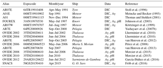
Stoll et al. (1996)Meincke and Becker (1993)Thomas and Ittekkot (2001)Johnson et al. (2003)Körtzinger et al. (1999)Yashayaev et al. (2007 b)Lherminier et al. (2010)Lherminier et al. (2010)van Heuven et al. (2012)Pérez et al. (2008)van Heuven et al. (2013)Mercier et al. (2015)Mercier et al. (2015)García-Ibáñez et al. (2016)Fröb et al. (2016)

Table 1Irminger Sea cruise information. The measured variables of the seawater CO₂ chemistry are indicated.

Download Print Version | Download XLSX

At depth, the circulation in the Irminger Sea is mainly characterized by the Denmark Strait Overflow Water (DSOW) and the Iceland–Scotland Overflow Water (ISOW). DSOW to the west is a relatively recently ventilated water mass enriched in oxygen (O₂) and other dissolved atmospheric gases. It is composed of several water masses originating from the Arctic Ocean and the Nordic Seas (Jeansson et al., 2008; Tanhua et al., 2005). ISOW originates from the intermediate waters of the Nordic Seas, which are modified as they flow through the Iceland Basin to the Irminger Sea (Hansen and Østerhus, 2000). In combination with ISOW and DSOW, Labrador Sea Water (LSW) forms North Atlantic Deep Water (NADW) (Dickson and Brown, 1994), the key component of the lower limb of the Atlantic Meridional Overturning Circulation. Two main LSW classes are identified in the subpolar North Atlantic: the LSW_1987−1994 and the LSW₂₀₀₀. LSW_1987−1994, from now on called classical LSW (cLSW), is a dense, cold and relatively fresh water mass with high concentrations of dissolved atmospheric gases formed by the recurring winter convection in the mid-1980s and mid-1990s in the Labrador and Irminger seas (Lazier et al., 2002; Pickart et al., 2003 b; Yashayaev et al., 2007 a). After 2000, the lighter LSW₂₀₀₀ or upper Labrador Sea Water (uLSW) has largely replaced cLSW (Yashayaev et al., 2007 b).

3 Data

Data from 15 cruises in the Irminger Sea covering 1991–2015 are used in this study (see Table 1). Data from the first 13 cruises were extracted from the GLODAPv2 data product, which provides bias-corrected, cruise-based, interior ocean data (Key et al., 2015; Olsen et al., 2016). The more recent data are from the 2012 OVIDE cruise (expocode: 29AH20120622) and the 2015 SNACS cruise (expocode: 58GS20150410). In order to minimize seasonal bias due to primary production, the upper 100 m of the water column are excluded from the inventory analysis. The region between 40.5 and 31.5^∘ W was covered by all 15 cruises.

All cruises intersect the ocean currents of the Irminger Sea described in the previous section. The cruises occupied either WOCE section A01/AR07E, the FOUREX or the OVIDE section, and locations are presented in Fig. 1. In order for the sections to be fully comparable, a coordinate transformation was performed for the 1997 FOUREX data. The latitude and longitude coordinates were rotated to the AR07E section using Cape Farewell as a pivot point. Adjusting the distance between the stations ensured that the adjusted coordinates of the station over the Reykjanes Ridge on the FOUREX line matched the station over the Reykjanes Ridge on the AR07E line. The inventory estimates are sensitive to depth, and therefore the pressure coordinates of all cruises were normalized. The location of every station for all cruises was mapped to the 1 arcmin global relief model of the Earth's surface (Amante and Eakins, 2009) using a nearest-neighbour interpolation. The ratio between the bottom depth of this bathymetry and the reported cruise station bottom depth was multiplied with the pressure coordinates of each station. This normalization step mainly affected the adjusted FOUREX data, while for the other cruises the normalization changed sampling depths by less than 20 m.

The accuracy of the GLODAPv2 data product is better than 0.005 in salinity, 1 % in O₂, 2 % in nitrate (NO₃), 2 % in silicate (SiO₂), 2 % in phosphate (PO₄), 4 µmol kg⁻¹ in DIC and 6 µmol kg⁻¹ in total alkalinity (A_T) (Olsen et al., 2016). For 29AH20120623, the overall accuracy of NO₃, PO₄ and SiO₂ was 1 %; the accuracy of DIC was 2 µmol kg⁻¹ and for A_T it was 4 µmol kg⁻¹ (García-Ibáñez et al., 2016; Ríos et al., 2015). For the SNACS cruise in 2015, pressure, conductivity, temperature and dissolved O₂ were directly measured with a Sea-Bird 911plus CTD profiler. At every station, water samples were obtained at 12 depths using Niskin bottles and used to calibrate the CTD measurements following the Global Ocean Ship-based Hydrographic Investigations Program (GO-SHIP) calibration procedure (Hood et al., 2010). The accuracy of bottle salinities analysed with a salinometer was ±0.003. The accuracy of O₂ concentrations measured with Winkler titration using a potassium iodate solution as a standard was 0.2 µmol kg⁻¹. The precision was better than 2 % in PO₄, 1 % in SiO₂ and 1 % in NO₃ as evaluated using samples drawn from sets of Niskin bottles tripped at the same depth. DIC and A_T were measured according to Dickson et al. (2007) with an accuracy of 2 µmol kg⁻¹ for both (Fröb et al., 2016).

The seawater CO₂ chemistry can be fully described if at least two of the four variables DIC, A_T, CO₂ partial pressure or pH are known. The measured variables at each of the 15 cruises are listed in Table 1. For six cruises, A_T and pH were measured, and therefore DIC was calculated for these using the dissociation constants of Lueker et al. (2000). For three cruises, only DIC was measured. For these, A_T was approximated using the salinity–alkalinity relationship for the North Atlantic from Lee et al. (2006). This relationship is defined for the surface ocean only, and therefore its validity for the deep Irminger Sea was tested (Appendix A). The mean difference between the approximated and the measured A_T data available was less than 5 µmol kg⁻¹; this is better than the target accuracy of A_T in the GLODAPv2 data product. No bias with depth or position was evident.

4 Method

The total DIC concentration is partitioned into its natural and anthropogenic components (DIC = DIC_nat + C_ant). The C_ant concentration was estimated with the φC_T^∘ method (see Sect. 4.1). The DIC_nat concentration is the difference between DIC and C_ant. For all cruises, the column inventories were estimated for DIC, DIC_nat and C_ant. The inventories are sensitive to depth, and therefore column inventories were only estimated for the part of the transect covered by all 15 cruises between 40.5 and 31.5^∘ W. The column inventory is the concentration profile integrated over the entire water column (Tanhua and Keeling, 2012):

\begin{matrix} (1) & {Inv}_{s} = \int_{0}^{z} c_{s} \cdot ϱ d z . \end{matrix}

Here, Inv_s is the column inventory of any species s, c_s its concentration, ϱ the density at in situ temperature and pressure and z the depth of the water column. The storage rate is the slope of a linear least-squares regression over the mean column inventories with time. The standard error of the slope is the error of the storage rate. Changes in inventories can be caused by changes in the distribution of water masses with different species concentrations or by changes in species concentration within the water masses. The distribution of water masses was determined using an extended optimum multiparameter analysis (eOMP; see Sect. 4.2). While the hydrographic parameters that describe a set of source water types (SWTs) used for the eOMP analysis are assumed to be time independent, the concentrations within each water mass of species such as DIC or C_ant vary over time and can therefore only be resolved by evoking the concept of water mass mixing-weighted average concentration, i.e. archetypal concentration (Álvarez-Salgado et al., 2013) (see Sect. 4.2). Finally, the inventory changes can be decomposed into contributions from changes in the archetypal concentration of the source water types and from changes in layer thickness of each water mass assuming linearity:

\begin{matrix} (2) & \frac{{dInv}_{tot}}{d t} = \sum_{WM} (\frac{\partial Inv}{\partial c} \frac{d c}{d t} + \frac{\partial Inv}{\partial z} \frac{d z}{d t}) . \end{matrix}

Here, $\frac{\partial Inv}{\partial c} \frac{d c}{d t}$ is the mean layer thicknesses with variable archetypal SWT concentrations, while $\frac{\partial Inv}{\partial z} \frac{d z}{d t}$ can be calculated as the mean archetypal SWT concentrations multiplied by the layer thickness changes over a specific time period. Hence, the two drivers of the observed inventory variability in total DIC and its natural and anthropogenic components can be identified.

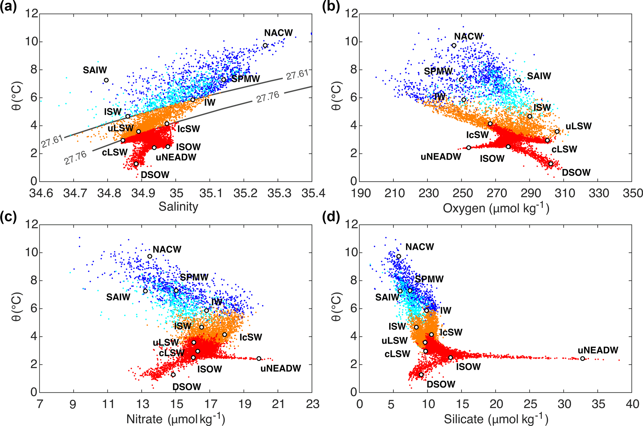
https://www.biogeosciences.net/15/51/2018/bg-15-51-2018-f02

Figure 2Source water type (SWT) parameters presented in a potential temperature: (a) salinity, including potential density (σ₀) levels, (b) oxygen, (c) nitrate and (d) silicate space for Irminger Sea cruise data from 1991–2015. The colours represent different mixing figures for the eOMP analysis: red for the deep ocean (σ₀ ≥ 27.76 kg m⁻³), orange for the intermediate ocean (27.61 ≤ σ₀ < 27.76 kg m⁻³) and surface ocean (σ₀ < 27.61 kg m⁻³), east of Reykjanes Ridge (dark blue) and west of Reykjanes Ridge region (cyan).

Download

4.1 Anthropogenic CO₂ calculation

The φC_T^∘ method was applied to all cruises in the Irminger Sea to estimate C_ant concentrations (Pérez et al., 2008; Vázquez-Rodríguez et al., 2009, 2012). The φC_T^∘ method is a back-calculation method that follows the same principles as the ΔC^* method of Gruber et al. (1996). In the φC_T^∘ method, C_ant is quantified as the difference between the preformed DIC at time t and at pre-industrial times (π): C_ant = DIC $^{^{\circ}, t}$ − DIC $^{^{\circ}, π}$ . DIC $^{^{\circ}, t}$ is calculated by correcting the measured DIC for changes due to the remineralization of organic matter and CaCO₃ dissolution, while DIC $^{^{\circ}, π}$ is quantified as the sum of the saturated DIC concentration with respect to the pre-industrial atmosphere and the air–sea CO₂ disequilibrium (ΔC_dis). The approach involves the following basic features: the subsurface layer (100–200 m) preserves conditions during water mass formation and is therefore taken as a reference. ΔC_dis is parameterized based on subsurface data using a short-cut approach to calculate C_ant. The set of parameterizations for preformed alkalinity (A_T^∘) and ΔC_dis obtained from the subsurface data are applied directly to waters with temperatures larger than 5^∘ C. For waters below the 5^∘ C isotherm, A_T^∘ and ΔC_dis estimates are based on an eOMP analysis, which was successfully used in previous studies (Pérez et al., 2008; Vázquez-Rodríguez et al., 2009, 2012). This eOMP determines in each sampling point the fraction of six water masses that ventilate the global ocean, taking different formation histories and water mass origins into account. Each water mass has assigned values for A_T^∘ and ΔC_dis and together with the obtained fractions, A_T^∘ and ΔC_dis are calculated. Note that this eOMP analysis is only used to determine A_T^∘ and ΔC_dis, which are used in the C_ant calculation. This is independent of the eOMP set-up for the Irminger Sea water mass analysis (see Sect. 4.2).

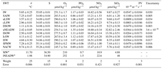
Table 2Source water type (SWT) parameters and their standard deviation used for the eOMP analysis for Subarctic Intermediate Water (SAIW), Intermediate Water (IW), classical and upper Labrador Sea Water (cLSW and uLSW), Denmark Strait Overflow Water (DSOW), upper North-east Atlantic Deep Water (uNEADW), Iceland–Scotland Overflow Water (ISOW), Icelandic Slope Water (IcSW), Irminger Sea Water (ISW), Subpolar Mode Water (SPMW) and North Atlantic Central Water (NACW). Definitions for Mediterranean Water (MW) and lower North-east Atlantic Deep Water (lNEADW) (^*) from García-Ibáñez et al. (2015) are used only for the composite analysis but not in the eOMP. The weights for the equations are given. The mass weight is 150. The mean parameter residual is given (error). The last column gives an uncertainty estimate (per one) for the SWT contribution based on a Monte Carlo simulation.

Download Print Version | Download XLSX

The major advantage of the φC_T^∘ method over other back-calculation methods is that it does not rely on measurements of age tracers, such as chlorofluorocarbons (CFCs). Further, the parameterized A_T^∘ is corrected for effects of CaCO₃ dissolution changes and the sea surface temperature increase since pre-industrial times and any spatial and temporal variability in ΔC_dis is taken into account. Overall, the uncertainty of φC_T^∘-derived C_ant has been reported to be 5 µmol kg⁻¹ (Pérez et al., 2008; Vázquez-Rodríguez et al., 2009).

4.2 Extended optimum multiparameter analysis (eOMP)

The optimum multiparameter (OMP) analysis (Tomczak and Large, 1989) is used to estimate the contribution of water masses, which are represented through SWTs, to each water parcel along the Irminger Sea sections. The OMP analysis assumes that all hydrographic parameters describing the water masses are affected by the same mixing processes. For each sampling point the contribution of the various water masses is quantified from an over-determined system of linear mixing equations, which is solved in a non-negative least-squares sense assuming that the parameters are linearly independent:

\begin{matrix} (3) & G x - d = Res, \end{matrix}

where G is the SWT matrix containing their properties, x the relative contributions of each SWT to the sample, d the observed data and Res the residual, which is minimized in the calculation. The OMP was further developed into the extended OMP (eOMP) analysis by Karstensen and Tomczak (1998); in the present analysis an eOMP has been adopted. This accounts for the non-conservative behaviour of O₂ and nutrients by using Redfield ratios. In the eOMP, the remineralization of NO₃ and PO₄ is numerically related to an oxygen consumption rate, which, if multiplied with a pseudo-age, is similar to apparent oxygen utilization (AOU) (Poole and Tomczak, 1999). OMP and eOMP analyses have previously been used to describe in detail the origin, pathways and transformation of the main water masses in the subpolar North Atlantic (García-Ibáñez et al., 2015; Tanhua et al., 2005; Álvarez et al., 2005). Here, the SWT properties were defined based on the cruise data from 1991, assuming that the properties of the SWTs do not significantly change over time. The data for potential temperature (θ), salinity, O₂, NO₃, PO₄, SiO₂ and potential vorticity (PV) were used to characterize 11 SWTs that combined encompass the property features in the Irminger Sea (Fig. 2), namely Subarctic Intermediate Water (SAIW), Intermediate Water (IW), classical and upper Labrador Sea Water (cLSW and uLSW), Denmark Strait Overflow Water (DSOW), upper North-east Atlantic Deep Water (uNEADW), Iceland–Scotland Overflow Water (ISOW), Icelandic Slope Water (IcSW), Irminger Sea Water (ISW), Subpolar Mode Water (SPMW) and North Atlantic Central Water (NACW). The properties of the SWTs are provided in Table 2, including their standard deviations. These values were determined from the 10 % of data in the relevant density class that were closest to the property maximum or minimum used to delineate the SWT. For example, if an SWT was defined as a salinity minimum, all data points within a specific potential density (σ) range were sorted by salinity and the mean and standard deviation over the first 10 % of the data points gave the salinity properties for that SWT. The approximate locations of all SWTs are shown in Fig. 3.

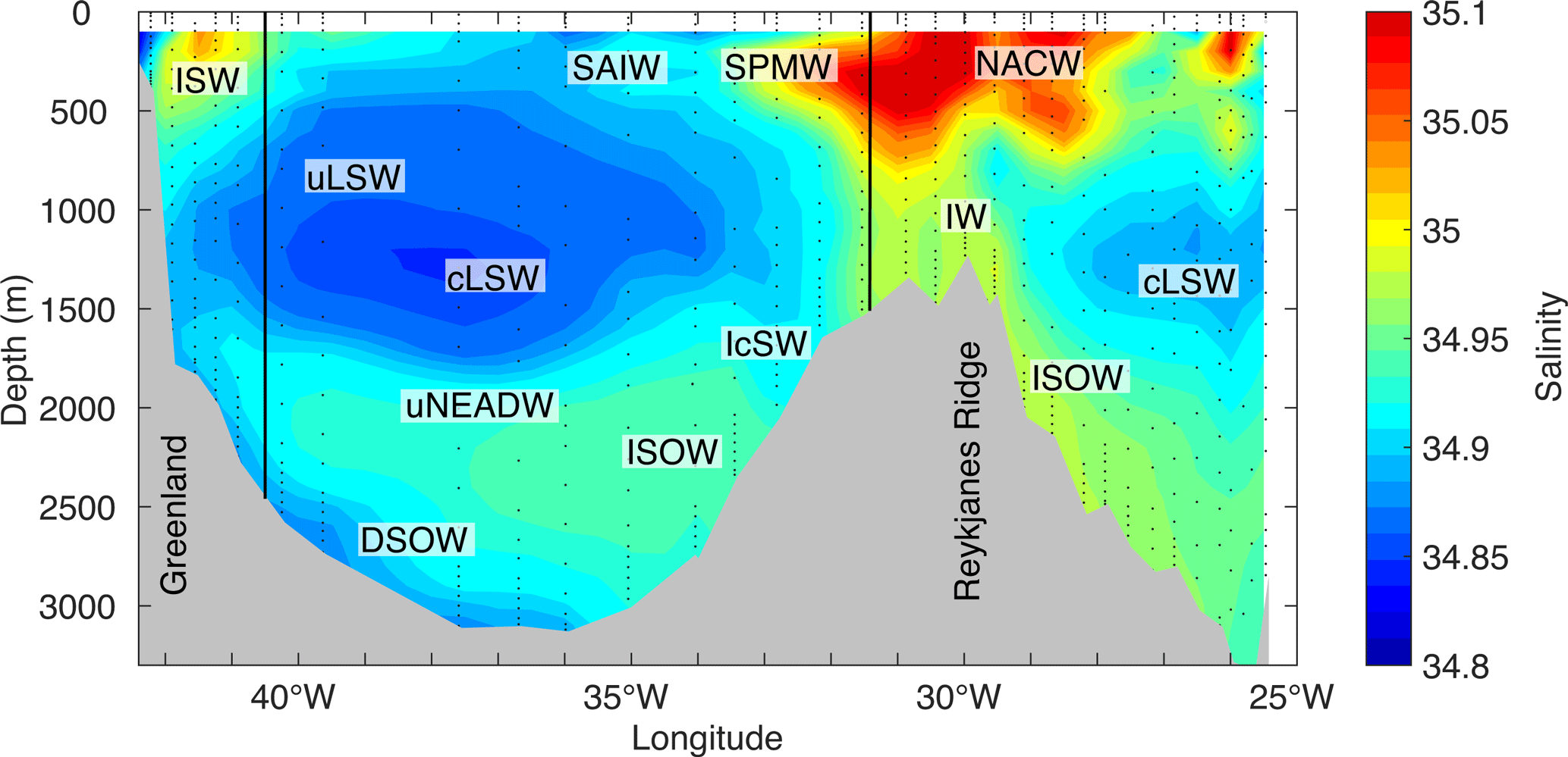
https://www.biogeosciences.net/15/51/2018/bg-15-51-2018-f03

Figure 3Vertical cross section through the Irminger Sea showing interpolated salinity based on the 1991 cruise data (06MT19910902). The approximate location of the main water masses of the eOMP analysis, explicitly shown in Appendix B, is illustrated: Subarctic Intermediate Water (SAIW), Intermediate Water (IW), classical and upper Labrador Sea Water (cLSW and uLSW), Denmark Strait Overflow Water (DSOW), upper North-east Atlantic Deep Water (uNEADW), Iceland–Scotland Overflow Water (ISOW), Icelandic Slope Water (IcSW), Irminger Sea Water (ISW), Subpolar Mode Water (SPMW), North Atlantic Central Water (NACW). The longitudinal boundaries for the inventory estimates at 40.5 and 31.5^∘ W are shown (black lines).

Download

DSOW is the densest water mass in the Irminger Sea and defined as an O₂ maximum at σ₂ levels denser than 37.10 kg m⁻³ (Yashayaev et al., 2007 b). ISOW is defined as a salinity maximum between 36.89 and 37.10 kg m⁻³ (σ₂) and θ between 2.3 and 2.6 ^∘C. North-east Atlantic Deep Water (NEADW) is formed by the entrainment of ISOW with surrounding waters, mainly deep water of Antarctic origin. In the North Atlantic, two classes have been identified: upper and lower NEADW (uNEADW and lNEADW) (Castro et al., 1998). However, in the Irminger Sea lNEADW is non-existent (McCartney, 1992), while uNEADW was identified as a maximum in SiO₂ below 2500 m. The mid-depth weakly stratified layer of cLSW in the Irminger Sea was identified by a PV and salinity minimum between 36.90 and 36.94 kg m⁻³ (σ₂); uLSW is less dense than cLSW due to its slightly different θ salinity signature and was identified as a minimum in PV in the 36.81–36.87 kg m⁻³ σ₂ range.

The Icelandic Slope Water (IcSW), the Intermediate Water (IW), the Irminger Sea Water (ISW) and the uLSW are typically found at intermediate depths. IcSW is a warm and saline water mass close the Reykjanes Ridge on the Iceland slope (Tanhua et al., 2005; Yashayaev et al., 2007 a). Here, IcSW was defined by a minimum in O₂ occupying the 36.80–36.86 kg m⁻³ σ₂ range, effectively separating uLSW and cLSW. IW is a saline water mass depleted in O₂ and of southern origin (Sarafanov et al., 2008). IW was identified by O₂ values below 250 µmol kg⁻¹ at σ₀ between 27.45 and 27.65 kg m⁻³. ISW is fresh, elevated in O₂ and found between 4 and 5 ^∘C.

Finally the Subpolar Mode Water (SPMW), the Subarctic Intermediate Water (SAIW) and the North Atlantic Central Water (NACW) are all typically found in the upper Irminger Sea. SPMW is oxygenated and of subpolar origin. It was defined as a salinity maximum in the 7–8 ^∘C θ range. SAIW is a salinity minimum in the 6.5–7.5 ^∘C θ range. NACW was defined as the salinity maximum for θ above 9 ^∘C.

The seven hydrographic parameters describing the SWTs limit the number of SWTs included in one eOMP analysis to a maximum of seven. In addition, the required mass conservation over-determines the system of linear equations. However, NO₃ and PO₄ might be locally correlated, and therefore 1 degree of freedom for the eOMP analysis is potentially lost. Therefore, the Irminger Sea was divided into four regions, defined such that each contained a maximum number of five SWTs to be determined with the seven parameters plus mass conservation. This ensures the over-determination of the system of mixing equations, which can then be solved. In the deep ocean (σ₀ ≥ 27.76 kg m⁻³), SWTs were limited to DSOW, ISOW, uNEADW, cLSW and IcSW. In the intermediate ocean (27.61 ≤ σ₀ < 27.76 kg m⁻³), only ISW, IW, IcSW, uLSW and cLSW were included. The upper ocean (σ₀ < 27.61 kg m⁻³) was split into two basins: east of Reykjanes Ridge (NACW, SPMW, IW and SAIW) and west of the Reykjanes Ridge (ISW, SPMW, IW and SAIW). The data presented in Fig. 2 are classified according to these “mixing figures”. While the density boundaries were used to identify the set of SWTs potentially present, the eOMP analyses were performed at each sampling point. The equations were normalized and weighted, accounting for differences in measurement accuracies and potential environmental variability. Weights were assigned according to the variability and accuracy of the parameters following García-Ibáñez et al. (2015). The highest weight was assigned to mass to ensure its conservation. The second highest weights were assigned to θ and salinity because they are the most accurate. PV was weighted high as well due to its good accuracy and to enable the resolution of both LSW classes. The eOMP results in a ratio r_ij; this describes the contribution of each SWT, i, to each data point in space and time, j.

In order to determine SWT concentrations of time-varying species such as DIC, DIC_nat and C_ant, the mixing-weighted concentration or archetypal concentration, C_i, of these species was calculated for each SWT, i (Álvarez-Salgado et al., 2013):

\begin{matrix} (4) & C_{i} = \frac{\sum_{j} r_{i j} \times C_{j}}{\sum_{j} r_{i j}} . \end{matrix}

Here, the concentration in each sampling point j, C_j, is multiplied with the ratio of the SWT in that point r_ij. When summed over all points and divided by the total fraction the SWT occupies, this estimates C_i. Further, the layer thickness, Th, of each SWT at each station is estimated according to

\begin{matrix} (5) & {Th}_{i k} = \frac{\sum_{j} r_{i j}}{n_{k}} \times d_{k, \max} . \end{matrix}

Here, $\frac{\sum_{j} r_{i j}}{n_{k}}$ is the fraction of the total water column that each SWT occupies at each station, with n_k describing the number of sampling points per station. The fraction is unitless and needs to be scaled to the total water column height, i.e. multiplied by the maximum depth of the station, d_k,max. The average layer thickness over all stations of the Irminger Sea transect is the mean layer thickness. As each water parcel is a mixture of different water masses represented by r_ij, Eq. (5) allows us to convert each composite to a measure of height.

4.3 Uncertainty analysis

Uncertainties for the distribution of water masses result from measurement uncertainties and errors in the eOMP analysis. Here, the largest source of error is the definition of the SWTs. The SWT matrix needs to represent the known features of the circulation (Tanhua et al., 2005), but temporal shifts in SWT characteristics cannot be accounted for with the eOMP analysis. A measure of uncertainty is given by the difference between measured and eOMP-calculated values, the residual Res in Eq. (3). The total residual, calculated by taking the square of the largest parameter residual at each sampling point (García-Ibáñez et al., 2015), and the individual parameter residuals are shown in Fig. 4. Below 1200 m, the total residual is close to zero, as are the residuals of θ, salinity and O₂. In the intermediate and surface ocean these residuals increase, particularly for O₂, which might be a consequence of gas exchange. The residuals of PO₄, NO₃ and SiO₂ are larger, as expected due to their lower weights in the eOMP, and do not show any trend with depth. The mean error for each parameter is listed in Table 2. These are of similar magnitude as the errors determined for the Irminger Sea eOMP analysis by Tanhua et al. (2005).

In order to test how robust the results of the eOMP analysis are, a Monte Carlo simulation was performed (Tanhua et al., 2005). The properties of the SWT matrix were randomly perturbed within the standard deviation of each parameter; 100 of such perturbed SWT matrices were created and the eOMP was solved for each perturbed system. This allows for the quantification of the sensitivity of the eOMP to potential temporal variations i the SWT properties. The standard deviation of the mean SWT contribution over all 100 perturbations is shown in the last column of Table 2. The uncertainties are generally low, and hence the robustness of the eOMP analysis is high.

https://www.biogeosciences.net/15/51/2018/bg-15-51-2018-f04

Figure 4Residuals of the eOMP analysis for all Irminger Sea cruise data from 1991–2015 for the (a) total residual as the squared largest singular value for the set of residuals (García-Ibáñez et al., 2015) and the residual of mass conservation in %, (b) residuals of potential temperature and salinity, (c) residuals of phosphate and nitrate and (d) residuals of oxygen and silicate with respect to pressure.

Download

The layer thickness uncertainties were estimated by scaling the averaged standard deviation of each SWT, which were quantified with the Monte Carlo simulation, to the width and depth of the Irminger Sea. The uncertainty of C_ant concentrations is 5 µmol kg⁻¹, and for DIC and DIC_nat it is 4 µmol kg⁻¹. Errors for the inventories were estimated by propagating the uncertainties of the layer thicknesses and the concentrations through the water column.

5 Results

Over the 24-year period considered here, the frequency and the amplitude of the mean winter NAO changed significantly (Hurrell and Deser, 2009). The convection in the subpolar gyre during winter, which is driven by the large-scale atmospheric circulation (Lazier et al., 2002; Pickart et al., 2003 b; Yashayaev et al., 2007 a), has varied in strength and extent accordingly. Three distinctive time periods can be characterized from 1991 to 2015 by different levels of convective activity in the Irminger Sea. In the first period from 1991 to 1997, several consecutive positive NAO winters led to extensive deep convection in the entire subpolar gyre (Pickart et al., 2003 a, b). In the second period from 2000 to 2007, the NAO was in a more neutral state and only shallow convection occurred in the Irminger Sea. In the third period from 2008 to 2015, three deep convective events took place in the Irminger Sea in 2008, 2012 and 2015 (Fröb et al., 2016; Våge et al., 2008; de Jong and de Steur, 2016; de Jong et al., 2012). The DIC, DIC_nat and C_ant inventory changes are presented with respect to these three periods and for the entire 24 years of observations in the following sections.

The temporal change in DIC, DIC_nat and C_ant concentration in the Irminger Sea is clearly visible in Fig. 5, which shows interpolated cruise station data for 1991, 1997, 2007 and 2015 as the start and end years of the three periods considered here. The increase in DIC is evident throughout the basin. From 1991–1997, cLSW with a low DIC signature dominates the basin, but a tongue of older IW over the Reykjanes Ridge transports relatively high DIC concentrations into the Irminger Sea. By 2015 the DIC concentration had increased by at least 10 µmol kg⁻¹ compared to 1991, as visualized by the disappearance of the 2150 µmol kg⁻¹ contour line (Fig. 5a). Temporal changes in DIC_nat concentration (Fig. 5b) are small compared to those in DIC and less systematic. The C_ant concentration increases over time, not only at the surface, but also over the entire water column, which is indicated by the disappearance of the 20 µmol kg⁻¹ contour line below 1500 m from 1991 to 2015 (Fig. 5c).

https://www.biogeosciences.net/15/51/2018/bg-15-51-2018-f05

Figure 5Vertical cross sections through the Irminger Sea showing interpolated cruise station data of (a) DIC, (b) DIC_nat and (c) C_ant concentration in 1991 (first column), 1997 (second column), 2007 (third column) and 2015 (last column). The white contour lines illustrate selected concentration levels. All panels have the same span of values of 40 µmol kg⁻¹.

Download

https://www.biogeosciences.net/15/51/2018/bg-15-51-2018-f06

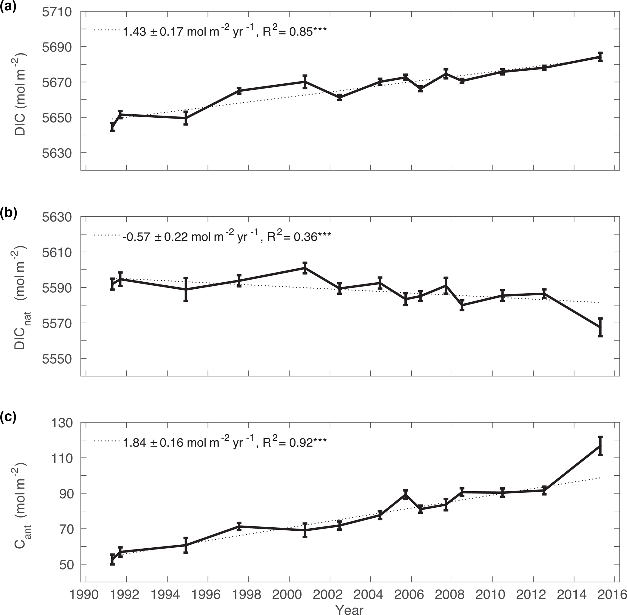
Figure 6Total inventory for (a) DIC, (b) DIC_nat and (c) C_ant for Irminger Sea cruise data from 1991–2015. The rates of change between 1991 and 2015 are given, including the R-squared value of the linear regression model. Significance at the 99 % level ( $^{* * *}$ ) is indicated. Values of the two cruises in 1997 were averaged and are shown as one data point.

Download

https://www.biogeosciences.net/15/51/2018/bg-15-51-2018-f07

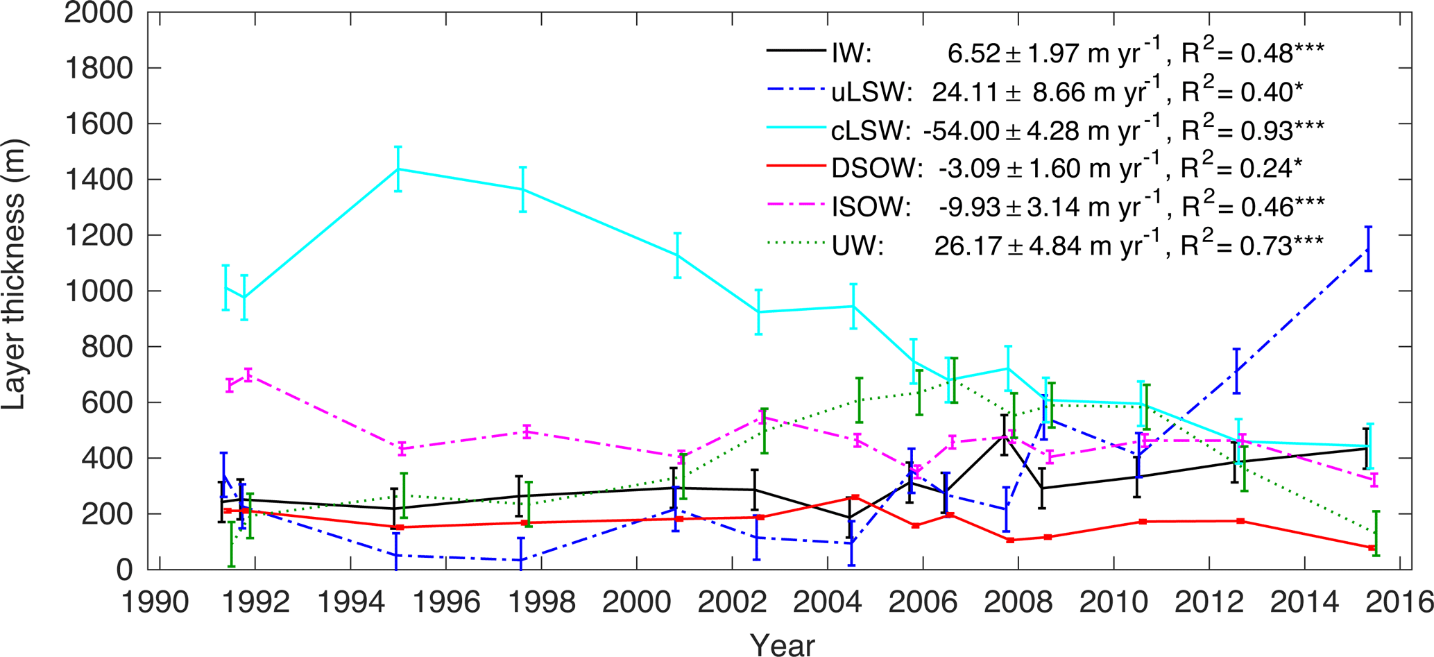
Figure 7Layer thickness for IW, uLSW, cLSW, DSOW, ISOW and the sum over the upper ocean waters (UWs) based on Irminger Sea cruise data from 1991–2015. The mean depth between 40.5 and 31.5^∘ W is 2650 m. The error bars show the uncertainty based on a Monte Carlo simulation scaled to the width and depth of the Irminger Sea. The rates of thickness change between 1991 and 2015 are given for all SWTs, including the R-squared value of the linear regression model. Significance at the 90 % level (^*) or the 99 % level ( $^{* * *}$ ) is indicated. Values of the two cruises in 1997 were averaged and are shown as one data point. All markers are slightly offset in time for clarity.

Download

The column inventory time series of DIC, DIC_nat and C_ant shown in Fig. 6 quantifies this large temporal change in the Irminger Sea sections. Typically, the DIC inventory increased by 1.43 ± 0.17 mol m⁻² yr⁻¹ from 1991 to 2015, from approximately 5645 to 5685 mol m⁻². The C_ant storage rate was 1.84 ± 0.16 mol m⁻² yr⁻¹ in the same time period, which is larger than the rate of DIC inventory change. At the same time, the DIC_nat inventory decreased at a rate of −0.57 ± 0.22 mol m⁻² yr⁻¹. Therefore, the annual change in the DIC inventory is mainly driven by the large C_ant storage rate but partially offset by the loss in DIC_nat inventory. The variability in the DIC and C_ant inventories over the 24-year period is of similar magnitude, as indicated by the error of the slope in Fig. 6, whereas the DIC_nat inventory varies slightly more. DIC_nat increases as water masses age and DIC_nat from the remineralization of organic matter accumulates, while it decreases during water mass renewal and/or ventilation, which brings water with preformed, relatively low DIC_nat concentrations into the ocean interior. It is notable that the C_ant inventory increased sharply from 2012 to 2015, while there was a comparably large decline in the DIC_nat inventory. This is not an artefact of the method, but can be explained by the fact that the 2015 data were obtained during active convection in the Irminger Sea (Fröb et al., 2016). During the strong convection, older water masses enriched in DIC_nat were replaced by water masses high in C_ant due to their most recent contact to the atmosphere and relatively low in DIC_nat as DIC_nat from remineralization has not yet accumulated. In contrast to that, the peak in 2005 in the C_ant inventory could be related to the advection of C_ant-enriched water masses formed in the Labrador Sea or in the region south of Cape Farewell into the Irminger Sea (Palter et al., 2016; Straneo et al., 2003), but this strong signal may also reflect the true error or reveal measurement bias.

5.1 SWT distribution

The layer thickness of the Irminger Sea SWTs from 1991 to 2015 is presented in Fig. 7. Because their individual contributions are small, the upper ocean SWTs, i.e. NACW, ISW and SPMW, are combined and titled upper waters (UWs). For reasons of simplicity, the number of SWTs were reduced from 11 to 9 by performing composite analyses for uNEADW and IcSW. The uNEADW was determined to be a composite of 26 % ISOW, 14 % LSW, 58 % lNEADW and 2 % Mediterranean Water (MW) based on salinity, θ and SiO₂ following van Aken (2000). Properties for the SWTs representing lNEADW and MW were taken from García-Ibáñez et al. (2015). A decomposition based on salinity and θ showed that IcSW is a composite of 30 % ISOW, 20 % cLSW and 50 % IW. Based on the composite analysis, the contributions of uNEADW and IcSW are divided up and added to cLSW, IW and ISOW. MW and lNEADW only appear in the Iceland Basin and are not included for further analysis. Therefore, not all 11 SWTs used for the eOMP analysis are shown, but only UW, IW, uLSW, cLSW, DSOW and ISOW. Since the FOUREX section occupied in 1997 was located further south than the AR07E section, which was covered that year by 06MT19970707, the SWT distribution differs slightly between the two cruises. At the FOUREX section, the ISOW layer is on average 50 m and the SAIW layer is about 15 m thicker than further north, while the ISW layer is about 47 m and the SPMW layer is 19 m thicker for 06MT19970707 than at the FOUREX section. For the other SWTs, differences are smaller than 8 m. Relatively speaking, 50 m is less than 2 % of the entire water column, so the discrepancy between the two cruises is small compared to the mean depth of the Irminger Sea.

Table 3Mean layer thickness and concentration of DIC, DIC_nat and C_ant in IW, uLSW, cLSW, DSOW, ISOW and UW in the time periods from 1991–2015, 1991–1997, 2000–2007 and 2008–2015.

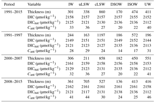
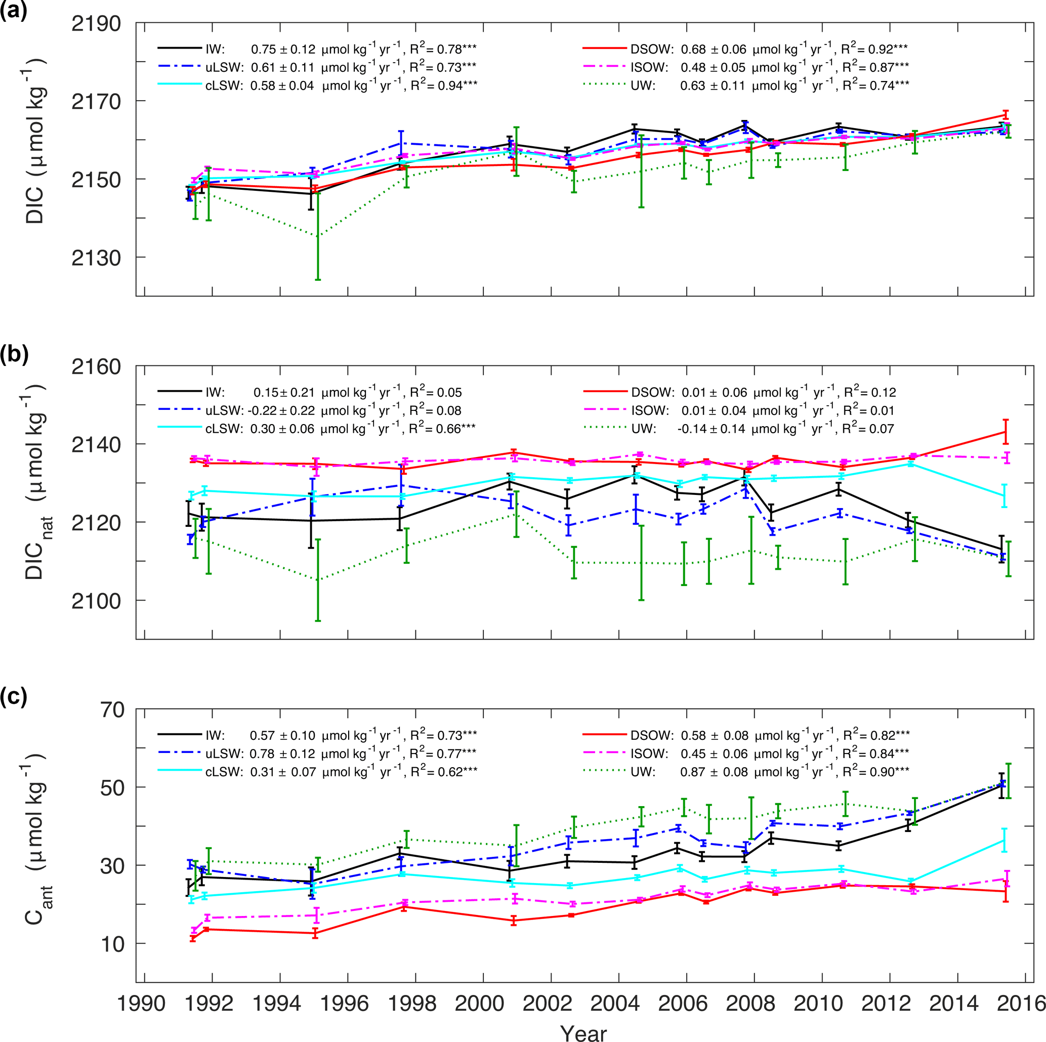
Download Print Version | Download XLSX

https://www.biogeosciences.net/15/51/2018/bg-15-51-2018-f08

Figure 8Archetypal concentration for IW, uLSW, cLSW, DSOW, ISOW and the sum over the upper ocean waters (UWs) in the Irminger Sea from 1991 to 2015 for (a) DIC, (b) DIC_nat and (c) C_ant. The error bars represent σ. The storage rates between 1991 and 2015 are given for all SWTs, including the R-squared value of the linear regression model. Significance at the 90 % level (^*) or the 99 % level ( $^{* * *}$ ) is indicated. Values of the two cruises in 1997 were averaged and are shown as one data point. All markers are slightly offset in time for clarity.

Download

The distribution of SWTs in the Irminger Sea, as shown in Fig. 7, changes substantially from 1991 to 2015. The overall trend is indicated, but the rates of change are often larger if sub-periods are considered. For example, the IW layer thickens slightly from 1991 to 2015 at a rate of 6.5 ± 2.0 m yr⁻¹, but there is little change before 2004, while after 2004 the layer thickness increase is much stronger. The uLSW layer thickness increases by an average of 24.1 ± 8.7 m yr⁻¹, but it is very thin before 1997 and the major build-up occurs after 2004. In particular, after deep convection in the Irminger Sea in 2008, 2012 and 2015, the layer thickness of uLSW increases substantially. The cLSW layer shows the largest changes in thickness at a loss rate of −54.0 ± 4.3 m yr⁻¹ from 1991 to 2015. The convective activity in the subpolar gyre from 1991 to 1997 led to the extensive production of cLSW. After that, the cLSW layer was not renewed and strongly diminished until 2015. In contrast to that, the DSOW layer decreases little in thickness over the 24-year period covered by the data. The ISOW layer thins by −9.9 ± 3.1 m yr⁻¹. Over the entire period from 1991 to 2015 the UW layer thickness increases at a rate of 26.2 ± 4.8 m yr⁻¹, but it essentially has a constant thickness from 1991 to 2000, then thickens until 2007 and decreases in thickness after that. Overall, the change in the distribution of the main SWTs is well captured by the eOMP analysis. The transformation of the two LSW classes particularly seems to match the observations well (Yashayaev et al., 2007 a).

The mean layer thickness for each SWT in the time periods considered here is summarized in Table 3. The main variability in the distribution of water masses is created by layer thickness changes of cLSW, uLSW and UW. With only small changes over the 24-year period, DSOW, ISOW and IW occupy a little more than one-third of the Irminger Sea sections. In the mid-1990s, the cLSW layer occupied close to 50 % of the entire water column, which left thin uLSW and UW layers corresponding to less than 7 % and around 8 %, respectively, of the entire water column. As cLSW was advected out of the Irminger Sea while not being re-formed by convection, that layer was replaced mainly by UW in the early 2000s. In 2004, cLSW occupied 37 % of the water column and UW occupied 24 %, while the uLSW layer only accounted for 4 %. With the recurring convection events between 2008 and 2015, uLSW was formed more frequently and displaced UW and the remainder of the cLSW layer. The measurements from winter 2015 reveal that by then the fraction of cLSW was as low as 17 % and that of UW was only 5 %, but uLSW occupied 45 % of the entire water column.

5.2 Archetypal concentration changes

Within the SWTs, the archetypal concentrations of carbon species change over time due to the remineralization of organic matter, for example, which adds DIC_nat, or air–sea gas exchange, which increases C_ant in water masses that are in contact with the atmosphere. The archetypal concentrations of DIC, DIC_nat and C_ant from 1991 to 2015 are shown in Fig. 8 for the same SWTs as in Fig. 7 and are also summarized in Table 3. In all SWTs, DIC is similar except for UWs, which have a more variable DIC that is generally lower compared to all other SWTs. The older SWTs in the deep ocean have higher DIC_nat concentrations and lower C_ant concentrations compared to SWTs that have been ventilated more recently. Therefore, the deep SWTs, namely ISOW and DSOW, have the highest archetypal concentrations of DIC_nat (both 2136 µmol kg⁻¹) and the lowest archetypal concentrations of C_ant (22 and 20 µmol kg⁻¹), respectively. In contrast, UWs have the lowest archetypal concentrations of DIC_nat (2112 µmol kg⁻¹) and the highest archetypal concentrations of C_ant (40 µmol kg⁻¹), which are almost twice as high as in the deep SWTs.

For all SWTs, the rate of change in the archetypal DIC concentration is similar except for ISOW in which it is slightly smaller. The archetypal concentration change over time for DIC_nat is not statistically different from zero for most SWTs apart from cLSW in which the DIC_nat concentration increases by 0.30 ± 0.06 µmol kg⁻¹ yr⁻¹. In contrast, the archetypal C_ant concentration increases significantly in all SWTs over time. Further, the increase rate of the archetypal DIC concentration is not statistically different from the rate of increase of the archetypal C_ant concentration. This indicates that the increase in DIC can be explained by the input of C_ant to the entire water column. This is true for all SWTs except cLSW. For this water mass the increase in the archetypal C_ant concentration contributes 0.31 ± 0.07 µmol kg⁻¹ yr⁻¹ to the increase in DIC, which is only half of the DIC concentration increase. This is because DIC_nat accumulates as cLSW ages, while at the same time, a smaller fraction of C_ant is added to this water mass due to less frequent ventilation.

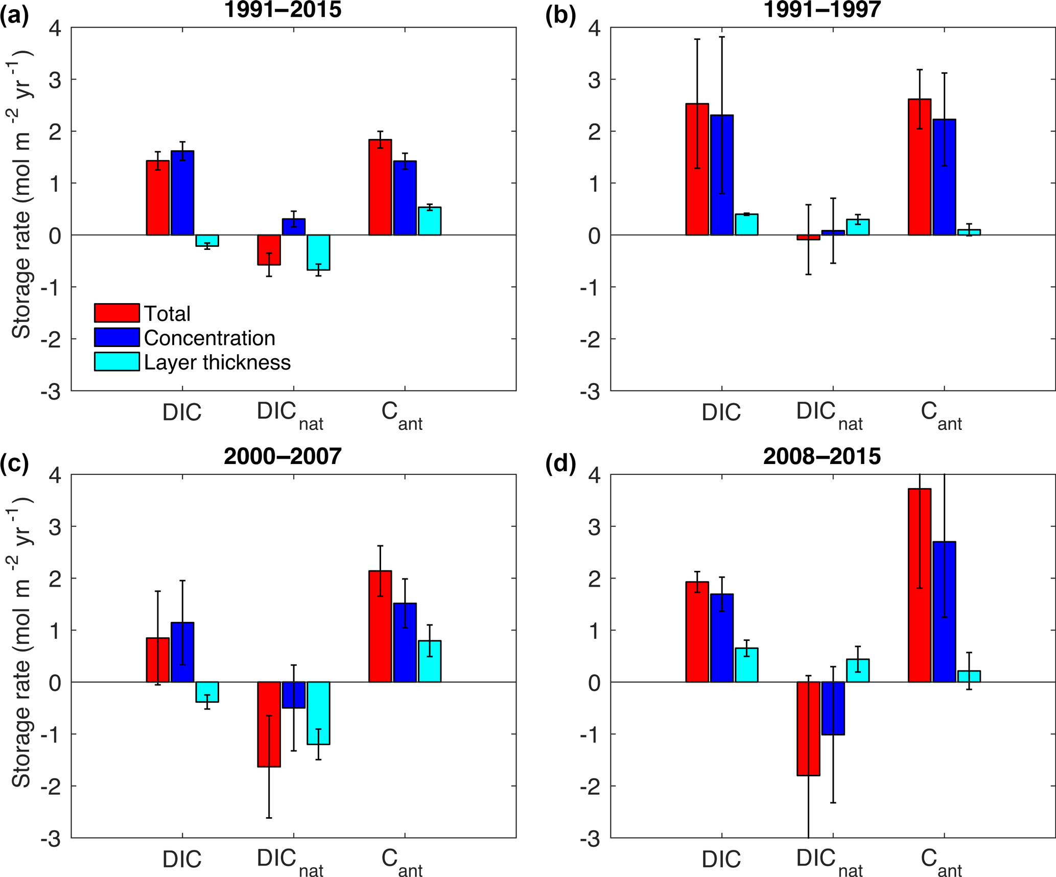
https://www.biogeosciences.net/15/51/2018/bg-15-51-2018-f09

Figure 9Decomposition of the total storage rates (red bars) into the concentration-driven storage rate (blue bars) and the layer-thickness-driven storage rate (cyan bars) for DIC, C_ant and DIC_nat from (a) 1991–2015, (b) 1991–1997, (c) 2000–2007 and (d) 2008–2015. The error bars represent the error of the linear regression model.

Download

5.3 DIC storage rate decomposition

The decomposition of the inventory changes reveals the contribution that changes in the SWT distribution and changes in the concentration within these SWTs have on the total storage rate of DIC and its natural and anthropogenic components. Figure 9 summarizes the storage rates of DIC, DIC_nat and C_ant over the entire 24-year time period and for the periods 1991–1997, 2000–2007 and 2008–2015. The first bar shows the total storage rate summed over all SWTs. The second bar shows the concentration-driven storage rate, and the third bar shows the layer-thickness-driven storage rate. In theory, the first bar should be the sum of the last two bars. However, since the storage rates have been calculated using a linear regression over only a small number of data points, the residuals can become quite large; this is especially the case for shorter time periods. Nevertheless, some conclusions can be drawn. The increase in the DIC inventory from 1991 to 2015 is driven by the increase in the C_ant inventory and partially offset by a decrease in DIC_nat inventory. The rise in the C_ant inventory is primarily due to a rise in C_ant concentration, but the contribution from layer-thickness-driven changes is also significantly positive (Fig. 9a). While the rise in C_ant concentration occurs in all SWTs (Fig. 8), the contribution from the latter factor appears mostly driven by the increase in the thickness of uLSW (Fig. 7), which is rich in C_ant (Fig. 8). The decrease in the DIC_nat inventory is the result of the layer-thickness-driven reduction, which is larger than the concentration-driven increase (Fig. 9a). This can be attributed to the replacement of cLSW with uLSW and UW, which both have lower concentrations of DIC_nat.

The variations at subdecadal timescales can be understood in terms of the convective activity in the Irminger Sea, although with larger uncertainty. Figure 9b shows the decomposed trends from 1991–1997, a period when convective activity was high in the subpolar gyre. The total DIC storage rate is driven by the C_ant storage rate, while the changes in the DIC_nat inventory are not significantly different from zero. The C_ant storage rate is mainly driven by increasing concentrations, which occur in all SWTs (Fig. 8).

From 2000–2007, although the C_ant storage rate of 2.14 ± 0.49 mol m⁻² yr⁻¹ was similar to that of the preceding period, the DIC storage rate was much smaller because of the large loss of DIC_nat. The 2000–2007 period has the smallest DIC storage rate of all periods considered, 0.65 ± 0.39 mol m⁻² yr⁻¹, compared to 2.53 ± 1.24 and 1.93 ± 0.20 mol m⁻² yr⁻¹ for the earlier and later periods, respectively. Also, unlike the other periods, changes in layer thickness and concentrations were almost equally important for the C_ant storage rate. The DIC_nat storage rate, on the other hand, was almost entirely driven by changes in layer thickness: −1.20 ± 0.29 mol m⁻² yr⁻¹ of a total of −1.63 ± 0.98 mol m⁻² yr⁻¹. From Figs. 7 and 8 these features appear to be the result of uLSW and UW replacing cLSW. Their larger concentrations of C_ant leads to the relatively large layer-thickness-driven storage increase, while the advection of DIC_nat-rich cLSW out of the Irminger Sea leads to the negative layer-thickness-driven decrease in the DIC_nat inventory. The negative concentration-driven storage rate appears primarily driven by the loss of DIC_nat from uLSW and UW outweighing the increase in DIC_nat in the cLSW.

For the last period from 2008–2015 (Fig. 9d), the deep convection in 2015 had a large impact on all storage rates and their uncertainty estimates; i.e. the exceptional changes in 2015 incur large uncertainty on the regression slopes for this time period. The DIC storage rate is 1.93 ± 0.20 mol m⁻² yr⁻¹ and the result of a large C_ant storage rate, the largest in all three periods considered, offset by a negative DIC_nat storage rate. Both of these are primarily the result of changes in concentrations indicative of the ventilation that occurred. As evaluated from Fig. 8, the C_ant increase is greatest in IW, uLSW and UW, while the loss of DIC_nat occurred primarily in the IW and uLSW. However, cLSW also appears to be affected by the most recent event in 2015.

6 Discussion

The data that have been collected in the Irminger Sea over the past decades provide unequivocal evidence for climate forcing of the carbon cycle in this oceanic region. Over long timescales, the steady trend due to the uptake of anthropogenic CO₂ clearly dominates, but at shorter timescales it varies and can also be significantly masked by variability in DIC_nat. In particular, this was the case in the period from 2000 to 2007 when the negative DIC_nat storage rate partially offset the increasing C_ant storage, resulting in a DIC storage rate that was only about one-third of the storage rates in the preceding and later time periods considered here. In that period, when convection was shallow, the replacement of relatively DIC_nat-rich cLSW with relatively DIC_nat-poor UW and uLSW led to the loss of DIC_nat. Ageing might have increased the DIC_nat concentration, but the water masses in which these processes occur were flushed out of the study area. Climate feedback mechanisms that involve natural carbon cycling in the ocean are relevant to elucidate. While Zunino et al. (2015) found steady-state conditions for the natural carbon cycle in the entire eastern subpolar North Atlantic between 2002 and 2010, this was not the case for the Irminger Sea from 1991–2015. A possible explanation for this discrepancy could be the longer time period considered here or that if both the Irminger Sea and the Iceland Basin are regarded, inventory changes might cancel each other out. This was shown to be the case for C_ant by Steinfeldt et al. (2009) as a consequence of opposite changes in cLSW volume east and west of the Reykjanes Ridge.

The results presented here do not indicate a consistent response in the storage rates for anthropogenic CO₂ to the NAO. The storage rates were similar for the first two periods, with predominantly high and low values of the NAO index, while it was clearly larger for the last period, with a predominantly high NAO index. In that time period, the C_ant storage rate increased by a factor of 1.6 compared to the period from 2000 to 2007 (Fig. 9). The lack of change in C_ant storage rates between the first two periods contrasts with the results of Pérez et al. (2008), who found that the storage rates were low from 1997–2006. This is a result of the differences in data: when using the same cruises and the same periods of time (i.e. 1997–2006 for the middle period) as in Pérez et al. (2008) to estimate C_ant storage rates, we estimated a significant decline in C_ant storage rates for the middle period compared to the first (C_ant storage rates 2.78 ± 0.28 mol m⁻² yr⁻¹ for 1991–1997; 1.06 ± 0.47 mol m⁻² yr⁻¹ for 1997–2006).

The DIC storage, on the other hand, does show a consistent response to the NAO index; it is larger in the periods with predominantly high-NAO-index winters (the first and the last) than in the middle period, with a predominance of low-NAO-index winters. This response was also found when using the same cruises and time periods as Pérez et al. (2008) to calculate the storage rates. Altogether, this shows that while the calculation of C_ant storage rates over small time periods is sensitive to data selection, the calculation of DIC storage rates is not. This is not unreasonable, as estimates of C_ant inventories involve more variables (for example AOU and alkalinity), which increases the risk of introducing sampling or measurement biases. Regardless, convective events increase the storage of C_ant; this is clearly demonstrated for the 2015 event also presented in detail by Fröb et al. (2016), who also used an independent approach for estimating C_ant. Most likely because the thick layer of C_ant-rich cLSW was mostly established in 1991 when the first data were collected, no large storage rate is observed for the early NAO positive period included here (Yashayaev et al., 2007 a).

Tanhua and Keeling (2012) calculated North Atlantic column inventory changes in DIC using data extracted from GLODAPv1 (Key et al., 2004) and CARINA (Key et al., 2010). To obtain further insight on the governing processes, they also included O₂, AOU and DIC_abio, which is DIC corrected for the fraction of remineralized carbon and is closely related to anthropogenic carbon. However, their inventories were only estimated over the upper 2000 m of the water column. For DIC, the storage rate in the Labrador and Irminger seas combined was estimated to be 0.57 mol m⁻² yr⁻¹ (Tanhua and Keeling, 2012). This is only one-third of our estimates of 1.43 ± 0.17 mol m⁻² yr⁻¹. This difference is likely the result of the different depth ranges, region and time periods evaluated. It is, however, noteworthy that the DIC_abio storage rate calculated by Tanhua and Keeling (2012) is not significantly different from zero. The entire increase in DIC inventory is explained by an increase in the remineralized fraction, as determined from AOU and their assumed C : O ratio. This implies either that there is no storage of C_ant in the region or that any increase in C_ant is completely offset by reduced CO₂ solubility.

In order to compare to the Tanhua and Keeling (2012) results here, the DIC_abio, O₂ and AOU storage rates are shown in Fig. 10 for the same periods as in Fig. 9. For the Irminger Sea cruise data from 1991–2015, the DIC_abio storage rate is 1.40 ± 0.17 mol m⁻² yr⁻¹ and explains the DIC storage rate almost entirely. The negligible trend in AOU explains the lack of difference between the DIC and DIC_abio storage rates. The estimated DIC_abio storage rate is lower than the C_ant storage rate (1.92 ± 0.17 mol m⁻² yr⁻¹, Fig. 6), probably due to a decline in preformed DIC values, i.e. a loss of solubility as a consequence of the positive surface temperature trends in the Irminger Sea from 1991–2015 (Maze et al., 2012; Stendardo and Gruber, 2012). The long-term warming trends in the surface ocean and thus the decreasing O₂ solubility leads to a deoxygenation of −0.8 ± 0.3 mol m⁻² yr⁻¹ over the 24-year period, which is consistent with the suggested loss in preformed DIC.

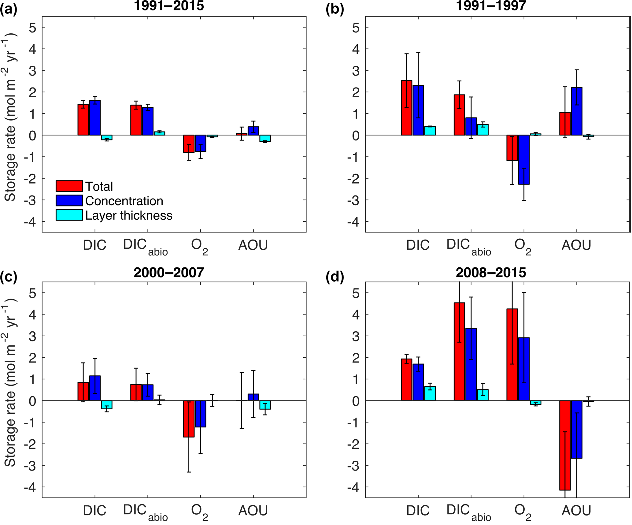
https://www.biogeosciences.net/15/51/2018/bg-15-51-2018-f10

Figure 10Decomposition of the total storage rates (red bars) into the concentration-driven storage rate (blue bars) and the layer-thickness-driven storage rate (cyan bars) for DIC, DIC_abio, O₂ and AOU from (a) 1991–2015, (b) 1991–1997, (c) 2000–2007 and (d) 2008–2015. The error bars represent the error of the linear regression model.

Download

On shorter timescales (Fig. 10b and c) all variables show large variations in the storage rates consistent with the already discussed changes in hydrography. In contrast to the findings of Tanhua and Keeling (2012), DIC and DIC_abio storage rates are positive over all time periods. This might be partly due to the increased data coverage in our study. Over the entire time period, DIC_abio underestimates C_ant by about 25 %. However, if the time period is too short, DIC_abio becomes much more variable because it includes solubility effects. For example, from 2000–2007 the DIC_abio underestimates the C_ant storage rate by 40 % (compare Figs. 9c and 10c), while from 2008–2015 the DIC_abio overestimates the C_ant storage rate by 20 % (compare Figs. 9d and 10d).

Similar to the C_ant storage rates, both periods before and after 1997 show a loss in O₂ despite stronger convection in the early 1990s. At the same time, the small increase in AOU does not reflect the constant inventory rate in DIC_nat before 1997, nor does the constant AOU storage rate reflect the loss in DIC_nat after 1997. Again, this is attributed to the fact that cLSW was mostly formed before 1991 (Yashayaev et al., 2007 a). The mean O₂ saturation degree over the entire water column was 89 % in the period from 1991 to 1997, which resulted in a high O₂ inventory of 750 ± 4 mol m⁻² indicative of the recent ventilation. After 1997, no re-ventilation took place and the mean O₂ saturation dropped 2 %, while the inventory decreased to 732 ± 4 mol m⁻². From 2008 to 2015, the O₂ saturation values increased to 89 % again due to the strong inventory increase of 4.3 ± 2.6 mol m⁻² yr⁻¹, which was mainly driven by the deep convection in 2015 (Fröb et al., 2016). Here, the strong loss in AOU matches the loss in DIC_nat as the water column is re-ventilated so that remineralized organic matter is replaced by a larger fraction of C_ant. In fact, the convection in 2015 was strong enough to restore the O₂ inventory levels so that the mean inventory from 2008 to 2015 was 749 ± 4 mol m⁻², the same level as the well-ventilated early 1990s.

7 Conclusions

The repeat observations within the Irminger Sea show significant changes in total, natural and anthropogenic CO₂ inventories from 1991 to 2015 with large interannual variability in the natural component. The eOMP method results and the decomposition of the inventory changes give valuable insight into the driving mechanisms to interpret the observed variability. Overall, changes in layer thickness of the main water masses appear most important for the DIC_nat inventory, while concentration change within these water masses is the key factor for C_ant. C_ant is typically more important for changes in total DIC inventories than DIC_nat. While the DIC inventory changes show a clear signal associated with the NAO, for C_ant the signal is less robust, especially before and after 1997, likely because the data used here do not cover the period before 1991 when the thick layer of cLSW was formed. From 1991 to 2015 the mean C_ant saturation over the entire water column increased from 52 to 67 %, increasing the C_ant inventory from 53 ± 3 to 117 ± 3 mol m⁻², mainly driven by the most recent convection in 2015. Despite the negative trend in O₂ inventory from 1991 to 2015, the convection in 2015 was strong enough to replenish O₂ levels at depth, leading to a mean saturation of 89 % and an O₂ inventory of 749 ± 4 mol m⁻², which was as high as in 1991. C_ant is sensitive to the time period considered, while DIC appears more robust to sampling and measurement bias. Therefore, for a comprehensive view on carbon cycle feedback mechanisms, not only C_ant but also natural and total DIC should be taken into account.

Data availability

The GLODAPv2 data are available under https://doi.org/10.3334/CDIAC/OTG.NDP093_GLODAPv2. The data from 29AH20120622 are available at https://cchdo.ucsd.edu/cruise/29AH20120622 and the 58GS20150410 data are currently being prepared for submission to CCHDO and PANGEA.

Appendix A: Salinity–alkalinity relationship

The application of the surface relationship between salinity, temperature and A_T by Lee et al. (2006) is tested for Irminger Sea cruise data in the entire water column. Further, the linear relationship between salinity and A_T by Nondal et al. (2009) is applied as well and compared to the Lee et al. (2006) relationship. For all cruise data between 1991 and 2015, the difference between measured and calculated A_T is presented in Fig. A1. Both relationships perform reasonably well. For the Lee et al. (2006) relationship there is no bias with depth, but measured A_T is slightly overestimated. The Nondal et al. (2009) relationship tends to overestimate the measured A_T in the surface ocean and underestimate measured A_T below 2000 m. Therefore the variance in the Nondal et al. (2009) relationship is much larger than for the Lee et al. (2006) relationship. Within this study, the Lee et al. (2006) relationship was chosen in order to calculate A_T.

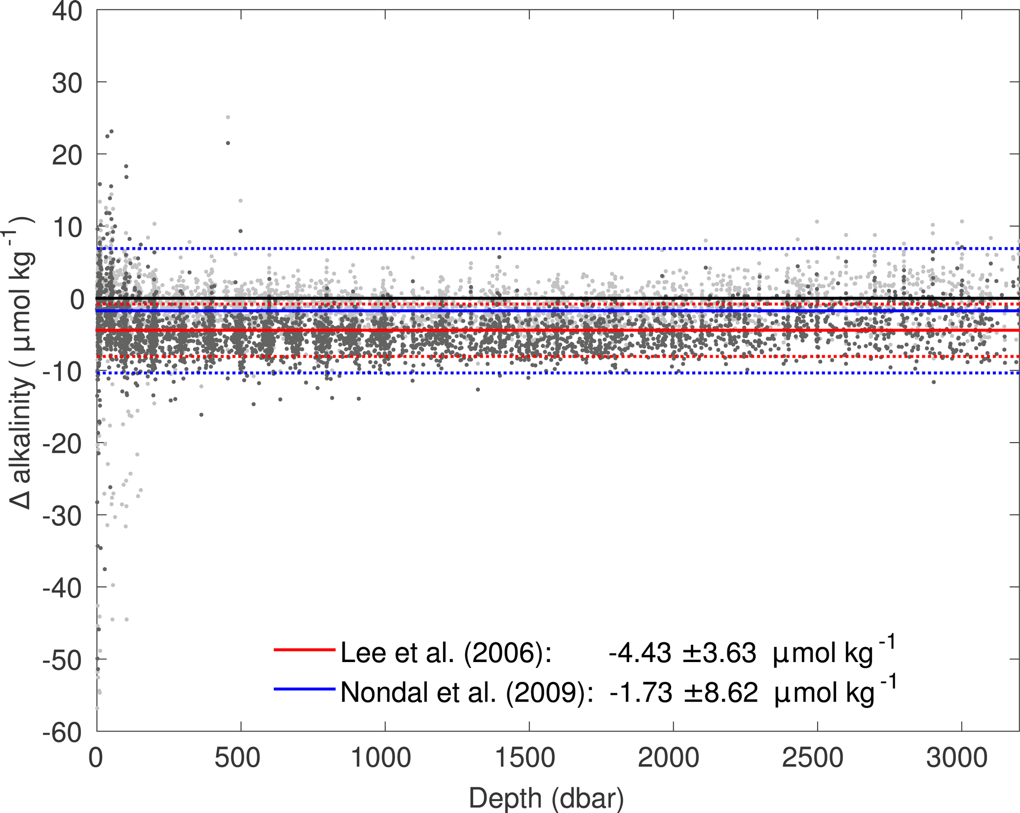
https://www.biogeosciences.net/15/51/2018/bg-15-51-2018-f11

Figure A1Difference between measured and calculated alkalinity for Irminger Sea cruise data. The dark grey dots use the salinity–alkalinity relationship following Lee et al. (2006) and the light grey dots use the relationship following Nondal et al. (2009). The solid lines represent the mean difference and dotted lines ± 1 SD (1 standard deviation).

Download

Further, the impact of the overestimated calculated A_T on C_ant, DIC_nat and DIC storage rates was tested. For that, 4.5 µmol kg⁻¹, which was the mean difference between measured and calculated A_T based on the Lee et al. (2006) relationship, was added to the calculated A_T for the three cruises on which only DIC was measured. The archetypal C_ant concentrations for all SWTs were less than 1 µmol kg⁻¹ smaller after the correction of A_T. No significant difference between the storage rates was evident.

Appendix B: Location SWT

As a result of the eOMP, the fraction of SWTs in each sampling point is estimated. Figure B1 shows this fraction for the 1991 (Fig. B1a) and the 2015 (Fig. B1b) data for IW, uLSW, cLSW, DSOW, ISOW and UW, which is the sum over ISW, NACW and SPMW. Overall, the position of the water masses is well represented through time.

https://www.biogeosciences.net/15/51/2018/bg-15-51-2018-f12

Figure B1Vertical cross section of fraction of water masses (IW, cLSW, uLSW, DSOW, ISOW and UW) in (a) 1991 and (b) 2015. Ratios below 0.1 are set to zero for clarity.

Download

Competing interests

The authors declare that they have no conflict of interest.

Acknowledgements

The authors would like to thank the two anonymous reviewers for their suggestions and comments. Friederike Fröb and Are Olsen appreciate funding from the SNACS project (229752), which is part of the KLIMAFORSK programme of the Norwegian Research Council. Emil Jeansson and Siv K. Lauvset received funding from the NRC project VENTILATE (229791). Fiz F. Pérez and Maribel I. García-Ibáñez were supported by the Spanish Ministry of Economy and Competitiveness through the BOCATS (CTM2013-41048-P) project co-funded by the Fondo Europeo de Desarrollo Regional 2007–2012 (FEDER). This is a contribution to the BIGCHANGE project of the Bjerknes Centre for Climate Research.

Edited by: Katja Fennel
Reviewed by: two anonymous referees

References

Álvarez, M., Pérez, F. F., Shoosmith, D. R., and Bryden, H. L.: Unaccounted role of Mediterranean Water in the drawdown of anthropogenic carbon, J. Geophys. Res.-Oceans, 110, C09S03, https://doi.org/10.1029/2004JC002633, 2005. a

Álvarez-Salgado, X. A., Nieto-Cid, M., Álvarez, M., Pérez, F. F., Morin, P., and Mercier, H.: New insights on the mineralization of dissolved organic matter in central, intermediate, and deep water masses of the northeast North Atlantic, Limnol. Oceanogr., 58, 681–696, https://doi.org/10.4319/lo.2013.58.2.0681, 2013. a, b

Amante, C. and Eakins, B.: ETOPO1 1 Arc-Minute Global Relief Model: Procedures, Data Sources and Analysis, NOAA Technical Memorandum NESDIS NGDC-24, National Geophysical Data Center, NOAA, Boulder, Colorado, USA, https://doi.org/10.7289/V5C8276M, 2009. a

Arora, V. K., Boer, G. J., Friedlingstein, P., Eby, M., Jones, C. D., Christian, J. R., Bonan, G., Bopp, L., Brovkin, V., Cadule, P., Hajima, T., Ilyina, T., Lindsay, K., Tjiputra, J. F., and Wu, T.: Carbon-Concentration and Carbon-Climate Feedbacks in CMIP5 Earth System Models, J. Climate, 26, 5289–5314, https://doi.org/10.1175/JCLI-D-12-00494.1, 2013. a

Bacon, S., Gould, W., and Jia, Y.: Open-ocean convection in the Irminger Sea, Geophys. Res. Lett., 30, 1246, https://doi.org/10.1029/2002GL016271, 2003. a

Castro, C., Pérez, F., Holley, S., and Ríos, A.: Chemical characterisation and modelling of water masses in the Northeast Atlantic, Prog. Oceanogr., 41, 249–279, https://doi.org/10.1016/S0079-6611(98)00021-4, 1998. a

Curry, R., McCartney, M., and Joyce, T.: Oceanic transport of subpolar climate signals to mid-depth subtropical waters, Nature, 391, 575–577, https://doi.org/10.1038/35356, 1998. a

de Jong, M. F. and de Steur, L.: Strong winter cooling over the Irminger Sea in winter 2014–2015, exceptional deep convection, and the emergence of anomalously low SST, Geophys. Res. Lett., 45, 7106–7113, https://doi.org/10.1002/2016GL069596, 2016. a, b

de Jong, M. F., van Aken, H. M., Våge, K., and Pickart, R. S.: Convective mixing in the central Irminger Sea: 2002–2010, Deep-Sea Res. Pt. I, 63, 36–51, https://doi.org/10.1016/j.dsr.2012.01.003, 2012. a, b

Dickson, A., Sabine, C., and Christian, J. E.: Guide to Best Practices for Ocean CO₂ Measurements, PICES Special Publication 3, North Pacific Marine Science Organization, Sidney, British Columbia, 191 pp., 2007. a

Dickson, R. and Brown, J.: The Production of North-Atlantic Deep-Water – Sources, Rates and Pathways, J. Geophys. Res.-Oceans, 99, 12319–12341, https://doi.org/10.1029/94JC00530, 1994. a

Friedlingstein, P., Cox, P., Betts, R., Bopp, L., Von Bloh, W., Brovkin, V., Cadule, P., Doney, S., Eby, M., Fung, I., Bala, G., John, J., Jones, C., Joos, F., Kato, T., Kawamiya, M., Knorr, W., Lindsay, K., Matthews, H. D., Raddatz, T., Rayner, P., Reick, C., Roeckner, E., Schnitzler, K. G., Schnur, R., Strassmann, K., Weaver, A. J., Yoshikawa, C., and Zeng, N.: Climate-carbon cycle feedback analysis: Results from the C⁴MIP model intercomparison, J. Climate, 19, 3337–3353, https://doi.org/10.1175/JCLI3800.1, 2006. a

Fröb, F., Olsen, A., Våge, K., Moore, K., Yashayaev, I., Jeansson, E., and Rajasakaren, B.: Irminger Sea deep convection injects oxygen and anthropogenic carbon to the ocean interior, Nat. Commun., 7, 13244, https://doi.org/10.1038/ncomms13244, 2016. a, b, c, d, e, f, g, h, i

García-Ibáñez, M. I., Pardo, P. C., Carracedo, L. I., Mercier, H., Lherminier, P., Ríos, A. F., and Pérez, F. F.: Structure, transports and transformations of the water masses in the Atlantic Subpolar Gyre, Prog. Oceanogr., 135, 18–36, https://doi.org/10.1016/j.pocean.2015.03.009, 2015. a, b, c, d, e, f

García-Ibáñez, M. I., Zunino, P., Fröb, F., Carracedo, L. I., Ríos, A. F., Mercier, H., Olsen, A., and Pérez, F. F.: Ocean acidification in the subpolar North Atlantic: rates and mechanisms controlling pH changes, Biogeosciences, 13, 3701–3715, https://doi.org/10.5194/bg-13-3701-2016, 2016. a, b

Gruber, N., Sarmiento, J., and Stocker, T.: An improved method for detecting anthropogenic CO₂ in the oceans, Global Biogeochem. Cy., 10, 809–837, https://doi.org/10.1029/96GB01608, 1996. a

Häkkinen, S. and Rhines, P.: Decline of subpolar North Atlantic circulation during the 1990s, Science, 304, 555–559, https://doi.org/10.1126/science.1094917, 2004. a

Hansen, B. and Østerhus, S.: North Atlantic-Nordic Seas exchanges, Prog. Oceanogr., 45, 109–208, https://doi.org/10.1016/S0079-6611(99)00052-X, 2000. a

Hátún, H., Sandø, A., Drange, H., Hansen, B., and Valdimarsson, H.: Influence of the Atlantic subpolar gyre on the thermohaline circulation, Science, 309, 1841–1844, https://doi.org/10.1126/science.1114777, 2005. a

Hood, E. M., Sabine, C. L., and Sloyan, B. M. (Eds.): The GO-SHIP Repeat Hydrography Manual: A Collection of Expert Reports and Guidelines, IOCCP Report Number 14, ICPO Publication Series Number 134, available at http://www.go-ship.org/HydroMan.html (last access: 5 October 2016), 2010. a

Hurrell, J. W. and Deser, C.: North Atlantic climate variability: The role of the North Atlantic Oscillation, J. Mar. Syst., 78, 28–41, 2009. a, b

Jeansson, E., Jutterström, S., Rudels, B., Anderson, L. G., Olsson, K. A., Jones, E. P., Smethie Jr., W. M., and Swift, J. H.: Sources to the East Greenland Current and its contribution to the Denmark Strait Overflow, Prog. Oceanogr., 78, 12–28, https://doi.org/10.1016/j.pocean.2007.08.031, 2008. a

Johnson, K., Key, R., Millero, F., Sabine, C., Wallace, D., Winn, C., Arlen, L., Erickson, K., Friis, K., Galanter, M., Goen, J., Rotter, R., Thomas, C., Wilke, R., Takahashi, T., and Sutherland, S.: Carbon Dioxide, Hydrographic, and Chemical Data Obtained During the R/V Knorr Cruises in the North Atlantic Ocean on WOCE Sections AR24 (November 2–December 5, 1996) and A24, A20, and A22 (May 30–September 3, 1997), Carbon Dioxide Information Analysis Center, Oak Ridge National Laboratory, US Department of Energy, Oak Ridge, Tennessee, 2003. a

Karstensen, J. and Tomczak, M.: Age determination of mixed water masses using CFC and oxygen data, J. Geophys. Res.-Oceans, 103, 18599–18609, https://doi.org/10.1029/98JC00889, 1998. a

Key, R., Kozyr, A., Sabine, C., Lee, K., Wanninkhof, R., Bullister, J., Feely, R., Millero, F., Mordy, C., and Peng, T.: A global ocean carbon climatology: Results from Global Data Analysis Project (GLODAP), Global Biogeochem. Cy., 18, GB4031, https://doi.org/10.1029/2004GB002247, 2004. a

Key, R. M., Tanhua, T., Olsen, A., Hoppema, M., Jutterström, S., Schirnick, C., van Heuven, S., Kozyr, A., Lin, X., Velo, A., Wallace, D. W. R., and Mintrop, L.: The CARINA data synthesis project: introduction and overview, Earth Syst. Sci. Data, 2, 105–121, https://doi.org/10.5194/essd-2-105-2010, 2010. a

Key, R. M., Olsen, A., van Heuven, S., Lauvset, S. K., Velo, A., Lin, X., Schirnick, C., Kozyr, A., Tanhua, T., Hoppema, M., Jutterström, S., Steinfeldt, R., Jeansson, E., Ishii, M., Pérez, F. F., and Suzuki, T.: Global Ocean Data Analysis Project, version 2 (GLODAPv2), ORNL/CDIAC-162, NDP-093, Carbon Dioxide Information Analysis Center, Oak Ridge National Laboratory, Oak Ridge, Tennessee, USA, 2015. a

Körtzinger, A., Rhein, M., and Mintrop, L.: Anthropogenic CO₂ and CFCs in the North Atlantic Ocean – A comparison of man-made tracers, Geophys. Res. Lett., 26, 2065–2068, https://doi.org/10.1029/1999GL900432, 1999. a

Landschützer, P., Gruber, N., Haumann, F. A., Rödenbeck, C., Bakker, D. C. E., van Heuven, S., Hoppema, M., Metzl, N., Sweeney, C., Takahashi, T., Tilbrook, B., and Wanninkhof, R.: The reinvigoration of the Southern Ocean carbon sink, Science, 349, 1221–1224, https://doi.org/10.1126/science.aab2620, 2015. a

Lavender, K., Owens, W., and Davis, R.: The mid-depth circulation of the subpolar North Atlantic Ocean as measured by subsurface floats, Deep-Sea Res. Pt. I, 52, 767–785, https://doi.org/10.1016/j.dsr.2004.12.007, 2005. a

Lazier, J., Hendry, R., Clarke, A., Yashayaev, I., and Rhines, P.: Convection and restratification in the Labrador Sea, 1990–2000, Deep-Sea Res. Pt. I, 49, 1819–1835, https://doi.org/10.1016/S0967-0637(02)00064-X, 2002. a, b

Lee, K., Tong, L. T., Millero, F. J., Sabine, C. L., Dickson, A. G., Goyet, C., Park, G.-H., Wanninkhof, R., Feely, R. A., and Key, R. M.: Global relationships of total alkalinity with salinity and temperature in surface waters of the world's oceans, Geophys. Res. Lett., 33, L19605, https://doi.org/10.1029/2006GL027207, 2006. a, b, c, d, e, f, g, h

Le Quéré, C., Rödenbeck, C., Buitenhuis, E. T., Conway, T. J., Langenfelds, R., Gomez, A., Labuschagne, C., Ramonet, M., Nakazawa, T., Metzl, N., Gillett, N., and Heimann, M.: Saturation of the Southern Ocean CO₂ Sink Due to Recent Climate Change, Science, 316, 1735–1738, https://doi.org/10.1126/science.1136188, 2007. a

Le Quéré, C., Andrew, R. M., Canadell, J. G., Sitch, S., Korsbakken, J. I., Peters, G. P., Manning, A. C., Boden, T. A., Tans, P. P., Houghton, R. A., Keeling, R. F., Alin, S., Andrews, O. D., Anthoni, P., Barbero, L., Bopp, L., Chevallier, F., Chini, L. P., Ciais, P., Currie, K., Delire, C., Doney, S. C., Friedlingstein, P., Gkritzalis, T., Harris, I., Hauck, J., Haverd, V., Hoppema, M., Klein Goldewijk, K., Jain, A. K., Kato, E., Körtzinger, A., Landschützer, P., Lefèvre, N., Lenton, A., Lienert, S., Lombardozzi, D., Melton, J. R., Metzl, N., Millero, F., Monteiro, P. M. S., Munro, D. R., Nabel, J. E. M. S., Nakaoka, S.-I., O'Brien, K., Olsen, A., Omar, A. M., Ono, T., Pierrot, D., Poulter, B., Rödenbeck, C., Salisbury, J., Schuster, U., Schwinger, J., Séférian, R., Skjelvan, I., Stocker, B. D., Sutton, A. J., Takahashi, T., Tian, H., Tilbrook, B., van der Laan-Luijkx, I. T., van der Werf, G. R., Viovy, N., Walker, A. P., Wiltshire, A. J., and Zaehle, S.: Global Carbon Budget 2016, Earth Syst. Sci. Data, 8, 605–649, https://doi.org/10.5194/essd-8-605-2016, 2016. a

Lherminier, P., Mercier, H., Huck, T., Gourcuff, C., Pérez, F. F., Morin, P., Sarafanov, A., and Falina, A.: The Atlantic Meridional Overturning Circulation and the subpolar gyre observed at the A25-OVIDE section in June 2002 and 2004, Deep-Sea Res. Pt. I, 57, 1374–1391, https://doi.org/10.1016/j.dsr.2010.07.009, 2010. a, b, c

Lueker, T. J., Dickson, A. G., and Keeling, C. D.: Ocean pCO₂ calculated from dissolved inorganic carbon, alkalinity, and equations for K₁ and K₂: validation based on laboratory measurements of CO₂ in gas and seawater at equilibrium, Mar. Chem., 70, 105–119, https://doi.org/10.1016/S0304-4203(00)00022-0, 2000. a

Marshall, J. and Schott, F.: Open-ocean convection: Observations, theory, and models, Rev. Geophys., 37, 1–64, https://doi.org/10.1029/98RG02739, 1999. a

Maze, G., Mercier, H., Thierry, V., Memery, L., Morin, P., and Pérez, F. F.: Mass, nutrient and oxygen budgets for the northeastern Atlantic Ocean, Biogeosciences, 9, 4099–4113, https://doi.org/10.5194/bg-9-4099-2012, 2012. a

McCartney, M.: Recirculating components to the deep boundary current of the northern North Atlantic, Prog. Oceanogr., 29, 283–383, https://doi.org/10.1016/0079-6611(92)90006-L, 1992. a

Meincke, J. and Becker, G.: Woce-Nord 1991, Nordsee 1991, Meteor-Berichte No. 93-1, 1993. a

Mercier, H., Lherminier, P., Sarafanov, A., Gaillard, F., Daniault, N., Desbruyères, D., Falina, A., Ferron, B., Gourcuff, C., Huck, T., and Thierry, V.: Variability of the meridional overturning circulation at the Greenland-Portugal OVIDE section from 1993 to 2010, Prog. Oceanogr., 132, 250–261, https://doi.org/10.1016/j.pocean.2013.11.001, 2015. a, b

Nondal, G., Bellerby, R. G. J., Olsen, A., Johannessen, T., and Olafsson, J.: Optimal evaluation of the surface ocean CO₂ system in the northern North Atlantic using data from voluntary observing ships, Limnol. Oceanogr., 7, 109–118, https://doi.org/10.4319/lom.2009.7.109, 2009. a, b, c, d

Olsen, A., Key, R. M., van Heuven, S., Lauvset, S. K., Velo, A., Lin, X., Schirnick, C., Kozyr, A., Tanhua, T., Hoppema, M., Jutterström, S., Steinfeldt, R., Jeansson, E., Ishii, M., Pérez, F. F., and Suzuki, T.: The Global Ocean Data Analysis Project version 2 (GLODAPv2) – an internally consistent data product for the world ocean, Earth Syst. Sci. Data, 8, 297–323, https://doi.org/10.5194/essd-8-297-2016, 2016. a, b, c

Palter, J. B., Caron, C.-A., Law, K. L., Willis, J. K., Trossman, D. S., Yashayaev, I. M., and Gilbert, D.: Variability of the directly observed, middepth subpolar North Atlantic circulation, Geophys. Res. Lett., 43, 2700–2708, doi10.1002/2015GL067235, 2016. a

Pérez, F. F., Vázquez-Rodríguez, M., Louarn, E., Padín, X. A., Mercier, H., and Ríos, A. F.: Temporal variability of the anthropogenic CO₂ storage in the Irminger Sea, Biogeosciences, 5, 1669–1679, https://doi.org/10.5194/bg-5-1669-2008, 2008. a, b, c, d, e, f, g

Pérez, F. F., Vázquez-Rodríguez, M., Mercier, H., Velo, A., Lherminier, P., and Ríos, A. F.: Trends of anthropogenic CO₂ storage in North Atlantic water masses, Biogeosciences, 7, 1789–1807, https://doi.org/10.5194/bg-7-1789-2010, 2010. a

Pérez, F. F., Mercier, H., Vázquez-Rodríguez, M., Lherminier, P., Velo, A., Pardo, P. C., Roson, G., and Ríos, A. F.: Atlantic Ocean CO₂ uptake reduced by weakening of the meridional overturning circulation, Nat. Geosci., 6, 146–152, https://doi.org/10.1038/NGEO1680, 2013. a

Pickart, R., Spall, M., Ribergaard, M., Moore, G., and Milliff, R.: Deep convection in the Irminger Sea forced by the Greenland tip jet, Nature, 424, 152–156, https://doi.org/10.1038/nature01729, 2003a. a, b

Pickart, R., Straneo, F., and Moore, G.: Is Labrador Sea Water formed in the Irminger basin?, Deep-Sea Res. Pt. I, 50, 23–52, https://doi.org/10.1016/S0967-0637(02)00134-6, 2003b. a, b, c

Poole, R. and Tomczak, M.: Optimum multiparameter analysis of the water mass structure in the Atlantic Ocean thermocline, Deep-Sea Research Pt. I, 46, 1895–1921, https://doi.org/10.1016/S0967-0637(99)00025-4, 1999. a

Ríos, A. F., Pérez, F. F., García-Ibáñez, M. I., Fajar, N. M., Lherminier, P., Branellec, P., Gilcoto, M., Rosón, G., Alonso-Pérez, F., de la Paz, M., Castaño-Carrera, M., Galindo, M., and Velo, A.: Carbon Dioxide, Hydrographic, and Chemical Data Obtained During the R/V Sarmiento de Gamboa Cruise in the North Atlantic Ocean on CLIVAR Repeat Hydrography Section OVIDE-2012 (June 22–July 20, 2012). Carbon Dioxide Information Analysis Center, Oak Ridge National Laboratory, US Department of Energy, Oak Ridge, Tennessee, 2015. a

Sabine, C. and Tanhua, T.: Estimation of anthropogenic CO₂ inventories in the ocean, Annu. Rev. Mar. Sci., 2, 175–198, https://doi.org/10.1146/annurev-marine-120308-080947, 2010. a

Sabine, C., Feely, R., Gruber, N., Key, R., Lee, K., Bullister, J., Wanninkhof, R., Wong, C., Wallace, D., Tilbrook, B., Millero, F., Peng, T., Kozyr, A., Ono, T., and Ríos, A.: The oceanic sink for anthropogenic CO₂, Science, 305, 367–371, https://doi.org/10.1126/science.1097403, 2004. a, b

Sarafanov, A., Falina, A., Sokov, A., and Demidov, A.: Intense warming and salinification of intermediate waters of southern origin in the eastern subpolar North Atlantic in the 1990s to mid-2000s, J. Geophys. Res.-Oceans, 113, C12022, https://doi.org/10.1029/2008JC004975, 2008. a

Sarmiento, J. and Gruber, N.: Sinks for anthropogenic carbon, Physics Today, 55, 30–36, https://doi.org/10.1063/1.1510279, 2002. a

Schwinger, J., Tjiputra, J. F., Heinze, C., Bopp, L., Christian, J. R., Gehlen, M., Ilyina, T., Jones, C. D., Salas-Melia, D., Segschneider, J., Seferian, R., and Totterdell, I.: Nonlinearity of Ocean Carbon Cycle Feedbacks in CMIP5 Earth System Models, J. Climate, 27, 3869–3888, https://doi.org/10.1175/JCLI-D-13-00452.1, 2014. a, b

Steinfeldt, R., Rhein, M., Bullister, J. L., and Tanhua, T.: Inventory changes in anthropogenic carbon from 1997–2003 in the Atlantic Ocean between 20^∘ S and 65^∘ N, Global Biogeochem. Cy., 23, GB3010, https://doi.org/10.1029/2008GB003311, 2009. a

Stendardo, I. and Gruber, N.: Oxygen trends over five decades in the North Atlantic, J. Geophys. Res.-Oceans, 117, C11004, https://doi.org/10.1029/2012JC007909, 2012. a

Stoll, M., van Aken, H., de Baar, H., and de Boer, C.: Meridional carbon dioxide transport in the northern North Atlantic, Mar. Chem., 55, 205–216, https://doi.org/10.1016/S0304-4203(96)00057-6, 1996. a

Straneo, F., Pickart, R. S., and Lavender, K.: Spreading of Labrador sea water: an advective-diffusive study based on Lagrangian data, Deep-Sea Res. Pt. I, 50, 701–719, https://doi.org/10.1016/S0967-0637(03)00057-8, 2003. a

Tanhua, T. and Keeling, R. F.: Changes in column inventories of carbon and oxygen in the Atlantic Ocean, Biogeosciences, 9, 4819–4833, https://doi.org/10.5194/bg-9-4819-2012, 2012. a, b, c, d, e, f, g

Tanhua, T., Olsson, K. A., and Jeansson, E.: Formation of Denmark Strait overflow water and its hydro-chemical composition, J. Mar. Syst., 57, 264–288, https://doi.org/10.1016/j.jmarsys.2005.05.003, 2005. a, b, c, d, e, f

Thomas, H. and Ittekkot, V.: Determination of anthropogenic CO₂ in the North Atlantic Ocean using water mass ages and CO₂ equilibrium chemistry, J. Marine Syst., 27, 325–336, https://doi.org/10.1016/S0924-7963(00)00077-4, 2001. a

Tomczak, M. and Large, D. G. B.: Optimum Multimparameter Analysis of Mixing in the Thermocline of the Eastern Indian-Ocean, J. Geophys. Res.-Oceans, 94, 16141–16149, https://doi.org/10.1029/JC094iC11p16141, 1989. a

Touratier, F. and Goyet, C.: Decadal evolution of anthropogenic CO₂ in the northwestern Mediterranean Sea from the mid-1990s to the mid-2000s, Dee-Sea Res. Pt. I, 56, 1708–1716, https://doi.org/10.1016/j.dsr.2009.05.015, 2009. a

van Aken, H.: The hydrography of the mid-latitude Northeast Atlantic Ocean II: The intermediate water masses, Deep-Sea Res. Pt. I, 47, 789–824, https://doi.org/10.1016/S0967-0637(99)00112-0, 2000. a

van Heuven, S., Zemmelink, H., Bakker, K., van Aken, H., and Veth, C.: Carbon Dioxide, Hydrographic, and Chemical Data Obtained During the R/V Pelagia Repeat Hydrography Cruise in the Atlantic Ocean: CLIVAR CO₂ Section AR07E2005 (September 7–October 5, 2005), Carbon Dioxide Information Analysis Center, Oak Ridge National Laboratory, US Department of Energy, Oak Ridge, Tennessee, 2012. a

van Heuven, S., Brummer, G.-J., van Ooijen, J., and van Aken, H.: Carbon Dioxide, Hydrographic, and Chemical Data Obtained During the R/V Pelagia Repeat Hydrography Cruise in the Atlantic Ocean: CLIVAR CO₂ Section AR07E2007 (August 30–September 27, 2007), Carbon Dioxide Information Analysis Center, Oak Ridge National Laboratory, US Department of Energy, Oak Ridge, Tennessee, 2013. a

Vázquez-Rodríguez, M., Touratier, F., Lo Monaco, C., Waugh, D. W., Padin, X. A., Bellerby, R. G. J., Goyet, C., Metzl, N., Ríos, A. F., and Pérez, F. F.: Anthropogenic carbon distributions in the Atlantic Ocean: data-based estimates from the Arctic to the Antarctic, Biogeosciences, 6, 439–451, https://doi.org/10.5194/bg-6-439-2009, 2009. a, b, c

Vázquez-Rodríguez, M., Padín, X. A., Pardo, P. C., Ríos, A. F., and Pérez, F. F.: The subsurface layer reference to calculate preformed alkalinity and air-sea CO₂ disequilibrium in the Atlantic Ocean, J. Mar. Syst., 94, 52–63, https://doi.org/10.1016/j.jmarsys.2011.10.008, 2012. a, b

Våge, K., Pickart, R. S., Moore, G. W. K., and Ribergaard, M. H.: Winter mixed layer development in the central Irminger Sea: The effect of strong, intermittent wind events, J. Phys. Oceanogr., 38, 541–565, https://doi.org/10.1175/2007JPO3678.1, 2008. a, b

Våge, K., Pickart, R. S., Sarafanov, A., Knutsen, O., Mercier, H., Lherminier, P., van Aken, H. M., Meincke, J., Quadfasel, D., and Bacon, S.: The Irminger Gyre: Circulation, convection, and interannual variability, Deep-Sea Res. Pt. I, 58, 590–614, https://doi.org/10.1016/j.dsr.2011.03.001, 2011. a, b

Wakita, M., Watanabe, S., Murata, A., Tsurushima, N., and Honda, M.: Decadal change of dissolved inorganic carbon in the subarctic western North Pacific Ocean, Tellus B, 62, 1600–0889, https://doi.org/10.1111/j.1600-0889.2010.00476.x, 2010. a

Wanninkhof, R., Doney, S. C., Bullister, J. L., Levine, N. M., Warner, M., and Gruber, N.: Detecting anthropogenic CO₂ changes in the interior Atlantic Ocean between 1989 and 2005, J. Geophys. Res.-Oceans, 115, C11028, https://doi.org/10.1029/2010JC006251, 2010. a

Woosley, R. J., Millero, F. J., and Wanninkhof, R.: Rapid anthropogenic changes in CO₂ and pH in the Atlantic Ocean: 2003–2014, Global Biogeochem. Cy., 30, 70–90, https://doi.org/10.1002/2015GB005248, 2016. a

Yashayaev, I., Bersch, M., and van Aken, H. M.: Spreading of the Labrador Sea Water to the Irminger and Iceland basins, Geophys. Res. Lett., 34, l10602, https://doi.org/10.1029/2006GL028999, 2007a. a, b, c, d, e, f

Yashayaev, I., van Aken, H. M., Holliday, N. P., and Bersch, M.: Transformation of the Labrador Sea Water in the subpolar North Atlantic, Geophys. Res. Lett., 34, L22605, https://doi.org/10.1029/2007GL031812, 2007b. a, b, c

Zunino, P., Lherminier, P., Mercier, H., Padín, X. A., Ríos, A. F., and Pérez, F. F.: Dissolved inorganic carbon budgets in the eastern subpolar North Atlantic in the 2000s from in situ data, Geophys. Res. Lett., 42, 9853–9861, https://doi.org/10.1002/2015GL066243, 2015. a

Articles

Short summary

On long timescales, the inventory of total dissolved inorganic carbon in the ocean is mainly driven by the increase in anthropogenic CO₂ emitted to the atmosphere due to human activities. On short timescales, however, the anthropogenic signal can be masked by the variability in natural inorganic carbon, shown in this study based on Irminger Sea cruise data from 1991 to 2015. In order to estimate oceanic carbon budgets, we suggest jointly assessing natural, anthropogenic and total carbon.

Inorganic carbon and water masses in the Irminger Sea since 1991

4.1 Anthropogenic CO2 calculation

4.2 Extended optimum multiparameter analysis (eOMP)

4.3 Uncertainty analysis

5.1 SWT distribution

5.2 Archetypal concentration changes

5.3 DIC storage rate decomposition

4.1 Anthropogenic CO₂ calculation