2.1.1 Causes of δChl by advective processes

Mesoscale eddies may cause δChl as they laterally move waters (i.e., horizontally advect waters) including their Chl characteristics. This mechanism may lead to δChl if (i) a lateral Chl gradient is present that is sufficiently steep at the spatial scale of the eddy-induced advection (Gaube et al., 2014), and (ii) the time scale of advection matches the time scale of phytoplankton biomass changes (Abraham, 1998). The latter time scale is in the order of days to weeks, possibly months, with the lower boundary representing roughly the reactivity time scale of phytoplankton biomass governed largely by the growth rate of the phytoplankton, and the upper boundary the potential sustenance of phytoplankton biomass via recycling of nutrients within the mixed layer. In regard to the spatial scale of advection by eddies, we distinguish two effects, that we have labeled stirring and trapping.

Stirring (Chelton et al., 2011a; Gaube et al., 2014; McGillicuddy Jr., 2016; Siegel et al., 2008) refers to the local distortion of a large-scale Chl gradient due to the rotation of an eddy, as illustrated in Fig. 1a, left column. The turnover time scale associated with the rotation of eddies is in the order of days to a few weeks, matching the time scales of phytoplankton reactivity. The spatial scale of stirring is given by the spatial extent of an eddy and is somewhat larger than the eddy core, as defined based on the Okubo–Weiss parameter (Frenger et al., 2015), that is several tens to several hundreds of kilometers.

Next to stirring, eddies advect material properties due to their intrinsic lateral propagation (Fig. 1a, right column). We refer to the ability of eddies to transport fluid along their propagation pathway in their core as trapping (Flierl, 1981; Gaube et al., 2014; McGillicuddy Jr., 2016). The upper time scale of trapping is given by the typical lifespan of Southern Ocean mesoscale eddies, which is weeks to months (Frenger et al., 2015), it may thus match the longer time scale of phytoplankton biomass changes. Propagation speeds are low (an order of magnitude smaller than rotational speeds), which implies that the majority of eddies tends to die before they can propagate far. Thus, the fraction of very long-lived eddies that propagate over distances exceeding a few hundred kilometers is small (Frenger et al., 2015).

A necessary condition for trapping to happen is that the eddies' swirl velocity is larger than their propagation speed (Flierl, 1981), a condition generally met for mid- to high-latitude eddies (Chelton et al., 2011b). Indeed, observations of eddies carrying the signature of their origin in their cores support the trapping effect (Ansorge et al., 2010; Bernard et al., 2007; Lehahn et al., 2011), as does the modeling study by Early et al. (2011). Even though the trapping is never perfect (Beron-Vera et al., 2013; Haller, 2015), we expect eddies to be able to drag along some entrained waters for some time, hence displacing these waters for some distance as they propagate. This may be sufficient to displace waters from e.g., the south to the north of an ACC front along an intense Chl gradient, leading to δChl through (permeable) trapping.

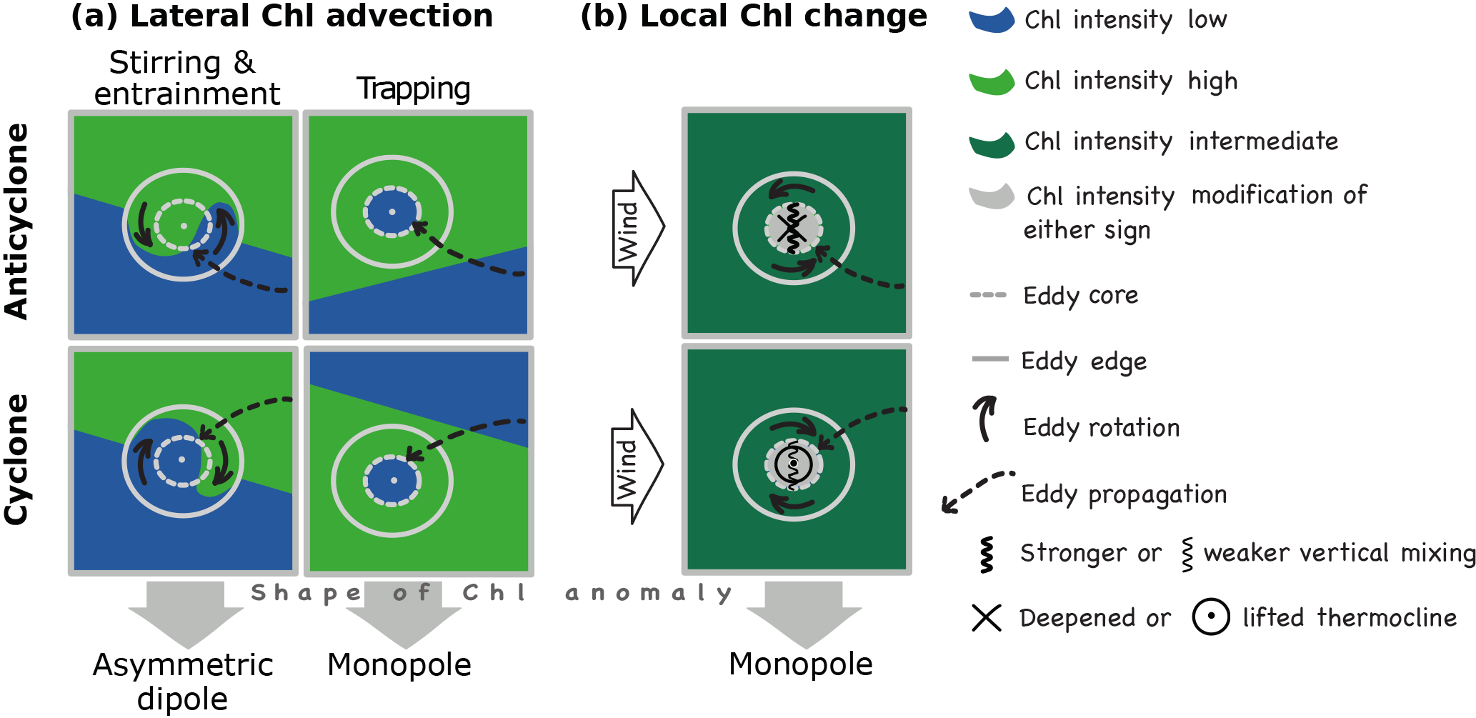
Figure 1Schematic illustrating the mechanisms of how eddies may impact chlorophyll (Chl), for anticyclones (top row) and cyclones (bottom row), for the southern hemisphere; (a) shows the effects of advection (lateral displacements) of Chl due to the eddies' rotational speed (stirring, left column) and lateral propagation (trapping, right column); trapping and stirring can cause δChl of either sign, depending on environmental Chl gradients; (b) shows multiple potential effects eddies may have on Chl by affecting biogeochemical processes. The local shape of δChl is anticipated to look different depending on the mechanism active, i.e., a monopole δChl is expected for all eddy-effects except for stirring where an asymmetric dipole is excepted (figure inspired by Siegel et al., 2011, Fig. 1).

Download

2.1.2 Causes of δChl by local biogeochemical processes

Mesoscale eddies affect the biogeochemical and physical properties that control the local rates of growth and loss of phytoplankton (biogeochemical rates) in their interior through many mechanisms. These include the stimulation of phytoplankton growth through enhanced nutrient concentrations or increased average light levels, or the modification of predator–prey encounter rates, affecting the mortality of phytoplankton (Fig. 1b). Even though these effects have been analyzed and discussed for decades (McGillicuddy Jr., 2016), their overall impact on productivity continues to be an issue of debate. The canonical lifelong vertical pumping of nutrients by thermocline lifted cyclones (Falkowski et al., 1991) has been challenged (Gaube et al., 2014; Oschlies, 2002), and multiple other mechanisms have been proposed on how eddies may affect phytoplankton biogeochemical rates. These include a modification of vertical mixing through changes in stratification (wiggly lines in Fig. 1b) and eddy current-wind interactions causing thermocline displacements (eddy swirl currents and winds are indicated as black and thick white arrows in Fig. 1b), resulting in modifications of nutrient supply and light availability to phytoplankton (Boyd et al., 2012; Dufois et al., 2016; Lehahn et al., 2011; Llido, 2005; Mahadevan et al., 2008, 2012; McGillicuddy Jr. et al., 2007; Siegel et al., 2011; Xiu et al., 2011). The prevailing lack of temporally sufficiently highly resolved subsurface observations hampers a systematic large-scale observationally based assessment of the role of effects of mesoscale eddies on the local biogeochemical processes.

2.1.3 Assessing mechanisms causing δChl

We employ two sets of approaches to assess the mechanisms causing δChl. In the first we diagnose whether the environmental conditions are supporting a major contribution of a particular set of mechanisms. Namely, we assess if lateral Chl gradients sufficiently support advective effects of eddies to explain δChl (see Sect. 2.3 for technical detail).

In the second set we diagnose the shape of δChl associated with eddies as this spatial signature tends to differ between the two major sets of processes, i.e., the advective process stirring and biogeochemical rates Siegel et al. (2011). Eddies that stir are anticipated to have a dipole shaped δChl (Fig. 1a, left column), as they distort the underlying gradient field, with the rotation of the eddy determining the orientation of the dipole. In contrast, most mechanisms associated with modifications of the biogeochemical rates cause a monopole shape, irrespective of polarity (Fig. 1b). This is a consequence of the mesoscale δChl tending to be caused by anomalies in nutrient supply or light exposure, which are altered inside eddies in a radially symmetric manner. The advective trapping mechanism tends to also cause a monopole shape of δChl (Fig. 1a, right column), but rate-based mechanisms can be distinguished from trapping for instance by their history (McGillicuddy Jr., 2016). Here we diagnose these as a residual: Rate-based mechanisms presumably play a role in regions and seasons where advective effects are insufficient to explain the observed eddy-induced δChl.

Some complexity is added to the interpretation of the spatial signature by the fact that the dipole shape arising from stirring tends to be asymmetric (Fig. 1a). Such an asymmetry was suggested by Chelton et al. (2011a) to arise from the westward propagation of eddies and the leading (mostly western) side of an eddy affecting upstream unperturbed waters, resulting in a larger anomaly at the leading compared to the trailing side of an eddy, with the latter stirring already perturbed waters. Also, the eddy may entrain some of the westward upstream waters into its core, labeled here lateral entrainment or permeable trapping (Frenger et al., 2015; Hausmann and Czaja, 2012). Indeed, averaged over an eddy's core, stirring will only cause a net anomaly if the dipole associated with stirring is asymmetric. It is not obvious how to quantify this effect. Independent of the dipole asymmetry, we will assess the potential maximum δChl induced by stirring (see Sect. 2.4 for technical detail). We note that advection by an ambient larger-scale flow does not affect the stirring mechanism. For instance, the eastward Antarctic circumpolar flow in the Southern Ocean makes eddies propagate eastward in an Eulerian sense, while still propagating westward in a Lagrangian sense relative to the ACC and ambient Chl.

3.1.1 Mean imprint

Averaged across the entire Southern Ocean and all seasons, we detect a significant, although small, mean imprint of mesoscale eddies on Chl (Fig. S1 in the Supplement) for both anticyclonic (warm-core, high SLA, and deepened thermocline) and cyclonic (cold-core, low SLA, and lifted thermocline) eddies. The overall mean δChl associated with anticyclones is −4  %, while that for cyclones is of even smaller magnitude, i.e., +1  %. Though small, both anomalies are actually statistically significant (p<0.05). However, the distributions around these means are very broad, with many anticyclones and cyclones having both positive or negative δChl, depending on the region and time of the year. The long tails of the distributions, corroborated by visual inspection of the individual δChl of eddies, suggest anomalies that are substantially larger than the mean. Thus, it appears that by averaging the signals in time and space, a substantial amount of information is lost. As a consequence, it is more insightful to disentangle the signals and to examine the regional and seasonal variation of δChl.

3.1.2 Spatial variability of imprint

The maps of the annual mean imprint of cyclonic and anticyclonic eddies on Chl clearly support the hypothesis of a strong regional cancellation effect (Fig. 2). First, the regional mean signal associated with eddies is indeed much larger than suggested by the mean δChl across the entire Southern Ocean. In fact, around a quarter of the analyzed grid cells have absolute δChl larger than 10 %, with the mean absolute δChl exceeding several tens of percent in a substantial number of grid cells (Fig. 2b, c). Second, the signals associated with mesoscale eddies of either polarity vary in sign across the different regions with regions of strong enhancements bordering regions with strong reductions (see also Fig. 1 in Gaube et al., 2014). In the broadest sense, the pattern is zonal in nature, reflecting the zonal nature of the climatological Chl distribution (Fig. 2a).

Figure 2Spatial distribution of chlorophyll anomalies (δChl) associated with eddies; (a) logarithm (base 10) of annual climatological Chl for reference, and mean δChl of (b) anticyclones and (c) cyclones; δChl is the average of anomalies of eddies lasting at least 3 weeks in $\mathrm{5}{}^{\circ }\times \mathrm{3}{}^{\circ }$ longitude–latitude grid boxes; white boxes indicate insufficient data (less than three data points) or anomalies insignificantly different from zero (t test, p=0.05); solid black lines mark the main branches of the ACC (the Subantarctic Front and Polar Front); the dashed black line denotes the −20 cm SSH contour and the solid gray line the northernmost extension of sea-ice cover.

Download

For anticyclones, δChl is clearly negative in subtropical waters, i.e., the waters north of the SSH $=-\mathrm{20}$ cm, and in the regions around the western boundary currents (Fig. 2b). These prevailing negative δChl are contrasted by mostly positive δChl along the ACC. Cyclones have a largely similar spatial pattern, but of opposite sign (Fig. 2c). That is, prevailing positive δChl in subtropical waters are mirrored by a band of negative, yet weaker anomalies along the ACC. South of the ACC, in Antarctic waters, the pattern of δChl is spotty for anticyclones as well as cyclones, with anticyclones and cyclones featuring average positive and negative δChl, respectively. In summary, SLA and δChl are largely negatively correlated in subtropical waters north of the ACC, and positively correlated along the ACC.

A few exceptions break the mostly zonal pattern for Chl (Ardyna et al., 2017), and also for δChl. An exceptional area of negative δChl for cyclones in the subtropical waters of the eastern Indian Ocean disrupts the zonal band of largely positive anomalies. Also, δChl in shelf areas often are distinct from open-ocean δChl. A clear signal emerges south of the Australian and west of the South American coasts, west of New Zealand, and more subtly, east of the Kerguelen Islands and the Drake Passage (see also Sokolov and Rintoul, 2007; d'Ovidio et al., 2015), where δChl tends to be positive for both anticyclones and cyclones.

3.1.3 Seasonality of imprint

The pronounced zonal bands of δChl for mesoscale anticyclones and cyclones persist over the year, but tend to migrate meridionally (Fig. 3a–d, middle and right columns), thereby following the pronounced seasonality of Chl (Fig. 3a–d, left column; Ardyna et al., 2017; Sallée et al., 2015; Thomalla et al., 2011). The seasonality of δChl is larger along the ACC and in Antarctic waters compared to subtropical waters. In the subtropical gyres, δChl of anticyclones and cyclones are negative and positive, respectively, i.e., SLA and δChl are negatively correlated all year round. Here, δChl shows a weak peak in austral summer when climatological Chl is lowest (Fig. 3c). In the ACC regions and in Antarctic waters, a striking feature is the seasonal change in the sign of δChl for both cyclones and anticyclones (Fig. 3b–d).

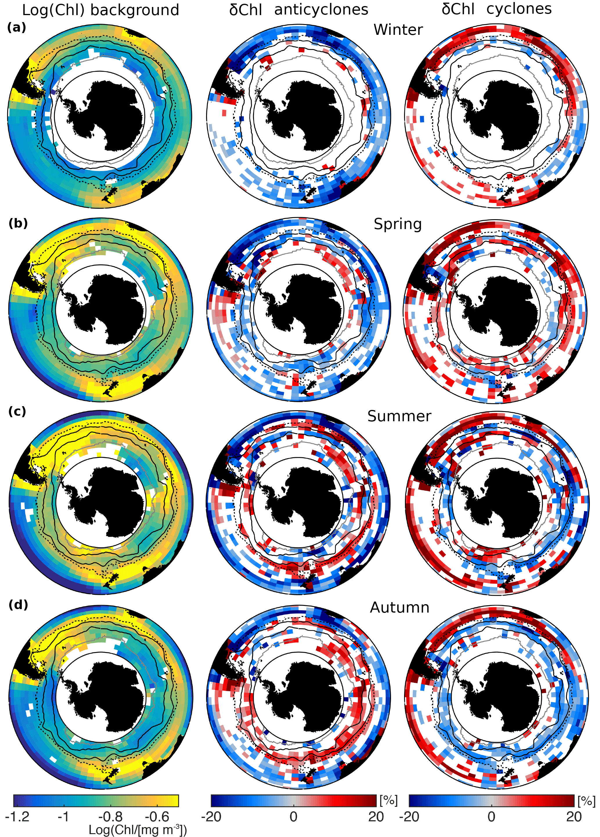
Figure 3Seasonality of chlorophyll anomalies (δChl) associated with eddies; austral (a) winter (JJA), (b) spring (SON), (c) summer (DJF), and (d) autumn (MAM) for anticyclones (middle) and cyclones (right); The logarithm (base 10) of seasonal climatological Chl is shown for reference (left). Otherwise the same as Fig. 2.

Download

This becomes even more evident when inspecting the zonally averaged Chl and δChl as a function of season and SSH, i.e., plotted in the form of a Hovmoeller diagram (Fig. 4). Along the ACC, anticyclones exhibit negative δChl in winter to spring concurrent with deep mixed layers, followed by positive δChl from summer to autumn (Fig. 4b). Cyclonic δChl shows an opposite pattern, featuring negative δChl from summer to autumn, with near to zero to positive δChl in winter to spring (Fig. 4c). This implies that SLA and δChl are positively correlated summer to autumn, followed by a negative correlation in winter to spring. The sign switch of the correlations shows a seasonal lag towards Antarctic waters, with positive correlations prevailing from autumn to winter, and negative correlations prevailing from spring to summer, resulting in the aforementioned apparent southward migration of the sign switch of the δChl over the course of the year.

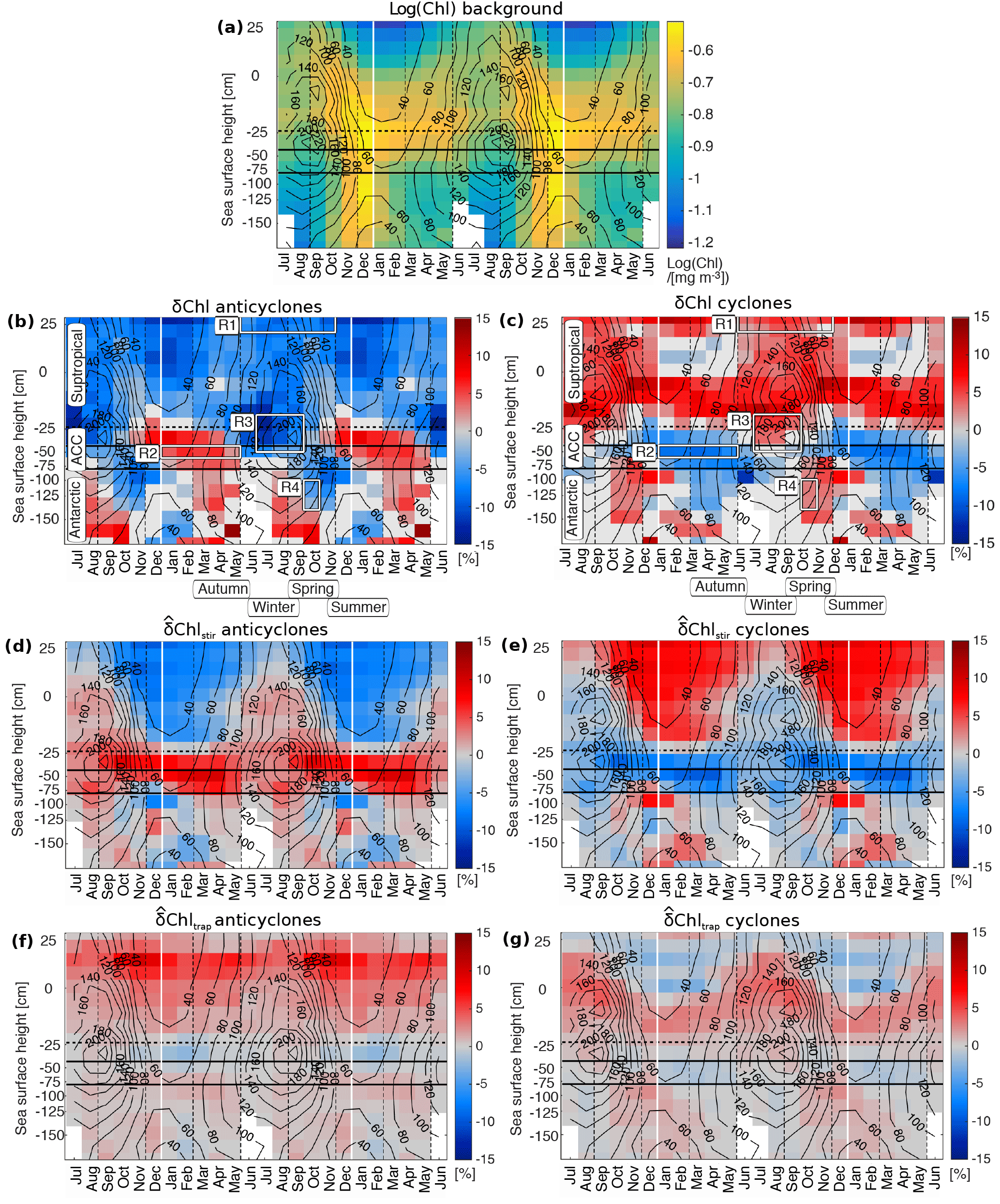
Figure 4Seasonality of chlorophyll anomalies (δChl) associated with eddies, and potential of eddies to cause δChl through lateral advection, i.e., $\widehat{\mathit{\delta }}{\mathrm{Chl}}_{\mathrm{stir}}$ for stirring and $\widehat{\mathit{\delta }}{\mathrm{Chl}}_{\mathrm{trap}}$ for trapping. (a) Base 10 logarithm of monthly climatological Chl for reference; (b, c) δChl related to anticyclones and cyclones, respectively; (d, e) advective potential (Sect. 2.3) due to stirring by anticyclones and cyclones, respectively; (f, g), advective potentials due to trapping by anticyclones and cyclones, respectively. In panels (a)–(c), Chl and δChl are the mean of all eddies lasting at least 3 weeks binned in monthly sea surface height (SSH) bins so that boxes roughly cover equal areas; in panels (b, c) white boxes indicate regions R1 to R4 used for composite Figs. 5 and 6. In all subpanels, values that are not significant (t test, p>0.05) are colored in light gray, insufficient data (less than three data points) in white; solid black lines mark the ACC (approximate positions of the Subantarctic Front and Polar Front); the horizontal dashed black line denotes the −20 cm SSH contour, the vertical dashed lines seasons; solid black contours show averaged mixed layer depths in meters; note that the seasonal cycle is shown repeatedly to highlight cyclic patterns.

Download

3.2.1 Advection

To assess the contribution of advective mechanisms to the observed δChl, we contrast it with the potential of eddies to cause δChl through Chl advection, that is with the potentials $\widehat{\mathit{\delta }}{\mathrm{Chl}}_{\mathrm{stir}}$ associated with stirring and $\widehat{\mathit{\delta }}{\mathrm{Chl}}_{\mathrm{trap}}$, associated with trapping (Fig. 4d–g, Method Sect. 2.3). The closer the observed δChl is to these parameters, the more important the respective processes would be in causing this signal.

In the northern domain, i.e., in subtropical waters, the sign of $\widehat{\mathit{\delta }}{\mathrm{Chl}}_{\mathrm{stir}}$ tends to agree with δChl throughout the year for both anticyclones and cyclones (Fig. 4b–e). So does the seasonal variation of the magnitude of $\widehat{\mathit{\delta }}{\mathrm{Chl}}_{\mathrm{stir}}$, with the largest magnitudes found from summer to autumn. Also the regional variations match, such as a weaker $\widehat{\mathit{\delta }}{\mathrm{Chl}}_{\mathrm{stir}}$ and δChl in the Pacific sector compared to the Atlantic and Indian Ocean sectors (Fig. 3, middle and right columns and Supplement Fig. S2, left column).

Furthermore, along the ACC and its northern flank, $\widehat{\mathit{\delta }}{\mathrm{Chl}}_{\mathrm{stir}}$ and δChl agree in sign, and are of the same order of magnitude from summer to autumn. Finally, along the southern ACC and in Antarctic waters, $\widehat{\mathit{\delta }}{\mathrm{Chl}}_{\mathrm{stir}}$ mirrors the seasonal sign switch of δChl, and the apparent seasonal southward migration of the zonal bands of δChl (Figs. 3 and 4b–e). Thus, it appears that stirring can already explain a good fraction of the observed δChl (i) in subtropical waters outside of those characterized by winter deep mixed layers, (ii) along the ACC and its northern flank from summer to autumn, and (iii) south of the ACC.

The reason underlying the strong potential of stirring is the presence of strong lateral gradients of Chl. For instance, averaged over mesoscale eddies in northern subtropical waters from winter to spring (Method Sect. 2.4), the absolute ambient gradient of Chl at scales of two eddy radii is 7 % for both anticyclones and cyclones, compared to the absolute maximum δChl of 10 % and 9 %, respectively (Fig. 5a, see numbers at the bottoms of left two panels). A similar correspondence is found along the ACC and its northern flank from summer to autumn (Fig. 6a), and in Antarctic waters during spring (Fig. 5b), supporting that stirring alone may largely explain the observed δChl (Fig. 6a; anticyclones: gradient of 9 % and maximum δChl of 5 %; cyclones: gradient of 9 % and maximum δChl of 11 %; and Fig. 5b; anticyclones: gradient of 5 % and maximum δChl of 6 %; cyclones: gradient of 5 % and maximum δChl of 5 %).

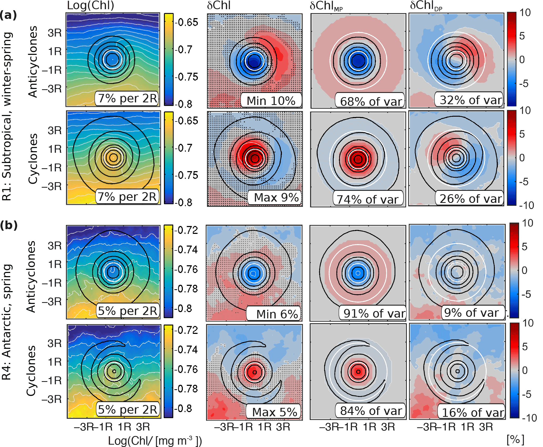
Figure 5Attribution of stirring/trapping components of mesoscale eddy associated Chl; (a) average instantaneous Chl and δChl (see Method Sect. 2.4) in region R1 (SSH larger 10 cm, June to November) and (b) in region R4 (SSH −140 to −100 cm, October), indicated as white boxes in Figs. 4b, c and 7. Within each subpanel, the top rows show the results for the anticyclones, and the bottom rows for the cyclones. The left column shows the logarithm (base 10) of Chl, the middle left the δChl (stippling marks insignificant anomalies), the middle right one the monopole component, MP, and the right one the residual component (approximately a dipole component, DP; see text for details and cartoon in Fig. 1). The sea level anomaly contours are shown in black (normalized before averaging); the inner and outer white circles indicate the eddy core and area used for the computation of the contribution to the variance of δChl of the monopole and the dipole, respectively; text in panels denotes (left) the meridional Chl gradient at two eddy radii, (second left) the maximum or minimum of the anomaly, (second right and right) the contribution to the variance of the anomaly pattern of the monopole and dipole, respectively; before averaging, the individual eddy snapshots are rotated according to the ambient instantaneous Chl gradient.

Download

Figure 6Attribution of stirring/trapping components; same as Fig. 5 but for (a) the region R2 (SSH −60 to −40 cm, January to May) and (b) for region R3 (SSH −50 to −15 cm, July to September). The regions are indicated with white boxes in Figs. 4b, c and 7.

Download

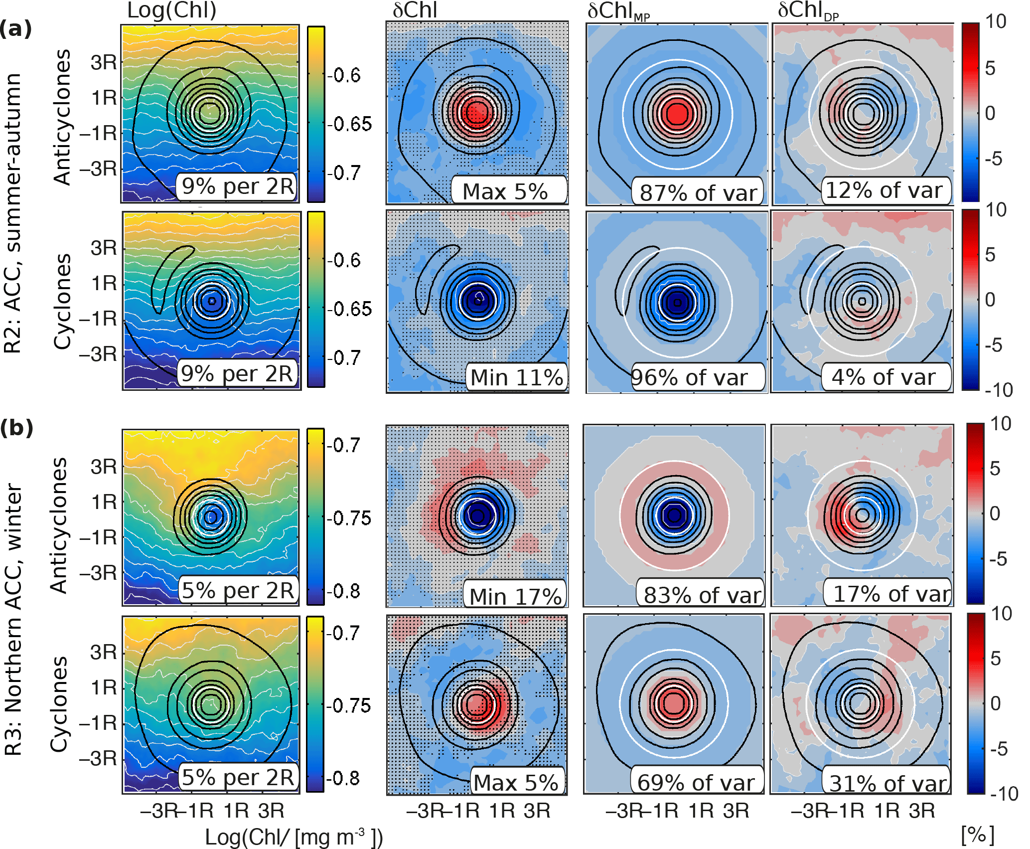
The advective potential for the other lateral advective mechanism, i.e., trapping, $\widehat{\mathit{\delta }}{\mathrm{Chl}}_{\mathrm{trap}}$, partly counteracts and partly enhances $\widehat{\mathit{\delta }}{\mathrm{Chl}}_{\mathrm{stir}}$ (Fig. 4d–g). For instance, for cyclones along the ACC from summer to autumn, trapping possibly contributes to a δChl signal (11 %) that is slightly larger than the Chl gradient at two eddy radii (9 %), and the contribution of the variance of the monopole is increased compared to anticyclones (Fig. 6a, 96 % versus 87 %). Yet, overall the trapping potential $\widehat{\mathit{\delta }}{\mathrm{Chl}}_{\mathrm{trap}}$ is weak compared to δChl (Fig. 4b, c, f, g), and outweighed by $\widehat{\mathit{\delta }}{\mathrm{Chl}}_{\mathrm{stir}}$.

3.2.2 Local biogeochemical rates

Even though advective processes, and particularly stirring, appear to be the dominant driver for the mesoscale eddy-associated Chl anomalies, there are nevertheless a few places where the magnitudes of the potentials for advective effects are too weak compared to the observed δChl or of opposite sign. These are the places where variations in the local growth and loss processes, i.e., variations in the local biogeochemical rates, may be the dominant driver.

The most prominent instance is found along the northern ACC, a region associated with the seasonal sign switch of δChl (Fig. 4b–g, blue boxes in Fig. 7a). Here, anticyclones switch to negative δChl in the presence of deep mixed layers, whereas both $\widehat{\mathit{\delta }}{\mathrm{Chl}}_{\mathrm{stir}}$ and $\widehat{\mathit{\delta }}{\mathrm{Chl}}_{\mathrm{trap}}$ suggest positive δChl. The shape of the local imprint of anticyclones in the respective region and season (Fig. 6b) indicates that the lateral Chl gradient at the scale of eddies (5 %) is small compared to the maximum absolute amplitude of δChl (17 %). Further, the decomposition of the local shape of δChl into a monopole and a dipole suggests that stirring (dipole) supports an anomaly of the opposite sign compared to the observed δChl, consistent with $\widehat{\mathit{\delta }}{\mathrm{Chl}}_{\mathrm{stir}}$ (Fig. 4d). Given that trapping would also cause a weak anomaly of the opposite sign (Fig. 4f), we hypothesize that eddy-induced changes in the biogeochemical rates are responsible for the negative δChl in winter and spring in the northern ACC.

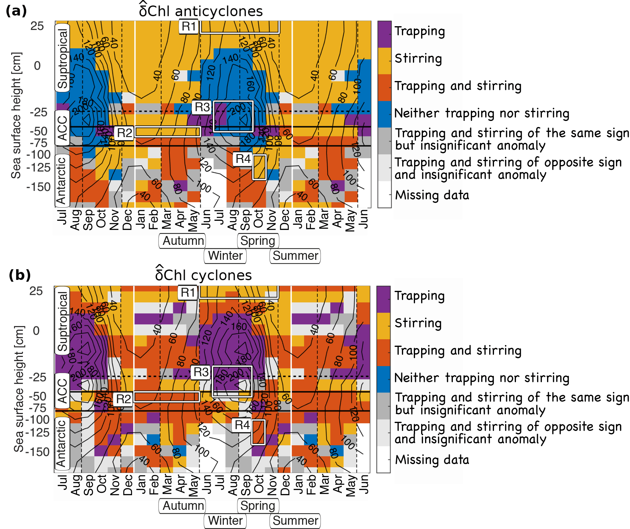
Figure 7Hovmoeller diagram of the processes likely controlling the chlorophyll anomalies (δChl) in (a) anticyclones and (b) cyclones: trapping (purple), stirring (yellow), a combination of the two (red) or neither of the two (blue), with the latter often interpreted to be the consequence of changes in the local growth or losses (biogeochemical rates). A region is colored if the sign of the potential effect is the same as the observed one, and if δChl is significant. See text for details. White boxes indicate regions R1 to R4 used for composite Figs. 5 and 6. The data were binned in monthly sea-surface height bins. Horizontal solid black lines mark the ACC, the horizontal dashed black line denotes the −20 cm SSH contour, the vertical dashed lines seasons; solid black contours show averaged mixed layer depths in meters; note that the seasonal cycle is shown repeatedly to highlight cyclic patterns.

Download

Figure 8Maps of the distribution of the processes likely controlling the chlorophyll anomalies (δChl) for austral (a) winter, (b) spring, (c) summer and (d) autumn for anticyclones (left) and cyclones (right). The method and legend is the same as used in Fig. 7. Otherwise the same as Fig. 2.

Download

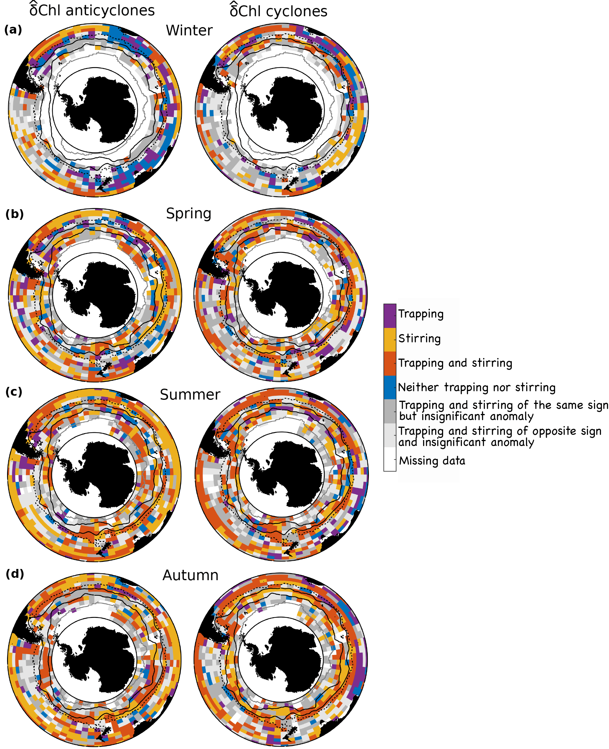
Similarly, the sign switch of δChl of cyclones in the same region cannot be explained based on $\widehat{\mathit{\delta }}{\mathrm{Chl}}_{\mathrm{stir}}$ (Fig. 4e). The local shape of Chl corroborates that for cyclones stirring of the average ambient Chl gradient also induces an anomaly of the opposite sign (Fig. 6b). In contrast to $\widehat{\mathit{\delta }}{\mathrm{Chl}}_{\mathrm{stir}}$, $\widehat{\mathit{\delta }}{\mathrm{Chl}}_{\mathrm{trap}}$ for cyclones is of the same sign as δChl (Fig. 4g), indicating a potential contribution of trapping to positive δChl under deep mixed layers. Yet, as noted in the previous paragraph, the magnitude of $\widehat{\mathit{\delta }}{\mathrm{Chl}}_{\mathrm{trap}}$ is small, hence the contribution by trapping is limited. Further, trapping is not of the same sign as δChl for cyclones everywhere in the region either (see blue boxes Fig. 8a,b, right column). Hence, the likely explanation for the δChl in cyclones in regions with deep winter mixed layers is that eddies also modify the local biogeochemical rates.

Effects of eddies on biogeochemical rates also may play a role in other regions or seasons. For instance, the magnitudes of $\widehat{\mathit{\delta }}{\mathrm{Chl}}_{\mathrm{stir}}$ and $\widehat{\mathit{\delta }}{\mathrm{Chl}}_{\mathrm{trap}}$ appear too weak to explain δChl in subtropical waters in winter and spring (Figs. 4d–g and 5a). Further, closed Chl contours are associated with the eddy cores that cannot originate from local lateral entrainment associated with stirring (Figs. 5 and 6, left columns). Also the generally weak potential $\widehat{\mathit{\delta }}{\mathrm{Chl}}_{\mathrm{trap}}$ fails to explain the closed Chl contours and the associated strong monopole component of δChl that contributes about 70 % to 100 % to the variability of the δChl shape (Figs. 4f, g, 5 and 6). These points both indicate that effects on biogeochemical rates enhance the δChl monopole.