Technical note: A refinement of coccolith separation methods: measuring the sinking characteristics of coccoliths

Zhang, Hongrui; Stoll, Heather; Bolton, Clara; Jin, Xiaobo; Liu, Chuanlian

doi:https://doi.org/10.5194/bg-15-4759-2018

Articles | Volume 15, issue 15

https://doi.org/10.5194/bg-15-4759-2018

Articles | Volume 15, issue 15

Technical note

09 Aug 2018

Technical note |

| 09 Aug 2018

Technical note: A refinement of coccolith separation methods: measuring the sinking characteristics of coccoliths

Hongrui Zhang, Heather Stoll, Clara Bolton, Xiaobo Jin, and Chuanlian Liu

Abstract

Quantification sinking velocities of individual coccoliths will contribute to optimizing laboratory methods for separating coccoliths of different sizes and species for geochemical analysis. The repeated settling–decanting method was the earliest method proposed to separate coccoliths from sediments and is still widely used. However, in the absence of estimates of settling velocity for nonspherical coccoliths, previous implementations have depended mainly on time-consuming empirical method development by trial and error. In this study, the sinking velocities of coccoliths belonging to different species were carefully measured in a series of settling experiments for the first time. Settling velocities of modern coccoliths range from 0.154 to 10.67 cm h⁻¹. We found that a quadratic relationship between coccolith length and sinking velocity fits well, and coccolith sinking velocity can be estimated by measuring the coccolith length and using the length–velocity factor, k_v. We found a negligible difference in sinking velocities measured in different vessels. However, an appropriate choice of vessel must be made to avoid “hindered settling” in coccolith separations. The experimental data and theoretical calculations presented here support and improve the repeated settling–decanting method.

How to cite

How to cite.

Dates

Received: 13 Feb 2018 – Discussion started: 27 Feb 2018 – Revised: 28 May 2018 – Accepted: 25 Jul 2018 – Published: 09 Aug 2018

1 Introduction

Coccolithophores are some of the most important phytoplankton in the ocean. They can secrete calcareous plates called coccoliths, which contribute significantly to discrete particulate inorganic carbon in the euphotic zone and to CaCO₃ fluxes to the deep ocean (e.g., Young and Ziveri, 2000; Sprengel et al., 2002). Coccolith morphology, geochemistry and fossil assemblage composition can reflect paleoenvironmental changes (e.g., Beaufort et al., 1997; Stoll et al., 2002; Zhang et al., 2016). However, the use of coccolith geochemical analyses in paleoenvironmental reconstructions has so far been impeded by the difficulty of isolating coccoliths compared with foraminifera. Two main methods have been developed to concentrate near-monospecific assemblages of coccoliths from bulk sediments: one is the method based on a decanting technique (Paull and Thierstein, 1987; Stoll and Ziveri, 2002) and the other is that based on micro-filtration (Minoletti et al., 2009). The improvement of separation techniques offered a new perspective to study the Earth's history (e.g., Stoll, 2005; Beltran et al., 2007; Bolton and Stoll, 2013; Rousselle et al., 2013). Moreover, the development of coccolith oxygen and carbon isotope studies in culture in recent years (e.g., Ziveri et al., 2003; Rickaby et al., 2010; Hermoso et al., 2016; McClelland et al., 2017) has provided an improved mechanistic understanding of coccolith isotope data and therefore stimulated the need for more purified coccolith fraction samples from the fossil record.

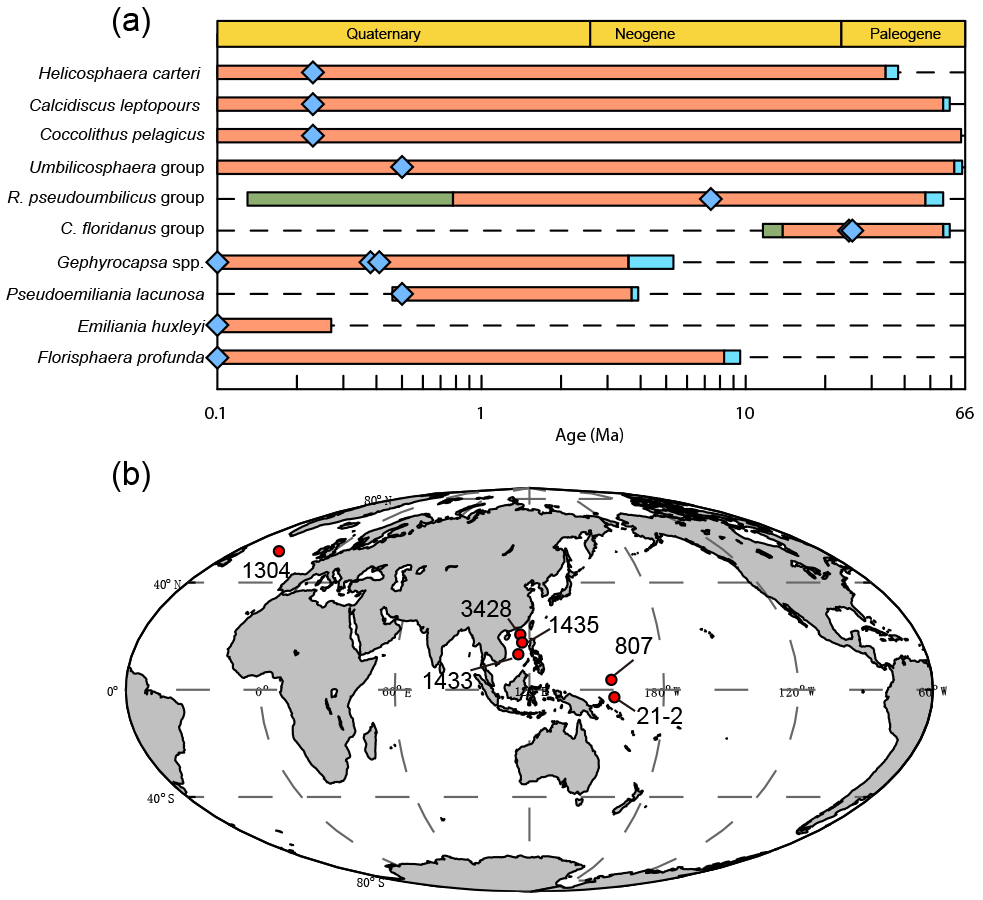
https://www.biogeosciences.net/15/4759/2018/bg-15-4759-2018-f01

Figure 1Temporal and spatial distribution of samples. (a) The evolution of studied coccoliths: first occurrence and last occurrence data are from Nannotax3 (http://www.mikrotax.org/Nannotax3/index.html). The blue bars represent ranges of first occurrence and the green bars represent ranges of last occurrence. The blue diamonds represent samples used in this study. (b) Spatial distribution of samples. Regarding the numbers on the map, 1304 means IODP U1304; 3428 means MD12-3428cq; 1433 and 1435 mean IODP U1433 and U1435, respectively; 807 means ODP 807, and 21-2 means KX21-2.

Download

Both decanting and micro-filtering are widely used methods for coccolith separation. The micro-filtering method separates coccoliths with a polycarbonate micro-filter membrane (with pore sizes of 2, 3, 5, 8, 10 and 12 µm). This method is highly effective in the larger size ranges but is very time-consuming in sediments with a high proportion of small (< 5 µm) coccoliths (which tends to be the case in natural populations). It is also impossible to separate coccoliths such as Florisphaera profunda and Emiliania huxleyi with similar lengths by micro-filtration (Hermoso et al., 2015). Decanting, on the other hand, is highly effective for the small-sized coccoliths, because their slow settling times permit a greater ability to separate different sizes. Consequently, in some studies, a combination of the micro filtering and sinking or centrifugation method were applied for coccolith separation (Stoll, 2005; Bolton et al., 2012; Hermoso et al., 2015). The repeated sinking–decanting method, first employed by (Edwards, 1963; Paull and Thierstein, 1987) follows the simple principle formalized by Stokes' law for spherical particles: particles of a larger size settle more quickly because they have a higher ratio of volume and mass (accelerating sinking) to sectional area (resistance retarding sinking). However, the sinking velocities of coccoliths with a complex shape are difficult to calculate and have not been quantified in previous studies. Consequently, the repeated decanting method has generally used settling times based on empirical trial and error.

In the current study, we present a novel and rigorous estimation of sinking velocity for 16 species of modern and Cenozoic coccoliths, carefully measured in 0.2 % ammonia at 20 ^∘C. With this new dataset, we explore how to estimate the sinking velocity of coccoliths based on their shape and length, which allows our estimations to be generalized for other species and for situations where the mean length of coccoliths of a given species was different from that of our study. These generalizations, together with our results on sinking velocities of one coccolith species (Gephyrocapsa oceanica) in different vessels, should allow a significant improvement in the efficiency of future protocols for the separation of coccoliths by repeated decanting.

2 Materials and methods

2.1 Sample selections

We measured the sinking velocity of 16 different species of coccoliths, isolated from eight deep-sea sediment samples from the Pacific and Atlantic oceans (Fig. 1, Table A1 in Appendix). Sample were principally of Quaternary age but include two Neogene/Paleogene samples. In general, numbers of small coccoliths, including E. huxleyi, Gephyrocapsa spp. and Reticulofenestra spp., are about 1 order of magnitude greater than that of larger coccoliths. However, the larger coccoliths' contributions to carbonate can be as high as 50 % (Baumann, 2004; Jin et al., 2016). Moreover, both small coccoliths and large coccoliths are useful in geochemical analyses (Ziveri et al., 2003; Rickaby et al., 2010; Candelier et al., 2013; Bolton et al., 2012, 2016; Bolton and Stoll, 2013). Therefore, both small and large coccoliths were studied in this research. Pictures of the studied coccolith are shown in Appendix B, and all classifications follow Nannotax3 except Reticulofenestra spp. (Fig. C2 in Appendix C).

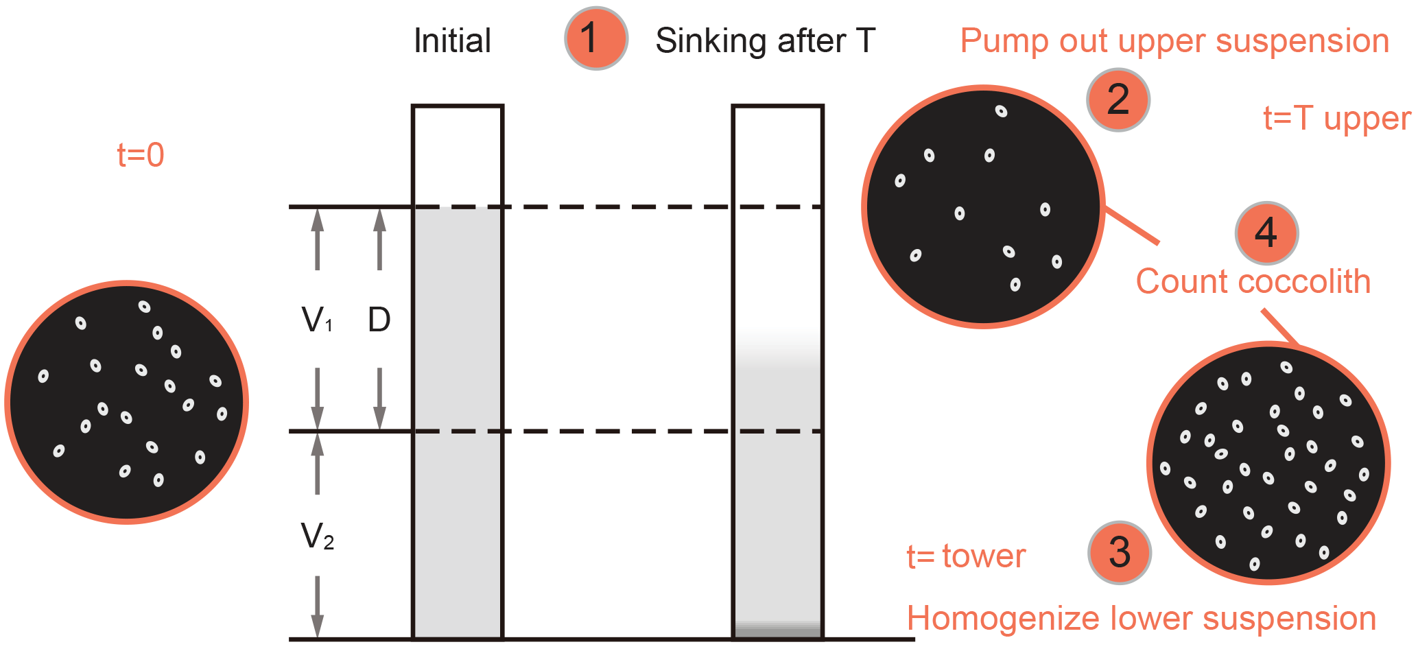
https://www.biogeosciences.net/15/4759/2018/bg-15-4759-2018-f02

Figure 2Schematic of settling experiments. V₁ and V₂ are the volumes of the upper and lower cylinders; D is the settled distance. The numbers in circles are same as the number of steps described in Sect. 2.2.1.

Download

2.2 Experiment designs

2.2.1 Sample pretreatments

The sinking velocity measurement depends on absolute abundance estimation (more details in Sect. 2.2.2). However, on microscope slides, larger coccoliths and foraminifer fragments may cover smaller coccoliths, reducing the accuracy of coccolith absolute numbers. Thus, before sinking experiments were carried out, raw sediments were pretreated to purify the target coccoliths to reduce errors in coccolith counting. The raw sediments were disaggregated in 0.2 % ammonia and sieved through a 63 µm sieve and then treated by the sinking method or the filtering method (Bolton et al., 2012; Minoletti et al., 2009) to concentrate the target species up to at least more than 50 % of the total assemblage (for Noelaerhabdaceae coccoliths, a percentage of more than 90 % can be easily achieved). In one sample with aggregation (ODP 807), we did a rapid settling (30 min, 2 cm) to eliminate aggregates. Most of the species were measured individually in settling experiments, except for Pseudoemiliania lacunosa and Umbilicosphaera sibogae, which were measured together.

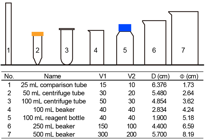
https://www.biogeosciences.net/15/4759/2018/bg-15-4759-2018-f03

Figure 3The shape parameters of vessels. V₁ and V₂ means the volume of upper suspension and lower suspension, respectively. D means sinking distance. Φ means average inner diameter, which is calculated by $2 (V_{1} / π D)^{- 2}$ .

Download

2.2.2 Measuring the sinking speeds of coccoliths

We are not aware of any prior direct determination of the sinking velocity of individual coccoliths, although the sinking velocities of live coccolithophores and other marine algal cells have been successfully measured by the FlowCAM method (Bach et al., 2012) or a similar photography technique (e.g., Miklasz and Denny, 2010). Here, we introduce a simple method to measure the particle sinking speeds without special equipment.

After pretreatment, the coccolith suspensions were gently shaken and then moved into comparison tubes which were vertically mounted on tube shelves. We set the timer going and let the suspension settle for a specified period of time, marked as sinking time or settling duration (T).
Thereafter, we removed the upper 15 mL supernatant into a 50 mL centrifuge tube with a 10 mL pipette. This operation was performed slowly and gently to avoid drawing lower suspensions upward. The absolute counting of coccolith was achieved by using the “drop technique” to make quantitative microscope sides (Koch and Young, 2007; Bordiga et al., 2015). In total, 0.3 mL mixed suspension was extracted with pipettes onto a glass cover, and the slider was dried on a hotplate.
The lower suspension was than homogenized and another slider was prepared as described above.
The number of coccoliths in the upper and lower suspensions were carefully counted on microscope at ×1250 magnification and the number of coccoliths and fields of view (FOV) were recorded for further calculations. More than 300 specimens were counted for most of the measurements. For the Helicosphaera carteri measurements, more than 100 FOV were checked and about 100 specimens were counted.

To calculate the sinking velocities of coccoliths, we define a parameter named the separation ratio (R), which represents the percentage of removed coccoliths in one separation by pumping out the upper suspension. This parameter is important and will be repeatedly mentioned in the following part. R was measured using the following equation (more details about derivation can be found in Appendix D):

\begin{matrix} (1) & R = \frac{\frac{N 1}{n 1} \times V_{1}}{\frac{N 1}{n 1} \times V_{1} + \frac{N 2}{n 2} \times V_{2}}, \end{matrix}

where N₁ and N₂ are numbers of coccoliths counted on upper and lower suspension slides, respectively; n₁ and n₂ are the number of FOV counted. V₁ and V₂ are the volume of the settling vessel defined by the settling distance, as shown in Fig. 2.

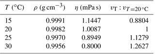
Table 1The influence of temperature on sinking velocity. Density data are from Kell (1975), and viscosity data are from Kestin et al. (1978).

Download Print Version | Download XLSX

The separation ratio, R, also has a relationship with sinking time, T (Appendix D):

\begin{matrix} (2) & R = \frac{V_{1} - \frac{V_{1}}{D} \times v \times T}{V_{1} + V_{2}}, \end{matrix}

where V₁, V₂ and D are the shape parameters shown in Fig. 2 and v is the average sinking velocity of measured coccoliths. If we plot R against T, the slope of the line has a relationship with v. Then linear regressions between R and T were processed with MATLAB to calculate the v (details about error analyses can be found in Appendix E).

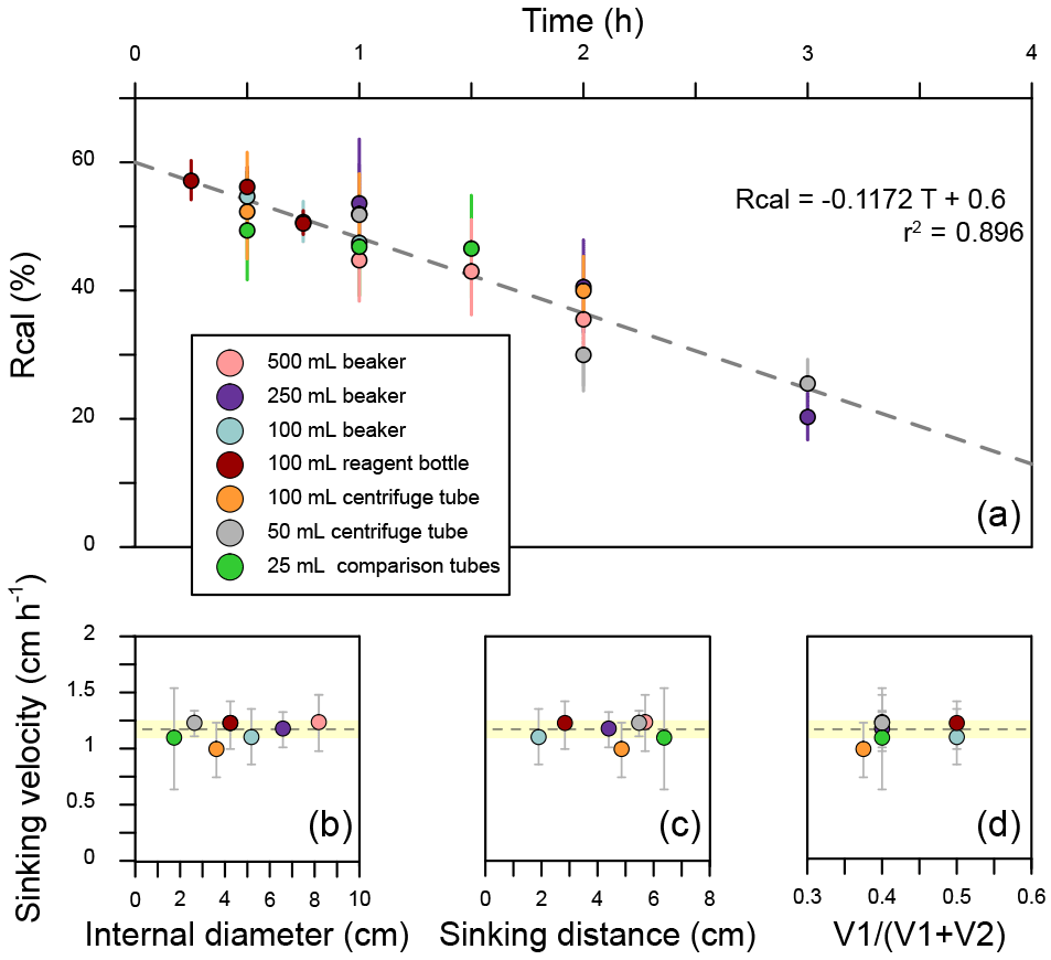
https://www.biogeosciences.net/15/4759/2018/bg-15-4759-2018-f04

Figure 4Sinking velocities of G. oceanica in the core KX-21-2 measured in different vessels. (a) The calibrated separation ratios measured in different vessels. Error bars show 95 % confidence level of calibrated separation ratio. (b–d) The relationship between sinking velocity and different vessel shape parameters. Error bars represent 95 % confidence level of sinking velocity in each vessel, and the shaded area represents the 95 % confidence level of sinking velocity considering all data points.

Download

There are still two issues to be explained. Firstly, to eliminate the shape differences among vessels, all separation ratios have been transferred to calibrated separation ratios (R_cal), which means the separation ratio measured in a standard vessel with V₁=15 mL, V₂=10 mL and D=6 cm (more details about transformation from R to R_cal can be found in Appendix D). Secondly, we treated the average sinking velocities as the sinking velocities of the coccoliths with the average length. This approximation is proved reasonable in Appendix D.

2.2.3 Detecting the potential influence of vessels

Seven commonly used vessels were selected to detect the potential influence of vessels (Fig. 3). Two of them are made of plastics (no. 2 and no. 3 in Fig. 3), and all others are pyrex glass vessels. About 500 mg of sediment from core KX21-2 were pretreated as described in Sect. 2.2.1 and suspended in about 500 mL diluted ammonia. After that, settling experiments were performed as described in Sect. 2.2.2 using different vessels. In these experiments, only the dominant species, G. oceanica, was measured.

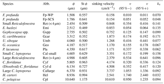
Table 2The sinking velocity and shape–velocity factor of different coccolith species: ϕ means the distal shield length of coccolith and St ϕ is the standard deviation of distal shield length; sv represents the sinking velocity; v (95 %−) and v (95 %+) represent the lower and higher limit of 95 % confidence level, respectively; k_v represents the length-sinking velocity factor. The abbreviated name of coccoliths can be found in the caption of Fig. 4. The details of coccolith length distribution are found in Appendix C.

Download Print Version | Download XLSX

2.2.4 Other factors influencing the sinking velocity

Temperature can change the density and viscosity of liquid. Generally speaking, the higher the temperature is, the lower the density and viscosity will become and the faster pellets will sink. Take water, for instance: if the temperature increases from 15 to 30^∘, the particle sinking velocity will increase by ∼43 % (Table 1). All sinking velocities measured or discussed in the following sections were velocities at 20 ^∘C to minimize the influence of temperature.

https://www.biogeosciences.net/15/4759/2018/bg-15-4759-2018-f05

Figure 5The calibrated ratio (R_cal) vs. sinking duration. Fp-WP means F. profunda in the West Pacific. Fp-SCS means F. profunda in the South China Sea. Emi means E. huxleyi. Gspp means small Geophyrocapsa. Geo means G. oceanica. Gcarb means G. caribbeanica. Ret < 4 means small Reticulofenestra. Ret > 4 means large Reticulofenestra. Cyf means Cyclicargolithus floridanus. Cy-d means dissolved C. floridanus. Umb means U. sibogae. Pla means Pseudoemiliania lacunosa. Hel means H. carteri. Cal large means larger Calcidiscus leptoporus. Cal small means small C. leptoporus. Cpl means C. pelagicus.

Download

The calibration of sinking velocity in high-concentration suspension has been calculated by Richardson and Zaki (1954):

\begin{matrix} (3) & v = v_{0} (1 - α_{s})^{2.7}, \end{matrix}

where the α_s is the solids volume fraction. Based on Eq. (3), the higher the suspension concentration is, the slower the sinking velocity will be. This is so-called “hindered settling”. When the α_s=0.2 %, the reduction in sinking velocity owing to hindered settling is negligible (v∕v₀ equals 99.46 %). Hence, in this study all suspensions have solid volume fractions lower than 0.2 % to avoid notable reductions in coccolith sinking velocities.

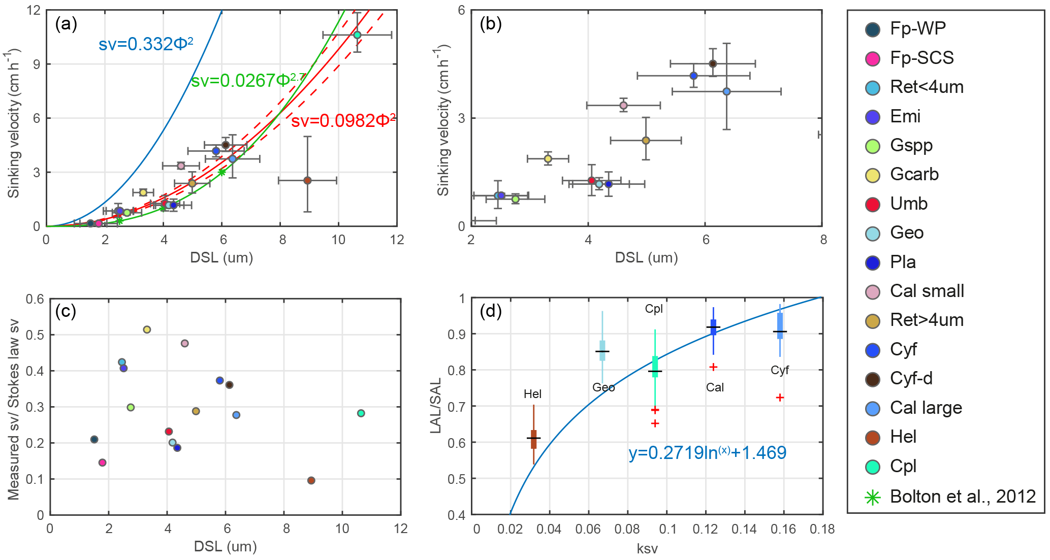
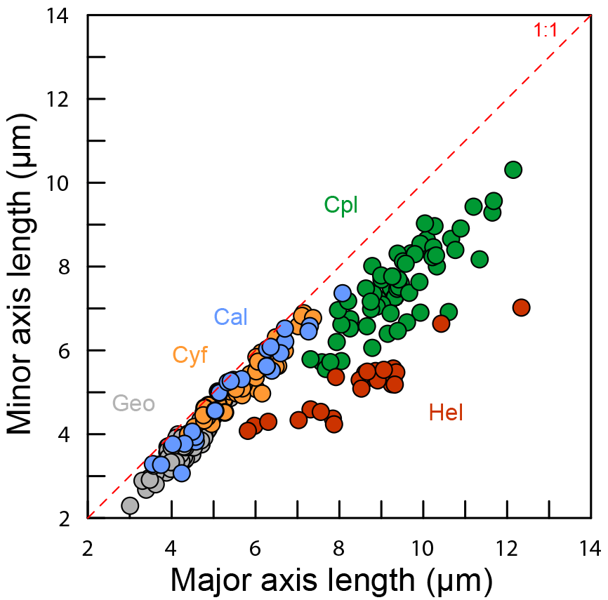
https://www.biogeosciences.net/15/4759/2018/bg-15-4759-2018-f06

Figure 6Coccolith sinking velocities and coccolith shape factors. (a–b) Sinking velocities and mean distal shield length. The horizontal error bars represent 1 standard deviation of coccolith length, and the vertical ones represent the 95 % confidence level of measured the sinking velocities. The blue, green and red lines represent sinking velocity of calcite sphere objects, coccolith sinking velocities estimated by Bolton et al. (2012) and this study, respectively. (c) The ratio of measured speed and speed calculated by Stokes' law. (d) Coccolith short axis length (SAL) and long axis length (LAL) ratio against shape–velocity factor k_v. Box shows median value and upper/lower quartiles, whiskers show maximum and minimum values; outliers larger than 1.5 of the interquartile range are shown as red crosses. The SAL against LAL plot was shown in Fig. C3. The short names of coccoliths can be found in Table 2.

Download

3 Results and discussions

3.1 Influence of vessels

The sinking velocities of G. oceanica in the core KX21-2 in 0.2 % ammonia at 20 ^∘C measured in different vessels vary from 0.99 to 1.23 cm h⁻¹. The lowest value occurred in the 100 mL centrifuge tube and the highest sinking velocity was measured in the 50 mL centrifuge tube experiments. The correlations between sinking velocities and different vessel parameters are quite low: r=0.13 for the vessel inner diameter, r=0.0005 for the sinking distance, and r=0.051 for the upper volume and total volume ratio ( $V_{1} / (V_{1} + V_{2})$ ). The dissipation of energy by friction between the moving fluid and the walls can cause a reduction in sinking speed (wall effect). A significant wall effect will be detected when a particle is settling in a vessel with a diameter that is smaller than 100 times the particle size (Barnea and Mizarchi, 1973). The length of coccoliths is on the micron scale, so the diameters of vessels used in the laboratory are more than 4 orders of magnitude larger than coccoliths. Moreover, our results show that the difference between vessel materials, glass and plastics can also be ignored (Fig. 4). Hence, we suggest that vessel type almost has no significant influence on the sinking velocity of coccoliths.

However, our experiments were premised on the basis that the concentration of suspension was equal among different vessels. This means that large vessels can treat more sediment at one time, but if we choose a larger vessel, we need to spend more time in pumping suspensions, and it often costs more time in terms of sinking (often due to longer sinking distance). Assuming that the sediment is composed of 50 % calcite (with a density of 2.7 g cm⁻³) and 50 % clay (about 1.7 g cm⁻³), the largest amount of sediment that can be used without a significant reduction in the sinking velocity (5 %) is about 400 mg in 100 mL suspension (this calculation is based on Eq. 3). However, because sediments accumulate in the lower suspension, the particle concentration can be more than 4 times higher than in the initial homogenous concentration. This phenomenon will be more significant for a vessel with a narrow bottom, such as centrifuge tubes. To avoid this, we recommend using about 100 mg dry sediment suspended in at least 100 mL suspension to avoid hindered settling. If more sediment is necessary for geochemistry analyses, then a larger vessel should be selected to separate enough sample at one time.

https://www.biogeosciences.net/15/4759/2018/bg-15-4759-2018-f07

Figure 7The selection of separation velocities: the sinking velocities of three main coccolith species in sample from core KX21-2 were calculated by the length distribution and velocity factors in Table 2. The yellow dots represent sinking velocities of coccoliths with mean length. The edge of boxes show the sinking velocities of coccoliths within 1 standard deviation of length (±1σ), and the whiskers mark the sinking velocities of coccolith within 2 standard deviations of length (±2σ).

Download

3.2 Sinking velocities at 20 ^∘C in 0.2 % ammonia

We measured the separation ratios of different coccoliths in comparison tubes at 20 ^∘C in 0.2 % ammonia (Fig. 5). The sinking velocities of coccoliths were then calculated by linear fitting of separation ratios and settling durations. The sinking velocities of studied coccoliths vary by 2 orders of magnitude from 0.154 to 10.67 cm h⁻¹ (Table 2). The highest sinking velocity was found in the measurement of Coccolithus pelagicus, and the lowest velocity was found for F. profunda. The average sinking speed of coccoliths is about 10 %–50 % of the terminal sinking velocities of calcite spheres calculated by Stokes' law (Fig. 6c). These ratios are comparable to the oval-object (e.g., seeds) data from Xie and Zhang (2001) and smaller than the steel-ellipsoid data from McNown and Malaika (1950). The sinking velocities of coccoliths measured in our experiment are about 2–3 orders of magnitude smaller than values from sediment traps of 143–243 m d⁻¹ (595 ∼1012 cm h⁻¹) in the North Atlantic (Ziveri et al., 2000; Stoll et al., 2007), suggesting that the coccoliths sinking out of the euphotic layer are mainly in the form of sinking aggregates rather than individual coccoliths.

3.3 Estimating the sinking velocities

Generally speaking, the sinking velocities of coccoliths increase with distal shield length (Fig. 5a), as expected from the increase in volume to sectional area for a given geometry as length increases. Our data imply that the sinking velocity has a power function relationship with distal shield length.

We propose that the sinking velocity of coccoliths might have a quadratic relationship with distal shield length as described by Stokes' law (Fig. 6a). If we use data for all species except H. carteri (the reason can be found in the following discussion), the sinking velocities can be described by the following equation:

\begin{matrix} (4) & v = 0.098 (\pm 0.001) \times ϕ^{2} . \end{matrix}

Based on this quadratic regression, we derive a shape–velocity factor (k_v) that relates settling velocity to coccolith length.

\begin{matrix} (5) & v = k_{v} \times ϕ^{2} \end{matrix}

Furthermore, this factor is analogous to the shape–mass factor, k_s, used to relate coccolith mass to coccolith length (Young and Ziveri, 2000). The length and shape–velocity factor of coccoliths can be used to predict most of the sinking velocity variations; however, variations may also arise due to changes in coccolith mass and thickness, for a given length, and due to the hydrodynamics of particular shapes. We noticed that the smaller coccolith G. caribbeanica has a greater sinking velocity than the larger coccolith, G. oceanica. We suggest that this was caused by greater mass per length (or greater average thickness) in the case of G. caribbeanica, and this may be due to the closed central area while G. oceanica has an open central area. Another example is H. carteri, the lower sinking velocity of which can be explained by the unique structure of H. carteri coccolith. Firstly, the broad edge of H. carteri can increase the drag force significantly. Moreover, most of the measured coccoliths have a ellipticity (major axis length and minor axis length ratio) larger than 0.8, while the ellipticity of H. carteri is around 0.6, which means the mass of H. carteri is smaller than other species of coccoliths with similar lengths (Figs. 6d and C3). That is also the reason H. carteri was excluded from the general regression in Eq. (4). In the case of partial dissolution, the well-preserved Cyclicargolithus floridanus may have higher mass than dissolved (or disarticulated) C. floridanus and therefore a slightly higher shape–velocity factor.

4 Suggestions for coccolith velocity estimations and separations

To improve coccolith separation by settling methods, we measured sinking velocities of different coccoliths by gravity. Sinking velocities in this study varied from 0.154 to 10.61 cm h⁻¹, about 10 % to 50 % of those of calcite spheres with the same diameter. The shape of different vessels had little impact on the sinking velocity. But we should consider the volume of vessels to avoid hindered settling. The sinking velocities are mainly controlled by the shape of coccoliths, including the distal shield length, the size of the central area and the ellipticity of coccoliths. Besides the shape of coccoliths, temperature is also crucial to the coccolith separations because of the dependence of sinking velocities on temperature. Length–velocity factors were proposed to estimate coccolith sinking velocities, so coccolith separation can be achieved by the following steps:

Measure the length of coccoliths in your target assemblage under the microscope and regress the length distribution by the assumption of a normal distribution (details are in Appendix C).
Estimate sinking velocities for each important species. For species whose sinking speed has been directly measured, we can use the length–velocity factor directly ( $v = k_{v} \times ϕ^{2}$ ). For unmeasured species, we can choose the length–velocity factor of coccoliths with a similar morphology in this study or use the general length–velocity formula ( $v = 0.098 (\pm 0.001 \times ϕ^{2}$ ).
Calculate the separation time for the main species. For example, in KX21-2 there are three main coccoliths (F. profunda, G. oceanica and C. leptoporus), and we wish to separate G. oceanica out from the bulk sediment. Calculate each coccolith's sinking velocity distributions as described in Step 2 above. As shown in Fig. 7, a sinking velocity intermediate between F. profunda (with a length 2σ larger than average, marked as +2σ) and G. oceanica (with a length 2σ smaller than average, marked as −2σ), optimal for separating them, would be 0.6 cm h⁻¹. Similarly, we can chose speed thresholds of 1.85 cm h⁻¹ to separate G. oceanica from C. leptoporus. If we settle in a 50 mL centrifuge tube with a sinking distance, D, equal to 5.84 cm, the sinking time for separating F. profunda should be $T = 5.84 / 0.6 = 9.73$ h. Similarly, we can calculate the time for separating G. oceanica by $T = 5.84 / 1.85 = 3.16$ h.
Homogenize the sediment suspension and let coccoliths settle for the period calculated in Step 3. After that, pump out the upper part of the suspension. In the upper part, we exclusively have the smaller of the main coccoliths. However, the column will still contain some smaller ones. So this step (settling and pumping) should be repeated until the lower part no longer has any significant contribution from the smaller coccoliths. This step has been described well in previous studies, and more details can be found in Stoll and Ziveri (2002) and Bolton et al. (2012).

We find that, if we use the general formula, a closed central area coccolith will sink faster than predicted (G. caribbeanica and small C. leptoporus will settle ∼40 % faster) and coccoliths with greater ellipticity can settle much more slowly (H. carteri will settle as 30 % of the predicted sinking velocity for coccoliths with similar length). Moreover, the sinking method cannot separate every species of coccoliths perfectly. As mentioned in Sect. 2.2.1, P. lacunosa and U. sibogae cannot easily be separated from each other because they have similar sinking velocities. Nevertheless, this study provides the first direct estimation of coccolith settling velocities, which should simplify the implementation of future methods to separate coccoliths by settling time.

Data availability

The sinking velocities and coccolith length results can be found in Table 2.

Appendix A: Sample selections

Table A1Sample selections. SCS represents the South China Sea; W. P. represents the western Pacific; N.A. represents the northern Atlantic.

Download Print Version | Download XLSX

Appendix B: Coccolith images under circular polarized light

https://www.biogeosciences.net/15/4759/2018/bg-15-4759-2018-f08

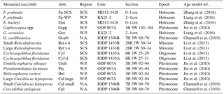
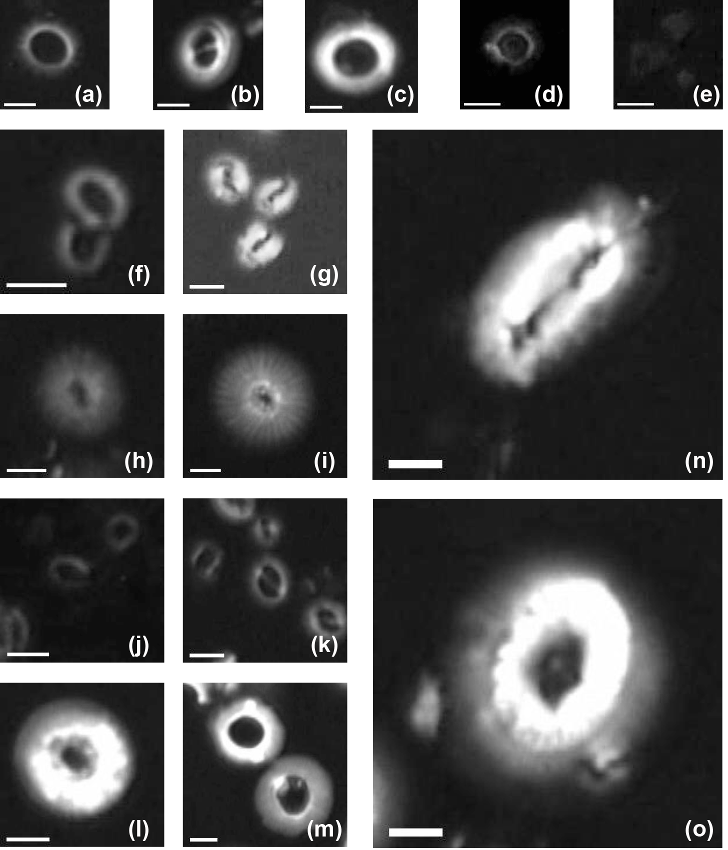
Figure B1Imaged of coccoliths measured in this study: (a) Pseudoemiliania lacunosa in the core ODP 807; (b) Gephyrocapsa oceanica in the core KX21-2; (c) Reticulofenestra spp. (large) in the core IODP U1433B; (d) Umbilicosphaera sibogae in the core ODP 807; (e) Florisphaera profunda in the core KX21-2; (f) Reticulofenestra spp. (small) in the core IODP U1433B; (g) Gephyrocapsa caribbeanica in the core IODP U1304B; (h) small Calcidiscus leptoporus in the core IODP U1304B; (i) large Calcidiscus leptoporus in the core ODP 807A; (j) Emiliania huxleyi in the surface sediment in the South China Sea; (k) Gephyrocapsa spp. in the core ODP 807; (l) Cyclicargolithus floridanus in the core IODP U1435A and (m) dissolved Cyclicargolithus floridanus in the same core; (n) Helicosphaera carteri in the core ODP 807A; (o) Coccolithus pelagicus in the core IODP U1304B. White bars represent a length of 2 µm.

Download

Appendix C: The length distribution of coccoliths

To measure the distal shield length of coccoliths, pictures were taken at a magnification of 1250× under circular polarized light. The coccolith lengths were measured by using the image analysis software, ImageJ. More than five pictures were taken, and more than 50 (usually more than 100) coccolith specimens were measured. The length distributions of coccoliths measured in our experiments are shown in Fig. C1.

https://www.biogeosciences.net/15/4759/2018/bg-15-4759-2018-f09

Figure C1Size distribution of coccoliths measured in the present study. The abbreviations of coccolith names follow Table A1.

Download

The classification of coccoliths by length was supported by mixture analysis in PAST (Hammer et al., 2001), such as Reticulofenestra spp. and Gephyrocapsa spp. Reticulofenestra spp. in the Miocene were classified into two groups, Ret. (< 4 µm) and Ret. (> 4 µm). The traditional classification of Reticulofenestra spp. is < 3, 3–5 and 5–7 µm did not pass the normal distribution test. Hence, in this study the Reticulofenestra spp. are divided at 4 µm (Fig. C2). Gephyrocapsa spp. were divided by the shape (length and central area) of coccoliths into small Gephyrocapsa (central area opening and length < 3.5 µm), G. oceanica (central area opening and length > 3.5 µm) and G. caribbeanica (closed central area).

https://www.biogeosciences.net/15/4759/2018/bg-15-4759-2018-f10

Figure C2The classical classification of Reticulofenestra spp. (a) and the classification used in our study (b). The curves represent the normal distribution fits of different coccolith groups, and the dashed curve marks that the goodness of fit is below 0.2.

Download

https://www.biogeosciences.net/15/4759/2018/bg-15-4759-2018-f11

Figure C3The short axis and long axis length distribution of coccoliths in Fig. 6d.

Download

Appendix D: Coccolith movement in gravity settling

In this part, the derivation of the equation will be explained in detail including proofs of several assumptions mentioned in the Materials and methods section.

When the well-mixed sediment begins to sink, the decrease in coccolith number in the upper suspension (N_u) can be described by the following equation:

\begin{matrix} (D1) & \frac{d N_{u}}{d T} = - \frac{N_{u (t = 0)}}{D} \times v, \end{matrix}

where the D is the length of upper suspension and $N_{u (t = 0)} / D$ is the initial number of coccoliths in a cross section with a unit thickness; v is the mean sinking velocity of coccolith. In practice, the velocities of coccoliths are different, so we assume that the measured velocity is the mean sinking velocity of bulk coccolith. This assumption will be proved valid in the following. The particle can reach 99.9 % of the maximum sinking velocity within only 10⁻⁷ s, so we assume that the particle sinks with maximum velocity from when it begins to settle.

Through integrating Eq. (D1), we can get the variation in coccolith number in the upper column over time:

\begin{matrix} (D2) & N_{u} = N_{u (t = 0)} - \frac{N_{u (t = 0)}}{D} \times v \times T, \end{matrix}

where T is settling time. After a period of time (T), we pump out the upper suspension. Here, we define the number of coccoliths in the upper supernatant dividing the total coccoliths number in the tube (N_t) as the separation ratio (R), which represents the percentage of total coccoliths removed in one separation. R can be expressed by

\begin{matrix} (D3) & R = \frac{N_{u}}{N_{t}} . \end{matrix}

Assuming all coccoliths are uniformly distributed in the suspension at the beginning of settling, N_u(t=0) has the following relationship with N_t:

\begin{matrix} (D4) & \frac{N_{u} (t = 0)}{N_{t}} = \frac{V_{1}}{V_{1} + V_{2}}, \end{matrix}

where V₁ is the volume of upper suspension and V₂ is the volume of lower suspension.

Combining the Eqs. (D1), (D2), (D3) and (D4), we obtain the relationship between the separation ratio, R, and sinking velocity, v, as follows:

\begin{matrix} (D5) & R = \frac{N_{u}}{N_{t}} = \frac{N_{u (t = 0)} - \frac{N_{u (t = 0)}}{D} \times v \times T}{N_{t}} = \frac{V_{1} - \frac{V_{1}}{D} \times v \times T}{V_{1} + V_{2}} . \end{matrix}

If we plot R and T on a figure, the slope of the line is a function of V₁, V₂, D and v. Since V₁, V₂ and D are known parameters, we say the slope of R−T is a function of v, which is exactly what we want.

The comparison tubes used in our experiments have the same V₁ and V₂ but different D. Other vessels used in other experiments have different V₁, V₂ and D. So we should adjust the raw separation ratio to the calibrated separation ratio (R_cal), which represents the separation ratio in a standard vessel with V_1 SD=15 mL, V_2 SD=10 mL and D_SD=6 cm. This step can be described by Eq. (D6):

\begin{matrix} (D6) & R_{cal} = \frac{[R \times (V_{1} + V_{1}) - V_{1}] \times D \times V_{1 SD}}{(D_{SD} \times V_{1} + V_{1 SD}) \times (V_{1 SD} + V_{2 SD})} . \end{matrix}

After calibration, the slope of R_cal−T (k) has the following relationship with v:

\begin{matrix} (D7) & v = - \frac{D_{SD} \times (V_{1 SD} + V_{2 SD})}{V_{1 SD}} \times k = - 10 \times k, \end{matrix}

where k is the slope of R_cal against T from regression and other parameters are as described above. Hence, the sinking velocity of different coccoliths can be achieved by measuring the variations in R_cal over time.

The coccoliths' lengths in the sediment have some variations. So what we measured is actually the bulk settling velocity of the whole coccolith population. We also offer a test for the assumption that the average sinking velocity of all coccoliths can be treated as the sinking velocity of coccoliths with the average length. Here, we used the data of G. oceanica. A normal distribution was fitted to the measured length distribution (Fig. D1a). We generated 100 000 coccolith following the normal distribution, and let these coccolith evenly distribute in the comparison tube at the beginning and then allowed them to sink without colliding with each other. The sinking velocities of different size coccoliths were calculated by the velocity–shape parameter k_v as described in the Results and discussions section. We modeled the coccoliths sinking process and computed the separation ratio (red dashed line in Fig. D1b), coccolith length (red dashed line in Fig. D1c) and instant sinking velocities (orange dots in Fig. D1d) at different time sections.

For G. oceanica experiments, the instant sinking velocity would not change significantly until settling for more 3 h. That means for all R_cal larger than 15 % are safe for linear regressions. The minimum safe number of R_cal will decrease with the drop of dispersion degree of the coccolith length distribution. Hence, our assumption of average sinking velocity and the use of linear regression are proved to be reasonable.

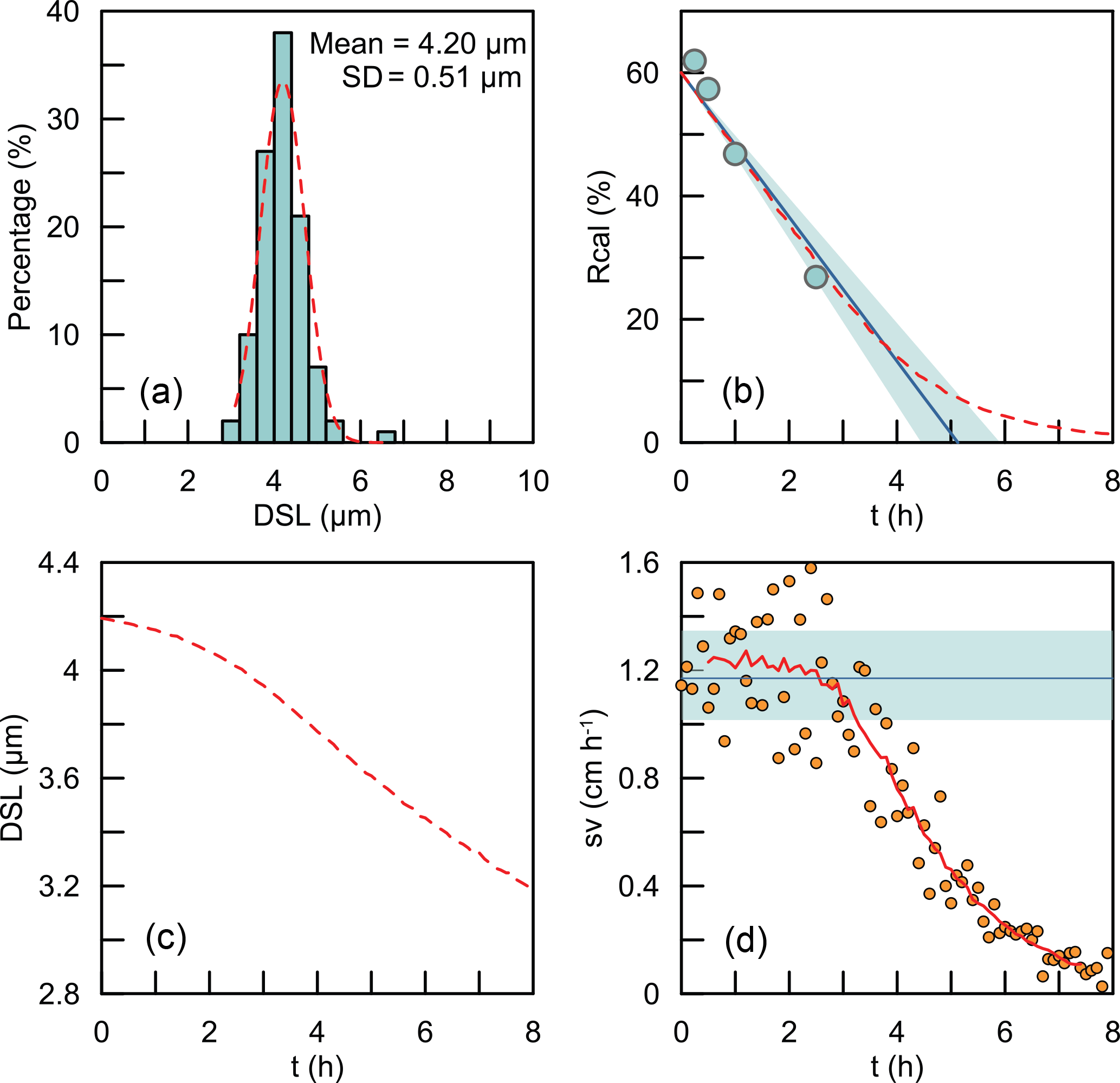
https://www.biogeosciences.net/15/4759/2018/bg-15-4759-2018-f12

Figure D1The simulations of coccoliths settling with different lengths: (a) the length distribution of coccoliths. The green bars represent measured data, and the red dashed line represents the best fit for the normal distribution. (b) The calibrated separation ratio: the green dots are data measured in our settling experiments, the blue line and shaded area represent the calculated sinking velocity based on R_cal measurement, and the red dashed line represents results obtained from simulations. (c) The average length of coccoliths removed in simulations. (d) The modeling sinking velocities of coccoliths: the orange dots are the instant sinking velocity calculated from the derivation of R_cal; the red dashed line is the weighted average for the instant sinking velocity. The blue line represents the average sinking velocity we measured, and the green shaded area represents the 95 % confidence level of the measured velocity.

Download

Appendix E: Statistical and error analyses

The errors of the measured separation ratio (R) and calculated sinking velocity (v) are mainly caused by counting coccoliths, the error of which follows the Poisson distribution. To detect the influence of counting number on the result error, the error of the separation ratio was simulated by 5000 Monte Carlo calculations with assumptions that $V_{1} : V_{2} = 15 : 10$ and n₁=n₂ (Fig. E1). The result shows that the number of coccoliths counted in the upper column has greater influence on the relative error ( $| R - R_{95 CL} | / R$ ). That means more coccoliths in the upper suspension should be counted to make results more accurate. The slope of R_cal−T was calculated by linear fitting with the intercept fixed on $V_{1} / (V_{1} + V_{2}$ ). The input R_cal were generated from measured values considering the error of coccolith counting (by the Matlab function “random”). The regressions of R_cal−T were repeated by 5000 regressions in the software Matlab (by the function “lsqcurvefit”), and the error of sinking velocity, v, was taken from the distribution slope of R_cal−T in the Monte Carlo process.

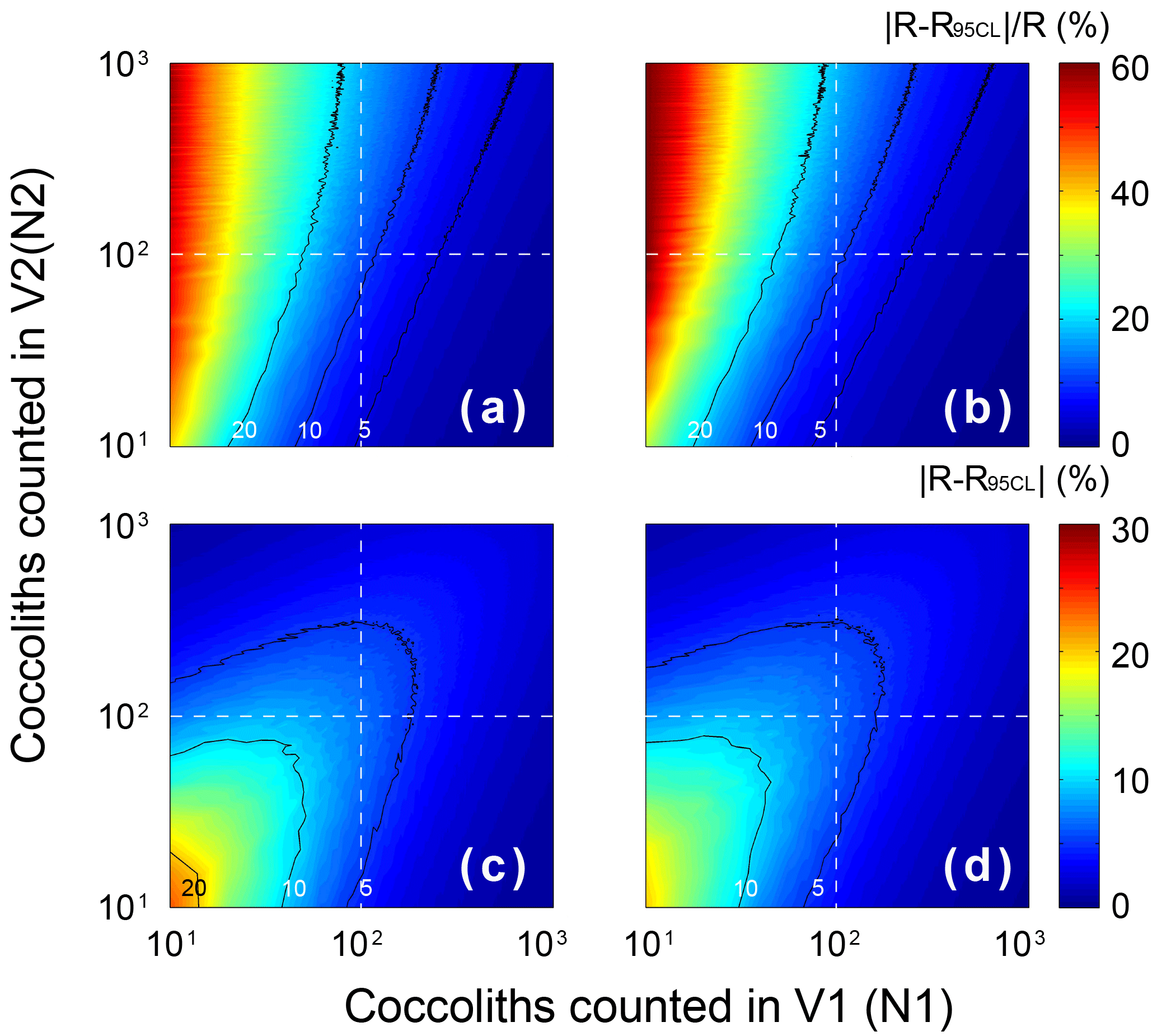
https://www.biogeosciences.net/15/4759/2018/bg-15-4759-2018-f13

Figure E1The error distribution with different N₁ andN₂ (ranging from 1 to 1000) simulated 5000 times by Matlab with assumptions that the error distributions of N₁ and N₂ follow the Poisson distribution. The calculation of R follows Eq. (2)–(5), and here we assume that the numbers of FOV are equal (n₁=n₂). Counter lines mark values equal to 5, 10 and 20. Panels (a) and (c) represent the lower 95 % confidence level, and (b) and (d) represent upper 95 % confidence level. Panels (a) and (b) show the relative error of R, and (c) and (d) represent the absolute error of R.

Download

Author contributions

This study was conceived by HZ and CL. Measurements and calculations were conducted by HZ. HZ, HS and CB wrote the paper with the help from XJ and CL.

Competing interests

The authors declare that they have no conflict of interest.

Acknowledgements

This study was supported by grants from the Chinese National Science Foundation (91428310, 91428309 and 41530964, to Chuanlian Liu) and ETH Zurich (to Heather Stoll). It was also supported by Chinese Scholarship Council (CSC) scholarship to Hongrui Zhang. We thank the Integrated Ocean Drilling Program (IODP) for providing the samples. The IODP is sponsored by the US National Science Foundation and participating countries under management of IODP Management International, Inc (IODP-MI). We thank Zhimin Jian for providing the sample of the core ODP 807. We thank three anonymous reviewers as well as the editor for their comments and suggestions, which helped us to improve the original version of the paper.

Edited by: Lennart de Nooijer
Reviewed by: three anonymous referees

References

Bach, L. T., Riebesell, U., Sett, S., Febiri, S., Rzepka, P., and Schulz, K. G.: An approach for particle sinking velocity measurements in the 3–400 µm size range and considerations on the effect of temperature on sinking rates, Mar. Biol., 159, 1853–1864, https://doi.org/10.1007/s00227-012-1945-2, 2012.

Barnea, E. and Mizrahi, J.: A generalized approach to the fluid dynamics of particulate systems: Part 1. General correlation for fluidization and sedimentation in solid multiparticle systems, Chem. Eng. J., 5, 171–189, https://doi.org/10.1016/0300-9467(73)80008-5, 1973.

Baumann, K.-H.: Importance of size measurements for coccolith carbonate flux estimates, Micropaleontology, 50, 35–43, 2004.

Beaufort, L., Lancelot, Y., Camberlin, P., Cayre, O., Vincent, E., Bassinot, F., and Labeyrie, L.: Insolation cycles as a major control of equatorial Indian Ocean primary production, Science, 278, 1451–1454, https://doi.org/10.1126/science.278.5342.1451, 1997.

Beltran, C., de Rafélis, M., Minoletti, F., Renard, M., Sicre, M. A., and Ezat, U.: Coccolith δ¹⁸O and alkenone records in middle Pliocene orbitally controlled deposits: High-frequency temperature and salinity variations of sea surface water, Geochem. Geophy. Geosy., 8, Q05003, https://doi.org/10.1029/2006GC001483, 2007.

Bolton, C. T. and Stoll, H. M.: Late Miocene threshold response of marine algae to carbon dioxide limitatio, Nature, 500, 558–562, https://doi.org/10.1038/nature12448, 2013.

Bolton, C. T., Stoll, H. M., and Mendez-Vicente, A.: Vital effects in coccolith calcite: Cenozoic climate-pCO₂ drove the diversity of carbon acquisition strategies in coccolithophores, Paleoceanography, 27, PA4204, https://doi.org/10.1029/2012pa002339, 2012.

Bolton, C. T., Hernandez-Sanchez, M. T., Fuertes, M. A., Gonzalez-Lemos, S., Abrevaya, L., Mendez-Vicente, A., Flores, J. A., Probert, I., Giosan, L., Johnson, J., and Stoll, H. M.: Decrease in coccolithophore calcification and CO₂ since the middle Miocene, Nat. Commun., 7, 10284, https://doi.org/10.1038/ncomms10284, 2016.

Bordiga, M., Bartol, M., and Henderiks, J.: Absolute nannofossil abundance estimates: Quantifying the pros and cons of different techniques, Revue de Micropaléontologie, 58, 155–165 https://doi.org/10.1016/j.revmic.2015.05.002, 2015.

Candelier, Y., Minoletti, F., Probert, I., and Hermoso, M.: Temperature dependence of oxygen isotope fractionation in coccolith calcite: A culture and core top calibration of the genus Calcidiscus, Geochim. Cosmochim. Ac., 100, 264–281, https://doi.org/10.1016/j.gca.2012.09.040, 2013.

Channell, J., Sato, T., Kanamatsu, T., Stein, R., and Alvarez Zarikian, C.: Expedition 303/306 synthesis: North Atlantic climate, Channell, JET, edited by: Kanamatsu, T., Sato, T., Stein, R., Alvarez Zarikian, C. A., Malone, M. J., and the Expedition, 303, 306: 4–6, 2010.

Edwards, A. R.: A preparation technique for calcareous nannoplankton, Micropaleontology, 9, 103–104, 1963.

Hammer, Ø., Harper, D., and Ryan, P.: Paleontological Statistics Software: Package for Education and Data Analysis, Palaeontol. Electron., 4, 1–9, 2001.

Hermoso, M., Candelier, Y., Browning, T. J., and Minoletti, F.: Environmental control of the isotopic composition of subfossil coccolith calcite: Are laboratory culture data transferable to the natural environment?, Geoci. Res. J., 7, 35–42, https://doi.org/10.1016/j.grj.2015.05.002, 2015.

Hermoso, M., Chan, I. Z. X., McClelland, H. L. O., Heureux, A. M. C., and Rickaby, R. E. M.: Vanishing coccolith vital effects with alleviated carbon limitation, Biogeosciences, 13, 301–312, https://doi.org/10.5194/bg-13-301-2016, 2016.

Jin, H., Jian, Z., Cheng, X., and Guo, J.: Early Pleistocene formation of the asymmetric east-west pattern of upper water structure in the equatorial Pacific Ocean, Chinese Sci. Bull., 56, 2251–2257, 2011.

Jin, X., Liu, C., Poulton, A. J., Dai, M., and Guo, X.: Coccolithophore responses to environmental variability in the South China Sea: species composition and calcite content, Biogeosciences, 13, 4843–4861, https://doi.org/10.5194/bg-13-4843-2016, 2016.

Kell, G. S.: Density, thermal expansivity, and compressibility of liquid water from 0^∘ to 150^∘ correlations and tables for atmospheric pressure and saturation reviewed and expressed on 1968 temperature scale, J. Chem. Engin. Data, 20, 97–105, 1975.

Kestin, J., Sokolov, M., and Wakeham, W. A.: Viscosity of liquid water in the range −8 ^∘C to 150 ^∘C, J. Phys. Chem. Ref. Data, 7, 941–948, 1978.

Koch, C. and Young, J.: A simple weighing and dilution technique for determining absolute abundances of coccoliths from sediment samples, J. Nannoplankton Res., 29, 67–69, 2007.

Li, C.-F., Lin, J., and Kulhanek, D. K.: South China Sea tectonics: Opening of the South China Sea and its implications for southeastAsian tectonics, climates, and deep mantle processes since the late Mesozoic, IODP Sci. Prosp., 349, 32–39, 2013.

Liang, D. and Liu, C.: Variations and controlling factors of the coccolith weight in the Western Pacific Warm Pool over the last 200 ka, J. Ocean U. China, 15, 456–464, 2016.

McClelland, H. L., Bruggeman, J., Hermoso, M., and Rickaby, R. E.: The origin of carbon isotope vital effects in coccolith calcite, Nat. Commun., 8, 14511, https://doi.org/10.1038/ncomms14511, 2017.

McNown, J. S. and Jamil, M.: Effects of particle shape on settling velocity at low Reynolds numbers, Eos, 31, 74–82, 1950.

Miklasz, K. A. and Denny, M. W.: Diatom sinkings speeds: Improved predictions and insight from a modified Stokes' law, Limnol. Oceanogr., 55, 2513–2525, https://doi.org/10.4319/lo.2010.55.6.2513, 2010.

Minoletti, F., Hermoso, M., and Gressier, V.: Separation of sedimentary micron-sized particles for palaeoceanography and calcareous nannoplankton biogeochemistry, Nat. Protocol., 4, 14–24, https://doi.org/10.1038/nprot.2008.200, 2009.

Paull, C. K. and Thierstein, H. R.: Stable isotopic fractionation among particles in Quaternary coccolith-sized deep-sea sediments, Paleoceanography, 2, 423–429, https://doi.org/10.1029/PA002i004p00423, 1987.

Richardson, J. and Zaki, W.: The sedimentation of a suspension of uniform spheres under conditions of viscous flow, Chem. Eng. Sci., 3, 65–73, 1954.

Rickaby, R. E. M., Henderiks, J., and Young, J. N.: Perturbing phytoplankton: response and isotopic fractionation with changing carbonate chemistry in two coccolithophore species, Clim. Past, 6, 771–785, https://doi.org/10.5194/cp-6-771-2010, 2010.

Rousselle, G., Beltran, C., Sicre, M.-A., Raffi, I., and De Rafélis, M.: Changes in sea-surface conditions in the Equatorial Pacific during the middle Miocene–Pliocene as inferred from coccolith geochemistry, Earth Planet. Sc. Lett., 361, 412–421, https://doi.org/10.1016/j.epsl.2012.11.003, 2013.

Sprengel, C., Baumann, K.-H., Henderiks, J., Henrich, R., and Neuer, S.: Modern coccolithophore and carbonate sedimentation along a productivity gradient in the Canary Islands region: seasonal export production and surface accumulation rates, Deep-Sea Res. Pt. II, 49, 3577–3598 https://doi.org/10.1016/S0967-0645(02)00099-1, 2002.

Stoll, H. M.: Limited range of interspecific vital effects in coccolith stable isotopic records during the Paleocene-Eocene thermal maximum, Paleoceanography, 20, PA1007, https://doi.org/10.1029/2004pa001046, 2005.

Stoll, H. M. and Ziveri, P.: Separation of monospecific and restricted coccolith assemblages from sediments using differential settling velocity, Mar. Micropaleontol., 46, 209–221, https://doi.org/10.1016/S0377-8398(02)00040-3, 2002.

Stoll, H. M., Rosenthal, Y., and Falkowski, P.: Climate proxies from Sr/Ca of coccolith calcite: calibrations from continuous culture of Emiliania huxleyi, Geochim. Cosmochim. Ac., 66, 927–936, https://doi.org/10.1016/S0016-7037(01)00836-5, 2002.

Xie, H.-Y. and Zhang, D.-W.: Stokes shape factor and its application in the measurement of spherity of non-spherical particles, Powder Technol., 114, 102–105, https://doi.org/10.1016/S0032-5910(00)00269-2, 2011.

Young, J. R. and Ziveri, P.: Calculation of coccolith volume and it use in calibration of carbonate flux estimates, Deep-Sea Res. Pt. II, 47, 1679–1700, https://doi.org/10.1016/S0967-0645(00)00003-5, 2000.

Zhang, H., Liu, C., Jin, X., Shi, J., Zhao, S., and Jian, Z.: Dynamics of primary productivity in the northern South China Sea over the past 24,000 years, Geochem. Geophy. Geosy., 17, 4878–4891, https://doi.org/10.1002/2016GC006602, 2016.

Ziveri, P., Stoll, H., Probert, I., Klaas, C., Geisen, M., Ganssen, G., and Young, J.: Stable isotope “vital effects” in coccolith calcite, Earth Planet. Sc. Lett., 210, 137–149, https://doi.org/10.1016/S0012-821X(03)00101-8, 2003.

Articles

Download

Article (31921 KB)
Full-text XML

Short summary

The sinking speeds of coccoliths are relevant for laboratory methods to separate coccoliths for geochemical analysis. However, in the absence of estimates of coccolith settling velocity, previous implementations have depended mainly on time-consuming method development by trial and error. In this study, the sinking velocities of cocooliths were carefully measured for the first time. We also provide an estimation of coccolith sinking velocity by shape, which will make coccolith separation easier.

Technical note: A refinement of coccolith separation methods: measuring the sinking characteristics of coccoliths

2.1 Sample selections

2.2 Experiment designs

2.2.1 Sample pretreatments

2.2.2 Measuring the sinking speeds of coccoliths

2.2.3 Detecting the potential influence of vessels

2.2.4 Other factors influencing the sinking velocity

3.1 Influence of vessels

3.2 Sinking velocities at 20 ∘C in 0.2 % ammonia

3.3 Estimating the sinking velocities

3.2 Sinking velocities at 20 ^∘C in 0.2 % ammonia