2.1 Experimental site O₃HP

Experimental data were obtained at the O₃HP site (Oak Observatory at the Observatoire de Haute Provence, 5^∘42^′44${}^{\prime \prime }$ E, 43^∘55^′54${}^{\prime \prime }$ N). This site constitutes part of the French national network SOERE F-ORE-T (System of Observation and Experimentation, in the long term, for Environmental Research) dedicated to investigating the functioning of the forest ecosystem. The O₃HP site (680 m above mean sea level) is located 60 km north of Marseille and consists of a homogeneous 70–100-year-old coppice dominated by Q. pubescens (5 m in height; leaf area index, LAI = 2.2), which accounts for ≈90 % of the biomass and ≈75 % of the trees. A rainout shelter above 300 m² of the canopy dynamically excluded rainfall by deploying automated shutters. This facility facilitated the study of Q. pubescens under natural and amplified drought, henceforth referred to as the ND and AD plot respectively. In the present study, the device was deployed during rain events from the end of May until October 2012 in order to exclude 32 % of the precipitation in the rain exclusion plot. In practice, almost all rainfall in late spring and summer was thus intercepted, increasing the number of dry days (< 1 mm, Polade et al., 2014) by 22. This percentage corresponds with the highest IPCC projections made for the end of the century over the Mediterranean area and accords with the precipitation reduction at O₃HP during the driest years from 1967 to 2000 compared with the average precipitation over this period. Using an ombrothermic diagram (P < 2T, with P= monthly precipitation in mm and T= monthly air temperature in ^∘C), we assessed that the summer 2012 drought period reaches 4.5 months in the AD plot, compared with 3 months in the ND plot. Ambient and soil environmental parameters were continuously monitored using a dense network of sensors (for details see Sect. 2.7). Access to the canopy was at two levels: ≈0.8 and 3.5 m (top canopy branches) above ground level, with the highest level being the one at which we undertook this study. Further description can be found in Santonja et al. (2015).

2.2 Seasonal sampling strategy

Isoprene emission rate measurements were undertaken for at least 1 week per month from June 2012 to June 2013, except for the period from November 2012 until March 2013 when Q. pubescent is fully senescent, with leaves remaining on the tree (marcescent species). This calendar enabled us to capture isoprene emissions during leaf maturity but also during bud break (April 2013) and just before leaf senescence (October 2012). Three trees were studied in each plot along the whole seasonal cycle, with a single branch at the top of the canopy predominantly sampled for each tree. More intensive measurements were carried out in June 2012 (3 weeks) and April 2013 when tree-to-tree and within-canopy variability was assessed. One ND branch was subsequently sampled throughout all intensive campaigns, and the five other ND and AD branches were alternately sampled during 1 to 2 days (Genard-Zielinski et al., 2015). Isoprene samples were collected on cartridges packed with adsorbents, apart from April 2013 when online isoprene measurements were conducted using a PTR-MS (proton-transfer-reaction mass spectrometer) directly connected to the enclosure via a 50 m $\mathrm{1}/{\mathrm{4}}^{\prime \prime }$ PTFE line. When cartridges were used, samples (volume ranging between 0.45 and 0.9 L, depending on the expected emission intensity) were taken from sunrise to sunset, roughly every 2 h. PTR-MS measurements allowed a higher sampling frequency (between 120 and 390 s⁻¹).

Branch enclosures were generally installed on the day before the first emission rate measurement was taken and at least 2 h beforehand in order for the plant to return to normal physiological functioning. Note that although senescence had just begun in October 2012, we did check that the enclosed branches were not senescent during these measurements.

2.3 Branch-scale isoprene emissions and gas exchanges

Sampling was undertaken using two identical dynamic branch enclosures (detailed description in Genard-Zielinski et al., 2015). Briefly, the device consisted of a ≈60 L PTFE (polytetrafluoroethylene) frame closed by a sealed, 50 µm thick PTFE film, to which ambient air was introduced at Q₀ ranging between 11 and 14 L min⁻¹ using a PTFE pump (KNF N 840.1.2 FT.18^®, Germany). Gas flow rates were controlled by mass flow controllers (Bronkhorst) and all tubing lines were made of PTFE. A PTFE propeller ensured the rapid mixing of air inside the chamber. The microclimate (PAR, photosynthetic active radiation; T; relative humidity) inside the chamber was continuously monitored (relative humidity and temperature probe LI-COR 1400–104^®, and quantum sensor LI-COR, PAR-SA 190^®; Lincoln, NE, USA) and recorded (LI-COR 1400^®; Lincoln, NE, USA). CO₂–H₂O exchanges from the enclosed branches were also continuously measured using infrared gas analysers (IRGA 840A^®, LI-COR) in order to assess the net assimilation P_n (in µmol${}_{{\mathrm{CO}}_{\mathrm{2}}}$ m⁻² s⁻¹) and the stomatal conductance to water vapour G_w (mol${}_{\mathrm{H}{}_{\mathrm{2}}\mathrm{O}}$ m⁻² s⁻¹) using the equations from Von Caemmerer and Farquhar (1981) as detailed in Genard-Zielinski et al. (2015).

Total dry biomass matter (DM) was calculated by manually scanning every leaf of each sampled branch enclosed in the chamber and applying a dry leaf mass per area conversion factor (LMA) extrapolated from concomitant measurements made on the same site. The mean (range) DM was 0.16 (0.01–0.45) g_DM, and mean (range) LMA was 13.17 (0.82–36.67) g_DM cm⁻².

Isoprene emission rates (ER) were calculated as

where ER is expressed in µgC g${}_{\mathrm{DM}}^{-\mathrm{1}}$ h⁻¹, Q₀ is the flow rate of the air introduced into the chamber (L h⁻¹), C_in and C_out are the concentrations in the inflowing and outflowing air (µgC L⁻¹), and DM is the sampled dry biomass matter (g_DM).

Throughout the seasonal cycle, except in April, isoprene was collected using packed cartridges (glass and stainless-steel) prefilled with Tenax TA and/or Carbotrap. Isoprene was then analysed in the laboratory according to a gas chromatography–mass spectrometry (GM-MS) procedure detailed in Genard-Zielinski et al. (2015), with a level of analytical precision greater than 7.5 %.

In April 2013, two types of PTR-MS were used for online isoprene sampling and analysis. A quadrupole PTR-MS (HS-PTR-MS, Ionicon Analytik GmbH, Innsbruck Austria), connected to the ND branch enclosure, was operated at 2.2 mbar pressure, 60 ^∘C temperature, and 500 V voltage in order to achieve an E∕N ratio of ≈115 Td (E: electric field strength (V cm⁻¹); N: buffer gas number density (molecule cm⁻³); 1 Td = 10⁻¹⁷ V cm²). The primary H₃O⁺ ion count assessed at m∕z 21 was 3×10⁷ cps, with a typically < 10 % contribution monitored from the first water cluster (m∕z 37) and < 5 % contribution from the ${\mathrm{O}}_{\mathrm{2}}^{+}$ (m∕z 32). Measurements were operated in scan mode (m∕z 21 to m∕z 210) every 380 s. After 15–20 min of sampling of incoming air, the outgoing air was sampled for 30 to 60 min. A high-resolution ($m/\mathrm{\Delta }m\approx \mathrm{4000}$) time-of-flight PTR-MS (PTR-ToF-MS-8000, Ionicon Analytik GmbH, Innsbruck Austria) connected to the second enclosure used in our study enabled us to discriminate between compounds when their masses differ at the tenth part. The main experimental characteristics were similar to the HS-PTR-MS, but a voltage of 550 V was used in order to reach an E∕N ratio of ≈125 Td. The H₃O⁺ ion count assessed at m∕z 21 was 1.1×10⁶ cps with a similar < 10 % contribution monitored from the first water cluster (m∕z 37) and < 2.5 % contribution from the ${\mathrm{O}}_{\mathrm{2}}^{+}$ (m∕z 32). The signal at m∕z 69 corresponding to protonated isoprene was converted into mixing ratio by using a proton transfer rate constant k of $\mathrm{1.96}\times {\mathrm{10}}^{-\mathrm{9}}$ cm³ s⁻¹ (Cappellin et al., 2012), the reaction time in the drift tube, and the experimentally determined ion transmission efficiency. The relative ion transmission efficiencies of both instruments were assessed using a standard gas calibration mixture (TO-14A Aromatic Mix, Restek Corporation, Bellefonte, USA; 100±10 ppb in nitrogen). Assuming an uncertainty of ±15 % in the k-rate constants and in the mass transmission efficiency, the overall uncertainty of the concentration measurement is estimated to be of the order of ±20 %. Background signal was obtained by passing air through a platinum catalytic converter heated at 300 ^∘C. Detection limits defined as 3 times the standard deviation on the background signal were 10 and 50 ppt with the PTR-ToF-MS and the HS-PTR-MS respectively. An intercomparison between both the cartridge + GC-MS and PTR-MS protocols was undertaken parallel to another emitter present on the site (Acer monspessulanum); no significant difference was observed between the techniques (Genard-Zielinski et al., 2015).

The overall uncertainty (sampling + analysis) on ER assessment was between 20 % and 25 %.

2.4 Statistics

All statistics were performed on STATGRAPHICS^® centurion XV by Statpoint, Inc. Differences in P_n, G_w, ER, and Q. pubescens isoprene emission factors (ε_iso,Qp, see Sect. 2.5 for details) between the ND and the AD plot were tested using Mann–Whitney U tests. Seasonal changes in these ecophysiological parameters were tested using the Kruskal–Wallis test and the analysis was performed separately on trees from the ND and AD plot. Comparisons between COOPERATE environmental data (see Sect. 2.7) were made using a Wilcoxon test when data were not log-normal and a t test when log-normal.

2.5 Branch-scale ER assessment using MEGAN2.1 emission model

Based on the latest version of the MEGAN model (MEGAN2.1, Guenther et al., 2012), Q. pubescens ER were assessed for the sampling conditions of our seasonal study using

Nota bene: in order to be comparable with our measurements carried out on top canopy leaves and expressed as net emission rates in the unit of µgC g${}_{\mathrm{DM}}^{-\mathrm{1}}$ h⁻¹, no canopy environment coefficient C_CE nor LAI was considered in the calculation of γ_iso and thus in ER_MEGAN (for further details see Guenther et al., 2012).

2.6 Branch-scale ER assessment using an artificial neural network trained on field data

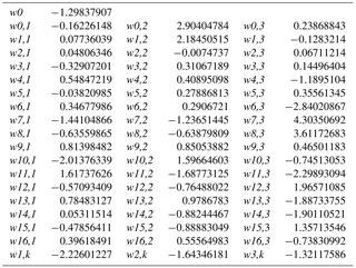
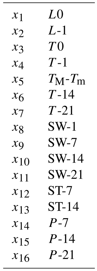
The artificial neural network (ANN) developed in this study to assess branch-scale ER from Q. pubescens (henceforth referred to as G14) was based on a commercial version of the Netral NeuroOne software v.6.0 (http://www.inmodelia.com/, France; last access: 31 July 2018). The ANN was used as a multilayer perceptron (MLP) in order to calculate multiple non-linear regressions between a set of input regressors x_i (the environmental variables measured at the O₃HP) and the output data (the measured isoprene ER). The assessed ER (ER_G14) was calculated as follows:

where w₀ is the connecting weight between the bias and the output, N the number of neurons N_j, f the transfer function, w_0,j the connecting weight between the bias and the neuron N_j, w_i the connecting weight between the input and the neuron N_j, and x_i the n input regressors. The MLP optimisation of the weights w was achieved according to Boissard et al. (2008). Every input regressor x_i was centrally normalised. Two sub-datasets were considered, for the ND and AD plot respectively. For each sub-dataset, 80 % of our data were used for training and optimising the MLP, and the remaining 20 % were used for blind validation based on root mean square error (RMSE). Training–validation splitting was made using a Kullback–Leibler distance function available in NeuroOne v 6.0. Only the non-linear hyperbolic tangent (tanh) function was tested as transfer function f. Up to N=7 neurons (distributed in only one layer) were tested for every ANN setting. The overtraining phenomenon (a too-large number of neurons vs. the number of input parameters) was checked against the RMSE_training∕ RMSE_validation evolution vs. the number N of neurons tested: training was stopped for RMSE_training > RMSE_validation when N≥3.

Among the other available statistical methods, ANNs present the advantage of being the most parsimonious, i.e., giving the smallest error for a same number of descriptors (see for instance Dreyfus et al., 2002). Moreover, the ANN approach, as is the case of other non-linear regression methods, is not particularly sensitive to regressors' co-linearity (Bishop, 1995; Dreyfus et al., 2002). On the other hand, one of the limitations of ANNs is that they can only be employed for interpolation within the range of values of the trained data, and not for extrapolation exercises beyond this range. Consequently, during the isoprene emission sensitivity to future climatic changes (see Sect. 2.8), only x_i values fitting within the range of variation (±20 %) tested during the training phase were considered; in total 21 % of the data were thus rejected.

2.7 COOPERATE environmental database

Ambient and edaphic parameters used for the ANN optimisation were obtained from the COOPERATE database (https://cooperate.obs-hp.fr/db, last access: 31 July 2018) and daily averaged for each day of our study. Ambient PAR (µmol m⁻² s⁻¹) measured above the canopy at 6.5 m (LI-COR Li-190^®; Lincoln, NE, USA) in the ND plot was used as the PAR reaching all of the top canopy branches studied. Ambient air temperature (T, ^∘C) measured at 6.15 m (CS215, Campbell Scientific Ltd., UK) in the ND and AD plot was used for both sets of branches. Since some precipitation (P, mm) values were missing (< 5 %) from the COOPERATE database during our data processing, P values from the nearby (< 10 km) Forcalquier meteorological station were used. The bias between cumulated P (P_cum) curves at both sites was assessed and considered in order to extrapolate the missing values at the O₃HP site. As P was cumulated over 7, 14, and 21 days, the resulting bias was negligible (≈ 1 %) and no further adjustment was made. Soil water content (SW, L L⁻¹) and temperature (ST, ^∘C) at −0.1 m (Hydra Probe II, Stevens, Water Monitoring Systems Inc., OR, USA) specific to each of the sampled trees were selected and extracted from the COOPERATE database; when soil data were missing, they were extrapolated from the nearest equivalent data point measurement. Daily mean PAR, T, P, SW, and ST were cumulated over a time period ranging from 1 to 21 days before the measurement.

2.8 ORCHIDEE land surface model: providing future conditions to investigate ER sensitivity to climatic changes

Present-day T and P were assessed as the 2000–2010 daily averages derived from the ISI-MIP (Inter-Sectoral Impact Model Intercomparison Project) climate dataset (Warszawski et al., 2014) over the Mediterranean area. This dataset contains the bias-corrected daily simulation outputs of the Earth system model HadGEM2-ES. Corresponding values for the 2090–2100 period were used to assess the expected range of future climatic changes. They were derived from two ISI-MIP future projections forced along two representative concentration pathways (RCPs): the so-called “peak-and-decline” greenhouse gas concentration scenario RCP2.6 (optimistic or moderate scenario) and the “rising” greenhouse gas concentration scenario RCP8.5 (extreme or severe scenario). All T and P data were extracted for the entire Mediterranean region from the global ISI-MIP dataset and subsequently averaged over the area.

Using these present and future T, P, and PAR values (ISI-MIP derived), the corresponding present and future SW and ST were assessed by running the global land surface model ORCHIDEE (ORganising Carbon and Hydrology In Dynamic EcosystEms) over the European part of the Mediterranean region. The calculated SW and ST were averaged over this area. ORCHIDEE is a spatially explicit, process-based model that calculates the CO₂, H₂O, and heat fluxes between the land surface and the atmosphere. Vegetation species distributed at the Earth's surface are represented in ORCHIDEE through 13 plant functional types (PFTs). Processes in the model are represented at the time step of 0.5 h, but the variations of water and carbon pools are calculated on a daily basis. A detailed description of ORCHIDEE is provided by Krinner et al. (2005). Simulations over the European part of the Mediterranean region were performed with the ORCHIDEE model at 0.5×0.5^∘ spatial resolution using the soil parameters (clay, silt, and sand fractions) from Zobler (1986). Given that this study focuses on isoprene emissions from Q. pubescens, we fixed the vegetation with the corresponding PFT “temperate broad-leaf summer green tree”. The described ISI-MIP historical forcings and the ISI-MIP future projections were used as climate conditions for ORCHIDEE runs and ER assessment using G14. Equilibrium was reached by running ORCHIDEE on the first decade of the climate forcing (1961–1990) repeated in a loop and the value of atmospheric CO₂ corresponding to the year 1961. Among the two different hydrology schemes available in ORCHIDEE, the physically based 11-layer scheme was used (Guimberteau et al., 2013).

ER sensitivity to moderate and severe temperature and/or precipitation changes was evaluated using G14 under 6 cases: (i) the T (respectively P) test was conducted considering only T and ST (respectively only P and SW) changes according to the RCP2.6 scenario; (ii) the TT and PP tests were similar to the T and P tests but considered changes according to the RCP8.5 scenario; (iii) the T+P (respectively TT+PP) test combined the effect of T, ST, P, and SW changes according to RCP2.6 (respectively RCP8.5).

3.1 Environmental conditions observed at the O₃HP

Mean daily ambient air temperature T varied between −3 and 26 ^∘C (January 2013 and August 2012 respectively, Fig. 1a). Seasonal PAR variations were in line with T variations, with the daily mean peaking at 900 µmol m⁻² s⁻¹ in July (Fig. 1b). In 2012, the amplification of the ND was adjusted from May to reach its maximum (32 %) in July and maintained until November when rain exclusion was stopped (Fig. 1c). The annual P_cum in the AD plot was lower by 273 mm than in the ND plot at the end of 2012 (782 compared to 509 mm). In 2013 the AD started only at the end of June, simulating a later amplification. From August until October 2012, SW was 50 %–90 % lower in the AD plot than in the ND plot (≈0.02 and to 0.05 L${}_{\mathrm{H}{}_{\mathrm{2}}\mathrm{O}}$ L${}_{\mathrm{soil}}^{-\mathrm{1}}$ respectively in August, Fig. 1d). The AD plot soil water deficit remained significant until the end of the experiment (Mann–Whitney, P < 0.05 in June 2012, P < 0.001 from July 2012 to June 2013), although the rain exclusion system was not activated between December 2012 and June 2013.

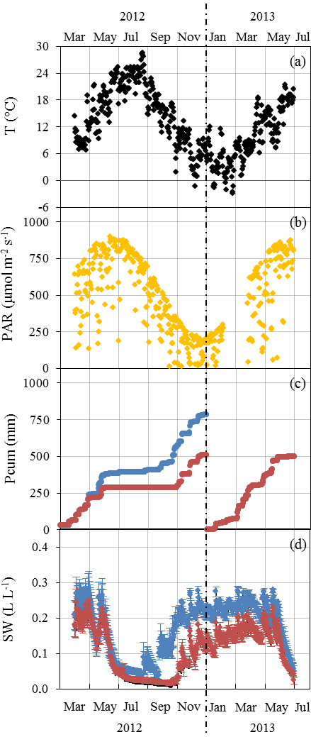
Figure 1Seasonal variations of daily environmental parameters measured at the O₃HP from March 2012 to June 2013. (a) Ambient air temperature T was obtained at 6.5 m above ground level (a.g.l.), approximatively 1.5 m above the canopy. (b) Photosynthetic active radiations PAR received at 6.5 m a.g.l. in the ND plot. (c) Cumulated precipitation P_cum measured over the ND (blue) and AD (red) plot. (d) Mean soil water content SW ± SD measured at −0.1 m depth from various soil probes in the ND (blue, n=3) and AD (red, n=5) plot.

Download

No significant difference was noticed for monthly PAR and T means between the ND and the AD plot, except in September 2012 when branches sampled on the ND plot received significantly more PAR than branches on the AD plot (Mann–Whitney, P < 0.001). This difference could be due to an orientation of the branches sampled in the ND plot in September that enabled greater receipt of PAR during our measurements than the AN sampled branches.

3.2 Gas exchange and isoprene seasonal variations

G_w and P_n showed similar seasonal patterns in both plots (Fig. 2a, b), with the lowest values in July–September (10–20 mol${}_{\mathrm{H}{}_{\mathrm{2}}\mathrm{O}}$ m⁻² s⁻¹ and ≈1 µmol${}_{{\mathrm{CO}}_{\mathrm{2}}}$ m⁻² s⁻¹ respectively) and the highest in June (80–170 mol${}_{\mathrm{H}{}_{\mathrm{2}}\mathrm{O}}$ m² s⁻¹ and ≈9 µmol${}_{{\mathrm{CO}}_{\mathrm{2}}}$ m⁻² s⁻¹ respectively). Respiration dominated over gross CO₂ assimilation in April, resulting in negative net assimilation ($P_{\mathrm{n}}\approx -\mathrm{1}$ µmol${}_{{\mathrm{CO}}_{\mathrm{2}}}$ m⁻² s⁻¹) in both plots. In contrast, G_w and P_n were not influenced by water stress in the same way. Whereas G_w was significantly reduced under AD from July 2012, P_n remained stable, except in June 2013 when P_n values that were twice as high under AD than ND were observed. It is important to note that the tomography measurements made at this site showed that oak roots were predominantly distributed in the outermost humiferous horizon located above a calcareous slab at a 10–20 cm depth and that only very few roots crossed this slab.

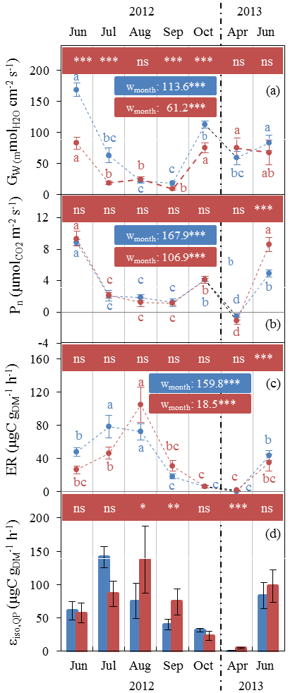
Figure 2Seasonal variations of monthly Q. pubescens gas exchanges observed at O₃HP (June 2012 to June 2013) under ND (blue) and AD (red) (mean ± SD). (a) Stomatal conductance to water vapour G_w. (b) Net photosynthetic assimilation P_n. (c) Measured branch isoprene emission rate ER. (d) Isoprene emission factor (I_s) calculated according to Guenther et al. (1995) using in situ ER vs. C_L×C_T correlations, except in July where mean ER measured under enclosure conditions close to 1000 µmol m⁻² s⁻¹ and 30 ^∘C was used. Differences between ND and AD using Mann–Whitney U tests are denoted using lower case letters (a > b > c > d). Differences among water treatment stress using Kruskal–Wallis tests are denoted by asterisks (*: P < 0.05; **: P < 0.01; ***: P < 0.001).

Download

Water stress only affected the ER seasonal pattern during summer (Fig. 2c). Maximum ER was delayed by a month in the AD plot (104.8 µgC g${}_{\mathrm{DM}}^{-\mathrm{1}}$ h⁻¹ in August) in comparison to the ND plot (78.5 µgC g${}_{\mathrm{DM}}^{-\mathrm{1}}$ h⁻¹ in July). ER was lowest in October (≈6 µgC g${}_{\mathrm{DM}}^{-\mathrm{1}}$ h⁻¹ in both plots). During April bud break and isoprene emission onset, ER was as low as 0.5 and 1 µgC g${}_{\mathrm{DM}}^{-\mathrm{1}}$ h⁻¹ in the ND and AD plot respectively.

Figure 3Comparison between isoprene emission rates (in µgC g${}_{\mathrm{DM}}^{-\mathrm{1}}$ h⁻¹) calculated using MEGAN2.1 (ER_MEGAN, Guenther et al., 2012) and measured isoprene emission rates (ER) vs. the wilting point value θw (0.005 to 0.15 m³ m⁻³), from June 2012 to June 2013, under (a) ND (n=267) and (b) AD (n=138). Since the rain exclusion device was only implemented soon prior to our study's commencement in June 2012, the ND and AD measurements were considered together for June 2012. Linear regressions for ND June 2012 were $y=\mathrm{1.13}x-\mathrm{12.05}$, R²=0.80 (θw= 0.05 m³ m⁻³); $y=\mathrm{1.13}x-\mathrm{7.13}$, R²=0.80 (θw=0.1 m³ m⁻³); and $y=\mathrm{1.12}x-\mathrm{16.94}$, R²=0.76 (θw= 0.15 m³ m⁻³). The dotted line is the 1:1 line.

Download

Although ε_iso,Qp was calculated every month as the slope of ER vs. C_L×C_T (as in Guenther et al., 1995), this correlation was not significant in July, especially in the case of AD branches (P > 0.05, R²=0.06 and 0.01 for ND and AD respectively). As a result, ε_iso,Qp in July was calculated by averaging ER measured under environmental conditions close to 1000±100 µmol m⁻² s⁻¹ and 30±1 ^∘C. In general, AD branches showed poorer ER vs. C_L×C_T correlations than branches growing in the ND plot (data not shown). ε_iso,Qp was significantly higher by a factor of 2 in August and September for the AD branches compared to the ND (Fig. 2d). As for ER, ε_iso,Qp maximum was reached in August (137.8 µgC g${}_{\mathrm{DM}}^{-\mathrm{1}}$ h⁻¹) in the AD plot, while the maximum in the ND plot occurred in July (74.3 µgC g${}_{\mathrm{DM}}^{-\mathrm{1}}$ h⁻¹). The general high variability observed in April during the isoprene emission onset (some branches were already emitting, while some were not yet emitting isoprene, regardless of their locations in the AD ∕ ND plots) was as large as the AD–ND variability and thus could not solely be attributed to the water stress treatment. The relative annual ε_iso,Qp difference between ND and AD was +45 %.

3.3 Modelling the isoprene seasonal variations of Q. pubescens at the O₃HP

Given that we were aiming to test the capacity of an empirically based isoprene emission model to describe seasonal ER variability and sensitivity to drought observed during this study, we tested the latest version of the MEGAN model, which is widely used for air quality and climate change applications (MEGAN2.1, Guenther et al., 2012). In particular, the ability of its soil moisture coefficient activity γ_SM (Eq. 4a–c) to assess the observed effect of ND and AD treatments was examined over wilting point θ_w values ranging from 0.01 to 0.15 m³ m⁻³, which is representative of a large brand of soils (Ghanbarian-Alavijeh and Millàn, 2009). Indeed, Müller et al. (2008) showed that isoprene assessments were very sensitive to θ_w. For the record, θ_w was 0.15 m³ m⁻³ at the O₃HP.

Assessed (ER_MEGAN) and observed (ER) isoprene emission rates were compared separately for ND and AD. However, given that the rainout shelter was implemented close to the commencement of our study in June 2012, measurements carried out in the AD plot were not distinguished, only in the case of this month, from the ones taken in the ND plot (AD and ND data were thus mixed for June 2012).

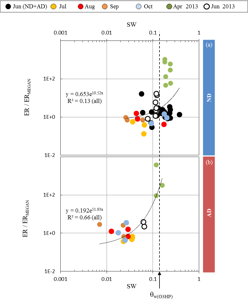
Figure 4Ratio between observed (ER) and calculated (ER_MEGAN) isoprene emission rates vs. the soil water content SW measured at the O₃HP, under (a) ND (n=267) and (b) AD (n=138). Given that the rain exclusion device was only implemented just before our study began in June 2012, the ND and AD measurements were considered together for June 2012. The dotted line is for SW =θw measured at O₃HP (0.15 m³ m⁻³).

Download

For θ_w< 0.05 m³ m⁻³, and regardless of the θ_w value, MEGAN2.1 captured more than 80 % of the ER variability in the ND plot ($y=\mathrm{0.15}{x}^{\mathrm{1},\mathrm{5}}$, R²=0.81, Fig. 3a), but less (≈ 50 %) in the AD plot (R²=0.53 and 0.54 for θ_w= 0.005 and 0.01 m³ m⁻³ respectively, Fig. 3b). An overall over-estimation of 25 % was associated with the MEGAN2.1 assessment for both treatments. On the contrary, for θ_w≥0.05 m³ m⁻³, most of the isoprene emissions were set to zero by MEGAN2.1 in the AD plot, while in the ND only June observations were correctly assessed with an overall over-estimation (regardless of the θ_w values) of ≈10 % (R² ranging from 0.76 to 0.80 for θ_w= 0.15 and 0.1 m³ m⁻³ respectively). If some of the July ER_MEGAN were fairly close to the observations for θ_w= 0.1 m³ m⁻³, the overall correlation was poor ($y=\mathrm{0.2}x+\mathrm{49.5}$, R²=002).

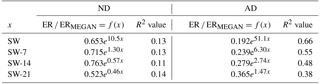
Assuming that the discrepancies between ER_MEGAN and ER only resulted from the γ_SM formulation in MEGAN2.1 (and not from the other activity coefficients γ_P, γ_T, or γ_A used, Eq. 3), ER ∕ ER_MEGAN was calculated for both ND and AD treatments and was considered against the measured SW. In the ND treatment, ER ∕ ER_MEGAN was not found to be significantly dependent on SW (y=0.653e^10.52x, R²=0.13, Fig. 4a). However, in the AD plot, ER ∕ ER_MEGAN increased exponentially with SW (y=0.192e^51.93x, R²=0.66, Fig. 4b) and in particular when SW became higher than the wilting point θ_w measured at the O₃HP site (0.15 m³ m⁻³). Similar findings were obtained for SW-7, SW-14 and SW-21, for both the ND and AD treatments (Table 1).

In order to provide a better description of the impacts of ND and AD on ER as observed at the O₃HP, an empirical type model, based on ANN optimisation of our observations at the O₃HP, was developed specifically for Q. pubescens isoprene emissions. Training and validation of the different ANNs tested were made using values of ER, T, P, PAR, ST, and SW measured at the O₃HP (COOPERATE database). Environmental regressors x_i were integrated, using daily means, over a period ranging from 0 to 21 days prior to the measurements.

Table 1Correlations between ER_MEGAN∕ ER and the soil water content (SW) cumulated over 7 to 21 days before the measurement. ER_MEGAN and ER are isoprene emission rates calculated using MEGAN2.1 (Guenther et al., 2012) and measured (this study) respectively.

Download Print Version | Download XLSX

Among the different ANN settings tested, an optimised architecture, G14 (lowest RMSE between calculated and measured values, no overtraining, best correlation between measured and calculated ER over the whole range of value, see Boissard et al., 2008), was found for N=3 and a set of 16 x_i with their corresponding connecting weights w_i (Appendix A). The final optimised RMSE (validation data) was 8.5 µgC g${}_{\mathrm{DM}}^{-\mathrm{1}}$ h⁻¹, for ER values ranging from 0.06 to 113 µgC g${}_{\mathrm{DM}}^{-\mathrm{1}}$ h⁻¹, and represents 35 % of the mean (22.7 µgC g${}_{\mathrm{DM}}^{-\mathrm{1}}$ h⁻¹). More than 80 % of the ER seasonal variations were assessed by G14, regardless of the water treatment (ND or AD) and the month, except in July (Fig. 5a), when ER variability was always poorly represented regardless of the different ANN settings considered. July corresponds to the period where trees started to adapt to ND and AD; this period was possibly insufficiently represented in our dataset to be well taken into account by our statistical approach. An overall underestimation of 6 % and 12 % was observed in the ND and AD respectively. For comparison, ER_MEGAN calculated with a value θ_w of 0.15 m³ m⁻³ are presented again in Fig. 5b for both the ND and AD treatment.

Figure 5Calculated vs. measured isoprene emission rates (in µgC g${}_{\mathrm{DM}}^{-\mathrm{1}}$ h⁻¹) under ND (n=267) and AD (n=138) from June 2012 to June 2013, using the (a) G14 (this study) and (b) MEGAN2.1 isoprene model (Guenther et al., 2012) with a wilting point value θw of 0.15 m³ m⁻³ (measured at the O₃HP). The dotted line is the 1:1 line.

Download

Under ND, the global contribution of the two lowest frequencies (−14 and −21 days) considered in G14 was, relative to the contribution of the two highest frequencies (instantaneous and −7 days), higher than under AD (Fig. 6). In particular, in October 2012 and April and June 2013, the two lowest frequencies respectively represented 20 %, 97 %, and 50 % of the total in the ND compared to 3 %, 55 %, and 26 % in the AD.

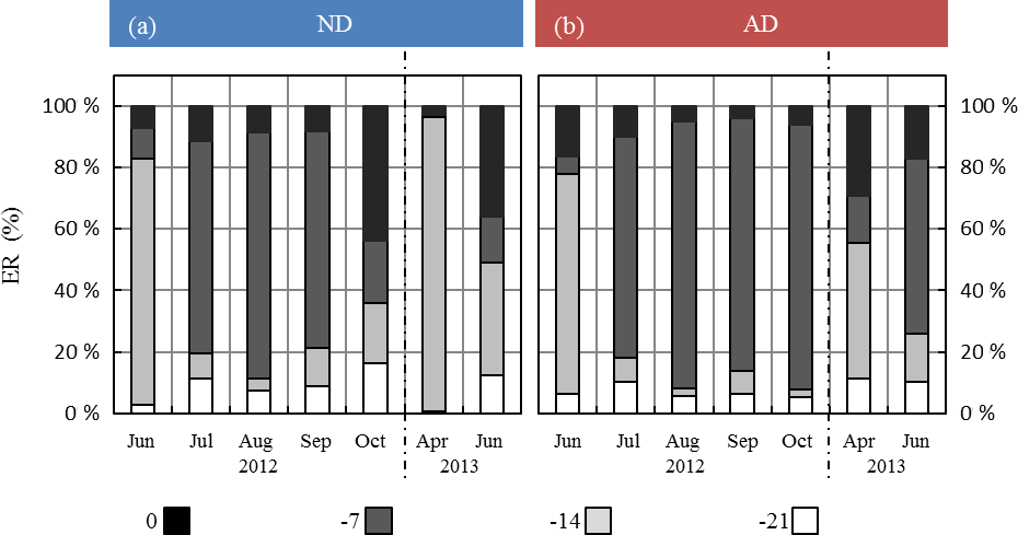
Figure 6Seasonal variations of the relative contribution of the different frequencies as considered in G14 (0, 7, 14, and 21 days before the measurement) among the regressor x_i selected in G14, under (a) ND (n=267) and (b) AD (n=138). The frequency “0”, “−7”, “−14”, “−21” includes the contribution of “L-1, T-1, SW-1, T0, L0, T_M-T_m”; “SW-7, ST-7, P-7”; “T-14, SW-14, ST-14, P-14”; and “T-21, SW-21, P-21” respectively.

Download

3.4 ER sensitivity to expected climatic changes over the European Mediterranean area

Present and future T, P, and PAR (ISI-MIP derived) as well as SW and ST (ORCHIDEE derived) were integrated over periods ranging from 0 to 21 days in order to be used in G14 and to assess ER_G14 for present and future cases. Moderate (respectively severe) changes with regard to the present of SW, P, ST, T, and PAR were additionally calculated according to the RCP2.6 (respectively RCP8.5) scenario; however, PAR relative changes were not considered as they were negligible for both moderate and severe scenarios.

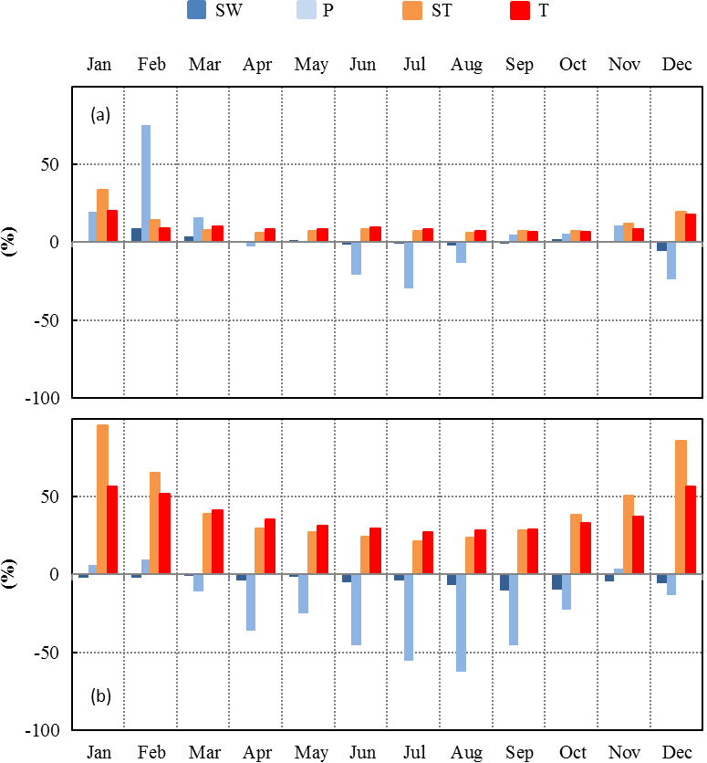
Figure 7Seasonal variations between present (2000–2010) and future (2090–2100) relative changes of SW, P, ST, and T over the continental Mediterranean area obtained using (a) RCP2.6 and (b) RCP8.5 projections.

Download

Table 2Annual absolute and relative changes to the present of SW, P, ST and T according to the RCP2.6 and RCP8.5 scenarios. Present and future cases were calculated for 2000–2010 and 2090–2100 respectively.

Download Print Version | Download XLSX

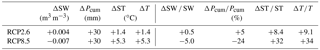
Moderate changes of the environmental conditions (RCP2.6 scenario) implied a systematic positive monthly ΔT throughout the year, whereas ΔP was found to be positive only during the winter and negative during the summer (Fig. 7a). ST and SW changes were found to be in line with T and P respectively. The highest monthly relative changes were for P (+75 % in February and −30 % in July), whereas the smallest were for SW. Monthly ST and T relative changes remained more or less constant (between +7 % and +10 %) between February and November. Overall, T and P_cum absolute (relative) annual changes were +1.4 ^∘C and +34 mm respectively (+9.1 % and +4.8 % respectively, Table 2).

Under more severe environmental changes (RCP8.5 scenario), monthly T and ST increased all year round, whereas P and SW generally decreased, except in January, February, and November, when relative P changes were negligible (Fig. 7b). The annual absolute (relative) changes for T and P_cum were +5.3 ^∘C and −124 mm respectively (+34 % and −24 % respectively, Table 2). In these conditions, the annual ΔP_cum∕P_cum was similar to the reduction experienced at the O₃HP during our study (−30 %). The highest monthly relative changes were found for ST: +96 % and +86 % in January and December respectively. During summertime the highest relative changes were found for P (−55 % and −62 % in July and August respectively).

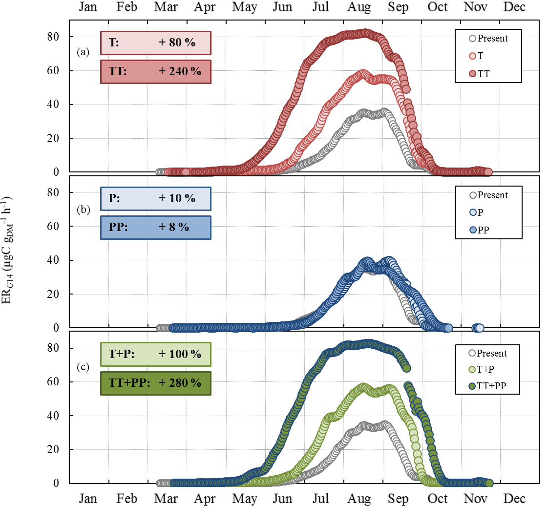
Figure 8Sensitivity of the seasonal variation of isoprene emission rates calculated using G14 (ER_G14, in µgC g${}_{\mathrm{DM}}^{-\mathrm{1}}$ h⁻¹, this study) to (a) T and ST changes as in RCP2.6 (T case) and RCP8.5 (TT case) respectively; (b) SW and P changes as in RCP2.6 (P case) and RCP8.5 (PP case) respectively; and (c) combined T, ST, P, and SW changes as in RCP2.6 (T+P case) and RCP8.5 (TT+PP case) respectively. Present and future cases were calculated for 2000–2010 and 2090–2100 respectively. Overall annual relative changes to present are framed.

Download

ER_G14 was found to systematically increase compared to the present under T and TT changes, with an annual relative change of +80 % and +240 % respectively (Fig. 8a). The highest relative changes were noted in June and July. In contrast, ER_G14 was almost not sensitive to P or PP changes, regardless of the month (annual relative change of +10 % and +8 % respectively, Fig. 8b). When the combined impacts of changes in temperature and precipitation were considered, ER_G14 was found to systemically increase all year round, following a seasonal trend that was extremely close to that found for the T and TT tests (Fig. 8c). However, the additional effect of the precipitation changes enhanced the increase noticed for temperature changes only: the annual increase was +100 % (T+P) and +280 % (TT+PP) compared to +80 % (T) and +240 % (TT). Note that the ER_G14 seasonal trend calculated for the present did not match our observed ER variations. Indeed ER_G14 was tuned using environmental parameters averaged over 24 h (and therefore integrated over the daytime and nighttime period), which were thus much lower than the environmental parameters measured during our daytime-only samplings (especially for PAR and T).

4.1 Impact of water stress on seasonal gas exchanges and isoprene emission of Q. pubescens

In spite of a significant G_w reduction in summer 2012 owing to the AD, Q. pubescens maintained a positive P_n during the summer, regardless of water stress (ND or AD). Electric resistivity tomography measurements carried out on the O₃HP site revealed the heterogeneity of the karstic substrate, organised as soil pockets developed between limestone rocks. Water and nutrient pools and dynamics probably differed greatly between the shallow upper soil layers and the soil pockets developed between limestone rocks. However, the soil trenches in the site revealed that a calcareous slab often developed at a depth of 10–20 cm and that the roots of the oaks were often distributed in this humiferous horizon close to the surface, with very few roots crossing this slab. Water supply from layers deeper than 10–20 cm was thus not considered. Such behaviour enables trees to limit evapotranspiration under water stress, as a drought-acclimated species permits them to ensure sufficient accumulation of carbohydrates for the winter (Chaves et al., 2002). Such a strategy was also observed in a study conducted on the same species but under greenhouse conditions (Genard-Zielinski et al., 2015). The seasonal regulation and conservation of P_n and G_w enabled isoprene emissions to be maintained even during the summer water stress (ND and AD).

The maximum ε_iso,Qp in both plots was close to previously measured values obtained for the same species under Mediterranean conditions during greenhouse and in situ experiments (114.3 and 134.7 µgC g${}_{\mathrm{DM}}^{-\mathrm{1}}$ h⁻¹) by Genard-Zielinski et al. (2015) and Simon et al. (2005) respectively. The difference observed in April 2013 between ε_iso,Qp in the ND and AD could not be attributed solely to the AD effect. Indeed, apart from a possible “memory effect” of the AD applied during 2012, the observed difference was probably due to the high natural variability in bud breaking and isoprene emission onset at this point of the year. The observed significant increase (a factor of 2) in ε_iso,Qp under AD (August and September) illustrates how isoprene is likely to be important for short-term Q. pubescens drought resistance, in particular through the ability of isoprene to stabilise the thylakoids membrane, under (for example) thermal or oxidative stress (Peñuelas et al., 2005; Velikova et al., 2012). Moreover, previous studies have highlighted the possibility for a plant growing under water stress to synthesise isoprene using an alternative carbon source (extra-chloroplastic carbohydrates) (Lichtenthaler et al., 1997; Funk et al., 2004; Brilli et al., 2007). For species emitting other BVOCs than isoprene, but studied in the Mediterranean area under water stress, Lavoir et al. (2009) reported lower (a factor of ≈2) monoterpene emission rates from Quercus ilex under AD from June to August, during the second and third year of rain exclusion. Since Q. ilex does not possess specific leaf reservoirs for monoterpene storage, Q. ilex monoterpene emissions are hence de novo and their emissions are tightly related to their synthesis according to light and temperature as isoprene.

The significant uncoupling between ER and C_L×C_T reported for the July measurements occurred when SW significantly decreased to their seasonal minimum values (0.05 and 0.03 m³ m⁻³) at the O₃HP in both plots. A similar uncoupling has also been observed for some other strong isoprene emitters under water stress (Quercus serrata and Quercus crispula, Tani et al., 2011). These findings may confirm these authors' assumptions that extra-chloroplastic isoprene precursors supply the carbon basis for isoprene biosynthesis (and not only from CO₂ fixed instantaneously in the chloroplast) when water stress occurs, which explains why isoprene emissions become less dependent on the classical abiotic factors PAR and T as considered by Guenther et al. (1995).

4.2 Improving consideration of the drought effect in isoprene emission models

Since ND and AD conditions tested by Q. pubescens in our study stood aside from optimal growth conditions under which empirical emission models perform fairly well, it was interesting to test the ability of MEGAN2.1 to reproduce the observed impacts of a water deficit, as in O₃HP, on isoprene emissions. The formulation of the MEGAN2.1 soil moisture factor γ_SM, wilting point centred, was deemed inadequate for reproducing the observed isoprene variability of a drought-adapted emitter such as Q. pubescens. Thus, MEGAN2.1 very successfully reproduced observed ER variability under the ND (more than 80 %) only when γ_SM was not operating; in fact, only when very low values of the wilting point were selected (θ_w≤0.01 m³ m⁻³), γ_SM was set to 1. In practice, wilting point values lower than 0.01 m³ m⁻³ are encountered very rarely, and only for loamy sand soils (Ghanbarian-Alavijeh and Millàn, 2009), and so did not apply in the case of Q. pubescens in the present study. Once higher θ_w values (≥0.05 m³ m⁻³) were tested, γ_SM, and with it almost all the isoprene emissions, rapidly decreased to zero once the drought was underway (i.e., after the June measurements). On a larger scale (over subtropical Africa), Müller et al. (2008) found that MEGAN underestimation of isoprene emissions was also the largest after the drought was reached. Consequently, for a drought-adapted isoprene emitter, not only was the wilting point not found to be a relevant parameter to be considered in the expression of γ_SM, but also a formulation that could stop isoprene emissions, regardless of the drought intensity.

The fact that under ND the discrepancies between ER_MEGAN and ER were not found to be contingent on the soil water content SW (Fig. 4a) illustrates that under a natural drought intensity the capacity of a drought-resistant species to emit isoprene, that is to trigger physiological regulations to protect its cellular structures, is primarily due to its natural adaptation, and not to the water available in the soil. Isoprene emissions became SW dependent only when the adaptation of Q. pubescens to its “natural” environment was threatened (i.e., the AD treatment, Fig. 4b). Thus, for a species that is not adapted to drought, such as Populus deltoides, the appearance of unusual water stress conditions would strongly affect and limit its isoprene emissions, as previously reported by Pegoraro et al. (2004). Indeed, this reference is the only one used by Guenther et al. (2006) to account for the impact of the soil water content in MEGAN2.1; the γ_SM factor cannot effectively account for isoprene emission variability for drought-adapted emitters such as Q. pubescens. Such a discrepancy under conditions other than Mediterranean was also noticed by Potosnak et al. (2014) during a seasonal study over a mixed broad-leaf forest primarily composed of Q. alba L. and Q. velutina Lam. (Missouri, USA). Guenther et al. (2013) have suggested that including the soil moisture averaged over longer periods of time (such as the previous month and not only the mean over the previous 240 h) may help to improve predictions during drought periods. In this study we found that the discrepancies between ER_MEGAN and ER were not related to the frequency over which SW was considered (Table 1): under ND they remained SW independent, whereas under AD the correlation between ER ∕ ER_MEGAN and SW remained of the same order ($\mathrm{0.66}\le R^{\mathrm{2}}\le \mathrm{0.38}$) but with a best fit found for the soil water content of the current day. These findings suggest that the formulation of the soil moisture activity factor could be improved in MEGAN2.1 if at least two distinct types of isoprene emitters were considered: (i) non-drought-adapted species (such as Populus deltoides) from which isoprene emissions would be modulated using the actual γ_SM formulation and (ii) drought-adapted emitters (such as Q. pubescens), for which γ_SM would modulate isoprene emissions relative to SW, without diminishing them to zero, in an exponential way similar to the expression found in this study, γ_SM=0.192e^51.93 SW (see Sect. 3.3). However, validation of such an expression to other drought-adapted isoprene emitters, as well as to other drought-adapted BVOC emitters, is required and will necessitate further field and controlled ad hoc experiments.

Moreover, the largest discrepancies between ER_MEGAN and ER were noticed for the measurements in April and for some of those in June (Figs. 3 and 4), i.e., in periods when the drought (whether natural or amplified) was yet to be completely underway during our study. This highlights that ER variability during the onset and seasonal increase in isoprene emissions was not solely drought or SW dependent, even in a water-limited environment such as the O₃HP. Indeed, as observed for Q. alba and Q. macrocarpa Michx, the isoprene onset was found to be strongly correlated with ambient temperature cumulated over ≈2 weeks (200 to 300 degree day, Dd, ^∘C), while the maximum ER was observed at 600–700 Dd ^∘C (respectively Geron et al., 2000 and Petron et al., 2001). However, if part of this dynamical regulation is already included in MEGAN2.1 through its emission activity factors γ_T and γ_A (see Eq. 3), the combined effect of temperature regulation and drought is not fully accounted for. For instance, Wiberley et al. (2005) observed that the onset of kudzu isoprene emissions was shortened by 1 week under elevated temperature compared to cold growth. ER_G14 consequently became more sensitive to rapid environmental changes as drought intensity increased: the overall averaged relative contributions of the regressors x_i cumulated over 14 and 21 days decreased by 45 % and 29 % in the ND and AD respectively. Interestingly, these changes were found to be highest during the months of October 2012 (35 % and 8 % in the ND and AD respectively), April 2013 (from 96 % to 55 % in the ND and AD respectively), and June 2013 (49 % and 26 % in the ND and AD respectively, Fig. 6). Therefore, during the senescence and onset periods, the drought affected the dynamical regulation of isoprene emission more than the emissions themselves. Thus, an ANN approach as used in this study to develop G14 highlights the importance of including a modulation along the season of the range of frequencies over which the relevant environment regressors should be considered.

4.3 How will climatic changes affect the seasonal variations of Q. pubescens isoprene emissions in the Mediterranean area?

In the future, the Mediterranean area investigated in this study will face changes in terms of precipitation regime (thus of soil water content) and/or changes in ambient temperature (thus of soil temperature). Depending on the CO₂ trajectory scenario considered, the annual P_cum would remain more or less stable (RCP2.6), or decrease by 24 % (RCP8.5); however, the seasonal regime would change, with a summer reduction of P in both cases. The O₃HP experimental strategy used in this work illustrates the upper limit of the drought intensity that Q. pubescens could undergo by 2100 in the Mediterranean area. On the other hand, temperature would increase regardless of the scenario and month, from 1.4 (+10 %) to 5.3 ^∘C (+34 %) annually.

Figure 9Sensitivity of the seasonal variation of isoprene emission rates calculated using G14 (ER_G14, in µgC g${}_{\mathrm{DM}}^{-\mathrm{1}}$ h⁻¹) to SW. Overall annual relative changes to present (2000–2010) are framed.

Download

As expected, ER_G14 was found to increase appreciably with temperature increase, from 80 % annually in the RCP2.6 scenario to 240 % in RCP8.5 (Fig. 8a). If such an increase is generally estimated and observed when considering a range of temperature enhancements that accord with future projected changes (Peñuelas and Staudt, 2010), such a response seems fairly unclear under Mediterranean water deficit conditions (Llusià et al., 2008, 2009). On a global scale, Müller et al. (2008) estimated a 20 % decrease in isoprene due to soil water stress. In our case, isoprene emissions were found to be scarcely sensitive to P, regardless of the intensity of changes: at most, annual P would increase isoprene emissions by 10 %, regardless of the intensity of P changes investigated over the scenario considered (Fig. 8b). This finding is in line with our observations: except in October 2012, monthly averaged ER were not significantly different in the ND and the AD (Fig. 2c). However, if the observed SW did differ between the ND and the AD plots (≈ a factor of 2, Fig. 1), SW calculated by the ORCHIDEE model was almost entirely unaffected by the P changes, even in the severe scenario RCP8.5. Such an uncoupling between P and SW could be explained by modifications in the ORCHIDEE model of the overall soil water evapotranspiration, runoff, and drainage which in short lead to near-constant SW values. In order to test the impact of the sole SW changes within a similar range to that observed at the O₃HP between ND and AD, ER_G14 seasonal variation was calculated using present SW multiplied every day by 0.5, 0.75, 1.5, and 2 (Fig. 9). Surprisingly, ER_G14 was almost unchanged when SW was reduced (−2 % and −13 % annually for 0.5 × SW and 0.75 × SW respectively). ER_G14 increased only when SW increased: +51 % and +93 % annually for 1.5 × SW and 2 × SW respectively. These results are in line with our findings that, under a certain level of SW, isoprene emissions from a drought-adapted emitter such as Q. pubescens are no more affected by soil water content. Indeed, under ND, ER ∕ ER_MEGAN was not correlated with SW, but, under AD, ER ∕ ER_MEGAN remained more or less stable when SW was lower than the wilting point (Fig. 4 and Sect. 3.3). Isoprene emission variations would be highly SW dependent only for the highest SW values: (i) in the spring and in the beginning of the summer when the drought is not completely underway and (ii) in the fall when the drought stress is fading away and when the highest differences are assessed between ER_G14 calculated for SW-present and for 2 × SW (Fig. 9). When the T and P effects were combined, the seasonal variation of ER_G14 was affected in a similar way to when the sole T effect was considered, but with an enhanced increase: +20 % and +40 % between T and T+P tests, and between the T+P and TT+PP tests respectively (Fig. 8a, c). Such higher sensitivity of Q. pubescens isoprene emissions to temperature stress under drought was also observed by Genard-Zielinski (2014). Understandably, the G14 algorithm developed in this study to assess isoprene emissions in future climates should be validated through a longer period of measurement, in order to assess how Q. pubescens acclimates over a more extensive period of drought and to confirm or deny these findings. In this context, measurements have been carried out at the O₃HP on the same branches as the ones studied in this work since June 2013 (Saunier et al., 2017).

These findings were attained considering an unchanged Q. pubescens biomass, i.e., unaffected by long-term acclimation to T and drought increase. However, one can question whether Q. pubescens could maintain such a high allocation of its primary assimilated carbon (primary plant metabolites) to isoprene emissions (secondary plant metabolites). Indeed, Genard-Zielinski et al. (2015) have shown that under moderate and severe drought, Q. pubescens' aerial and foliar growth is negatively affected. Thus, in the long term, such a cost of drought could affect the overall energy budget and expedite plant senescence (Loreto and Schnitzler, 2010). The assessed ER_G14 increase could then be offset or even reversed.

On the other hand, one should also consider the additional co-effects of the CO₂ increase expected in the future. Bytnerowicz et al. (2007) have reported that if temperature increase proves to have little effect, elevated CO₂ would favour both the growth and water use efficiency of plants and account for a 15 %–20 % increase in forest NPP (net primary production). When CO₂ enhancement was considered, the leaf mass per square metre of the PFT tested in ORCHIDEE in this study (broad-leaf temperate) was predicted to undergo a relative increase by 35 % and 100 % under RCP2.6 and RCP8.5 respectively. Tognetti et al. (1998) observed a similar positive effect on the assimilation rate of both Q. pubescens and Q. ilex during a long-term CO₂ enhancement study and measured a net increase in the diurnal course of isoprene emissions. Thus, the major impact of future climate change on isoprene emissions could eventually be related to a general change in land cover, with Mediterranean species shifting to more favourable conditions.