the Creative Commons Attribution 4.0 License.
the Creative Commons Attribution 4.0 License.
 | 25 Jul 2018
A multi-method autonomous assessment of primary productivity and export efficiency in the springtime North Atlantic
Kristinn Guðmundsson
Ivona Cetinić
Eric D'Asaro
Eric Rehm
Craig Lee
Mary Jane Perry
Fixation of organic carbon by phytoplankton is the foundation of nearly all open-ocean ecosystems and a critical part of the global carbon cycle. But the quantification and validation of ocean primary productivity at large scale remains a major challenge due to limited coverage of ship-based measurements and the difficulty of validating diverse measurement techniques. Accurate primary productivity measurements from autonomous platforms would be highly desirable due to much greater potential coverage. In pursuit of this goal we estimate gross primary productivity over 2 months in the springtime North Atlantic from an autonomous Lagrangian float using diel cycles of particulate organic carbon derived from optical beam attenuation. We test method precision and accuracy by comparison against entirely independent estimates from a locally parameterized model based on chlorophyll a and light measurements from the same float. During nutrient-replete conditions (80 % of the study period), we obtain strong relative agreement between the independent methods across an order of magnitude of productivities (r2=0.97), with slight underestimation by the diel cycle method (−19 ± 5 %). At the end of the diatom bloom, this relative difference increases to −58 % for a 6-day period, likely a response to SiO4 limitation, which is not included in the model. In addition, we estimate gross oxygen productivity from O2 diel cycles and find strong correlation with diel-cycle-based gross primary productivity over the entire deployment, providing further qualitative support for both methods. Finally, simultaneous estimates of net community productivity, carbon export, and particle size suggest that bloom growth is halted by a combination of reduced productivity due to SiO4 limitation and increased export efficiency due to rapid aggregation. After the diatom bloom, high Chl a-normalized productivity indicates that low net growth during this period is due to increased heterotrophic respiration and not nutrient limitation. These findings represent a significant advance in the accuracy and completeness of upper-ocean carbon cycle measurements from an autonomous platform.


Measurement of ocean primary productivity (PP), the origin of nearly all organic carbon available to marine organisms, is essential to the study of marine ecosystems and predicting how they might respond to human activities. Because human influences such as climate change and fishing have global impact, improvements in the global, mechanistic understanding of both the drivers of PP and its effects on ecosystems and their services should be of great value. However, progress is limited by the difficulty of measuring PP, which traditionally involves incubation experiments and/or radio or stable isotope analysis, requiring cost, expertise, and ship availability. Understanding is further limited by the difficulty in validating PP, as each method has potential sources of bias, but generally no two methods measure the exact same quantity at the same temporal scale. Therefore, it is often unclear whether discrepancies between independent measurements are caused by biases or real differences. Satellite PP algorithms and global models can achieve the desired coverage, but these products still must be validated, ideally using an in situ dataset of confirmed accuracy that spans many years in all seasons and in all oceans. Autonomous platforms can achieve such in situ coverage at a fraction of the cost of ship-based sampling, so the ability to estimate PP from an autonomous platform and validate these estimates using independent methods is highly desirable, both for directly enhancing the understanding of ocean ecosystems and validating the models and satellite products that can approach true continuous global coverage.
Methods for estimating PP from diel cycles in particulate beam attenuation cp (Siegel et al., 1989; Claustre et al., 1999; Cullen et al., 1992; Kinkade et al., 1999; Marra, 2002; Dall'Olmo et al., 2011; Gernez et al., 2011; Omand et al., 2017; White et al., 2017) or O2 (Caffrey, 2003; Hamme et al., 2012; Nicholson et al., 2015) are suited for application to autonomous platforms, many of which already carry O2 sensors and/or transmissometers. These methods rely on the light dependence of PP, which causes a diel cycle in O2 and in cp (due to its correlation with particulate organic carbon, POC). However, other factors, such as zooplankton vertical migrations, mixing events, O2 air–sea flux, and POC ∕ cp ratios, may have diel cycles that introduce bias in these PP estimates, so they cannot be relied upon without validation. Comparisons so far between diel cycles and independent PP estimates have been encouraging, generally agreeing within a factor of 2 to 3 (Cullen et al., 1992; Walsh et al., 1995; Kinkade et al., 1999; Hamme et al., 2012; Nicholson et al., 2015), but the independent estimates have not been of the same quantity at the same temporal scale, so these comparisons do not provide strong constraints on the accuracy of this method.
In this study we take three significant steps towards the goal of enhancing our understanding of ocean ecosystems by increasing coverage of accurate in situ PP estimates using autonomous platforms. First, we use diel cycles in measurements of cp and O2 to simultaneously estimate two related quantities, the gross primary productivity (GPP) of particulate organic carbon and gross oxygen productivity (GOP), in the surface mixed layer over a 2-month period from an autonomous Lagrangian float. Two our knowledge, this is the first time that cp-based GPP and GOP have been simultaneously calculated using diel cycles from any platform, let alone autonomously. Second, we compare our diel-cycle-based GPP estimates with entirely independent estimates of the same quantity at the same spatial and temporal scale across a wide dynamic range of productivities. Again, to our knowledge, this represents the most rigorous validation of the diel cycle method to date. Third, we apply our mixed-layer PP estimates, in conjunction with mixed-layer O2, NO3, and POC budgets, to better understand how PP, heterotrophic respiration, and sinking flux all interact to regulate mixed-layer biomass in our study system: the spring diatom bloom in the Iceland Basin.

Figure 1Study area with tracks of an autonomous Lagrangian mixed-layer float and autonomous Seagliders.
2.1 Study area and platforms
The data presented here were collected by an autonomous Lagrangian mixed-layer float, two ships, and three autonomous Seagliders during the North Atlantic Bloom 2008 (NAB08) project. All data used here are available online at http://www.bco-dmo.org/project/2098, last access: 23 July 2018. The float was deployed on 4 April in the Iceland Basin at 59∘ N, 20.5∘ W near the 60∘ N site of the 1989 Joint Global Ocean Flux Study (JGOFS). The NAB08 project centered around the float, which was designed to drift in the surface mixed layer, mimicking the movement of plankton, except for daily profiles to 250 m (D'Asaro, 2003). The float gathered data for 2 months, drifting northwest towards the Reykjanes Ridge, ceased collecting data on 25 May at 61.8∘ N, 26.7∘ W (Fig. 1; black line), and was recovered on 3 June. The timing of the daily float profiles was irregular until 14 April, after which the float profiled each day between 15:00 GMT and dusk. The float carried an array of sensors, including two SBE 43 CTs for temperature and salinity, a WET Labs C-Star transmissometer for particulate organic carbon (POC) via particulate beam attenuation cp, a WET Labs FLNTU (fluorescence and turbidity meter) for chlorophyll a fluorescence and POC via particulate optical backscattering bbp, a Sea-Bird SBE 43 and an Aanderaa optode for oxygen, an ISUS (in situ ultraviolet spectrophotometer) for NO3, and a LI-COR LI-192SA for planar photosynthetically active radiation (PAR). See Appendix A for a list of abbreviations used in more than one subsection. Three cruises provided calibration data for the float's sensors as well as more detailed biological and chemical measurements: a deployment cruise by the RV Bjarni Saemundsson (3–5 April), a process cruise by the RV Knorr (2–21 May), and a float “rescue” cruise by the RV Bjarni Saemundsson (4–5 June). The ships collected both in situ measurements and discrete water samples via an overboard CTD package, which profiled to 600 m. Both ships carried the same array of in situ sensors as the float, minus the ISUS NO3 sensor and the Aandera optode. In addition, the RV Knorr carried a second CTD and an above-water PAR sensor. Unlike the float, both of the ship's PAR sensors measured scalar PAR. The Seagliders were deployed together with the float and piloted to follow it throughout the experiment. Over the deployment, the distance between the float and individual gliders ranged from 175 to < 1 km. However, at least one glider was within 50 km of the float for almost the entire deployment, and starting on 6 May, all gliders remained within 50 km. Seagliders carried an array of sensors, but here we only discuss Seaglider estimates of sinking flux, derived in Briggs et al. (2011) using spikes caused by large particles in bbp, which was measured by a WET Labs BB2F.
2.2 Discrete sampling
Discrete samples from all three cruises were analyzed at depths ranging from near surface (3–5 m) to 600 m for particulate organic carbon (POC; n=343), chlorophyll a (Chl a; n=935), SiO4 and NO3 (n=1001), and phytoplankton pigments (n=80). Detailed methodology for these analyses can be found in the following technical report: http://data.bco-dmo.org/NAB08/Laboratory_analysis_report-NAB08.pdf, last access: 23 July 2018. Briefly, Chl a samples were filtered onto GFF 0.7 µm filters and analyzed onboard using a Turner Designs model 10AU fluorometer. Following JGOFS protocols, POC samples were filtered onto precombusted GFF 0.7 µm filters, sealed in foil packets, and stored at −20 ∘C until analysis onshore using a Perkin Elmer 2400 CHN analyzer. For nutrients, 60 mL samples were immediately frozen and stored at −20 ∘C until analysis onshore using a Latchat Quickchem 8000 Flow Injection Analysis System. In addition, discrete samples on the May process cruise were analyzed for dissolved oxygen concentration via Winkler titrations (n=131) and for bacterial counts and phytoplankton community composition using a FACScan flow cytometer and a FlowCAM automated microscopic imager. Phytoplankton particles were divided into several groups based on optical properties, size, and morphology as described in Cetinić et al. (2012), with more detailed methods in a technical report accompanying the dataset: http://data.bco-dmo.org/NAB08/Phytoplankton_Carbon-NAB08.pdf, last access: 23 July 2018.
2.3 Calibration of in situ sensors
The ship's profiler was held at constant depth for 60 s prior to closing each bottle to capture a water sample. In situ measurements from the 30 s prior to bottle closing were averaged to obtain a single value for matchups with discrete samples. Ship in situ sensors were calibrated via linear regression against discrete measurements. Float in situ sensors were calibrated using data from 10 calibration casts during which the ship was brought to the float's location and simultaneous ship and float profiles were conducted. Float NO3 and oxygen sensors were calibrated directly against the discrete measurements taken during the calibration casts. All other float sensors were calibrated against the matching ship in situ sensors in order to maximize the number of matchups. Individual calibration details for each float sensor are listed below.
2.3.1 Temperature and salinity
The duplicate temperature (T) and salinity (S) sensors aboard the ship's profiler during the May process cruise agreed closely (median S difference ≤ 0.0018 and a median T difference ≤ 0.0006 ∘C for each of 134 profiles). The ship TS sensors were therefore used as standards, after de-spiking and averaging (more details at http://data.bco-dmo.org/NAB08/Ship_TS_despiking-NAB08.pdf, last access: 23 July 2018). Duplicate T sensors aboard the float also agreed closely and were therefore combined into a single record without adjusting to match the ship. After reconciliation of duplicate S measurements on each platform, a small mismatch between float and ship salinity was identified from the calibration casts and corrected by subtracting 0.0075 from the float S (more details at http://data.bco-dmo.org/NAB08/CTD_float_Calibration-NAB08.pdf, last access: 23 July 2018).
2.3.2 Oxygen
Comparison between the SBE 43 and optode oxygen sensors aboard the float revealed differing sources of bias in each sensor. Bias in SBE 43 oxygen was introduced by changes in pumping rate during different modes of float operation and by wave action near the surface. Bias in optode oxygen arose from its factory calibration, T and pressure effects, and a slower time response. After reconciliation of the two sensors to reduce these biases, the SBE 43 oxygen was brought in line with the discrete oxygen samples on the best six calibration casts by subtracting a constant offset of 0.9 µMol kg−1. We conclude that the accuracy of the corrected in situ oxygen estimates is better than 2 µMol kg−1 based on agreement with discrete samples (Winkler titrations). More details on the float's oxygen calibration can be found at http://data.bco-dmo.org/NAB08/Oxygen_Calibration-NAB08.pdf, last access: 23 July 2018.
2.3.3 POC from optical beam attenuation
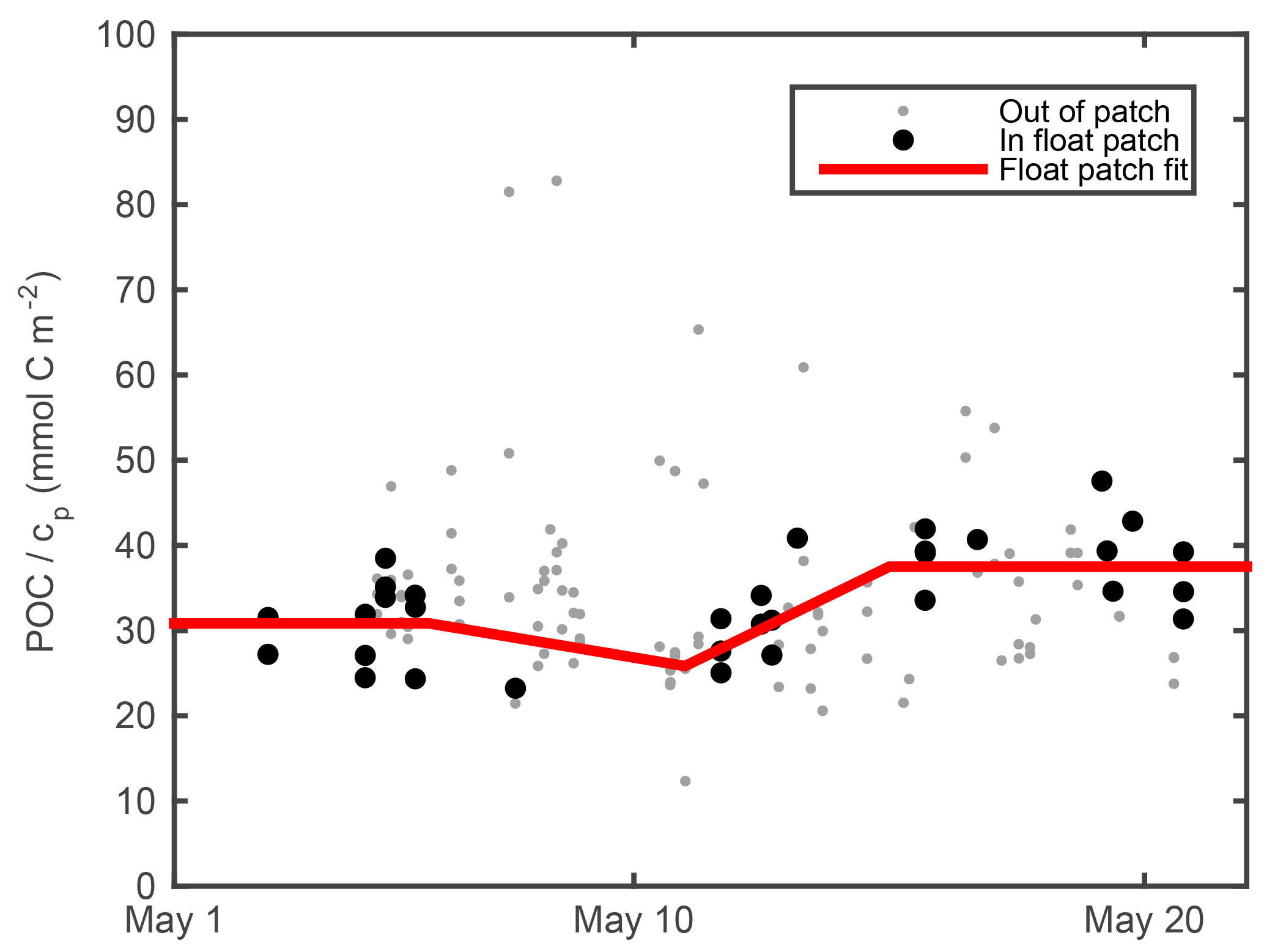
Previous work has shown that measurements of light scattering by particles, including beam attenuation cp and particulate backscattering bbp, correlate strongly with POC in the open ocean (Cetinić et al., 2012, and references therein). Calibration of our cp and bbp measurements and conversion to POC estimates are described in the next two subsections. Raw output from the float optical beam transmissometer was aligned with raw ship transmissometer output using matchups from eight of the calibration casts. Agreement was very good (r2=0.99), showing no evidence of sensor drift. Intercalibrated raw transmissometer output was converted to particulate optical beam attenuation cp using the mean of factory calibrations performed on the ship's transmissometer before and after deployment. More details can be found at http://data.bco-dmo.org/NAB08/C-Star_Calibration-NAB08.pdf, last access: 23 July 2018. We estimated cp-derived POC (POCcp) following Cetinić et al. (2012), but with a time-dependent adjustment in POC ∕ cp ratio to account for community changes. After subtracting the POC ∕ cp regression offset of 0.015 m−1 (Cetinić et al., 2012) from our cp measurements, we computed the POC ∕ cp ratio for all ship POC and cp samples for which cp>0.2 m−1 in the upper 30 m during the May process cruise (Fig. 2; gray points). Samples whose T, S, cp, and bbp matched the float ML measurements within 0.25 ∘C, 0.01 m−1, 0.1 m−1, and 0.001 m−1, respectively, are shown as black circles (Fig. 2). Three inflection points were fit by eye at 370, 310, and 450 mg m−2 on 6, 11, and 15 May, respectively. A continuous estimate of POC ∕ cp at the float patch was obtained by interpolating between these points and assuming constant POC ∕ cp before 6 May and after 15 May (Fig. 2, red line). This continuous estimate of POC ∕ cp was multiplied by float cp (minus offset of 0.015 m−1) to yield a cp-based float POC estimate (POCcp).
2.3.4 POC from optical backscattering
An average of pre- and post-deployment calibrations was used to convert raw backscattering output from both the float and the ship to the volume-scattering function at the angle (140∘) and wavelength (700 nm) of the sensors. The volume-scattering function of seawater was then calculated following Zhang et al. (2009) and subtracted to yield scattering due to particles. The result was multiplied by 2πχ to yield the particulate backscattering coefficient bbp, where the angle-dependent scale factor χ is 1.132 for the FLNTU scattering sensors used in this study (Michael Twardowski, personal communication, 2010). Float bbp was aligned with ship bbp using matchups from eight calibration casts (r2=0.96). More details can be found at http://data.bco-dmo.org/NAB08/Backscatter_Calibration-NAB08.pdf, last access: 23 July 2018. Glider bbp was calibrated against the ship FLNTU in a similar fashion to the float (Briggs et al., 2011). We estimated bbp-derived POC (POCbbp) following Cetinić et al. (2012) via the equation POCbbp [mg C m−3] = 37 500 bbp [m−1] − 14, derived from a linear regression between colocated measurements of POC and bbp within the mixed layer from the May process cruise.
2.3.5 Chlorophyll a
Raw chlorophyll fluorometer output from the ship was converted to an initial Chl a estimate Chl afactory using the factory-calibrated scale factor and a dark offset derived from the minimum of all per-cast deep values (defined as the median between 550 and 580 m). An empirical fit between Chl afactory, T, PAR, and ship discrete Chl a measurements was used to derive an in situ Chl a product
which was strongly correlated with discrete Chl a (r2=0.87). Float Chl afactory was aligned with ship Chl afactory, using the matchups from eight calibration casts (r2=0.95), allowing for the calculation of Chl a via Eq. (1) at the float as well. The FLNTU sensor was located at the bottom of the float, facing down, so Chl a data were removed whenever the float was moving upward at > 1.7 cm s−1 due to the possible entrainment of deeper water. Chl a measurements in which PAR > 75 were also removed to eliminate non-photochemical quenching. In order to obtain a continuous, depth-resolved record of Chl a for the calculation of primary productivity, the remaining Chl a estimates, from both mixed-layer mode and profiles, were filtered using a 5-point running median, averaged in 1 h, 1 m bins, and then interpolated in depth and time via triangulation-based 2-D linear interpolation, with distance calculated as (i.e., a 30 m vertical interval and a 1-day time interval were considered equidistant).
2.3.6 Nitrate
A post-deployment laboratory calibration, including temperature and salinity corrections, was used to obtain initial NO3 estimates from the float's ISUS NO3 sensor. An additional scale factor of 1.15 and offset of +2.6 µM were required to bring these initial estimates in line with discrete samples taken during calibration casts. More details can be found in Alkire et al. (2012) and at http://data.bco-dmo.org/NAB08/ISUS_Nitrate_Calibration-NAB08.pdf, last access: 23 July 2018.
2.3.7 Silicate
SiO4 was not measured by the float, but discrete shipboard SiO4 measurements from the top 15 m were considered to represent mixed-layer SiO4 at the float location if the corresponding temperature, salinity, and NO3 measurements matched concurrent float ML measurements to within 0.25 ∘C, 0.01, and 0.8 mmol m−3, respectively.
2.3.8 PAR
The factory calibration of the float PAR sensor was used “as is.”
2.4 Mixed-layer depth
Mixed-layer depth (MLD) was calculated at hourly intervals from float potential density anomaly estimates via the following steps. (1) Smooth density time series using a 5-point running median. (2) Average density into 1 h, 1 m bins. (3) Fill in the gaps with 2-D linear interpolation such that a 30 m vertical interval and a 1-day time interval are considered equidistant. (4) For each hour, find the minimum potential density anomaly. (5) The MLD for each hour is defined as the shallowest depth at which the potential density anomaly exceeds this minimum by ≥ 0.01 kg m−3. The MLD was calculated twice, once excluding data when downward velocity exceeded 1 m min−1 and once excluding upward velocity exceeding 1 m min−1. We use the average of these two estimates as the final MLD estimate, reducing the influence of single active profiles, which could differ from mean conditions due to entrainment or internal waves. When the float was close to neutral buoyancy, this MLD(t) estimate followed the lower limit of the vertical movement of the float during its ML mode. However, during periods of positive buoyancy, MLD(t) occasionally exceeded the maximum depth of the float during its ML mode (Fig. 3). Hourly MLD depth was also calculated using the same criteria from the output of the Bagniewski et al. (2011) data assimilation model (see red line in Fig. 3) to permit the testing of diel cycle method within the model itself.
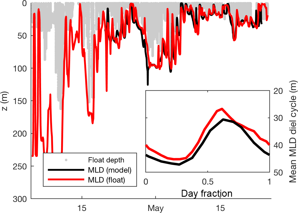
Figure 3Hourly mixed-layer depth estimates calculated directly from float density measurements and from the Bagniewski et al. (2011) data assimilation model (black line), along with the depth of the float in mixed-layer mode (red line). Inset shows mean MLD diel cycle over the entire duration of the model (21 April–24 May). All MLD estimates use a density threshold of 0.01 kg m−3 to better approximate active mixing on an hourly timescale.
2.5 KPAR
2.5.1 Instantaneous KPAR estimates
The diffuse attenuation coefficient of PAR KPARwas calculated from each pair of consecutive PAR measurements made at times t1 and t2 via Eq. (2), where z is depth, is the mean of z(t2) and z(t1), and is the mean of t2 and t1.
2.5.2 KPAR fit method
The uncertainty of individual KPAR(measured) estimates was high and depended strongly on dz, which ranged from 0.2–30 m with a mean of 1.3 m. These 14 000 KPAR(measured) estimates were therefore fit to Chl a and z using a nonlinear least squares multiple regression weighted by dz to obtain Eq. (3):
In order to evaluate the performance of this fit, KPAR(measured) precision was increased by eliminating estimates with dz<2 m and combining the remaining estimates into 21-point medians, yielding a total of 118 independent in situ KPAR estimates. A type-II linear regression of these estimates against 21-point medians of KPAR estimated via Eq. (3) yielded an r2 of 0.85, a root mean square error of 0.014 m−1, and a mean bias of −0.004 m−1. The residual error was not significantly correlated with depth, time, solar zenith angle, or the ratio of in situ Chl a to bbp, a proxy for the plankton community in this system (Cetinić et al., 2015).
2.6 Depth-resolved PAR
In order to calculate PAR at all depths, PAR was extrapolated from a reference depth zref via Eq. (4):
using KPAR(modeled) calculated via Eq. (3) from the float's continuous Chl a. When the float was within the top 50 m, zref was the depth of the float and PAR(zref) was the float's PAR measurement. The performance of this extrapolation was evaluated by comparing PARextrapolated(0−) (just below the surface) calculated via Eq. (4) with scalar PAR(0+) measured by the ship's underway system. For all measurements during which the ship was within 1 km of the float, the float was in the top 50 m, and PAR(0+) was greater than 1 , PAR(0+) and PARextrapolated(0−) were highly correlated (r2=0.96 on a linear scale and r2=0.99 on a logarithmic scale). The geometric mean of the ratio of PARextrapolated(0−) to PAR(0+) was 0.92 and the geometric (multiplicative) standard deviation was a factor of 1.19. For several hours each afternoon, while the float profiled to 250 m, float PAR measurements were not available, so PAR(0−) was estimated using an empirical function of solar zenith angle and an empirical index of cloud cover. First, a double exponential was fit to 36 000 PAR measurements obtained in the top 1 m over a range of solar zenith angle θ from −6 to 90∘ by a global network of 100 Biogeochemical-Argo-type profiling floats to obtain PARmodeled(0−), an estimate of PAR(0−) under mean cloud and atmospheric conditions:
To adjust for clouds, PARextrapolated(0−) from the Lagrangian float (via Eq. 4) was divided by corresponding estimates PARmodeled(0−) to obtain an index of sunniness, which was averaged into 15 min bins to remove noise from wave focusing. This sunniness index ranged from 0.1 to 3.6 over the entire float deployment. Sunniness index at time t was estimated using a ± 1-day running mean of these sunniness index estimates weighted by the inverse square of t−ti, where ti is the time of each measurement. This running mean sunniness index was then multiplied by PARmodeled(0−) to obtain PARadjusted(0−), which was used as PAR(zref) in Eq. (4) during the afternoon gaps.
2.7 O2 air–sea flux
O2 air–sea flux was calculated following Alkire et al. (2012). Briefly, wind speeds were taken from the NCEP WW3 Global Reanalysis product, except during the May cruise, when ship wind measurements were used. O2 saturation was calculated following García and Gordon (1992). Air–sea flux was calculated following Wanninkhof (1992), modified to account for bubble injection following Woolf and Thorpe (1991). Hourly dO2∕dt in the ML due to air–sea flux was estimated by dividing hourly flux estimates by hourly MLD.
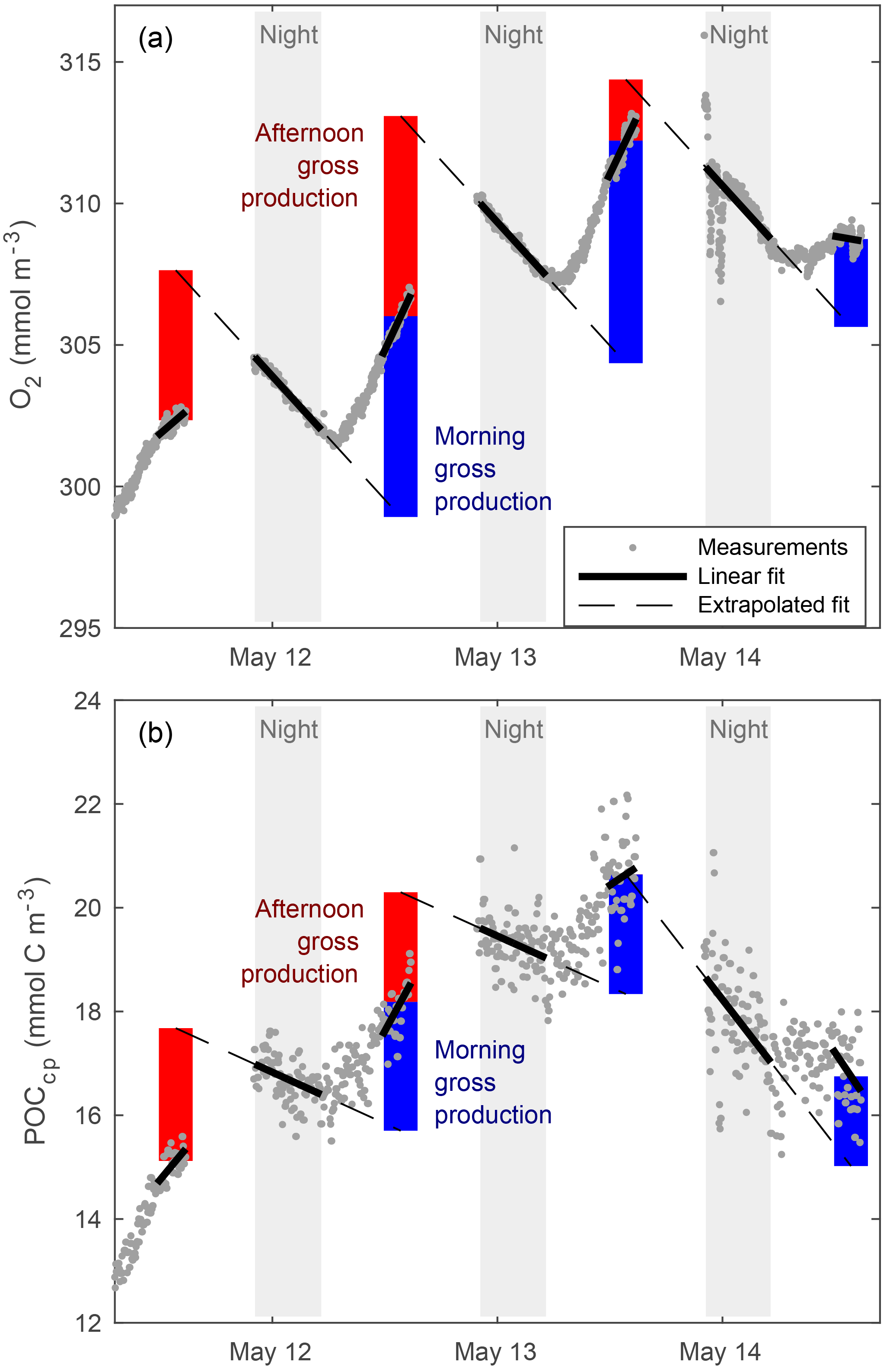
Figure 4Calculation of the gross production of O2 (a) and POCcp (b) in the ML from their diel cycles.
2.8 Primary productivity estimates
2.8.1 Diel cycles of O2 and POC
“Typical” diel cycles (minimum near dawn and maximum near dusk) were observed in mixed-layer records of O2 (Fig. 4), consistent with previous studies (Caffrey, 2003; Hamme et al., 2012; Nicholson et al., 2015). We estimated mixed-layer gross oxygen productivity (GOP) at half-day intervals from these diel cycles. To estimate morning GOP, ML O2 concentrations were smoothed with a 3-point running median, and a type-I linear regression (O2 vs. time) was fit to data from dusk to dawn (Fig. 4a; solid black line). The regression fit was projected forward to provide an estimate of noontime mixed-layer O2 in the absence of GOP. Measured noontime O2 was calculated from a type-I linear regression of O2 data taken within 1 h of local noon. Morning mixed-layer GOP was calculated as the difference between measured and projected concentration (Fig. 4; blue vertical bar) and divided by 0.5 days to convert to units of . Afternoon GOP was calculated in a similar fashion, by subtracting noontime mixed-layer O2 from the noontime extrapolation of a linear fit of the following night's data. Similar diel cycles were observed in mixed-layer POCcp, and the same method was used to calculate the mixed-layer gross primary productivity of POC (GPPcp) from these cycles (Fig. 4b). Diel cycles in POCbbp were less regular and usually out of phase with O2 and POCcp cycles, but GPPbbp was calculated in the same way as GOP and GPPcp for comparison. Note that this diel cycle method assumes homogeneous mixing to a constant depth and that any gain or loss terms other than GOP (or GPP) are constant day to night over the period of a single calculation (∼ 18 h). However, we find a clear diel cycle in MLD (Fig. 3), which amplifies the diel cycle in O2 (and cp and bbp), causing PP calculated from diel cycles to exceed mean PP within the daily mean MLD. This is because nighttime ML deepening enhances the loss of ML concentration relative to daytime mixing losses. Analysis of the output of a coupled physical–biological model assimilating data from the Lagrangian float (Bagniewski et al., 2011), which accurately reproduced the diel cycle in mixing (Fig. 3, black line), shows that the mixing-amplified diel cycles of O2 in the ML yield daily GOP estimates that correspond approximately to the mean GOP above the daily minimum MLD. Regression of diel GOP, calculated from ML O2 time series output by the model as a function of “true” model GOP forced through zero, yields a slope ± 95 % confidence interval of 0.91 ± 0.12 and an RMSE of 0.12 . We therefore interpret our daily GOP and GPPcp estimates as representing daily mean productivity between the surface and daily minimum MLD. Bias in GOP due to day–night differences in air–sea flux was also estimated using the difference between mean morning (or afternoon) dO2∕dt due to air–sea flux and that of the previous (or next) nighttime. Mean bias was small (< 5 % of GOP) and linked primarily to the MLD diel cycle, so a separate correction was not deemed necessary. Other potential biases are discussed in Sect. 4.1.2 to 4.1.4.
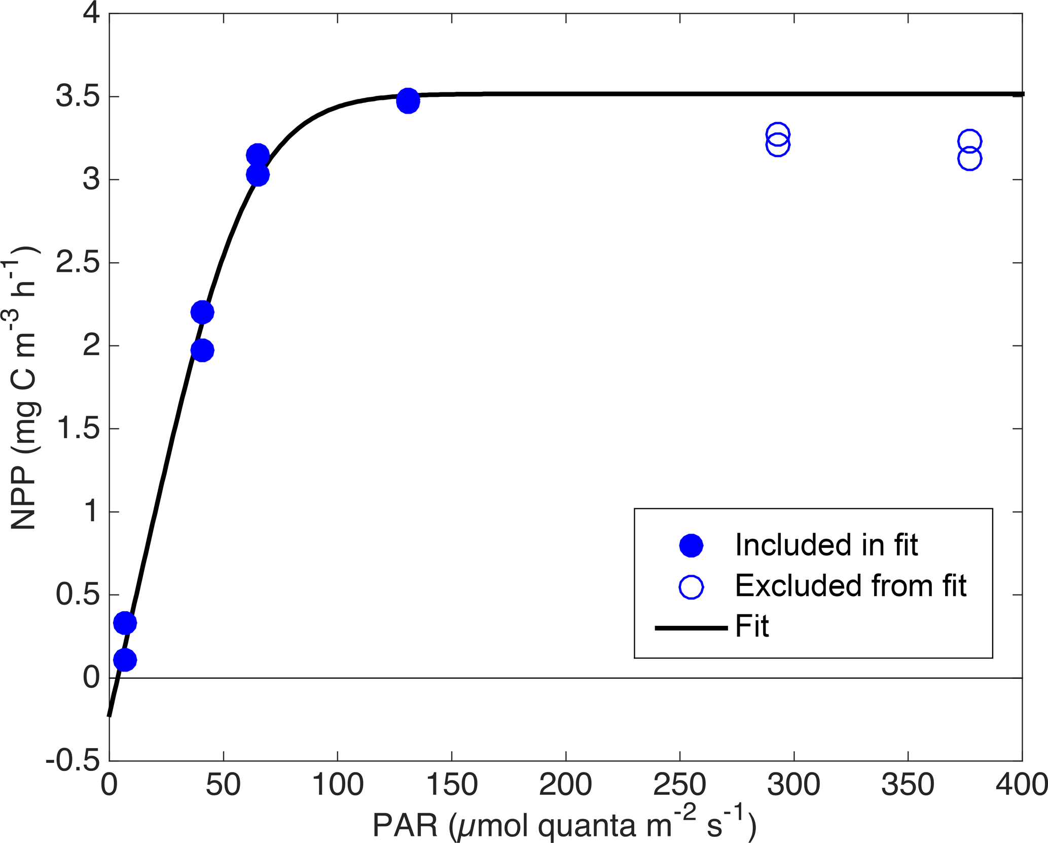
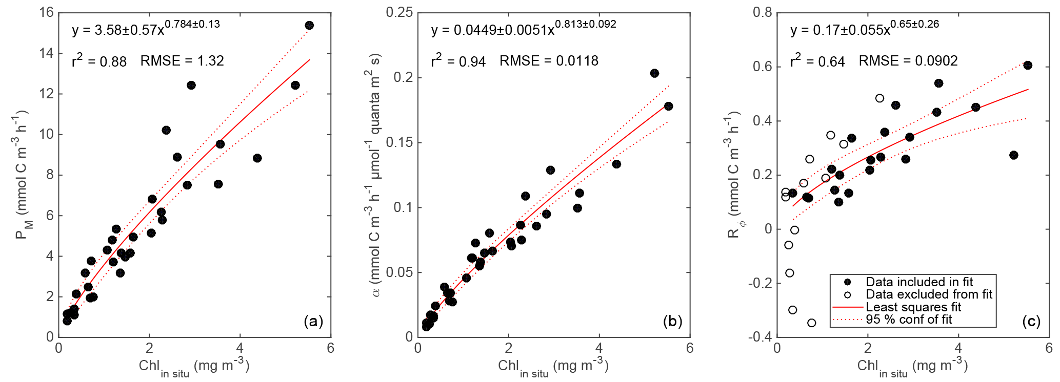
Figure 6Photosynthetic parameters Pm (a), α (b), and RΦ (c) vs. in situ Chl a with least squares power-law fits and 95 % confidence intervals. RΦ estimates from April and June cruises are excluded from fit (panel c, open circles).
2.8.2 14C incubations
During the April and May cruises, daily 2 h 14C incubation experiments were conducted (n=28) to estimate photosynthetic parameters. Each day, a water sample was taken from the Chl a maximum, as determined by in situ fluorescence, and duplicate 2 h 14C incubations were carried out at seven different PAR levels ranging from 0–400 . The dark incubation 14C activities were weakly but significantly correlated with Chl a (type-II linear regression; r2=0.19; p<0.05; apparent NPP = Chl a⋅0.036 ± 0.026 + 0.049±0.035 ); dark activities were treated as sample-specific blanks and subtracted from the light incubation activities of the corresponding water sample. The resulting productivity estimates were interpreted as net primary productivity (NPP) based on findings that most phytoplankton do not respire old carbon when newly fixed carbon is available (Marra and Barber, 2004; Pei and Laws, 2013). Note that if, contrary to our assumptions, phytoplankton did respire old carbon at all light levels during these incubations, then our calculations below overestimate NPP and underestimate phytoplankton respiration (RΦ), but GPP is unbiased. On the other hand, if old carbon is respired only in the low light incubations, then we underestimate RΦ and GPP, but little bias is introduced in NPP. Seven of the 350 individual NPP estimates (all from the April cruise) were judged to be positive outliers and were manually removed before further analysis. In ∼ 60 % of the incubation experiments, NPP decreased with increasing PAR for PAR > 200 . We conclude that this apparent photoinhibition is likely not representative of most field conditions because in situ measurements of Chl a-normalized dO2∕dt showed no consistent relationship with PAR between PAR values of 100 and 1000 . We therefore removed values of NPP in which PAR > 200 if they were lower than the second-highest NPP observed in which PAR < 200 (56 of 110 high light points removed). Remaining NPP vs. PAR data were fit to an empirical “PvE” model represented in Eqs. (6)–(8):
based on four parameters: maximum GPP (Pm), the initial slope of GPP ∕ PAR (α), RΦ, and an efficiency factor (ε) representing the “sharpness” of the transition between light-limited and light-saturated photosynthesis. This parameterization is based on a conceptual model of photosynthesis in which there is a rate-limiting step that can receive and “store” up to ε “packets” of energy at once at above the limiting rate without wasting any of these packets. We used a single ε value of 6, which provided the best overall least-squared fit across all incubation experiments. This ε value yields an NPP vs. PAR relationship that is “sharper” than the commonly used “tanh” model (Harrison and Platt, 1986) and more linear at low PAR, leading to smaller y offset (smaller RΦ estimate). See Fig. 5 for example fits. A power law was then fit between in situ Chl a estimates from the ship's profiling package (calculated via Eq. 1) and each of the three parameters obtained from each NPP vs. PAR fit (Pm: Fig. 6a; α: Fig. 6b; and RΦ: Fig. 6c). Fits with Pm and α used data from all cruises, but the fit with RΦ included only data from the process cruise (Fig. 6c; solid circles), as signals were too low to constrain RΦ in April and RΦ appeared consistently higher during the June cruise, possibly due to higher temperature.
2.8.3 Chl a-based GPP and NPP
The relationships in Fig. 6 were used to estimate photosynthetic parameters Pm(t,z), α(t,z), and RΦ(t,z) and their uncertainty intervals at the float location from Chl a(t,z) (Sect. 2.3.5). We estimated gross primary productivity GPPChl a(t,z) and net primary productivity NPPChl a(t,z) via Eqs. (6)–(8) using the above photosynthetic parameters, PARextrapolated(t,z) (Sect. 2.6), and ε=6 as input. Uncertainties were propagated from Pm(t,z), α(t,z), and RΦ(t,z) using the conservative assumption that they covary (i.e., upper bound of NPPChl a was derived from upper bounds of Pm and α and lower bound of RΦ).
2.9 Area-weighted mean particle diameter
The area-weighted mean particle diameter Dbbp 10–50 m depth bin was estimated following Briggs et al. (2013) via Eqs. (9)–(11):
where Var[bbp(t)] is the variance in bbp due to the random distribution of particles in space, E[bbp(t)] is mean bbp, V is sensor sample volume, Qbb is the backscattering efficiency, and γ and τ are functions of residence time in the sample volume tres and sample integration time tsamp. Var[bbp(t)] and E[bbp(t)] were calculated once per profile (ascent or descent) using all data between 10 and 50 m. Prior to calculation of Var[bbp(t)], the bbp time series was de-trended by subtracting a 7-point running median and large outliers (greater than 5 times the interquartile range) were removed before the variance was calculated on the residuals. A V of 0.62 mL was used (Briggs et al., 2013) and a Qbb of 0.02 was assumed (based on an empirical bbp∕cp ratio of ∼ 0.01 and theoretical value of Qc=2 for diameter ≫ wavelength; Bohren and Huffman, 1983). A tres of 0.02 s was chosen based on a 6 mm path through the sample volume and a platform velocity of 30 cm s−1, and tsamp was 1 s.
2.10 Sinking POC flux
POCbbp profiles from both gliders and the float were divided into a “small” particle baseline (7-point running minimum followed by running maximum) and a “large” particle “spike” signal (residuals above the baseline). This approach, developed by Briggs et al. (2011), is based on the finding that large, fast-sinking particles, owing to their rarity and light-scattering characteristics, can create individual large spikes in mesopelagic bbp clearly distinguishable from background concentrations (Briggs et al., 2011). Large particle POCbbp was multiplied by a bulk sinking speed of 75 m day−1 to estimate large POC flux (Briggs et al., 2011). A broad plausible range of bulk sinking speeds 5 ± 5 m day−1 was used to estimate small POC sinking flux, which was added to large POC flux to yield total sinking POC flux. Sinking POC flux was bin averaged in 50 m vertical bins and either running 2-day bins (gliders) or longer discrete bins to match bloom stages (float).
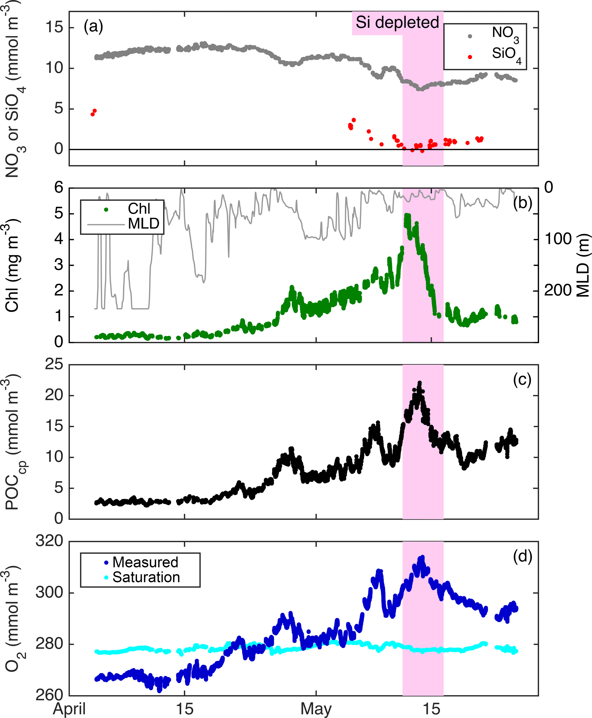
Figure 7Float patch mixed-layer time series of NO3 (a), SiO4 (a), MLD (b), Chl a (b), POCcp (c), O2 (d), and the concentration of O2 saturation (d).
3.1 Evolution of the spring bloom
From float deployment through 17 April, MLD was variable (often > 200 m but occasionally < 50 m; Fig. 3), mixed-layer nutrients were high (NO3≈12 mmol m−3; SiO4≈4 mmol m−3), biomass was low (Chl a ≈ 0.35 mg m−3; POCcp ≈ 35 mg m−3), and O2 was undersaturated by ∼ 10 mmol m−3 (Fig. 7). Mixed-layer biomass concentrations increased over the next month, peaking in mid-May. This broad increase was punctuated by several 1–2-day periods of decrease, most associated with clear mixed-layer deepening (Fig. 7). SiO4 was depleted to its lowest level on 11 May, Chl a concentration peaked on 12 May, and NO3 depletion and POCcp and O2 concentrations peaked on 13 May. From bloom peak to 16 May, Chl a decreased dramatically (77 %), POCcp and O2 decreased moderately (by 9 and 13 mmol m−3, respectively), and NO3 and SiO4 concentrations recovered slightly (by 0.8 and 0.4 mmol m−3, respectively).
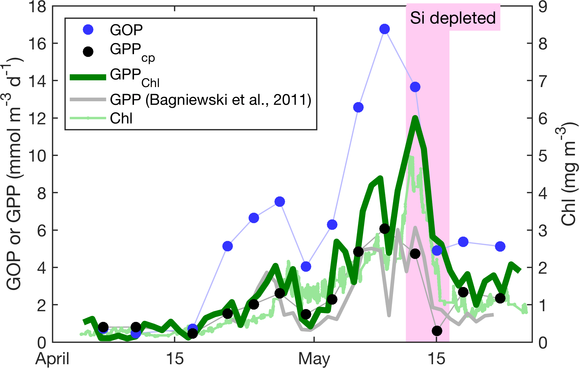
Figure 8Primary productivity estimates within the daily minimum ML. GPPChl a, GOP, GPPcp, and GPP from Bagniewski et al. (2011), along with ML Chl a. Diel-cycle-based estimates are 3-day means; other productivity estimates are daily, and Chl a is continuous.
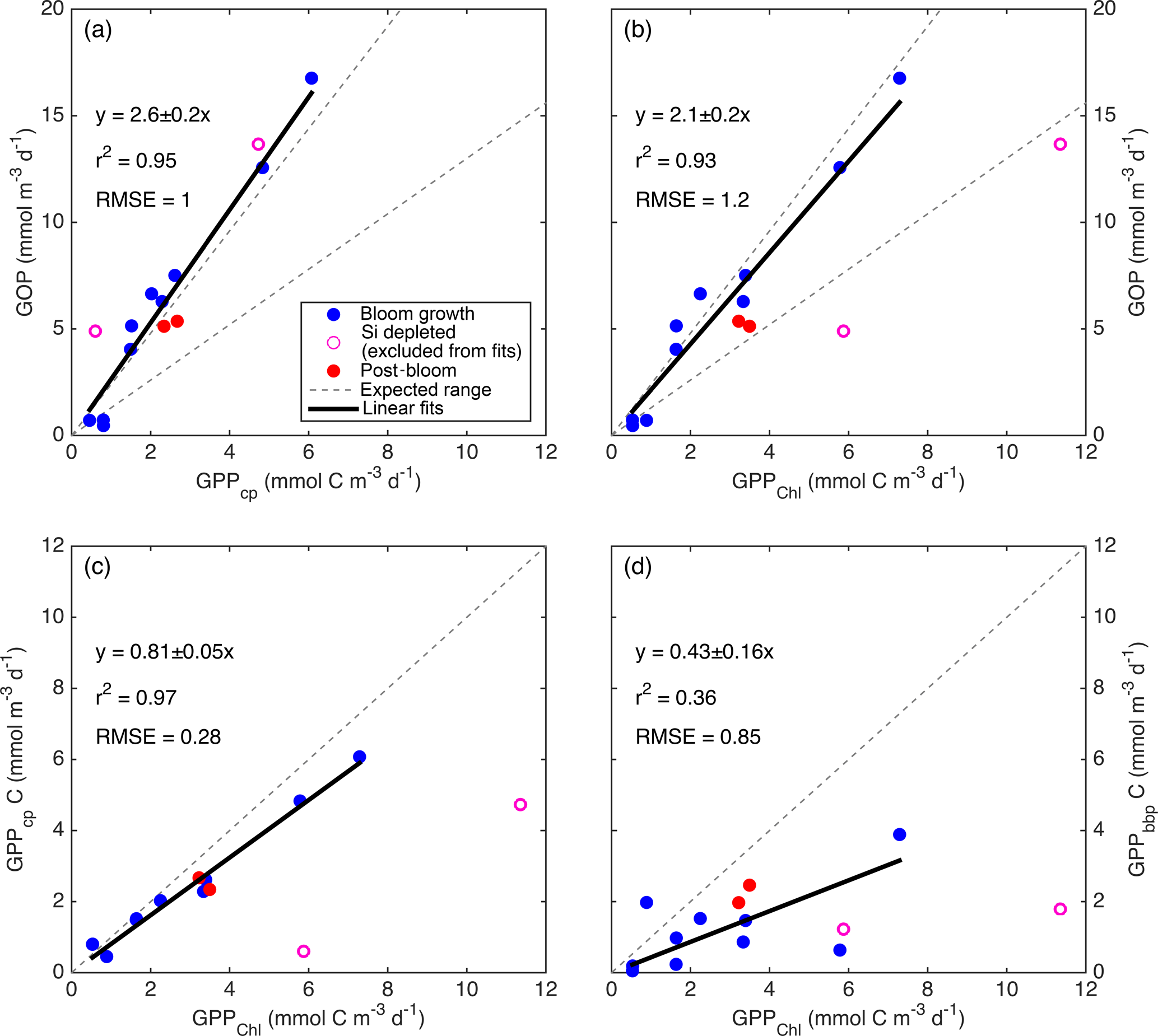
Figure 9Relationships between primary productivity estimates: GOP vs. GPPcp (a), GOP vs. GPPChl a (b), GPPcp vs. GPPChl a (c), and GPPbbp vs. GPPChl a (d). Type-I linear regressions are forced through the origin and include all data except the SiO4-depleted period (pink circles). The expected range of GOP ∕ GPP (a, b; dashed lines) assumes a photosynthetic quotient between 1–1.45 and 22–40 % of fixed carbon released as DOC (see text).
3.2 Primary productivity estimates
All GPP and GOP estimates were averaged into 3-day bins to improve the precision of the diel-cycle-based estimates. To first order, GPPChl a followed Chl a by being low in early April (0.5–1.0 ), peaking near 10 between 7 and 13 May, then decreasing to near 3 or below after the bloom (Fig. 8). But increases in GPPChl a preceded increases in Chl a by 1–2 days during ML shoaling (and high growth) events on 24–27 April and 6–8 May (Fig. 8; pale vs. dark green) due to higher ML-averaged PAR (not shown). For the entire “bloom growth” phase from early April through 9 May, GPPChl a was strongly correlated with both cycle-based estimates of both GOP (Figs. 8 and 9b; blue) and GPPcp (Figs. 8 and 9c; blue). GOP was a factor of 2.1 higher than GPPChl a on a molar basis, while GPPcp was slightly lower (factor of 0.81). GPPbbp was poorly correlated with GPPChl a and significantly lower (by 60 %; Fig. 9d). From noon 10 May to noon 11 May, diel cycles could not be calculated because the float was trapped at the surface due to high stratification and slight positive buoyancy. At peak biomass (11–13 May), and the bloom decline (13–16 May), both GOP ∕ GPPChl a and GPPcp ∕ GPPChl a were substantially lower than during bloom growth (Fig. 8, pink highlighted region, and Fig. 9, pink symbols). In the post-bloom period (16–24 May), GOP ∕ GPPChl a and GPPcp ∕ GPPChl a increased again, similar to the bloom growth ratios (Figs. 8 and 9; red symbols). When all bloom phases are combined, best-fit ratios of GOP and GPPcp to GPPChl a are 1.7 and 0.6, respectively, and correlations are considerably less strong (r2 of 0.67 and 0.49, respectively). However, the estimates of productivity from diel cycles (GOP and GPPcp) remained strongly correlated for the entire deployment. Over the entire study period, morning estimates of GOP and GPPcp were not significantly different from the afternoon estimates, while morning GPPbbp estimates were significantly lower than afternoon estimates (80 % lower overall). However, morning–afternoon patterns appear to change starting on 13 May, when the bloom decline starts (e.g., Fig. 4). From 13–24 May, there is no significant difference between morning and afternoon GPPbbp, but afternoon estimates of GPPcp and GOP were lower than morning estimates by 70 and 43 %, respectively. These differences were near the threshold of statistical significance: mean afternoon–morning difference ± 2 standard errors was −2.3 ± 2.3 for GPPcp and −3.0 ± 2.5 for GOP.
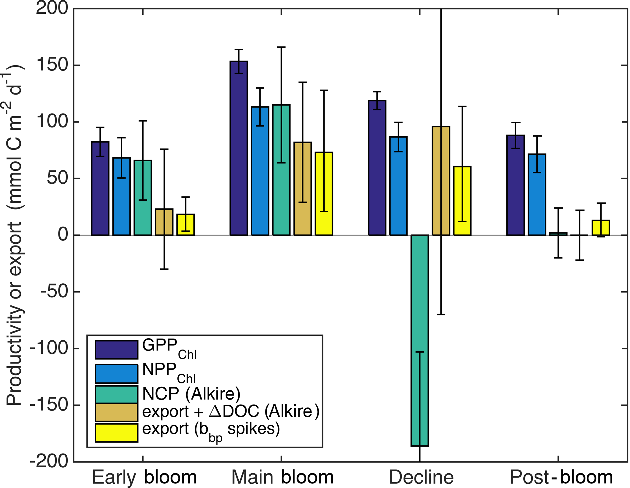
Figure 10Estimates of sources and sinks of organic carbon integrated over the top 60 m: GPPChl a and NPPChl a and sinking particle export (this study), as well as NCP and loss due to the sum of sinking particle export and net DOC production and sinking particle export only (Alkire et al., 2012). Bloom periods follow Alkire et al. (2012) and are defined in the text (Sect. 3.3).
3.3 Depth integrated GPP, NPP, and NCP and carbon export
Alkire at al. (2012) estimated net community productivity (NCP) integrated within the top 50–60 m and carbon export from 50–60 m at the float location for four periods of stable stratification: the “early bloom” (23–27 April), “main bloom” (6–13 May), “decline” (13–14 May), and “post-bloom” (20–24 May). We integrated GPPChl a and NPPChl a to the same depth and time ranges in order to assemble detailed organic carbon budgets for these periods (Fig. 10). Each budget term carries considerable uncertainty, but based on the central estimates, the partitioning of fixed carbon appeared to change substantially over the course of the bloom. Note that these NCP estimates include the net production of dissolved organic carbon (DOC), while NPPChl a excludes any photosynthetic DOC production. NPPChl a and NCP estimates were similar during the early and main bloom, suggesting moderate to low heterotrophic respiration. During the early bloom period, export was also low (∼ 22–28 % of GPPChl a), allowing for the rapid accumulation of biomass. During the main bloom, GPPChl a nearly doubled as biomass increased, but a larger fraction (∼ 50 %) was exported, leaving ∼ 25 % to accumulate. During the bloom decline, apparent community respiration (defined as the difference between GPPChl a and NCP) was 156 % of GPPChl a and export was an additional 50–80 %. In the post-bloom period, community respiration was again high (∼ 100 % of GPP), and export was much lower (0–15 % of GPP). Our NPPChl a estimates and bbp spike-based sinking flux estimates provide a continuous, high-resolution picture of the link between productivity and export at 125 m for the entire study period (Fig. 11a). Float- and glider-based POC export estimates agree broadly at this depth (red lines), suggesting that the higher-resolution glider time series are representative of the float patch as well. While export at 125 m is coupled with NPPChl a (Fig. 11a), there is a rapid increase in export efficiency between 3 and 6 May from ∼ 20 to 40 %. Area-weighted mean particle diameter (Dbbp) ranged from 90–150 µm during April and peaked at 250 µm on 7–8 May (Fig. 11b), coincident with peak biomass as measured by both Chl a and POCbbp from the gliders (not shown). Dbbp fell rapidly on 9 May, coincident with an ML deepening event. Post-bloom Dbbp ranged from 150–190 µm (Fig. 11b).
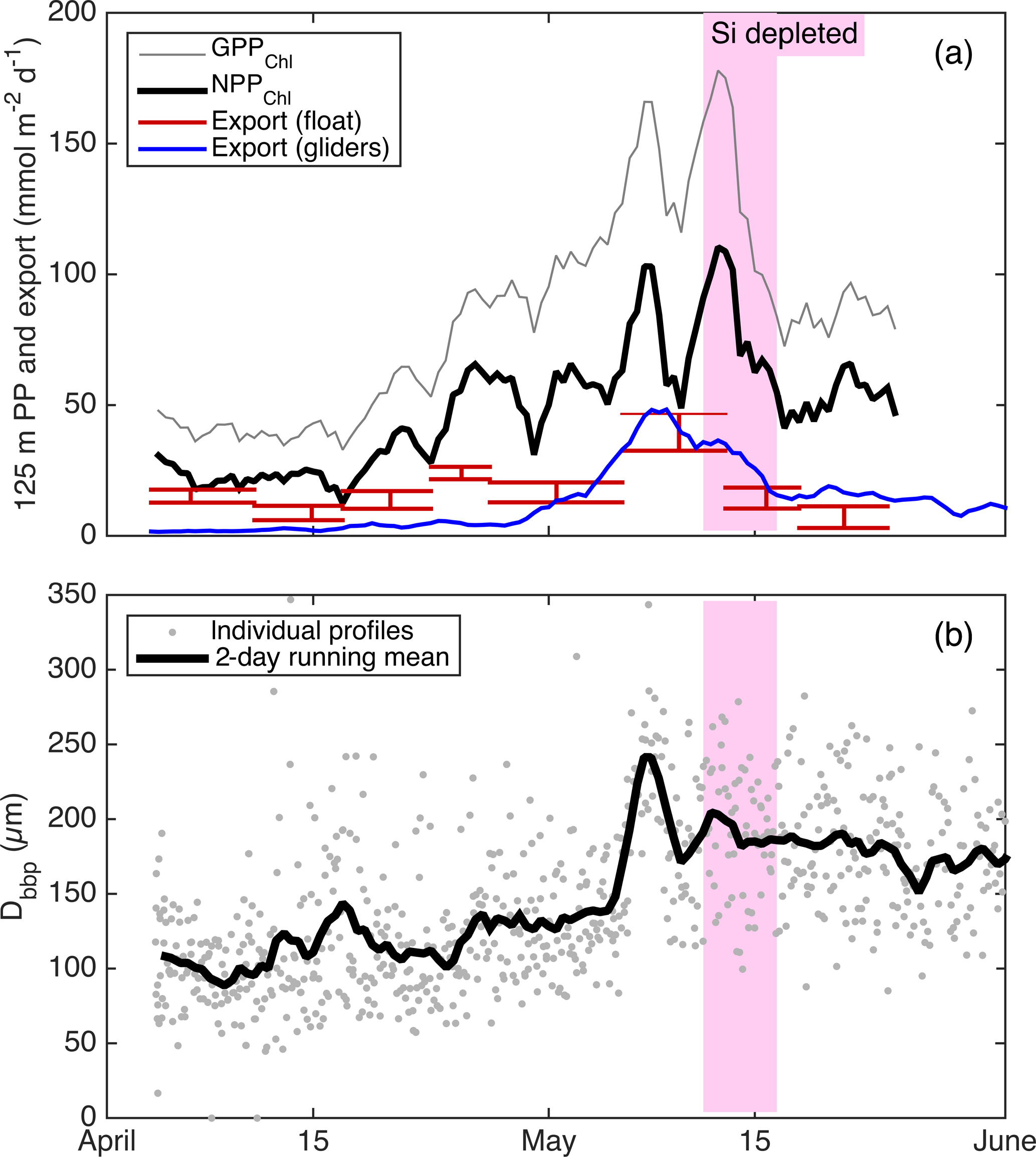
Figure 11(a) Continuous productivity and export from the autonomous float and gliders to and from the top 125 m over the entire study period. Productivity and glider export are 2-day running means, while float export is averaged over longer periods denoted by the width of the bars. Bar height denotes uncertainty bounds. (b) Near-surface glider Dbbp estimates from 10–50 m.
4.1 Accuracy of PP estimates
The combination of three estimates of primary productivity and one estimate of community productivity, all from the same platform at comparable temporal and horizontal scales, provides a unique opportunity to evaluate the accuracy of all methods. Each of our PP methods is discussed in turn in Sect. 4.1.1–4.1.4.
4.1.1 GPPChl a
GPPChl a and GPPcp are estimates of the same quantity obtained independently. GPPChl a is derived from PAR and Chl a estimates using robust local parameterizations obtained from 14C incubations. GPPcp is derived entirely from cp measurements converted to POC using another robust, local empirical relationship. The averaging depth (daily minimum MLD) for GPPChl a was chosen to match the diel cycle method based on the results of a model tuned to match local conditions (Bagniewski et al., 2011). In this context, the combination of strong correlation and absolute agreement between GPPChl a and GPPcp (Fig. 9c; within 19 %) provides confidence in both methods during the bloom growth and post-bloom periods. The GOP ∕ GPPChl a slope of 2.1 (Fig. 9b) is at the upper end of the expected range, providing additional first-order support for GPPChl a accuracy. Neither GPP method includes DOC production, so the range of expected photosynthetic quotients (∼ 1–1.45; Laws, 1991; Robertson et al., 1993), combined with the fraction of GPP released as DOC in marine and estuarine environments (2–50 %; Baines and Pace, 1991), implies a possible GOP ∕ GPP range of 1–2.9. During the main bloom observed by the float in this study, Alkire et al. (2012) estimate that DOC accounts for 22–40 % of NCP in the mixed layer. If these estimates apply to GPP as well, our expected GOP ∕ GPP range narrows to 1.3–2.4 (Fig. 9a, b; gray dashed lines). Thus, our GOP estimates suggest either that both the photosynthetic quotient and phytoplankton DOC production are high during bloom growth (and GPP is accurate) or that both GPP estimates are biased low. As mentioned in Sect. 2.8.2, a negative bias in GPPmodel could be explained if phytoplankton respired substantial old, unlabeled carbon in our low light incubations, but not in the high light incubations. In this case a separate explanation (see next section) is needed for the high GOP ∕ GPPcp slope of 2.6 (Fig. 9a).
During bloom peak and decline, the strong discrepancies between GPPcp and GPPChl a imply either an underestimate by GPPcp (discussed in the next section) or an overestimate by GPPChl a. If diatoms reduce GPP in response to sustained SiO4 limitation, then we expect GPPChl a overestimation at peak biomass given that GPPChl a is only a function of Chl a and PAR, without any nutrient limitation term. Twelve mixed-layer SiO4 samples were collected in the vicinity of the float on 11–13 May, and the mean and maximum measured concentrations were 0.3 and 0.6 mmol m−3, respectively, suggesting that diatom growth was most likely severely limited (Fig. 7a). This does not necessarily imply that diatom carbon fixation rates were reduced, but previous studies have indeed observed a large and reversible reduction in apparent diatom photosynthetic efficiency under multi-day SiO4 limitation (Lippemeier et al., 1999, 2001). Both FlowCAM microscopy and HPLC pigments indicate that diatoms accounted for ≥ 50 % of phytoplankton biomass at bloom peak (Cetinić et al., 2015), so we expect a substantial reduction in bulk phytoplankton growth (and likely GPP) under these conditions. This expectation, combined with the observed reduction in both GPPcp and GOP at bloom peak, leads us to conclude that GPPChl a is most likely overestimated at bloom peak. This conclusion agrees with the coupled physical–biological model of Bagniewski et al. (2011), which assimilated float biogeochemical measurements and achieved optimal fit when diatom GPP was limited by SiO4 with a half-saturation constant of 1 µmol m−3. GPP inferred from this model closely matches our observed GPPcp during SiO4 limitation (Fig. 8, gray line vs. black circles), even though Bagniewski et al. (2011) assimilated daily binned data, removing any diel cycle information. On the other hand, three 14C incubations were conducted between 10 and 14 May using water with SiO4 < 0.5 mmol m−3, although not at the float location, and there was not a substantial reduction in measured Pm. These samples may not be representative of the water sampled by the float, despite similar Chl a and SiO4 concentrations, or it is possible that a bottle effect enhanced GPP. But we cannot rule out the alternative hypothesis that the Si-limited community continued to fix carbon at a constant rate and that GPPcp and GOP estimates were reduced for another reason (discussed in next sections).
Apart from Si limitation, possible explanations for GPPChl a overestimation include overestimation of Chl a due to increased fluorescence, underestimation of the MLD, or photoinhibition. Again, Chl a was calculated the same way for the floats and ship, so if the in situ fluorometric method overestimated Chl a at bloom peak, we would expect to see a deviation from the observed relationships between photosynthetic parameters and Chl a (Fig. 6). So this explanation, while plausible given the high Chl a ∕ bbp ratio at bloom peak (Cetinić et al., 2015), also requires that none of our low SiO4 bottle samples were representative of the bloom peak at the float location. The density-based MLD estimates appear quite robust during this period, consistently shallow and stable at 10–20 m and matched by the vertical motion of the float. And the daytime increases in O2 (Fig. 4) and cp on 11 and 12 May show no sign of photoinhibition, despite a peak hourly-averaged PAR of > 750 ; increases are smooth throughout the morning and appear to continue at the same rate in the afternoon (Fig. 4). This result supports our decision to exclude photoinhibited bottle incubation data from our productivity vs. PAR fits, and we suggest that photoinhibition terms from bottle incubations should be applied with caution, if at all, in future studies. In this system, photoinhibition is likely reduced during deeper mixing events due to the shorter time phytoplankton is exposed to high light. During the stratified conditions, reduction in photoinhibition can be attributed to photoadaptation.
SiO4 limitation may also explain some of the discrepancy between GPPcp and GPPChl a during the bloom decline (13–16 May), at least when afternoon estimates are excluded (see Fig. 9b, c; open pink circles). Lower afternoon GPPcp and GOP, combined with very shallow (< 5 m) MLDs at noon on 13 and 15 May, also raise the possibility of significant photodamage inhibiting afternoon productivity. Mean ML PAR exceeded 500 for at least 2 h on both days. However, the negative afternoon GPPcp estimates at this time suggest a bias in the diel cycle method as well (see next section).
4.1.2 GPPcp
Potential sources of bias unique to GPPcp include a diel cycle in grazing (e.g., due to diel migration of zooplankton), a diel cycle in export loss, or a diel cycle in the POC ∕ cp ratio. The tight correlations between GPPcp and GOP throughout the entire study period (r2=0.95; Fig. 9a) and between GPPcp and GPPChl a during bloom growth (r2=0.96; Fig. 9b) provide encouraging support for GPPcp as a measure of relative primary productivity at the very least. Furthermore, the quantitative agreement between GPPcp and GPPChl a during both bloom growth and post-bloom (Fig. 9c; slope: 0.82 ± 0.06) is very close to our expected slope of 0.93 from model results (reanalysis of Bagniewski et al., 2011), suggesting that GPPcp accuracy is comparable to other methods across most of the conditions encountered. These findings agree closely with those of White et al. (2017), who find a GPPcp ∕ NPP ratio of 1.1 across a factor of 3 dynamic range of productivities in the subtropical North Pacific, suggesting that GPPcp is either accurate or slightly underestimates true GPP. Taken together, our results are highly encouraging regarding the widespread applicability and accuracy of the GPPcp method. However, it should be noted that our results still may not apply to certain other systems in which different phytoplankton size and/or timing of cell division could alter the diel POC ∕ cp relationship (Dall'Olmo et al., 2011).
If the SiO4 limitation hypothesis is correct, then GPPcp during the bloom peak and morning GPPcp during the bloom decline may be accurate as well. On the other hand, if GPPChl a is accurate during this time, then GPPcp is biased low by ∼ 50 % at this time. It is unclear what might cause such a low bias, especially at bloom peak. Between the afternoon of 11 May and the morning of 13 May, there is no anomaly in the diel cycles of POCcp or O2 (Fig. 10) indicative of daytime mixing, advection, or possible photoinhibition, and there is no change in the relationship between GPPcp and GOP (Fig. 9a; rightmost pink symbol). Without grazing data, we cannot rule out enhanced daytime grazing as a possible explanation, although grazing is generally expected to be higher at night. Alternatively, particularly high photooxidation could potentially dampen O2 diel cycles during this period and perhaps cp diel cycles as well. This hypothesis is supported by laboratory measurements of diatom productivity under nutrient limitation (Spilling et al., 2015), although again we would need to explain why reduced Pm was not observed in our bottle incubations. On the other hand, the afternoon GPPcp estimates during the bloom decline period show a clear example of negative bias in the diel cycle method. On 13, 14, and 15 May (bloom decline), the rates of net POCcp (and O2) accumulation are positive or near zero in the morning but negative each afternoon (e.g., Fig. 4; 13 May). One plausible explanation is horizontal advection of the float relative to the ML during its afternoon profile, causing it to resurface in water with lower biomass. During this period, comparison with ship, autonomous glider, and satellite measurements (Alkire et al., 2012) shows that the float was at the edge of a high biomass (and O2) patch, so advection during this time would most likely cause a loss in POCcp and O2. Note that the afternoon reductions in GPPcp during bloom decline are greater than the afternoon reductions in GOP (e.g., Fig. 4). This result is possible with the horizontal advection and mixing hypothesis alone, but high export combined with a shallow afternoon MLD may also play a role. Shallow MLD enhances the loss of ML concentration for a given export rate, and nighttime mixing can re-entrain some of this export, reducing the ML POC diel cycle relative to the O2 diel cycle.
4.1.3 GOP
The tight fit between GOP and both GPP estimates over most of the study period provides important support for the O2 diel cycle method as a measure of relative primary production in this region. Again, because all estimates were independent and taken at the same scale, and because the 2-month deployment allowed 14 independent matchups at a 3-day timescale spanning a wide range of productivities, this dataset represents the most extensive validation to date of the O2 diel cycle method as a measure of relative primary productivity. Additionally, the overall accuracy of our GOP estimates may be assessed indirectly through comparison with independent ship-based GOP estimates made during the May process cruise (Quay et al., 2012) and through comparison of our GOP ∕ GPP and GOP ∕ NPP ratio estimates with previous estimates from this region. Quay et al. (2012) estimated ML-integrated GOP using measurements of three oxygen isotopes, 16O, 17O, and 18O, taken daily between 3 and 21 May during the process cruise. Mean GOP calculated by this method was 245 . This method integrates over several weeks, so we interpret their estimate to correspond roughly to mean ML depth-integrated GOP between 19 April (2 weeks before the first sample) and 21 May. For comparison, we multiply each half-day GOP estimate by MLD to obtain ML-integrated GOP and obtain an average from 19 April to 21 May of 149 , 40 % lower than the Quay et al. (2012) estimate. However, our estimate integrates to the daily minimum MLD, and while the triple O2 isotope method assumes constant MLD, we expect it to more closely approximate daily maximum MLD in the presence of diel MLD fluctuations given its long integration time. Mean GPPChl a during this period, integrated to the bottom of the daily minimum MLD, is 30 % lower than mean GPPChl a integrated to the daily maximum MLD. If we assume the same relative difference for GOP, we obtain a revised ML-integrated GOP estimate of 213 , 13 % lower than the Quay et al. (2012) estimate. Given the uncertainties associated with the GOP methods and the differing spatiotemporal scales, this result provides first-order support for the accuracy of both methods. Our findings reinforce those of Hamme et al. (2012), who in the Southern Ocean in March–April found that mean ML-integrated GOP calculated via O2 ∕ Ar diel cycles (similar to our method) was 18 % lower than GOP calculated via the triple oxygen isotope method (similar to Quay et al., 2012).
Bender et al. (1992) calculated a GOP ∕ NPP ratio of 2.5 during the spring bloom in the northeast Atlantic using in situ 18O incubations and 24 h 14C incubations. We calculate GOP ∕ NPPChl a as shown in Fig. 9b, but replace GPPChl a with NPPChl a and obtain a best-fit ratio and 95 % confidence interval of 2.4 ± 0.2 for the bloom growth period and 1.7 ± 0.4 for the entire deployment. These fits appear to support the accuracy of both our NPPChl a and GOP estimates during the bloom growth phase, consistent with our other findings. However, our GOP ∕ GPP ratio estimates of 2.6 ± 0.2 (Fig. 9a) and 2.1 ± 0.2 (Fig. 9b) are near or above the high end of our expected range of 1.3–2.4 (see Sect. 4.1.1). As discussed in previous sections, these ratios may be the result of a high photosynthetic quotient and high DOC production combined with a small negative bias in GPPcp. Our GOP estimates may also be too high, but we cannot think of a plausible mechanism that would cause a substantial overestimate of diel-based GOP (but not of GPPcp). Regardless of the source of our high GOP ∕ GPP ratios, they are also consistent with Hamme et al. (2012), who also estimated GPP from on-deck PvE incubations and GOP via O2 ∕ Ar diel cycles, providing a very close methodological comparison in a different environment (autumn, Southern Ocean). They obtain an even higher GOP ∕ GPP ratio of 3.6. However, Hamme et al. (2012) assumed that 1–2 h 14C incubations represent GPP, while we assume that these same incubations represent NPP (when NPP > 0). If our assumption is correct, then their method provides a quantity closer to daytime NPP than GPP. However, even in this case, assuming moderate daytime phytoplankton respiration rates (≤ 30 % of GPP), GOP ∕ GPP during their study was > 2.5, which is in agreement with our estimates. It is also worth noting that related studies comparing diel cycles in O2 and pCO2 measurements (Johnson, 2010; Merlivat et al., 2015), both of which include the effects of DOC production, have found ratios of daytime oxygen production to carbon production that are within the expected range of 1–1.45. These results provide further support for diel-cycle-based O2 production and the hypothesis that DOC production may drive the high GOP ∕ GPP observed in this and other studies (Bender et al., 1992; Hamme et al., 2012).
In total, the available evidence provides first-order support for the accuracy of our diel-cycle-based GOP estimates. Our findings build on important recent work in diverse environments showing that diel cycles in the O2 ∕ Ar ratio yield ML GOP estimates that are consistent with independent GOP estimates (Hamme et al., 2012) and that diel cycles in O2 measurements from autonomous gliders in the subtropical Pacific provide GOP estimates that are a reasonable multiple of independent NPP results (Nicholson et al., 2015). Our results add a third ocean region (springtime North Atlantic) and a third platform (Lagrangian mixed-layer float) in addition to new comparisons with cp and bbp diel cycles.
4.1.4 GPPbbp
Because diurnal variability in bbp can be estimated from geostationary satellites (Neukermans et al., 2012), the ability to accurately estimate GPP from bbp diel cycles would be extremely valuable. While ship-based measurements from NAB08 show that bbp and cp were equally well correlated with POC over the May cruise (Cetinić et al., 2012), the poor matchups we find between GPPChl a and GPPbbp suggest that diel changes are present in POC ∕ bbp and can cause strong, consistent bias in GPPbbp. Our results agree with previous findings that while beam attenuation and forward scattering by phytoplankton increase immediately after they begin to photosynthesize, bbp and side scattering often do not, both in the lab (Ackleson et al., 1993; Poulin et al., 2018) and in the ocean (Kheireddine and Antoine, 2014). These results caution against the use of bbp diel cycles to estimate GPP without further research. However, it is worth noting that our afternoon GPPbbp estimates are reasonably well correlated with GPPChl a (r2=0.63, m=0.75 ± 0.23; data not shown) during the bloom growth period. If this result is found to be robust in other times and places, then a useful estimate of GPP from satellite (and other) bbp time series may be possible. However, even if the bbp diel cycle cannot be used to estimate GPP, it likely contains other useful information, especially in combination with cp and/or O2. If robust relationships between plankton communities and/or physiology and bbp diel cycles can be established (and, ideally, understood mechanistically), then measurements of bbp diel cycles may still provide valuable oceanographic information, whether from in situ platforms or satellites.
4.2 Combined upper layer carbon budgets
Taken together with the Alkire et al. (2012) NCP and carbon export estimates and our adaptation of the Briggs et al. (2011) depth-resolved carbon fluxes, our productivity and bulk particle estimates provide a remarkably detailed, high-resolution picture of carbon flows over the entire spring bloom. From 4–17 April, ML Chl a, POC, and O2 concentrations changed little despite large fluctuations in MLD, while NO3 increased slightly during deep mixing, presumably due to entrainment, but was stable during shallow (< 100 m) mixing. Consistent positive 125 m integrated NPPChl a (Fig. 11a) was therefore likely balanced by heterotrophic respiration. From 18 April to 7 May, ML shoaling events coincided with several pulses of high net growth in POCcp and Chl a (Fig. 7), and the close match between NPPChl a and NCP during these periods (Fig. 10) suggests a minimal role of grazing in regulating this growth. From 6–7 May, all four gliders observed a rapid aggregation event (Fig. 11b) that triggered a dramatic pulse in carbon export, both from the float patch and the broader (∼ 30 km) glider survey area (Fig. 11a; blue and red lines). This pulse sank through the mesopelagic at ∼ 75 m day−1 and was composed primarily of fragile aggregates containing live phytoplankton including Chaetoceros sp. resting spores (Martin et al., 2011; Briggs et al., 2011; Rynearson et al., 2013). This aggregate export was the largest loss term of surface POC during the “main bloom”, reducing the biomass accumulation rate by ≥ 50 % (Fig. 10). While SiO4 limitation has been proposed as a cause of this rapid sinking event (Bagniewski et al., 2011), this aggregation commenced when SiO4 concentrations were still > 2 mmol m−3 (Fig. 7a) and 5 days prior to the ∼ 35 % reduction in GOP and GPPcp that we attribute to SiO4 limitation (pink band in Fig. 11b). The exact cause of this rapid aggregation event is unknown, but likely involves a combination of moderately high particle concentration (POCcp > 10 mmol m−3), weakening of mixing (which could break fragile aggregates), and production of transparent exopolymer particles (Martin et al., 2011; Alkire et al., 2012). The combination of high export and reduced productivity at the end of the diatom bloom (12–14 May) appears to end the ML biomass accumulation. However, we conclude that the subsequent sharp decline in ML Chl a, POCcp, and O2 from 14–15 May (Fig. 7) was probably not the result of a dramatic increase in heterotrophic respiration, as implied by the strong negative NCP estimate (Fig. 10) of Alkire et al. (2012). Our conclusion stems from the nighttime ML O2 loss rates, which do not increase at all between the bloom peak the bloom decline (see Fig. 4a). Instead, the ML O2 decline appears to be caused by further GPP decreases due to continued SiO4 limitation and a decline in Chl a (Fig. 7b, d), likely enhanced by the export of phytoplankton from the shallow ML. The O2 decline (and accelerating Chl a decline) may have been enhanced by the advection of the float relative to the thin surface ML during afternoon profiles (see Sect. 4.1.2), or perhaps an additional light-dependent process, such as photoinhibition or photorespiration (Spilling et al., 2015), nearly eliminated GPP during this time, but only in the afternoons. After the decline of the diatom bloom, the different productivity estimates again provide a consistent picture, this time of top-down control. GOP and GPPcp again show no sign of nutrient limitation (Fig. 9b, c, red symbols), and NPPChl a is apparently balanced by heterotrophic respiration. Glider estimates of sinking POC export were low, but higher than early bloom export, despite similar NPP (Fig. 11a) and higher respiration. This result highlights the decoupling between NCP and export on weekly to monthly timescales in this dynamic system and suggests that biomass and particle size are better predictors of sub-seasonal export dynamics. The changing export efficiencies that we observed (< 15 % through most of April, to ∼ 57 % during the main bloom, to ∼ 33 % in the post-bloom period) provide a complex picture of “the spring bloom”, but still agree broadly with the export ratio of 45 % calculated by Buesseler and Boyd (2009) in the North Atlantic spring bloom using JGOFS data, which is among the highest export efficiencies observed in the open ocean. However, unlike Buesseler and Boyd (2009) and in line with the conclusions of Martin et al. (1993), we see significant flux attenuation in the 100 m below the euphotic zone. For example, 35–48 % of flux is lost between 60 m (Fig. 10) and 125 m (Fig. 11a) during the main bloom.
Our results, placed in the context of previous studies, provide strong support for the diel cycle method as a means to obtain estimates of GOP (from O2) and GPP (from cp) with reasonable accuracy relative to existing methods and enough precision on 3-day timescales to clearly resolve a spring diatom bloom. The range of biomass, mixing regimes, and phytoplankton communities in this study, combined with previous results from the subtropics, suggest that these methods are not overly dependent on particular ocean conditions. Because the diel cycle method is well suited for autonomous platforms, it has the potential to greatly increase our coverage of in situ productivity estimates, providing both direct knowledge of this critical biological rate and greatly enhanced validation datasets for satellite-derived and modeled productivity. Our results also support the use of short-term 14C incubations to parameterize simple PvE models for application to autonomous measurements, at least in the absence of strong nutrient limitation. We find high GOP ∕ GPP ratios of 2.1–2.6 through most of the study, suggesting high DOC production and/or a possible moderate underestimation of GPP by both methods. Finally, combined high-resolution estimates of NPP, particle size, and sinking flux during the North Atlantic spring bloom show strong coupling between the three, modulated by a dramatic increase in export efficiency at bloom peak, apparently due to rapid aggregation.
All data presented in this paper have been submitted to the Biological and Chemical Oceanography Data Management Office (BCO-DMO) and can be accessed from the “North Atlantic Bloom Experiment 2008” project page at https://www.bco-dmo.org/project/2098 (D'Asaro et al., 2018).
| bbp | Particulate optical backscattering coefficient |
| Chl a | Chlorophyll a concentration |
| cp | Particulate optical beam attenuation coefficient |
| Dbbp | Area-weighted mean particle diameter from optical backscattering |
| DOC | Dissolved organic carbon concentration |
| GOP | Gross O2 productivity from O2 diel cycles |
| GPP | Gross primary productivity |
| GPPbbp | GPP from optical backscattering diel cycles |
| GPPChl a | GPP from in situ chlorophyll and light measurements |
| GPPcp | GPP from optical beam attenuation diel cycles |
| JGOFS | Joint Global Ocean Flux Study |
| KPAR | Diffuse attenuation coefficient of PAR |
| ML | Mixed layer |
| MLD | Mixed-layer depth |
| NPP | Net primary productivity |
| NPPChl a | NPP from in situ chlorophyll and light measurements |
| PAR | Photosynthetically available radiation |
| Pm | Maximum GPP (light saturated) |
| POC | Particulate organic carbon concentration |
| POCbbp | POC from optical backscattering |
| POCcp | POC from optical beam attenuation |
| PP | Primary productivity |
| RΦ | Phytoplankton respiration rate |
| S | Salinity |
| T | Temperature |
| α | Initial slope GPP ∕ PAR (light limited) |
| ε | Coefficient representing the “sharpness” of the NPP vs. PAR relationship |
The authors declare that they have no conflict of interest.
The collection of data for this study was funded by the US National Science
Foundation (grants OCE-0628107 and OCE-0628379) and NASA (grants NNX-08AL92G
and NNX-10AP29H). Analysis and writing was further funded by a University of
Maine Doctoral Research Fellowship, National Science Foundation
grant OCE-1420929,
and a European Research Council grant. The authors would also like
to thank Andrew Thomas and Emmanuel Boss for valuable comments and feedback
as PhD committee members and the crew and technicians of the RV Knorr and RV Bjarni Saemundsson for
making this entire study possible. We would also like to thank two anonymous
reviewers for their feedback, which has substantially improved this
paper.
Edited by: Gerhard Herndl
Reviewed by: two anonymous referees
Ackleson, S. G., Cullen, J. J., Brown, J., and Lesser, M.: Irradiance-Induced Variability in Light Scatter from Marine Phytoplankton in Culture, J. Plankton Res., 15, 737–759, 1993.
Alkire, M. B., D'Asaro, E., Lee, C., Perry, M. J., Gray, A., Cetinić, I., Briggs, N., Rehm, E., Kallin, E., Kaiser, J., and González-Posada, A.: Estimates of Net Community Production and Export Using High-Resolution, Lagrangian Measurements of O2, , and POC through the Evolution of a Spring Diatom Bloom in the North Atlantic, Deep-Sea Res. Pt. I, 64, 157–174, https://doi.org/10.1016/j.dsr.2012.01.012, 2012.
Bagniewski, W., Fennel, K., Perry, M. J., and D'Asaro, E. A.: Optimizing models of the North Atlantic spring bloom using physical, chemical and bio-optical observations from a Lagrangian float, Biogeosciences, 8, 1291–1307, https://doi.org/10.5194/bg-8-1291-2011, 2011.
Baines, S. B. and Pace, M. L.: The Production of Dissolved Organic Matter by Phytoplankton and Its Importance to Bacteria: Petterns across Marine and Freshwater Systems, Limnol. Oceanogr., 36, 1078–1090, https://doi.org/10.4319/lo.1991.36.6.1078, 1991.
Bender, M., Ducklow, H., Kiddon, J., Marra, J., and Martin, J.: The Carbon Balance during the 1989 Spring Bloom in the North Atlantic Ocean, 47∘ N, 20∘ W, Deep-Sea Res. Pt. I, 39, 1707–1725, 1992.
Bohren, C. F. and Huffman, D. R.: Absorption and Scattering of Light by Small Particles, John Wiley & Sons, New York, 1983.
Briggs, N., Perry, M. J., Cetinić, I., Lee, C., D'Asaro, E., Gray, A. M., and Rehm, E.: High-Resolution Observations of Aggregate Flux during a Sub-Polar North Atlantic Spring Bloom, Deep-Sea Res. Pt. I, 58, 1031–1039, https://doi.org/10.1016/j.dsr.2011.07.007, 2011.
Briggs, N. T., Slade, W. H., Boss, E., and Perry, M. J.: Method for Estimating Mean Particle Size from High-Frequency Fluctuations in Beam Attenuation or Scattering Measurements, Appl. Optics, 52, 6710–6725, 2013.
Buesseler, K. O. and Boyd, P. W.: Shedding Light on Processes That Control Particle Export and Flux Attenuation in the Twilight Zone of the Open Ocean, Limnol. Oceanogr., 54, 1210–1232, 2009.
Caffrey, J. M.: Production, Respiration and Net Ecosystem Metabolism in U.S. Estuaries, in: Coastal Monitoring through Partnerships, edited by: Melzian, B. D., Engle, V., McAlister, M., Sandhu, S., and Eads, L. K., Springer, Springer Science and Business Media, Dordrecht, the Netherlands, 81, 207–219, https://doi.org/10.1007/978-94-017-0299-7_19, 2003.
Cetinić, I., Perry, M. J., Briggs, N. T., Kallin, E., D'Asaro, E. A., and Lee, C. M.: Particulate Organic Carbon and Inherent Optical Properties during 2008 North Atlantic Bloom Experiment, J. Geophys. Res., 117, C06028, https://doi.org/10.1029/2011JC007771, 2012.
Cetinić, I., Perry, M. J., D'Asaro, E., Briggs, N., Poulton, N., Sieracki, M. E., and Lee, C. M.: A simple optical index shows spatial and temporal heterogeneity in phytoplankton community composition during the 2008 North Atlantic Bloom Experiment, Biogeosciences, 12, 2179–2194, https://doi.org/10.5194/bg-12-2179-2015, 2015.
Claustre, H., Morel, A., Babin, M., Cailliau, C., Marie, D., Marty, J. C., Tailliez, D., and Vaulot, D.: Variability in Particle Attenuation and Chlorophyll Fluorescence in the Tropical Pacific: Scales, Patterns, and Biogeochemical Implications, J. Geophys. Res.-Oceans, 104, 3401–3422, https://doi.org/10.1029/98jc01334, 1999.
Cullen, J. J., Lewis, M. R., Davis, C. O., and Barber, R. T.: Photosynthetic Characteristics and Estimated Growth Rates Indicate Grazing Is the Proximate Control of Primary Production in the Equatorial Pacific, J. Geophys. Res., 97, 639, https://doi.org/10.1029/91JC01320, 1992.
Dall'Olmo, G., Boss, E., Behrenfeld, M. J., Westberry, T. K., Courties, C., Prieur, L., Pujo-Pay, M., Hardman-Mountford, N., and Moutin, T.: Inferring phytoplankton carbon and eco-physiological rates from diel cycles of spectral particulate beam-attenuation coefficient, Biogeosciences, 8, 3423–3439, https://doi.org/10.5194/bg-8-3423-2011, 2011.
D'Asaro, E. A.: Performance of Autonomous Lagrangian Floats, J. Atmos. Ocean. Tech., 20, 896–911, 2003.
D'Asaro, E., Lee, C., and Perry, M. J.: Data from the North Atlantic Bloom 2008 project, Biological and Chemical Oceanography Data Management Office (BCO-DMO), https://www.bco-dmo.org/project/2098, last access: 24 July 2018.
García, H. E. and Gordon, L. I.: Oxygen Solubility in Seawater: Better Fitting Equations, Limnol. Oceanogr., 1307–1312, https://doi.org/10.4319/lo.1992.37.6.1307, 1992.
Gernez, P., Antoine, D., and Huot, Y.: Diel Cycles of the Particulate Beam Attenuation Coefficient under Varying Trophic Conditions in the Northwestern Mediterranean Sea: Observations and Modeling, Limnol. Oceanogr., 56, 17–36, https://doi.org/10.4319/lo.2011.56.1.0017, 2011.
Hamme, R. C., Cassar, N., Lance, V. P., Vaillancourt, R. D., Bender, M. L., Strutton, P. G., Moore, T. S., DeGrandpre, M. D., Sabine, C. L., Ho, D. T., and Hargreaves, B. R.: Dissolved O2 ∕ Ar and Other Methods Reveal Rapid Changes in Productivity during a Lagrangian Experiment in the Southern Ocean, J. Geophys. Res., 117, C00F12, https://doi.org/10.1029/2011JC007046, 2012.
Harrison, W. G. and Platt, T.: Photosynthesis-Irradiance Relationships in Polar and Temperate Phytoplankton Populations, Polar Biol., 153–164, https://doi.org/10.1007/BF00441695, 1986.
Johnson, K. S.: Simultaneous Measurements of Nitrate, Oxygen, and Carbon Dioxide on Oceanographic Moorings: Observing the Redfield Ratio in Real Time, Limnol. Oceanogr., 55, 615–627, https://doi.org/10.4319/lo.2010.55.2.0615, 2010.
Kheireddine, M. and Antoine, D.: Diel Variability of the Beam Attenuation and Backscattering Coefficients in the Northwestern Mediterranean Sea (BOUSSOLE Site), J. Geophys. Res., 1–18, https://doi.org/10.1002/2014JC010007/full, 2014.
Kinkade, C. S., Marra, J., Dickey, T. D., Langdon, C., Sigurdson, D. E., and Weller, R.: Diel Bio-Optical Variability Observed from Moored Sensors in the Arabian Sea, Deep-Sea Res. Pt. II, 46, 1813–1831, https://doi.org/10.1016/S0967-0645(99)00045-4, 1999.
Laws, E. A.: Photosynthetic Quotients, New Production and Net Community Production in the Open Ocean, Deep-Sea Res., 38, 143–167, https://doi.org/10.1016/0198-0149(91)90059-O, 1991.
Lippemeier, S., Hartig, P., and Colijn, F.: Direct Impact of Silicate on the Photosynthetic Performance of the Diatom Thalassiosira Weissflogii Assessed by On- and off-Line PAM Fluorescence Measurements, J. Plankton Res., 21, 269–283, https://doi.org/10.1093/plankt/21.2.269, 1999.
Lippemeier, S., Hintze, R., Vanselow, K., Hartig, P., and Colijn, F.: In-Line Recording of PAM Fluorescence of Phytoplankton Cultures as a New Tool for Studying Effects of Fluctuating Nutrient Supply on Photosynthesis, Eur. J. Phycol., 36, 89–100, https://doi.org/10.1080/09670260110001735238, 2001.
Marra, J.: Approaches to the Measurement of Plankton Production, in: Phytoplankton Productivity and Carbon Assimilation in Marine and Freshwater Ecoystems, edited by: Williams, P. J., Thomas, D. R., and Reynolds, C. S., London, Blackwell, 222–264, 2002.
Marra, J. and Barber, R. T.: Phytoplankton and Heterotrophic Respiration in the Surface Layer of the Ocean, Geophys. Res. Lett., 31, L09314, https://doi.org/10.1029/2004GL019664, 2004.
Martin, J. H., Fitzwater, S. E., Gordon, R. M., Hunter, C. N., and Tanner, S. J.: Iron, Primary Production and Carbon-Nitrogen Flux Studies during the JGOFS North Atlantic Bloom Experiment, Deep-Sea Res. Pt. II, 40, 115–134, 1993.
Martin, P., Lampitt, R. S., Perry, M. J., Sanders, R., Lee, C., and D'Asaro, E. A.: Export and Mesopelagic Particle Flux during a North Atlantic Spring Diatom Bloom, Deep-Sea Res. Pt. I, 58, 338–349, 2011.
Merlivat, L., Boutin, J., and d'Ovidio, F.: Carbon, oxygen and biological productivity in the Southern Ocean in and out the Kerguelen plume: CARIOCA drifter results, Biogeosciences, 12, 3513–3524, https://doi.org/10.5194/bg-12-3513-2015, 2015.
Neukermans, G., Loisel, H., Mériaux, X., Astoreca, R., and McKee, D.: In Situ Variability of Mass-Specific Beam Attenuation and Backscattering of Marine Particles with Respect to Particle Size, Density, and Composition, Limnol. Oceanogr., 57, 124–144, 2012.
Nicholson, D. P., Wilson, S. T., Doney, S. C., and Karl, D. M.: Quantifying Subtropical North Pacific Gyre Mixed Layer Primary Productivity from Seaglider Observations of Diel Oxygen Cycles, Geophys. Res. Lett., 42, 4032–4039, https://doi.org/10.1002/2015GL063065, 2015.
Omand, M., Cetinić, I., and Lucas, A.: Using Bio-Optics to Reveal Phytoplankton Physiology from a Wirewalker Autonomous Platform, Oceanography, 30, 128–131, https://doi.org/10.5670/oceanog.2017.233, 2017.
Pei, S. and Laws, E. A.: Does the 14C Method Estimate Net Photosynthesis? Implications from Batch and Continuous Culture Studies of Marine Phytoplankton, Deep-Sea Res. Pt. I, 82, 1–9, https://doi.org/10.1016/j.dsr.2013.07.011, 2013.
Poulin, C., Antoine, D., and Huot, Y.: Diurnal Variations of the Optical Properties of Phytoplankton in a Laboratory Experiment and Their Implication for Using Inherent Optical Properties to Measure Biomass, Opt. Express, 26, 711, https://doi.org/10.1364/OE.26.000711, 2018.
Quay, P., Stutsman, J., and Steinhoff, T.: Primary Production and Carbon Export Rates across the Subpolar N. Atlantic Ocean Basin Based on Triple Oxygen Isotope and Dissolved O2 and Ar Gas Measurements, Global Biogeochem. Cy., 26, 1–13, https://doi.org/10.1029/2010GB004003, 2012.
Robertson, J. E., Watson, A. J., Langdon, C., Ling, R. D., and Wood, J. W.: Diurnal Variation in Surface PCO2 and O2 at 60∘ N, 20∘ W in the North Atlantic, Deep-Sea Res. Pt. II, 40, 409–422, https://doi.org/10.1016/0967-0645(93)90024-H, 1993.
Rynearson, T. A., Richardson, K., Lampitt, R. S., Sieracki, M. E., Poulton, A. J., Lyngsgaard, M. M., and Perry, M. J.: Major Contribution of Diatom Resting Spores to Vertical Flux in the Sub-Polar North Atlantic, Deep-Sea Res. Pt. I, 82, 60–71, https://doi.org/10.1016/j.dsr.2013.07.013, 2013.
Siegel, D. A., Dickey, T. D., Washburn, L., Hamilton, M. K., and Mitchell, B. G.: Optical Determination of Particulate Abuncance and Production Variations in the Oligotrophic Ocean, Deep-Sea Res., 36, 211–222, 1989.
Spilling, K., Ylöstalo, P., Simis, S., and Seppälä, J.: Interaction Effects of Light, Temperature and Nutrient Limitations (N, P and Si) on Growth, Stoichiometry and Photosynthetic Parameters of the Cold-Water Diatom Chaetoceros Wighamii, PLoS ONE, 10, 1–18, https://doi.org/10.1371/journal.pone.0126308, 2015.
Walsh, I. D., Chung, S. P., Richardson, M. J., and Gardner, W. D.: The Diel Cycle in the Integrated Particle Load in the Equatorial Pacific – a Comparison with Primary Production, Deep-Sea Res. Pt. II, 42, 465–477, https://doi.org/10.1016/0967-0645(95)00030-t, 1995.
Wanninkhof, R.: Relationship Between Wind Speed and Gas Exchange, 97, 7373–7382, 1992.
White, A. E., Barone, B., Letelier, R. M., and Karl, D. M.: Productivity Diagnosed from the Diel Cycle of Particulate Carbon in the North Pacific Subtropical Gyre, Geophys. Res. Lett., 44, 3752–3760, https://doi.org/10.1002/2016GL071607, 2017.
Woolf, D. K. and Thorpe, S. A.: Bubbles and the Air-Sea Exchange of Gases in near-Saturation Conditions, J. Mar. Res., 49, 435–466, https://doi.org/10.1357/002224091784995765, 1991.
Zhang, X. D., Hu, L. B., and He, M. X.: Scattering by Pure Seawater: Effect of Salinity, Opt. Express, 17, 5698–5710, 2009.