the Creative Commons Attribution 3.0 License.
the Creative Commons Attribution 3.0 License.
Methane and carbon dioxide fluxes over a lake: comparison between eddy covariance, floating chambers and boundary layer method
Kukka-Maaria Erkkilä
Anne Ojala
David Bastviken
Tobias Biermann
Jouni J. Heiskanen
Anders Lindroth
Olli Peltola
Miitta Rantakari
Timo Vesala
Ivan Mammarella
Freshwaters bring a notable contribution to the global carbon budget by emitting both carbon dioxide (CO2) and methane (CH4) to the atmosphere. Global estimates of freshwater emissions traditionally use a wind-speed-based gas transfer velocity, kCC (introduced by Cole and Caraco, 1998), for calculating diffusive flux with the boundary layer method (BLM). We compared CH4 and CO2 fluxes from BLM with kCC and two other gas transfer velocities (kTE and kHE), which include the effects of water-side cooling to the gas transfer besides shear-induced turbulence, with simultaneous eddy covariance (EC) and floating chamber (FC) fluxes during a 16-day measurement campaign in September 2014 at Lake Kuivajärvi in Finland. The measurements included both lake stratification and water column mixing periods. Results show that BLM fluxes were mainly lower than EC, with the more recent model kTE giving the best fit with EC fluxes, whereas FC measurements resulted in higher fluxes than simultaneous EC measurements. We highly recommend using up-to-date gas transfer models, instead of kCC, for better flux estimates.
BLM CO2 flux measurements had clear differences between daytime and night-time fluxes with all gas transfer models during both stratified and mixing periods, whereas EC measurements did not show a diurnal behaviour in CO2 flux. CH4 flux had higher values in daytime than night-time during lake mixing period according to EC measurements, with highest fluxes detected just before sunset. In addition, we found clear differences in daytime and night-time concentration difference between the air and surface water for both CH4 and CO2. This might lead to biased flux estimates, if only daytime values are used in BLM upscaling and flux measurements in general.
FC measurements did not detect spatial variation in either CH4 or CO2 flux over Lake Kuivajärvi. EC measurements, on the other hand, did not show any spatial variation in CH4 fluxes but did show a clear difference between CO2 fluxes from shallower and deeper areas. We highlight that while all flux measurement methods have their pros and cons, it is important to carefully think about the chosen method and measurement interval, as well as their effects on the resulting flux.


Freshwaters (rivers, streams, reservoirs and lakes) are found to be a net source of carbon to the atmosphere (Cole et al., 1994) due to supersaturation of especially carbon dioxide (CO2) but also methane (CH4). Global estimates of the contribution of lakes to the carbon cycle are highly variable and uncertain (Cole et al., 2007; Tranvik et al., 2009; Bastviken et al., 2011; Raymond et al., 2013), but they are significant compared to the terrestrial sources and sinks.
Global estimates are usually based on the boundary layer method (BLM, also known as boundary layer model) that uses wind speed (via gas transfer velocity k) and concentration gradient between the air and surface water as the only factors driving the gas exchange (Cole and Caraco, 1998). According to recent studies, this upscaling approach strongly underestimates current emissions from lakes and improved methods are needed (e.g. Mammarella et al., 2015; Schubert et al., 2012). Heiskanen et al. (2014) and Tedford et al. (2014) suggest k models based also on heat flux and water turbulence measurements for more accurate estimates.
A widely used direct flux measurement technique is the floating chamber (FC) method, where the vertical flux at the air–water interface is calculated from the concentration increase within the chamber during the measurement period (Livingston and Hutchinson, 1995). This method has a small source area and is representative of the measurement point only. On the other hand, it can be used to quantify the spatial variability of the gas emissions (Natchimuthu et al., 2016). FC method is laborious, but inexpensive, and does not need extensive data post-processing. However, similar to BLM, it requires automatic data loggers or access to a gas analyser, such as a gas chromatograph, in the case of manual sampling. FC measurements also disturb the air–water interface and might affect the gas exchange by creating artificial turbulence, especially with anchored chambers in running waters (Lorke et al., 2015). However, these effects are minor for drifting chambers following the water (Lorke et al., 2015). FC measurements on standing water can also correspond well with non-invasive methods for certain chamber types and deployment methods (Gålfalk et al., 2013).
Recently, also direct eddy covariance (EC) flux measurements have grown their popularity in lake studies, but there are still only a few sites with long data sets (e.g. Mammarella et al., 2015; Huotari et al., 2011). Instead of measuring just a specific point of the lake, the EC method provides flux estimates over a much larger source area, also known as footprint (Aubinet et al., 2012), and as opposed to chamber measurements, it does not disturb the air–water interface. EC measurements are, however, quite expensive and require extensive data post-processing.
In this study, we compared these three flux measurement methods, including three different gas transfer velocities for BLM approach, over a boreal lake in southern Finland for both CH4 and CO2 during an intensive field campaign from 11 to 26 September 2014. We also studied spatial variation of CH4 and CO2 fluxes over the EC footprint area with manual floating chambers, while simultaneously estimating fluxes with the EC method and BLM. Our aim is to compare the three methods and make recommendations for future measurements based on our results. Because current upscaling estimates are based on these methods, comparison is needed to reduce the uncertainties in current estimates of the role of freshwaters in global carbon cycle. Such a comparison also gives valuable information on measurement technique development needs, and so far there is only one comparative study including all three methods for CH4 in a temperate lake (Schubert et al., 2012). This is, to our knowledge, the first study including the three measurement methods for both CH4 and CO2 in a boreal lake, even though the boreal zone harbours a large fraction of the global lakes (Lehner and Döll, 2004; Verpoorter et al., 2014).
2.1 Site description and measurements
The study site was the humic, oblong Lake Kuivajärvi situated in southern Finland (61∘50′ N, 24∘17′ E), in the middle of a managed mixed coniferous forest, close to the SMEAR II station (Station for Measuring Ecosystem Atmosphere Relations; Hari and Kulmala, 2005). The lake has a maximum depth of 13.2 m, mean depth of 6.3 m, length of 2.6 km and surface area of 0.62 km2 (Fig. 1a). Due to the oblong shape, the wind usually blows along the longest fetch (Mammarella et al., 2015). Lake Kuivajärvi has two separate basins and a measurement raft is mounted on the south basin, near the deepest part of the lake. Lake Kuivajärvi has median light extinction coefficient Kd=0.59 m−1 as estimated in Heiskanen et al. (2015). The low water clarity is mainly due to high dissolved organic carbon (DOC) concentration in the lake. Lake Kuivajärvi is a dimictic lake that mixes thoroughly right after ice-out usually in the beginning of May, stratifies for summertime and then mixes again at the latest in October, until it freezes and stratifies again underneath the ice cover for 5–6 months (Heiskanen et al., 2015). These spring and autumn mixing periods usually bring high amounts of CH4 and CO2 from the hypolimnion and bottom sediments of the lake to the atmosphere (Miettinen et al., 2015).
Continuous measurements of carbon exchange between water and air started in 2010 and the lake belongs to the ICOS (Integrated Carbon Observation System) network. Flux measurement apparatus with the EC system on the raft consists of an ultrasonic anemometer (USA-1, Metek GmbH, Elmshorn, Germany), a closed-path infrared gas analyser (LI-7200, LI-COR Inc., Nebraska, USA) for measuring CO2 and water vapour (H2O) mixing ratios and a closed-path gas analyser (Picarro G1301-f, Picarro Inc., California, USA) for measuring CH4 and H2O mixing ratios. EC measurement height was 1.8 m above the lake surface. Measurement frequency was 10 Hz and a 30 min averaging period was used in this study. CO2 measurements with LI-7200 were stopped on 25 September. Air temperature and relative humidity were measured using a Rotronic MP102H/HC2-S3 (Rotronic Instrument Corp., NY), while radiation components were measured with a CNR1 net radiometer (Kipp & Zonen, Delft, Netherlands). These data were collected every 5 s and averaged over 30 min.
Water temperature at depths 0.2, 0.5, 1.0, 1.5, 2.0, 2.5, 3.0, 3.5, 5.0, 6.0, 7.0, 8.0, 10.0 and 12.0 m was measured with a chain of Pt100 temperature sensors. Water column CO2 concentration was measured at depths 0.2, 1.5, 2.5 and 7.0 m using semipermeable silicone tubing in the water and circulating air in a closed loop continuously to the analyser (CARBOCAP® GMP343, Vaisala Oyj, Vantaa, Finland). The measurement system is explained in detail in Hari et al. (2008), Heiskanen et al. (2014) and Mammarella et al. (2015). Water column temperature and CO2 data were collected at the raft every 5 s and averaged over 30 min periods.

Figure 1(a) Bathymetry of Lake Kuivajärvi and (b) floating chamber measurement spots (white squares) around the EC measurement raft (white star).
Another gas analyser (Ultraportable Greenhouse Gas Analyzer, Los Gatos Inc., USA) was used for measuring CH4 and CO2 concentrations in the air at 1 m height and in the water at depths 0.2 and 11 m. The analyser was connected step-wise to three different intakes – one in air and two in water – and a dryer, consisting of a container filled with silica gel. For all levels, air was circulated in closed loop between the gas analyser and the different intakes. The internal pump of the gas analyser was used for this circulation of air at a rate of 1.2 L min−1. The air intake consisted of a ca. 10 cm long diffusive membrane (Accurel S6/2, PP, AKZO NOBEL) that was placed under a protective rain cover. The water intakes at each level consisted of a 4.1 m long, 8 mm diameter silicon tube that was bundled and attached to a metal disc ca. 25 cm in diameter, to give a well-defined measurement depth. The dryer was added to the system to remove excess moisture that could have entered into the tubing system by condensation. The air intake was located 1 m above the lake surface and the water intakes were located at 0.2 and 11 m depths. A full measurement cycle was completed over 2 h. The air intake was connected to the gas analyser for 10 min, while the water intakes were connected for 45 min each, but data were averaged only during the last 5 min of each connection period in order to allow equilibration to the new concentration after a change of intake. After each measurement cycle for the water intakes, the air was circulated through the dryer. The gas analyser was checked against a standard after the measurement campaign and found to be accurate within the specifications of the standard.
Manual floating chamber measurements of CH4 and CO2 fluxes were done with two replicate chambers at eight different spots (Fig. 1b) in the EC footprint area 2–3 times a day (morning, afternoon and night/early morning) during the period 11–22 September. Unfortunately, multiple daily measurements were only possible in the first 11 days of the campaign and only a few measurements were done during 22–26 September due to high wind and hard weather conditions towards the end. Measurement lines were perpendicular to the shoreline. The line north of the raft was chosen when the wind was blowing from north, and south line was chosen during southerly winds. Measurement spots N2/S2 and N3/S3 were about 10 m deep, and points N1/S1 and N4/S4 were about 3 m deep. They were chosen so that the distance to the measurement raft was about 50 m and the points were marked with buoys.
Chambers used in this study were polyethylene/plexiglas plastic buckets equipped with styrofoam floats and sampling outlets (Gålfalk et al., 2013). Chambers reached approximately 3 cm into the water and their height above water was about 9.6 cm. The closing time for the chambers was 20 min and sampling interval 5 min. Air samples were taken with syringes and injected into 12 mL Labco Exetainer® vials (Labco Ltd., Lampeter, Ceredigion, UK) and analysed with gas chromatograph (GC). The GC system consisted of a Gilson GX-271 liquid handler (Gilson Inc., Middleton, USA), a 1 mL Valco 10-port valve (VICI Valco Instrument Co. Inc., Houston, USA) and an Agilent 7890A GC system (Agilent Technologies, Santa Clara, USA) equipped with a flame-ionization detector (temperature 210 ∘C).
In addition to automatic water concentration measurements, we took manual water samples for comparison. Two replicate water samples were taken into 60 mL plastic syringes. After sampling, 30 mL of water was pushed out and replaced by 30 mL of N2 gas. The syringes were placed in a water bath at 20 ∘C temperature for 30 min. Then the samples were equilibrated by shaking the syringes vigorously for 3 min. The samples of the syringe headspace gas were injected into 12 mL Labco Exetainer® vials (Labco Ltd., Lampeter, Ceredigion, UK) and analysed with the same GC as manual air samples. Final gas concentrations in the water were calculated using Henry's law. Henry's law solubility constants at 298.15 K were mol dm−3 bar−1 for CH4 (Warneck and Williams, 2012) and mol dm−3 bar−1 for CO2 (Seinfeld and Pandis, 2016).
2.2 Data processing and quality criteria
2.2.1 Eddy covariance data
EC data were processed using EddyUH software (Mammarella et al., 2016) according to the approaches in Mammarella et al. (2015). Briefly, spikes in the data were removed on the basis of a maximum difference being allowed between two adjacent points, and 2-D coordinate rotation was done so that the wind component u is directed parallel to the mean horizontal wind. Linear detrending was used for calculating the turbulent fluctuations. Lag time was determined from the maximum of the cross-covariance function and cross-wind correction was applied to sonic temperature data (Liu et al., 2001). High-frequency spectral corrections were calculated according to Mammarella et al. (2009).
Data quality was ensured with tests for flux stationarity (FST≤1 was approved) and limits for kurtosis and skewness (Vickers and Mahrt, 1997). Wind directions other than along the lake were ignored to ensure that only fluxes from the lake were included. Accepted wind directions were and . For gas fluxes, a criterion for standard deviation of the mixing ratios was also used. During night-time, the standard deviation often increased, indicating that there was advection of CH4 and CO2 from the forest uphill to the lake causing scatter in the flux measurements. This scatter was found to be small when the standard deviation of CO2 was less than 3 ppm and thus CO2 mixing ratio (and flux) data with standard deviation larger than 3 ppm were removed. The same procedure was also done for CH4, with the threshold value for standard deviation being 0.003 ppm. After all data quality criteria, the data coverage was 27 and 32 % of the original data for CO2 and CH4 fluxes, and 83 and 80 % for latent and sensible heat fluxes, respectively. The EC flux detection limit was determined as 3σ, where σ is the total random uncertainty estimated according to Finkelstein and Sims (2001). This estimate for the detection limit takes into account both instrumental noise and one-point sampling random error (Rannik et al., 2016). On average, detection limit of 30 min averaged CH4 flux was 0.81 nmol m−2 s−1 and CO2 flux 0.84 µmol m−2 s−1. Average detection limits scaled for the daily median fluxes were 0.12 nmol m−2 s−1 and 0.12 µmol m−2 s−1 for CH4 and CO2, respectively. The average source area of the EC system reaches 100–300 m from the measurement raft, depending on the stability conditions (Mammarella et al., 2015).
Heat fluxes measured with the EC system were gap-filled using a bulk model depending on water–air temperature difference multiplied by wind speed and vapour pressure difference multiplied by wind speed for sensible and latent heat fluxes, respectively. The coefficients for these relationships were found from a linear fit between measured EC fluxes and the parameters, similar to Mammarella et al. (2015).
2.2.2 Chamber flux calculations
The gas concentration increase inside the chambers was linear over a short closure time (20 min) combined with low flux levels. Flux calculation was conducted according to Duc et al. (2013):
where is the slope of the linear fit to concentration increase inside the chamber during the closure time (µL L−1 s−1), pa ambient pressure (Pa), V chamber volume (m3), A the area of the surface that the chamber covers (m2), R universal gas constant (J mol−1 K−1), and T ambient temperature (K). Measurements were accepted when there were no leakages during the chamber closure. If measurements from both replicate chambers (located within 1 m distance from each other) were successful, then an average flux from these two chambers was used.
2.3 Boundary layer method
Diffusive gas exchange F between the air and water was determined according to the boundary layer model
where k is the gas transfer velocity (m s−1), caq the gas concentration (mol m−3) in surface water and ceq the concentration (mol m−3) that the surface water would have if it was in equilibrium with the above air (MacIntyre et al., 1995). Equilibrium gas concentrations were calculated from measurements of mixing ratio χc and air pressure pa and corrected with Henry's constant kH according to the solubility of the gas in the water:
For this study, gas transfer velocity was calculated according to Cole and Caraco (1998), Tedford et al. (2014) and Heiskanen et al. (2014). Gas concentrations for flux calculations were measured automatically at the measurement raft. Wind speed, sensible and latent heat fluxes, and air friction velocity were measured with the EC system.
2.3.1 Gas transfer velocity
The most simple and the most often used model for gas transfer velocity k is the one proposed by Cole and Caraco (1998):
where U10 represents the wind speed at 10 m height (in m s−1, approximated by U10=1.22U, where U is the measured wind speed at 1.5 m height) and Sc is the Schmidt number calculated for local conditions. This model considers wind as the only factor causing water turbulence and driving the gas exchange.
A model by Tedford et al. (2014), on the other hand, suggests the importance of the buoyancy flux β driven turbulence during cooling periods, so that the turbulent dissipation rate εTE becomes
where c1=0.56, c2=0.77 and c3=0.6 are dimensionless constants, u*w is the friction velocity in the water, κ=0.41 is the von Kármán constant and depth z is here used as constant 0.15 m (Tedford et al., 2014; Mammarella et al., 2015). Friction velocity in the water u*w was calculated from direct EC measurements of air friction velocity u*a, so that
where ρa is the air density and ρw water density. Buoyancy flux β was calculated according to Imberger (1985):
where g is the gravitational acceleration, αt coefficient of thermal expansion of water, Heff the effective heat flux (i.e. latent and sensible heat fluxes and portion of shortwave radiation that is not trapped to the mixing layer are subtracted from the net radiation), and Cp the specific heat of water. Buoyancy flux is positive when the effective heat flux is positive and the lake is heating, whereas negative buoyancy and effective heat fluxes indicate cooling of the lake. Gas transfer velocity k can then be calculated according to the surface renewal model
where c4=0.5 is a dimensionless constant and ν kinematic viscosity of water (m2 s−1).
Another k model that takes heat flux into account as a factor creating turbulence was developed by Heiskanen et al. (2014):
Here C1=0.00015 and C2=0.07 are dimensionless constants defined for Lake Kuivajärvi (Heiskanen et al., 2014), w* is the convective velocity, defined as
and zAML is the depth of the actively mixing layer (m), where temperature varies within 0.25 ∘C of the surface water temperature. This model was developed in Lake Kuivajärvi for CO2 fluxes but had not been tested for CH4 before this study.

Figure 2Half-hour averages of (a) measured air temperature (black) and lake surface water temperature (red), (b) sensible (black) and latent (red) heat fluxes measured with the EC system and gap-filled using a bulk formula (see Sect. 2.2.1 and Mammarella et al., 2015, for details), (c) wind speed, (d) wind direction, (e) daily rainfall, (f) incoming shortwave radiation and (g) effective heat flux measured at the measurement raft. Time ticks represent midnight and the vertical black line the start of the lake mixing period.
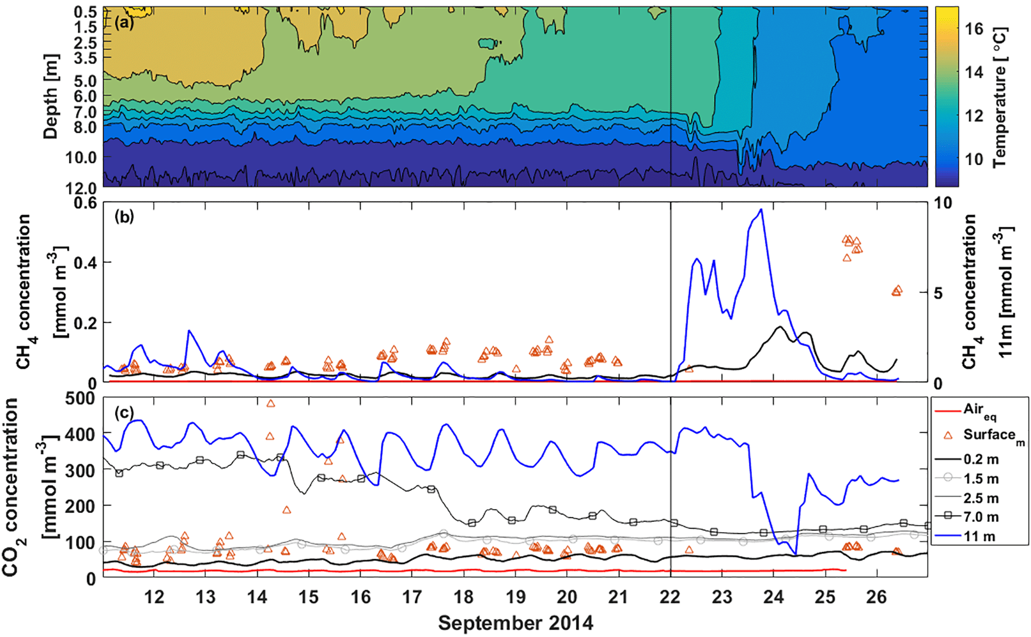
Figure 3Half-hour averages of (a) temperature, (b) CH4 concentration and (c) CO2 concentration in the water column at different depths. The red line is the equilibrium concentration of CH4 and CO2 at the surface in subplots (b) and (c), respectively. The orange triangles are manual headspace samples taken from the surface water at chamber measurement locations. Time ticks represent midnight and the vertical black line the start of the lake mixing period. Note that CH4 concentration at 11 m depth (blue line) is read from the right y axis.
All three k models are hereafter referred to as they are presented in the formulas.
The results of the measurement campaign are divided into two sub-periods (11 days of stratified period 11–21 September and 5 days of lake mixing period 22–26 September 2014) according to lake stratification and environmental conditions during the campaign, since gas transfer processes differ between these two periods. The water column started its autumn turnover on 22 September, but the mixing did not yet reach the lake bottom. Measurements of CH4 and CO2 fluxes with BLM, EC and the more sporadic FC method are first compared by examining daily median as well as daytime and night-time fluxes. Spatial variation is then studied by checking median FC fluxes in different measurement points against simultaneous EC fluxes.
3.1 Environmental conditions and water column temperature
Weather at the beginning of the measurement campaign in September 2014 was warm with a maximum air temperature of 18 ∘C (Fig. 2). Sensible and latent heat fluxes were low, less than 100 W m−2 and winds were weak, around 2 m s−1, and mostly from south. Air temperature exceeded surface water temperature during the afternoons causing negative sensible heat fluxes. Night-time air temperatures were more than 10 ∘C colder than during daytime. The lake was clearly stratified with bottom temperature around 9 ∘C, and surface water temperature about 16 ∘C (Fig. 3a). On 14 September, the mixing layer of the lake deepened from 5 m to around 6–7 m due to night-time cooling. Warm daytime air temperature then caused the surface water to stratify again. Similar occasions of night-time cooling were experienced on 16 and 17 September. The sun rose at 05:45 and set at 18:45 during the stratified period.
On 22 September, a cold front turned winds north bringing cold air and rain (11 mm on 22 September). Air temperature dropped to even 0 ∘C on 24 September and wind speeds as high as 8 m s−1 were measured at the lake. A drop in the air temperature caused a large temperature difference between air and lake surface water that together with high wind speed caused high, even 200 W m−2, positive (upward) sensible and latent heat fluxes on 22 and 23 September and a large negative (−400 W m−2) effective heat flux, resulting in a negative buoyancy flux during this cooling period. Cooling also caused the starting of the autumn mixing of Lake Kuivajärvi and the thermocline reached a depth of 8 m on 22 September. Mixing reached 11 m depth in the end of the measurement campaign on 25 September but did not yet mix the bottom waters. During the mixing period sunrise was at 06:15 and sunset at 18:15.
3.2 Water column gas concentration profiles
3.2.1 CH4 concentration profile
During the stratified period CH4 concentration according to the automatic measurements at the surface was small, only around 0.02 mmol m−3 (Fig. 3b). Manual measurements, on the other hand, show surface water concentrations of 0.07 mmol m−3 on average during the stratified period. Manual CH4 concentration measurements were always higher than automatic measurements, which might be caused by insufficient equilibration time for CH4 in the automatic measurement system or by spatial variation only caught by manual measurements. At 11 m depth CH4 concentration was almost 10 times higher than at the surface. Diel variation of CH4 concentration at 11 m could be caused by lake-side cooling and convection or, more likely, by internal waves (Stepanenko et al., 2016), triggering the lake-bottom CH4-rich sediments.
On 22 September, thermocline tilting due to high wind speed caused a rapid increase in 11 m CH4 concentration and the concentration reached its maximum of 9.6 mmol m−3 on 24 September. CH4 accumulation near the bottom usually happens in the anoxic conditions in late autumn (Stepanenko et al., 2016). CH4 concentration at 11 m depth was still three times lower than the maximum concentration found in Stepanenko et al. (2016) in late September and 2 times lower than found at 12 m depth in Miettinen et al. (2015) in September. A clear increase in CH4 surface water concentration is seen on 23 September due to upwelling and concentration up to 0.19 mmol m−3 was measured with the automatic system on 24 September. Manual measurements show concentrations up to 0.47 mmol m−3 on 25 September.
Table 1Median of all CH4 fluxes and average daytime and night-time CH4 fluxes during lake stratification and mixing periods using different measurement methods. Results of Mann–Whitney U test comparing differences between daytime and night-time fluxes are given in U test column. Note that FC fluxes are averaged also over different measurement spots. Mixing period did not include enough FC measurements for this analysis. Uncertainties are given as 25th and 75th percentiles for median fluxes and as standard errors for the flux averages.
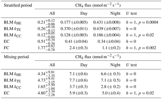

Figure 4Daily median CH4 flux from BLM, EC and FC methods. The black whiskers indicate the 25th and 75th percentiles, respectively. The vertical black line represents the start of the lake mixing period. Fluxes during (a) the stratified period (11–21 September) are read from the left and (b) mixing period fluxes (22–26 September) from the right y axis.
3.2.2 CO2 concentration profile
CO2 concentration at the surface was 47 mmol m−3 on average as measured with the automatic system during the stratified period, while manual measurements show CO2 concentration of 110 mmol m−3 at the water surface on average, similar to Miettinen et al. (2015) (Fig. 3c). On 14 September, surface layer mixing reached 7 m depth and brought CO2-rich water from deeper waters to the surface causing a drop in CO2 concentration at 7 m depth and manual samples show a rapid increase in the surface water concentration. Similar occasions on 16 and 17 September induced further decrease in CO2 concentration at 7 m depth and also an increase in the surface water CO2 concentration. After 16 September, the automatic and manual CO2 concentration measurements agree better with each other, as the average difference between the measured concentrations decreases from 114 to 16 mmol m−3. CO2 is more soluble in water than CH4 and thus equilibration time of 40 min should be enough for automatic CO2 measurements, and two different automatic systems compared well with each other on CO2 concentration at the surface (results not shown). We thereby conclude the difference between automatic and manual CO2 concentration measurements to be caused by spatial variation rather than the measurement system. We point out, however, that choosing the measurement method as well as the measurement spot has an effect on the observed concentrations and thus fluxes calculated with the BLM, as a larger concentration difference between the water surface and air would result in a larger flux in general (Eq. 2). CO2 concentration at 11 m depth was 10 times higher than at the surface and comparable to those measured in Miettinen et al. (2015) at 12 m depth. Diel variation observed in CO2 concentration at 11 m could be caused by either lake-side cooling and convection or by internal waves (Stepanenko et al., 2016).
Decreasing CO2 concentration from 390 to 63 mmol m−3 at 11 m depth observed on 23–24 September was probably due to upwelling. However, this amount of upwelling was not enough to cause a notable increase in the surface water CO2 concentration since CO2 concentration difference between the bottom and the surface is not as drastic as that of CH4, and the gas gets diluted in a large water volume on its way to the surface.
3.3 CH4 flux comparison
CH4 fluxes during the stratified period were small (less than 2 nmol m−2 s−1), estimated both with EC and BLM (Fig. 4). The EC fluxes during the stratified period were close to the detection limit (approximately 0.12 nmol m−2 s−1 for daily median flux) and are thus partly uncertain. FC fluxes were highest, reaching a maximum daily median flux of 4 nmol m−2 s−1 on 12 September. The median of all FC CH4 flux measurements during the stratified period still remained at 1.77 nmol m−2 s−1 (where the lower and upper limits represent the 25th and 75th percentiles, respectively, Table 1). Median CH4 flux according to all three methods during the stratified period was considerably lower than 4 nmol m−2 s−1 reported in Miettinen et al. (2015), who used BLM with k calculated from FC measurements, for Lake Kuivajärvi in autumn 2011 and 2012.
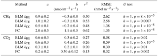
Table 2Linear fit parameters for comparison between EC and BLM fluxes according to different models for k, and between EC and FC, when EC flux estimates were on the x axis. Uncertainties are given by the standard errors of the parameters. The last column gives the results of Mann–Whitney U test for each method compared with EC. The comparison was made using daily median fluxes.
During the stratified period, EC and BLM with kTE model show no statistical difference between daytime and night-time fluxes, whereas BLM fluxes measured with kHE and kCC are slightly higher during night-time than daytime (Table 1). As the CH4 concentration difference (Δ[CH4]) between the surface water and air is lower in night-time than daytime, higher night-time fluxes are caused by gas transport coefficients kHE and kCC giving highest values at night-time (Fig. A1). The differences between daytime and night-time fluxes still remain lower than 0.3 nmol m−2 s−1. FC fluxes, however, are higher during daytime, when the concentration difference also has its maximum value.
After the mixing started on 22 September, daily median CH4 fluxes increased rapidly from 1.5 to even 15 nmol m−2 s−1 in one day due to effective mixing and gas transport from deeper waters to the surface. This increase is clearly visible in both EC and BLM fluxes, although BLM flux calculated with kCC remains lower than other BLM fluxes and is closest to EC median flux on 23 September. The flux peak in the beginning of the mixing period was over 2-fold higher compared to the 6 nmol m−2 s−1 reported in Miettinen et al. (2015), probably due to rougher weather conditions during our field campaign. Ojala et al. (2011), on the other hand, report high CH4 emissions (6 nmol m−2 s−1) after heavy rain events. Rain on 22 September could have also played a role here, enhancing the lateral transport from the catchment to the lake (Ojala et al., 2011; Rantakari and Kortelainen, 2005). However, in comparison to the situation described by Ojala et al. (2011), the rain episode in Lake Kuivajärvi was very short in duration.
During the mixing period, EC measurements show a diurnal pattern in CH4 flux with higher daytime than night-time fluxes, as was found in Keller and Stallard (1994), Bastviken et al. (2004) and Bastviken et al. (2010). BLM measurements do not show a statistical difference between daytime and night-time (Table 1). Higher daytime fluxes are expected due to higher wind speed and enhanced shear during the afternoon (Bastviken et al., 2010) as well as upwelling of CH4 from deeper layer (Fig. A2d). We find a lower concentration difference, Δ[CH4], during night-time. This may be caused by higher oxidation rate in dark, which lowers CH4 concentration in the water, and thus also the concentration difference (Dumestre et al., 1999; Mitchell et al., 2005). During daytime solar radiation, the oxidation rate would then be lower, resulting in an increase in water CH4 concentration towards the afternoon. Another possible explanation for larger concentration difference Δ[CH4] in the afternoon, in addition to CH4 feeding from the deeper waters and lower oxidation rate, is enhanced resuspension from the sediments in the littoral zone during periods of high wind speed (Bussmann, 2005). EC and BLM fluxes by kHE and kTE are also similar in magnitude (5.9 ± 0.3, 7.1 ± 0.6 and 7.7 ± 0.6 nmol m−2 s−1 daytime averages, respectively), whereas kCC gives clearly lower fluxes (3.7 ± 0.3 nmol m−2 s−1 daytime average, Table 1). Keller and Stallard (1994), Bastviken et al. (2004) and Bastviken et al. (2010) also report highest daytime fluxes for CH4 probably caused by more effective turbulent transfer during daytime, while Podgrajsek et al. (2014b) report higher night-time fluxes and suggest it to be caused by water-side convection. However, we find that both surface water concentration changes and more effective daytime gas transfer are likely explanations to the higher daytime CH4 fluxes in Lake Kuivajärvi.

Figure 5Median (a) CH4 and (b) CO2 FC fluxes (grey bars) at different measurement spots and median of simultaneous EC measurements (blue bars) during lake stratification. Black whiskers represent the 25th and 75th percentiles.
Linear fit parameters for the EC and BLM flux comparison for CH4 show that kTE (r2=0.53) and kHE (r2=0.50) were comparable to EC measurements, but kCC (r2=0.48) resulted in clearly lower fluxes than EC measurements (p<0.05, Table 2). Ebullition is not an important gas transport mechanism in the EC footprint area as found in Stepanenko et al. (2016) and thus BLM including only diffusive gas flux is expected to give results close to EC. A similar result with kCC giving the lowest flux estimate was also found in Schubert et al. (2012), where EC and FC methods gave 8 and 7 times higher cumulative fluxes than BLM with kCC. Also, Blees et al. (2015) report seasonal changes in CH4 flux due to cooling and changes in buoyancy flux. This further encourages to prefer up-to-date k models instead of kCC in CH4 flux estimates. FC measured daily median CH4 fluxes 2 times higher than EC (p<0.05, Table 2), as was also observed in Eugster et al. (2011), and thus gave highest flux estimates from all three methods. A reason behind the result might be that these low fluxes are very difficult to detect with the EC method, since the CH4 fluxes were very close to the detection limit of the EC measurement system. Higher fluxes during the mixing period could have been more suitable for a comparison between the two methods. Podgrajsek et al. (2014a) did not find systematically higher fluxes with EC or FC and found quite good agreement between these two methods for CH4 fluxes. The EC method has a larger source area (flux footprint) than FC method, which might also affect the flux. Windy conditions during the mixing period could have made the comparison better, but manual FC measurements are difficult to do during high wind and rough weather conditions.
In addition to comparison between FC and EC measurements on a temporal scale, spatial variation of CH4 flux within the EC footprint area was also studied with floating chambers at different parts of the lake during the stratified period 11–21 September 2014. The measurement spots were chosen upwind from the measurement raft to ensure being within the EC footprint area. Results are shown in Fig. 5, where the median of FC measurements at different spots are compared with the median of simultaneous EC measurements.
Measurement points N3 and N4 showed slightly higher median FC CH4 fluxes than elsewhere, although the 25th and 75th percentiles fall within the same range in all locations (Fig. 5a). Since the two measurement locations are of different depth and other locations measure similar fluxes compared to each other, we cannot make any conclusions about depth or wind direction dependencies. EC measurements do not show any difference in CH4 fluxes measured from the south side or the north side of the measurement raft. FC measured CH4 fluxes were systematically higher than simultaneous EC fluxes, independent from the measurement location.
3.4 CO2 flux comparison
CO2 flux was small (below 1 µmol m−2 s−1) at the beginning of the measurement campaign and similar to those reported in Miettinen et al. (2015), Mammarella et al. (2015) and Heiskanen et al. (2014) due to low wind speeds and thermal stratification of the lake (Fig. 6). Negative daily median EC fluxes on 11, 12 and 14 September were not statistically different from zero (p<0.05, tested with Mann–Whitney U test) and denote very small fluxes close to the detection limit of the measurement system (0.12 µmol m−2 s−1), rather than uptake, which would be very unlikely in September in a boreal lake.
Table 3Median of all CO2 fluxes and average daytime and night-time CO2 fluxes during lake stratification and mixing periods using different measurement methods. Results of Mann–Whitney U test comparing differences between daytime and night-time fluxes are given in U test column. Note that FC fluxes are averaged also over different measurement spots. Mixing period did not include enough FC measurements for this analysis. Uncertainties are given as 25th and 75th percentiles for median fluxes and as standard errors for the flux averages.
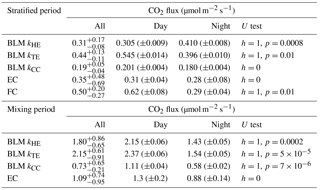
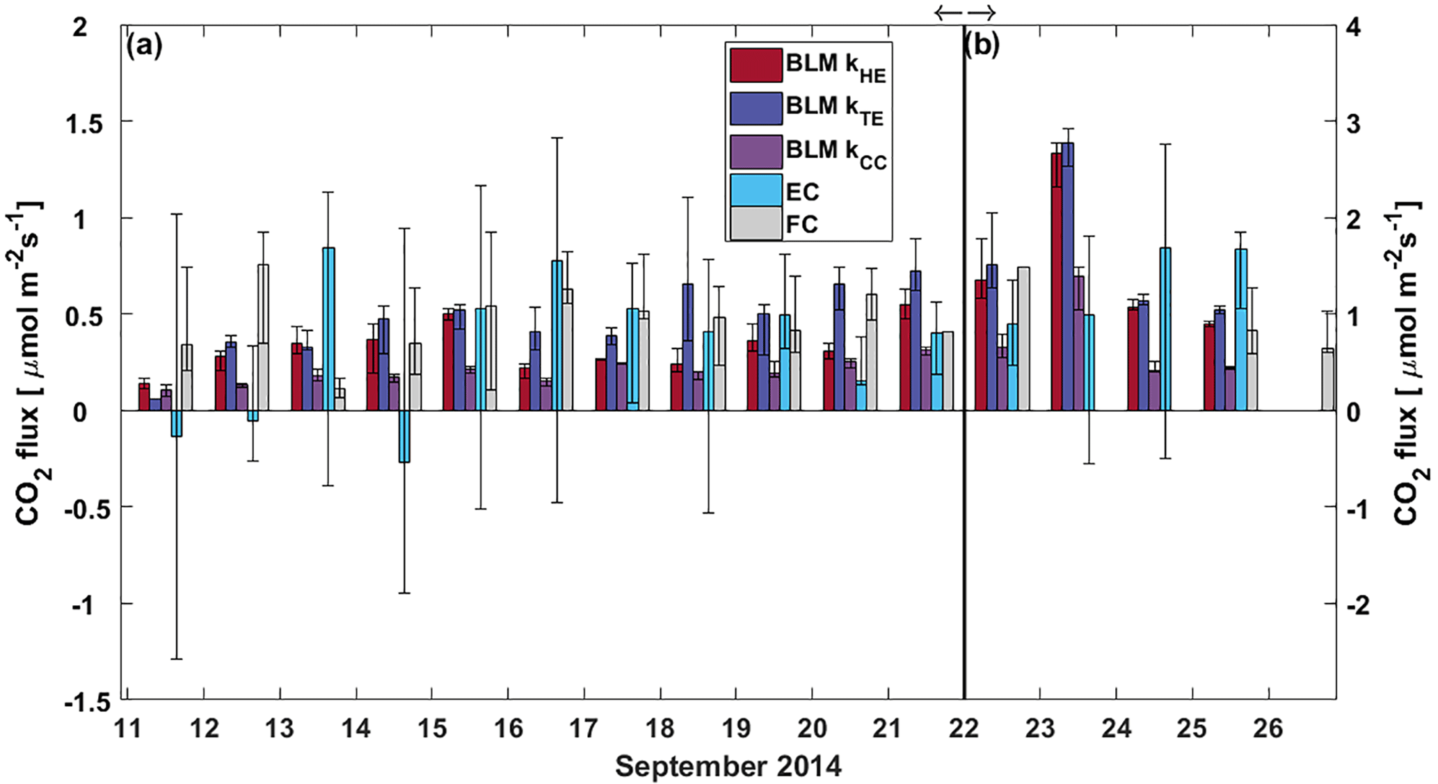
Figure 6Daily median CO2 flux from BLM, EC and FC methods. The black whiskers indicate the 25th and 75th percentiles, respectively. The vertical black line represents the start of the lake mixing period. Fluxes during (a) the stratified period (11–21 September) are read from the left and (b) mixing period fluxes (22–26 September) from the right y axis.
In the stratified period, BLM with kTE and FC methods results in a similar diurnal pattern with higher fluxes detected during daytime than night-time, while BLM with kTE shows the opposite and EC and BLM with kCC show no statistical difference between daytime and night-time fluxes (Table 3). Low BLM flux in the daytime (0.305 ± 0.009 µmol m−2 s−1 on average with kHE model) is probably caused by photosynthetic activity of algae in the lake that reduces the CO2 concentration difference between air and water (Δ[CO2]) right after sunrise (Fig. A1d, Table 3). Also, the convective term (C2w*) in kHE is zero during daytime, when the lake is heating due to higher air temperature, resulting in a lower kHE (Fig. A1a). Higher flux during night-time (0.410±0.008 on average with kHE model) is probably caused by turbulence created by waterside cooling (Heiskanen et al., 2014). This is seen in Fig. A1a as the convective term C2w* increases towards night-time causing higher gas transfer coefficient kHE and thus higher flux as well. Podgrajsek et al. (2015) argued that the main driver for enhanced night-time gas exchange is convection, and they did not find a correlation with the concentration difference Δ[CO2]. However, we find that Δ[CO2] also increases during night-time due to the absence of algal photosynthesis. BLM by kTE gives highest fluxes at noon, when friction velocity also gains its maximum value (Fig. A1c), even though Δ[CO2] is at its minimum. In the absence of buoyancy term in daytime, the gas transfer velocity kTE is solely composed of the shear term. The BLM flux by kTE is thus also larger in the daytime (0.545 ± 0.014 µmol m−2 s−1 on average, Table 3) despite the lower Δ[CO2], and night-time flux (0.396 ± 0.010 µmol m−2 s−1) is 27 % smaller than the daytime flux during the stratified period. Water friction velocity, that was used in kTE, was calculated from direct EC measurements in the air (Eq. 6). Friction velocity calculated from wind speed measurements (with a drag coefficient 0.001 for a water surface) instead of direct u*a measurements gave similar diurnal variation to model kHE (data not shown) but resulted in a lower u*w than with direct u*a measurements. BLM with kTE could give better results with direct turbulence measurements in the water. The buoyancy term (β) in kTE is low compared to the shear term () even during night-time (Fig. A1c). EC and BLM with kCC methods do not show any diurnal variation for CO2 exchange over the lake when the lake is stratified. Vesala et al. (2006) did not detect diurnal variation in CO2 EC flux in September either over a small humic lake in Finland with fluxes usually under 1 µmol m−2 s−1 during the stratified period. Overall, kHE and EC measurements agree well on the magnitude of CO2 flux during daytime, while FC measured CO2 fluxes closest to EC during night-time in the stratified period.
The flux increased almost 3-fold when the lake started mixing with higher wind speeds and was larger (3 µmol m−2 s−1) than reported in other studies from Lake Kuivajärvi (less than 2 µmol m−2 s−1; Miettinen et al., 2015; Mammarella et al., 2015). EC, on the other hand, measured daily median CO2 flux less than 2 µmol m−2 s−1, as reported in other studies.
Average daytime CO2 fluxes were 1.3 ± 0.2, 2.15 ± 0.06, 2.37 ± 0.06 and 1.11 ± 0.04 µmol m−2 s−1 with the EC method and BLM by kHE, kTE and kCC, respectively. Night-time average fluxes were notably smaller, as 0.88 ± 0.14, 1.43 ± 0.05, 1.54 ± 0.05 and 0.58 ± 0.02 µmol m−2 s−1 with the EC method and BLM by kHE, kTE and kCC, respectively (Table 3). Highest flux according to BLM with all three k models was measured at noon, when wind speeds are highest. Shear terms C1U and in kHE and kTE models, respectively, have diurnal variations with highest values at noon as well (Fig. A2a and c), which results in higher daytime BLM fluxes with kHE and kTE. BLM by kCC, however, shows considerably lower fluxes than kHE and kTE both during daytime and night-time on average. Higher fluxes during daytime than night-time in the mixing period are expected due to enhanced gas transfer during stronger winds in the daytime. The buoyancy term β in kTE is still almost a magnitude smaller than the shear term and does not influence the kTE much, even during lake mixing (Fig. A2c). The maximum and minimum concentration differences Δ[CO2] were 1.4 to 1.6 times higher during the mixing period than in the stratified period. This may be caused by upwelling of CO2 from deep waters to the surface during the mixing period and more effective algal photosynthesis during the stratified period. This indicates that selectively using only daytime gas concentration measurements in BLMs systematically biases the estimates of the long-term carbon budget.
Linear fit parameters for the comparison of BLM and FC methods with EC measurements show that kTE (r2=0.26) and kHE (r2=0.27) give the best results when compared with EC (60 % of the measured EC flux). BLM CO2 flux based on kCC was clearly underestimated, being only about 30 % of the measured EC flux (r2=0.20) and FC fluxes were also generally lower than EC (20 %, r2=0.13, Table 2). The same result of kCC giving lower fluxes than EC was found also in other studies (e.g. Heiskanen et al., 2014; Mammarella et al., 2015; Podgrajsek et al., 2015) and the use of this model in global carbon budget estimates may therefore be questionable (e.g. Raymond et al., 2013). During lake stratification, kCC gives the general flux level quite well, while during lake mixing and rain events it is clearly lower than the other measured fluxes. However, on an annual scale, these special occasions might contribute significantly to the CH4 and CO2 budgets (Miettinen et al., 2015; Ojala et al., 2011; Podgrajsek et al., 2014a) and should be noted in upscaled flux estimates.
During the stratified period, CO2 fluxes were almost always higher when measured with FC than simultaneous EC measurements, as also found in Eugster et al. (2003) and Podgrajsek et al. (2014a) (statistical significance tested with Mann–Whitney U test, p<0.05), although daily median values were, on average, higher when measured with EC than FC (Table 2). Lower daily median FC fluxes might thus result from discontinuous FC measurements missing important episodic flux events, as suggested by Podgrajsek et al. (2014a). However, from the north side of the measurement raft (measurement spots N1–N4), FC fluxes do not differ statistically from EC CO2 fluxes.
The FC measurements did not show spatial variation in CO2 flux but there is a clear difference between EC measurements from the south and north sides of the lake (tested with Mann–Whitney U test, p<0.05) with approximately 0.1 µmol m−2 s−1 higher CO2 fluxes measured from the south than from north (Fig. 5b). The south side of the raft is shallower than the north side (Fig. 1a) and thus more prone for the mixing to reach bottom even during the stratified period. The EC footprint area of 100–300 m (Mammarella et al., 2015) from the raft reaches further to the shallow areas than the FC measurements that were done approximately 50 m south from the raft. EC is thus more likely to catch the higher gas fluxes resulting from upwelling of gas-rich waters from the bottom. Higher CH4 flux from the south side was not detected possibly due to CH4 oxidation in the water column into CO2. This oxidation would not increase the CO2 efflux, as CH4 flux is so much smaller than that of CO2. The footprint area north from the raft is over significantly deeper water and mixing from the deeper waters during stratified period is unlikely.
We found that all gas transfer velocity, k, models used in BLM calculation gave mainly lower flux estimates of both CH4 and CO2 compared to EC, while FC measurements were mostly higher than EC. For CH4 fluxes, this difference between the FC and EC methods is probably caused by the fact that, during lake stratification, the measured fluxes were very small, close to the detection limit of the EC system. For CO2, there was no statistical difference between the FC and EC methods over the north side of the lake, and night-time average fluxes were almost the same with these two methods. Gas transfer velocity models by Tedford et al. (2014) (kTE) and Heiskanen et al. (2014) (kHE) showed very similar fluxes both for CH4 and CO2, and the k model by Cole and Caraco (1998) (kCC) resulted in clearly lower gas fluxes especially during the lake mixing period. A comparison between BLM and EC fluxes showed that, on average, the kTE model is the most similar and the kCC model the lowest, when compared to EC fluxes. For global upscaling, it would be preferable to use up-to-date k models instead of kCC to reduce the risk of systematic biases. The simple kCC model underestimates the flux especially during special occasions of, for example, lake mixing and rain events, which may vastly contribute to the annual flux estimate.
During the stratified period, CO2 flux by kTE showed higher daytime than night-time fluxes, opposite to other models, due to higher air friction velocity during daytime. This model could work better with direct friction velocity measurements in the water. The buoyancy term included in kTE model was not significant compared to the shear term even in night-time, and does not affect the diurnal variation of the flux. CO2 concentration difference between the surface water and air was found to have a diurnal cycle with lower values during daytime, probably due to algal photosynthesis reducing surface water concentration of CO2. An opposite diurnal cycle was found for CH4 concentration difference with highest values reached in the afternoon. This might be due to CH4 feeding from the deeper waters, lower oxidation rate in daylight in the water column, or more effective lateral transport from the littoral zone during higher wind speeds in the daytime. As we observe a clear diurnal cycle in the concentration difference for both CH4 and CO2, it is important to note that using only daytime concentration (and wind speed) measurements for upscaling with BLM affects the resulting flux estimate.
Including the effect of lake cooling clearly improves the flux estimate both for CH4 and CO2, although these models are not as simple to use as wind-speed-based models. In the absence of an extensive measurement system, the use of e.g. bulk formulas for estimating latent and sensible heat fluxes for kHE and kTE would result in better flux estimates than the use of kCC. This would require an estimate for the depth of the actively mixing layer, light extinction coefficient, radiation data, and wind speed, as well as temperature and moisture differences between the air and water surface. With this information, it is possible to calculate the effective heat flux and buoyancy flux, after which estimating kHE and kTE is straightforward, keeping in mind that the water-side friction velocity for kTE model may be estimated from wind speed measurements by scaling it with an appropriate drag coefficient.
FC measurements did not show a spatial variation in either CH4 or CO2 flux. CO2 EC flux was clearly higher from the south side of the measurement raft than north, due to the shallower lake area within the EC footprint on the south side. This was not detected with CH4, possibly due to oxidation in the water column.
FC measurements are generally used for studying spatial variation, but our results suggest that EC measurements are also able to detect differences between different wind sectors. EC measurement systems are set up in one place, often on the shore or on a raft near the deepest parts of the lake to have a large footprint area for measurements. This is due to one of the limitations in the EC method, because it requires a homogeneous surface and favourable wind conditions but leads to possibly biased flux estimations, especially if flux is only measured over a particularly deep or shallow area not representative of the lake. The FC method is good for detecting spatial variation but has its limitations regarding temporal and spatial data coverage and challenging measurements in windy and wavy weather conditions. As we find clear differences between night-time and daytime flux measurements as well as between stratified and lake mixing periods, it is advisable to prefer frequent and diverse sampling over daytime-only measurements, which can lead to biases in greenhouse gas budget estimates.
Eddy covariance, water column temperature and CO2 concentration and meteorological data are available in the AVAA – Open research data publishing platform (http://openscience.fi/avaa). The metadata of the observations are available via the ETSIN service. Data from manual measurements are available upon request from the first author.
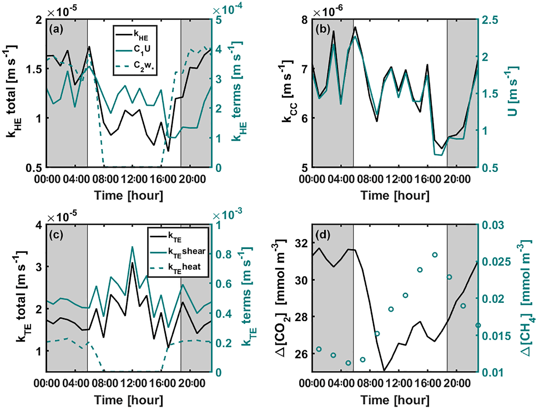
Figure A1Diurnal variation of (a) kHE and its shear and convective terms (Eq. 9), (b) kCC and wind speed, (c) kTE and its shear ( or ) and convective ( or kTEheat=0) terms (Eq. 8), and (d) CO2 and CH4 concentration differences between air and surface water during the stratified period 11–21 September 2014. Shear and convective terms in subplots (a) and (c) are not corrected with the Schmidt number. Grey areas represent night-time.
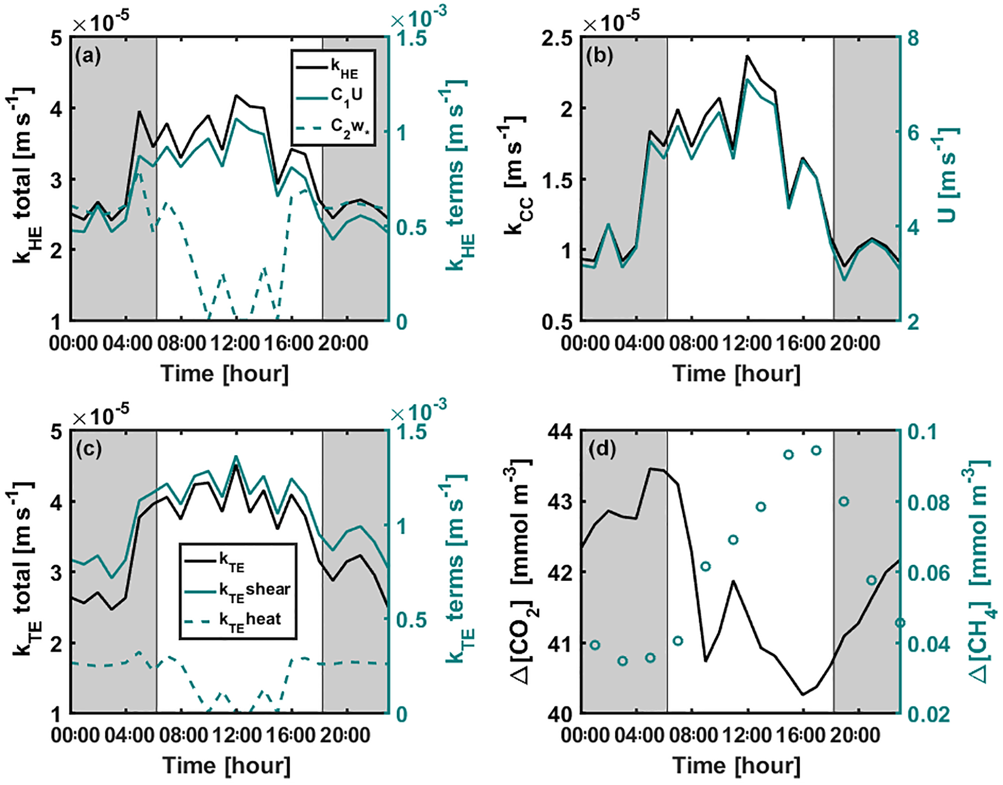
Figure A2Diurnal variation of (a) kHE and its shear and convective terms (Eq. 9), (b) kCC and wind speed, (c) kTE and its shear ( or ) and convective ( or kTEheat=0) terms (Eq. 8), and (d) CO2 and CH4 concentration differences between air and surface water during the mixing period 22–26 September 2014. Shear and convective terms in subplots (a) and (c) are not corrected with the Schmidt number. Grey areas represent night-time.
IM, DB, JH, MR and TV designed the field experiments. KME, MR, AO and JH carried out manual field measurements. KME, IM and OP participated in eddy covariance data processing and analysis. TB and AL carried out automatic gas concentration measurements in the water column. All authors participated in analysing the results, and KME and IM prepared the manuscript with contributions from all co-authors.
The authors declare that they have no conflict of interest.
We thank the Hyytiälä Forestry Field Station staff for all their technical
support and Maria Gutierrez de los Rios for her help during the measurement
campaign. This study was supported by EU project GHG-LAKE (612642), Academy
of Finland (CarLAC (281196) project, Centre of Excellence (272041), Academy
Professor projects (284701 and 282842)), SRC-VR and ERC 725546 and
ICOS-FINLAND (281255).
Edited by: Gwenaël Abril
Reviewed by: two anonymous referees
Aubinet, M., Vesala, T., and Papale, D. (Eds.): Eddy covariance: a practical guide to measurement and data analysis, Springer Science & Business Media, 2012. a
Bastviken, D., Cole, J., Pace, M., and Tranvik, L.: Methane emissions from lakes: Dependence of lake characteristics, two regional assessments, and a global estimate, Global Biogeoch. Cy., 18, GB4009, https://doi.org/10.1029/2004GB002238, 2004. a, b
Bastviken, D., Santoro, A. L., Marotta, H., Pinho, L. Q., Calheiros, D. F., Crill, P., and Enrich-Prast, A.: Methane emissions from Pantanal, South America, during the low water season: toward more comprehensive sampling, Environ. Sci. Technol., 44, 5450–5455, 2010. a, b, c
Bastviken, D., Tranvik, L. J., Downing, J. A., Crill, P. M., and Enrich-Prast, A.: Freshwater methane emissions offset the continental carbon sink, Science, 331, 50–50, 2011. a
Blees, J., Niemann, H., Erne, M., Zopfi, J., Schubert, C. J., and Lehmann, M. F.: Spatial variations in surface water methane super-saturation and emission in Lake Lugano, southern Switzerland, Aquat. Sci., 77, 535–545, https://doi.org/10.1007/s00027-015-0401-z, 2015. a
Bussmann, I.: Methane release through resuspension of littoral sediment, Biogeochemistry, 74, 283–302, https://doi.org/10.1007/s10533-004-2223-2, 2005. a
Cole, J. J. and Caraco, N. F.: Atmospheric exchange of carbon dioxide in a low-wind oligotrophic lake measured by the addition of SF6, Limnol. Oceanogr., 43, 647–656, 1998. a, b, c, d, e
Cole, J. J., Caraco, N. F., Kling, G. W., and Kratz, T. K.: Carbon dioxide supersaturation in the surface waters of lakes, Science (New York, N.Y.), 265, 1568–1570, 1994. a
Cole, J. J., Prairie, Y. T., Caraco, N. F., McDowell, W. H., Tranvik, L. J., Striegl, R. G., Duarte, C. M., Kortelainen, P., Downing, J. A., and Middelburg, J. J.: Plumbing the global carbon cycle: integrating inland waters into the terrestrial carbon budget, Ecosystems, 10, 172–185, 2007. a
Duc, N. T., Silverstein, S., Lundmark, L., Reyier, H., Crill, P., and Bastviken, D.: Automated flux chamber for investigating gas flux at water–air interfaces, Environ. Sci. Technol., 47, 968–975, 2013. a
Dumestre, J. F., Guézennec, J., Galy-Lacaux, C., Delmas, R., Richard, S., and Labroue, L.: Influence of light intensity on methanotrophic bacterial activity in Petit Saut Reservoir, French Guiana, Appl. Environ. Microbiol., 65, 534–539, 1999. a
Eugster, W., Kling, G., Jonas, T., McFadden, J. P., Wüest, A., MacIntyre, S., and Chapin, F. S.: CO2 exchange between air and water in an Arctic Alaskan and midlatitude Swiss lake: Importance of convective mixing, J. Geophys. Res.-Atmos. (1984–2012), 108, 4362, https://doi.org/10.1029/2002JD002653, 2003. a
Eugster, W., DelSontro, T., and Sobek, S.: Eddy covariance flux measurements confirm extreme CH4 emissions from a Swiss hydropower reservoir and resolve their short-term variability, Biogeosciences, 8, 2815–2831, https://doi.org/10.5194/bg-8-2815-2011, 2011. a
Finkelstein, P. L. and Sims, P. F.: Sampling error in eddy correlation flux measurements, J. Geophys. Res.-Atmos., 106, 3503–3509, 2001. a
Gålfalk, M., Bastviken, D., Fredriksson, S., and Arneborg, L.: Determination of the piston velocity for water-air interfaces using flux chambers, acoustic Doppler velocimetry, and IR imaging of the water surface, J. Geophys. Res.-Biogeosci., 118, 770–782, https://doi.org/10.1002/jgrg.20064, 2013. a, b
Hari, P. and Kulmala, M.: Station for Measuring Ecosystem–Atmosphere Relations (SMEAR II), Boreal Environ. Res., 10, 315–322, 2005. a
Hari, P., Pumpanen, J., Huotari, J., Kolari, P., Grace, J., Vesala, T., and Ojala, A.: High-frequency measurements of productivity of planktonic algae using rugged nondispersive infrared carbon dioxide probes, Limnol. Oceanogr., 6, 347–354, 2008. a
Heiskanen, J. J., Mammarella, I., Haapanala, S., Pumpanen, J., Vesala, T., MacIntyre, S., and Ojala, A.: Effects of cooling and internal wave motions on gas transfer coefficients in a boreal lake, Tellus B, 66, 22827, https://doi.org/10.3402/tellusb.v66.22827, 2014. a, b, c, d, e, f, g, h, i
Heiskanen, J. J., Mammarella, I., Ojala, A., Stepanenko, V., Erkkilä, K.-M., Miettinen, H., Sandström, H., Eugster, W., Leppäranta, M., Järvinen, H., Vesala, T., and Nordbo, A.: Effects of water clarity on lake stratification and lake-atmosphere heat exchange, J. Geophys. Res.-Atmos., 120, 7412–7428, https://doi.org/10.1002/2014JD022938, 2015. a, b
Huotari, J., Ojala, A., Peltomaa, E., Nordbo, A., Launiainen, S., Pumpanen, J., Rasilo, T., Hari, P., and Vesala, T.: Long term direct CO2 flux measurements over a boreal lake: Five years of eddy covariance data, Geophys. Res. Lett., 38, L18401, https://doi.org/10.1029/2011GL048753, 2011. a
Imberger, J.: The diurnal mixed layer, Limnol. Oceanogr., 30, 737–770, 1985. a
Keller, M. and Stallard, R. F.: Methane emission by bubbling from Gatun Lake, Panama, J. Geophys. Res.-Atmos., 99, 8307–8319, https://doi.org/10.1029/92JD02170, 1994. a, b
Lehner, B. and Döll, P.: Development and validation of a global database of lakes, reservoirs and wetlands, J. Hydrol., 296, 1–22, https://doi.org/10.1016/j.jhydrol.2004.03.028, 2004. a
Liu, H., Peters, G., and Foken, T.: New equations for sonic temperature variance and buoyancy heat flux with an omnidirectional sonic anemometer, Bound.-Lay. Meteorol., 100, 459–468, https://doi.org/10.1175/JHM-D-12-020.1, 2001. a
Livingston, G. P. and Hutchinson, G. L.: Enclosure-based measurement of trace gas exchange: applications and sources of error, in: Biogenic trace gases: measuring emissions from soil and water, edited by: Matson, P. and Harriss, R., 14–51, Blackwell Science Ltd, 1995. a
Lorke, A., Bodmer, P., Noss, C., Alshboul, Z., Koschorreck, M., Somlai-Haase, C., Bastviken, D., Flury, S., McGinnis, D. F., Maeck, A., Müller, D., and Premke, K.: Technical note: drifting versus anchored flux chambers for measuring greenhouse gas emissions from running waters, Biogeosciences, 12, 7013–7024, https://doi.org/10.5194/bg-12-7013-2015, 2015. a, b
MacIntyre, S., Wanninkhof, R., and Chanton, J. P.: Trace gas exchange across the air-water interface in freshwater and coastal marine environments, in: Biogenic trace gases: measuring emissions from soil and water, edited by: Matson, P. and Harriss, R., 52–97, Blackwell Science Ltd, 1995. a
Mammarella, I., Launiainen, S., Grönholm, T., Keronen, P., Pumpanen, J., Rannik, Ü., and Vesala, T.: Relative humidity effect on the high-frequency attenuation of water vapor flux measured by a closed-path eddy covariance system, J. Atmos. Ocean. Tech., 26, 1856–1866, https://doi.org/10.1175/2009JTECHA1179.1, 2009. a
Mammarella, I., Nordbo, A., Rannik, Ü., Haapanala, S., Levula, J., Laakso, H., Ojala, A., Peltola, O., Heiskanen, J., Pumpanen, J., and Vesala, T.: Carbon dioxide and energy fluxes over a small boreal lake in Southern Finland, J. Geophys. Res.-Biogeosci., 120, 1296–1314, https://doi.org/10.1002/2014JG002873, 2015. a, b, c, d, e, f, g, h, i, j, k, l, m
Mammarella, I., Peltola, O., Nordbo, A., Järvi, L., and Rannik, Ü.: Quantifying the uncertainty of eddy covariance fluxes due to the use of different software packages and combinations of processing steps in two contrasting ecosystems, Atmos. Meas. Tech., 9, 4915–4933, https://doi.org/10.5194/amt-9-4915-2016, 2016. a
Miettinen, H., Pumpanen, J., Heiskanen, J. J., H., A., Mammarella, I., Ojala, A., Levula, J., and Rantakari, M.: Towards a more comprehensive understanding of lacustrine greenhouse gas dynamics – two-year measurements of concentrations and fluxes of CO2, CH4 and N2O in a typical boreal lake surrounded by managed forests, Boreal Environ. Res., 20, 75–89, 2015. a, b, c, d, e, f, g, h, i
Mitchell, B. G., Broody, E. A., Holm-Hansen, O., and McClain, C.: Inhibitory effect of light on methane oxidation in the pelagic water column of a mesotrophic lake (Lake Biwa, Japan), Limnol. Oceanogr, 36, 1662–1677, 2005. a
Natchimuthu, S., Sundgren, I., Gålfalk, M., Klemedtsson, L., Crill, P., Danielsson, Å., and Bastviken, D.: Spatio-temporal variability of lake CH4 fluxes and its influence on annual whole lake emission estimates, Limnol. Oceanogr., 61, S13–S26, https://doi.org/10.1002/lno.10222, 2016. a
Ojala, A., Lopez Bellido, J., Tulonen, T., Kankaala, P., and Huotari, J.: Carbon gas fluxes from a brown-water and a clear-water lake in the boreal zone during a summer with extreme rain events, Limnol. Oceanogr., 56, 61–76, https://doi.org/10.4319/lo.2011.56.1.0061, 2011. a, b, c
Podgrajsek, E., Sahlée, E., Bastviken, D., Holst, J., Lindroth, A., Tranvik, L., and Rutgersson, A.: Comparison of floating chamber and eddy covariance measurements of lake greenhouse gas fluxes, Biogeosciences, 11, 4225–4233, https://doi.org/10.5194/bg-11-4225-2014, 2014a. a, b, c, d
Podgrajsek, E., Sahlée, E., and Rutgersson, A.: Diurnal cycle of lake methane flux, J. Geophys. Res.-Biogeosci., 119, 236–248, https://doi.org/10.1002/2013JG002327, 2014b. a
Podgrajsek, E., Sahlée, E., and Rutgersson, A.: Diel cycle of lake-air CO2 flux from a shallow lake and the impact of waterside convection on the transfer velocity, J. Geophys. Res.-Biogeosci., 120, 29–38, https://doi.org/10.1002/2014JG002781, 2015. a, b
Rannik, Ü., Peltola, O., and Mammarella, I.: Random uncertainties of flux measurements by the eddy covariance technique, Atmos. Meas. Tech., 9, 5163–5181, https://doi.org/10.5194/amt-9-5163-2016, 2016. a
Rantakari, M. and Kortelainen, P.: Interannual variation and climatic regulation of the CO2 emission from large boreal lakes, Glob. Change Biol., 11, 1368–1380, 2005. a
Raymond, P. A., Hartmann, J., Lauerwald, R., Sobek, S., McDonald, C., Hoover, M., Butman, D., Striegl, R., Mayorga, E., and Humborg, C.: Global carbon dioxide emissions from inland waters, Nature, 503, 355–359, https://doi.org/10.1038/nature12760, 2013. a, b
Schubert, C. J., Diem, T., and Eugster, W.: Methane emissions from a small wind shielded lake determined by eddy covariance, flux chambers, anchored funnels, and boundary model calculations: a comparison, Environ. Sci. Technol., 46, 4515–4522, 2012. a, b, c
Seinfeld, J. H. and Pandis, S. N.: Atmospheric chemistry and physics: from air pollution to climate change, John Wiley & Sons, 2016. a
Stepanenko, V., Mammarella, I., Ojala, A., Miettinen, H., Lykosov, V., and Vesala, T.: LAKE 2.0: a model for temperature, methane, carbon dioxide and oxygen dynamics in lakes, Geosci. Model Dev., 9, 1977–2006, https://doi.org/10.5194/gmd-9-1977-2016, 2016. a, b, c, d, e
Tedford, E. W., MacIntyre, S., Miller, S. D., and Czikowsky, M. J.: Similarity scaling of turbulence in a temperate lake during fall cooling, J. Geophys. Res.-Oceans, 119, 4689–4713, https://doi.org/10.1002/2014JC010135, 2014. a, b, c, d, e
Tranvik, L. J., Downing, J. A., Cotner, J. B., Loiselle, S. A., Striegl, R. G., Ballatore, T. J., Dillon, P., Finlay, K., Fortino, K., and Knoll, L. B.: Lakes and reservoirs as regulators of carbon cycling and climate, Limnol. Oceanogr., 54, 2298–2314, https://doi.org/10.4319/lo.2009.54.6_part_2.2298, 2009. a
Verpoorter, C., Kutser, T., Seekell, D. A., and Tranvik, L. J.: A global inventory of lakes based on high-resolution satellite imagery, Geophys. Res. Lett., 41, 6396–6402, https://doi.org/10.1002/2014GL060641, 2014. a
Vesala, T., Huotari, J., Rannik, U., Suni, T., Smolander, S., Sogachev, A., Launiainen, S., and Ojala, A.: Eddy covariance measurements of carbon exchange and latent and sensible heat fluxes over a boreal lake for a full open water period, J. Geophys. Res.-Atmos., 111, https://doi.org/10.1029/2005JD006365, 2006. a
Vickers, D. and Mahrt, L.: Quality control and flux sampling problems for tower and aircraft data, J. Atmos. Ocean. Tech., 14, 512–526, 1997. a
Warneck, P. and Williams, J.: The atmospheric Chemist’s companion: numerical data for use in the atmospheric sciences, Springer Science & Business Media, 2012. a