Technical Note: An efficient method for accelerating the spin-up process for process-based biogeochemistry models

Qu, Yang; Maksyutov, Shamil; Zhuang, Qianlai

doi:https://doi.org/10.5194/bg-15-3967-2018

Articles | Volume 15, issue 13

https://doi.org/10.5194/bg-15-3967-2018

Articles | Volume 15, issue 13

Technical note

03 Jul 2018

Technical note |

| 03 Jul 2018

Technical Note: An efficient method for accelerating the spin-up process for process-based biogeochemistry models

Yang Qu, Shamil Maksyutov, and Qianlai Zhuang

Abstract

To better understand the role of terrestrial ecosystems in the global carbon cycle and their feedbacks to the global climate system, process-based biogeochemistry models need to be improved with respect to model parameterization and model structure. To achieve these improvements, the spin-up time for those differential equation-based models needs to be shortened. Here, an algorithm for a fast spin-up was developed by finding the exact solution of a linearized system representing the cyclo-stationary state of a model and implemented in a biogeochemistry model, the Terrestrial Ecosystem Model (TEM). With the new spin-up algorithm, we showed that the model reached a steady state in less than 10 years of computing time, while the original method requires more than 200 years on average of model run. For the test sites with five different plant functional types, the new method saves over 90 % of the original spin-up time in site-level simulations. In North American simulations, average spin-up time savings for all grid cells is 85 % for either the daily or monthly version of TEM. The developed spin-up method shall be used for future quantification of carbon dynamics at fine spatial and temporal scales.

Download & links

Article (PDF, 1133 KB)

How to cite

How to cite.

Dates

Received: 20 Feb 2018 – Discussion started: 12 Mar 2018 – Revised: 05 Jun 2018 – Accepted: 11 Jun 2018 – Published: 03 Jul 2018

1 Introduction

Biogeochemistry models contain state variables representing various pools of carbon and nitrogen and a set of flux variables representing the element and material transfers among different state variables. Model spin-up is a step to get biogeochemistry models to a steady state for those state and flux variables (McGuire et al., 1992; King, 1995; Johns et al., 1997; Dickinson et al., 1998). Spin-up normally uses cyclic forcing data to force the model run and reach a steady state, which will be used as initial conditions for model transient simulations. The steady state is reached when modeled state variables show a cyclic pattern or a constant value and often requires a significant amount of computation time, which needs to be accelerated for regional and global simulations at fine spatial and temporal scales.

Spin-up is normally achieved by running the model repeatedly using one or several decades of meteorological or climatic data until a steady state is reached. The step could require that the model repeatedly run for more than 2000 annual cycles in some extreme cases. Specifically, the model will check the stability of the simulated carbon and nitrogen fluxes as well as state variables with specified threshold values. For instance, the model will check if the simulated annual net ecosystem production (NEP) is less than 1 g C m⁻² yr⁻¹ (McGuire et al., 1992). Another method to reach a steady state is to obtain the analytical solutions (King et al., 1995; Comins, 1997), which might also take a significantly long time.

For different biogeochemistry models, spin-up could take hundreds and thousands of years to reach a stability, normally longer than the model projection period (Thornton and Rosenbloom, 2005). Therefore, a more efficient method to reach the steady state will speed up the entire model simulation. Recently, a semi-analytical method (Xia et al., 2012) has been adapted to a carbon–nitrogen coupled model to speed up the spin-up process. The idea is to obtain an analytical solution very close to a steady condition, then start spin-up from the solution, which could significantly reduce spin-up time. This technique did not reach a cyclic pattern for state and flux variables and required an additional spin-up process to achieve the steady state. However, Lardy et al. (2011) and Martin et al. (2007) have implemented their spin-up methods for a linear problem of soil carbon dynamics including their seasonal cycles.

Here we developed a method to accelerate the spin-up process in a nonlinear model. We tested the method for representative PFTs and North America with both daily and monthly versions of the Terrestrial Ecosystem Model (TEM; Zhuang et al., 2003). In addition, we compared the performance of our algorithms with the semi-analytical version of Xia et al. (2012). The new algorithms will help us conduct very high spatial and temporal resolution simulations with process-based biogeochemistry models in the future.

2 Method

2.1 TEM description

We used a process-based biogeochemistry model, TEM (Zhuang et al., 2003), as a test bed to demonstrate the performance of the new algorithms of spin-up. TEM simulates the dynamics of ecosystem carbon and nitrogen fluxes and pools (McGuire et al., 1992; Zhuang et al., 2010, 2003). It contains five state variables: carbon in living vegetation (C_v), nitrogen in living vegetation (N_v), organic carbon in detritus and soils (C_s), organic nitrogen in detritus and soils (N_s), and available inorganic soil nitrogen (N_av). Carbon and nitrogen dynamics in TEM are governed by the following equations:

\begin{array}{l} (1) & \frac{d C_{v}}{d t} = GPP - R_{A} - L_{C}, \\ (2) & \frac{d N_{v}}{d t} = NUPTAKE - L_{N}, \\ (3) & \frac{d C_{s}}{d t} = L_{c} - R_{H}, \\ (4) & \frac{d N_{s}}{d t} = L_{N} - NETNMIN, \\ (5) & \frac{d N_{av}}{d t} = NINPUT + NETNMIN - NLOST - NUPTAKE, \end{array}

where GPP is gross primary production, R_A is autotrophic respiration, L_Cis carbon in litterfall, NUPTAKE is nitrogen uptake by vegetation, L_N is nitrogen in litterfall, R_H is heterotrophic respiration, NETNMIN is net rate of mineralization of soil nitrogen, NINPUT is nitrogen input from the outside ecosystem, and NLOST is nitrogen loss from the ecosystem. Key carbon fluxes are defined as

\begin{array}{l} GPP = C_{max} f (PAR) f (PHENOLOGY) f (FOLIAGE) \\ (6) & f (T) f (C_{a}, G_{v}) f (NA) f (FT), \\ (7) & NPP = GPP - R_{A}, \\ (8) & NEP = GPP - R_{A} - R_{H} . \end{array}

For detailed GPP definition, see Zhuang et al. (2003). NEP will be near zero when the ecosystem reaches a steady state. Therefore, the spin-up goal is to keep running the model driven with repeated climate forcing data until NEP is close to zero with a certain tolerance value (e.g., 0.1 g C m⁻² yr⁻¹).

2.2 Spin-up acceleration method

TEM can be reformulated as

\begin{matrix} (9) & \frac{d x}{d t} = g (x, t) + h (t), \end{matrix}

where x is a vector of state variables (e.g., C_V); h(t) is the vector of carbon–nitrogen input from the atmosphere (such as nitrogen input), independent of x; and g(x,t) is the process rate function of element pools (e.g., GPP).

By linearizing the model in terms of pools, we could obtain

\begin{matrix} (10) & g (x, t) = g (x_{0}, t) + J (x - x_{0}), \end{matrix}

where x₀ is initial pool sizes and J is the Jacobian matrix of the process rate:

\begin{matrix} (11) & J = \frac{d g}{d x} = (\begin{array}{ccc} \frac{\partial g_{1}}{\partial x_{1}} & \dots & \frac{\partial g_{1}}{\partial x_{n}} \\ ⋮ & ⋮ \\ \frac{\partial g_{n}}{\partial x_{1}} & \dots & \frac{\partial g_{n}}{\partial x_{n}} \end{array}), \end{matrix}

where g represents g(x,t). x_n represents each state variable in the TEM (e.g., V_C). The numerical discretization of Eq. (9) is

\begin{array}{l} x_{i, k} - x_{i, k - 1} = τ \cdot J_{k - \frac{1}{2}} \cdot x_{i, k - 1} \\ (12) & + τ (g (x_{0}, k - 1) - J_{k - \frac{1}{2}} \cdot x_{0, k - 1} + h_{k - 1}), \end{array}

where τ is time step (month), x_i, k is the pool x_i size at time k, and J_k−½ is a Jacobian matrix at time step $k - \frac{1}{2}$ . Here $\frac{1}{2}$ refers to the half time step in the middle of a month, at which values of J are calculated as the mean value at time steps k and k−1. x_i,0 refers to the initial pool x_i size.

We introduce

\begin{matrix} (13) & f_{k - 1} = g (x_{0}, k - 1) - J_{k - \frac{1}{2}} \cdot x_{0, k - 1} + h_{k - 1} . \end{matrix}

The Eq. (12) can then be written as

\begin{matrix} (14) & x_{i, k} - x_{i, k - 1} = τ \cdot J_{k - \frac{1}{2}} \cdot x_{i, k - 1} + τ \cdot f_{k - 1}, \end{matrix}

where J_k−½ is a Jacobian matrix at the time step $k - \frac{1}{2}$ . After running a large number of annual cycles, the model approaches a cyclo-stationary state, which can be expressed by condition $x_{T + i} = x_{i}$ , where T is the number of time steps in one cycle, for example, when spin-up is made at a monthly time step using monthly climatology of temperature, precipitation and other forcing data, T=12, and $\vec{x_{1}}$ is the size of carbon pools on 1 January, while J^1.5 is the matrix of mean process rate constants for January.

By introducing

A_{k} = τ \cdot J_{k - \frac{1}{2}}, y_{k} = τ f_{k - 1}, B_{k} = I, C_{k} = I + A,

where I is an identity matrix, Eq. (12) can be further written as

\begin{matrix} (15) & - C_{k} \cdot x_{i, k - 1} + B_{k} \cdot x_{i, k} = y_{k} . \end{matrix}

The cyclic boundary condition is $x_{1} = x_{T + 1}$ .

Then Eq. (13) will become

\begin{matrix} (15a) & - C_{1} \cdot x_{i, T} + B_{1} \cdot x_{i, 1} = y_{1} . \end{matrix}

Thus Eq. (15) and (15a) become a formulation of a linear problem with T unknown vectors $\vec{x_{T}}$ , which can be solved using LU (lower and upper) decomposition or Gaussian elimination (Martin et al., 2007). Xia et al. (2012; see Eq. 4) and Kwon and Primeau (2006) also had linear equations for a steady state, but conducted the model simulation at an annual time step. Going for annual average form reduces the size of the problem and prevents Xia et al. (2012) from obtaining the exact solution of the problem including seasonal cycle (see their Eqs. 15, 15a). While our new approach runs the model at a monthly time step with the cyclic boundary conditions for state variables x, it still targets a steady state for the ecosystem at an annual time step instead of a monthly time step.

2.3 Numerical implementation

Equation (15a) is explicitly expressed as

\begin{array}{l} (\begin{array}{cccccccc} B & 0 & 0 & \dots & 0 & 0 & 0 & - C \\ - C & B & 0 & \dots & 0 & 0 & 0 & 0 \\ 0 & - C & B & \dots & 0 & 0 & 0 & 0 \\ \dots & \dots & \dots & \dots & \dots & \dots & \dots & \dots \\ 0 & 0 & 0 & \dots & - C & B & 0 & 0 \\ 0 & 0 & 0 & \dots & 0 & - C & B & 0 \\ 0 & 0 & 0 & \dots & 0 & 0 & - C & B \end{array}) \\ (16) & \times (\begin{array}{c} x_{1} \\ x_{2} \\ \cdot \\ \cdot \\ \cdot \\ \cdot \\ x_{T} \end{array}) = (\begin{array}{c} y_{1} \\ y_{2} \\ \cdot \\ \cdot \\ \cdot \\ \cdot \\ y_{T} \end{array}) . \end{array}

Equation (16) can be shown in the form Mx=Y.

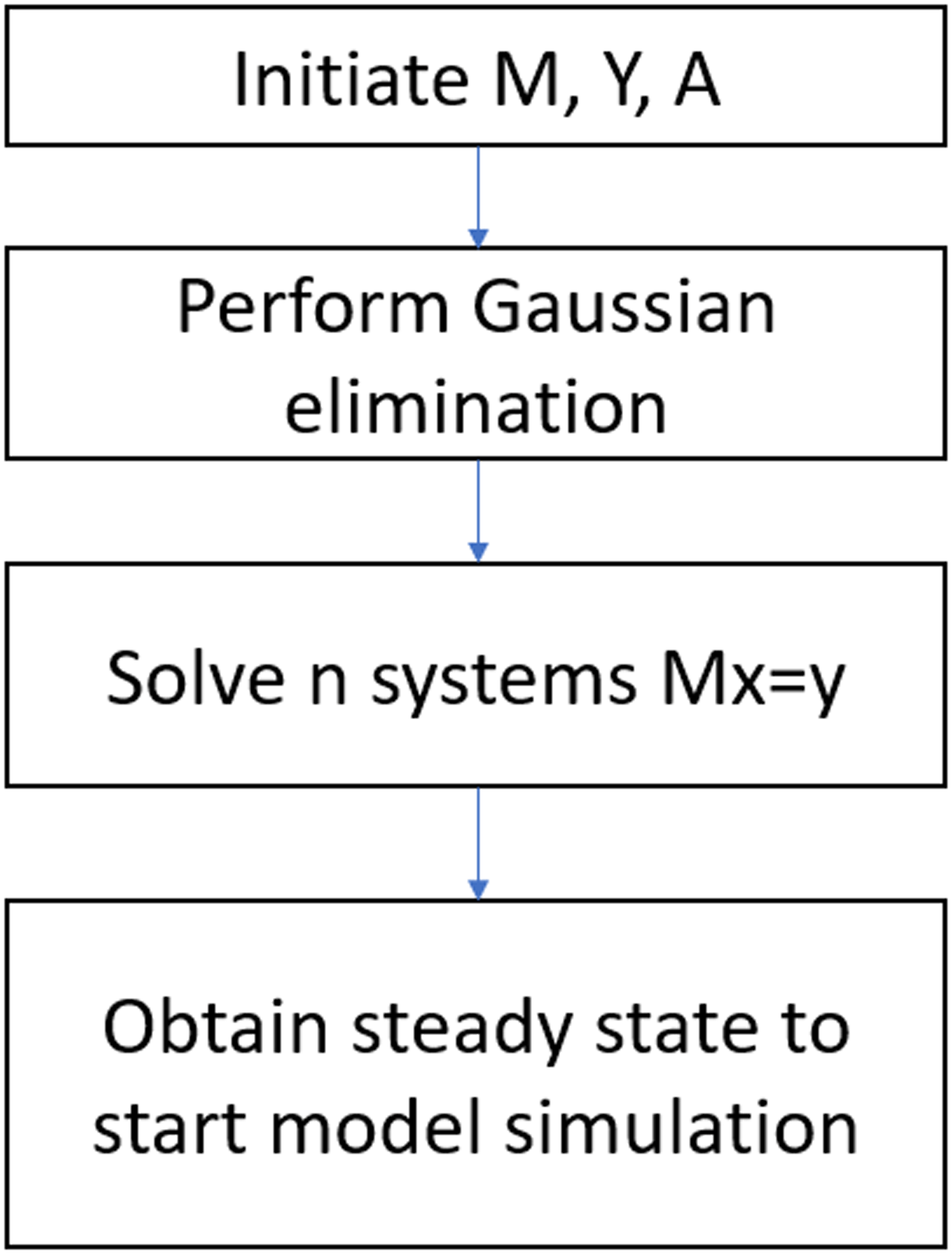
We apply the Gaussian elimination to the upper block that reduces M to a lower triangular form (Fig. 1). The resulting matrix is lower diagonal:

\begin{matrix} (17) & M^{'} = (\begin{array}{cccccccc} B^{'} & 0 & 0 & \dots & 0 & 0 & 0 & 0 \\ - C & B & 0 & \dots & 0 & 0 & 0 & 0 \\ 0 & - C & B & \dots & 0 & 0 & 0 & 0 \\ \dots & \dots & \dots & \dots & \dots & \dots & \dots & \dots \\ 0 & 0 & 0 & \dots & - C & B & 0 & 0 \\ 0 & 0 & 0 & \dots & 0 & - C & B & 0 \\ 0 & 0 & 0 & \dots & 0 & 0 & - C & B \end{array}) . \end{matrix}

Equation (16) is thus reduced to the form $M^{'} x = Y^{'}$ , where M^′ is the lower diagonal, and solution of Eqs. (15a) and (16) will be readily obtained for x.

https://www.biogeosciences.net/15/3967/2018/bg-15-3967-2018-f01

Figure 1Algorithms and procedures of the new spin-up method.

Download

2.4 Algorithm implementation for TEM

In the original TEM, carbon fluxes can be defined as

\begin{array}{l} (18) & NPP = GPP - MR - GR, \\ (19) & MR = V_{C} \cdot K_{T}, \\ (20) & GR = \{\begin{cases} 0.25 \cdot (GPP - MR), & if GPP > MR \\ 0, & otherwise \end{cases}, \end{array}

where NPP is defined as the difference of GPP and plant maintenance respiration (MR) and growth respiration (GR). MR is assumed as a function of C_V and temperature (K_T). Here we revised MR calculation:

\begin{array}{l} MR \\ (21) & = \{\begin{cases} V_{C} \cdot K_{T}, & if GPP > V_{C} \cdot K_{T} \\ 0.75 \cdot V_{C} \cdot K_{T} + 0.25 \cdot GPP, & otherwise . \end{cases} \end{array}

Table 1Test sites for new spin-up algorithms.

Download Print Version | Download XLSX

https://www.biogeosciences.net/15/3967/2018/bg-15-3967-2018-f02

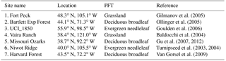
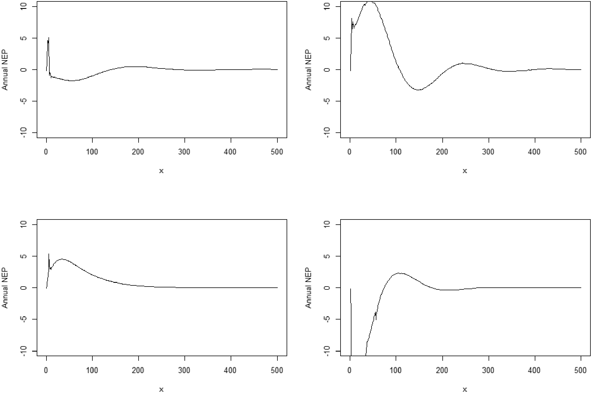
Figure 2The time for NEP (g C yr⁻¹ m⁻²) to reach a steady state with the original spin-up method at the Harvard Forest site. x represents model simulation years.

Download

The NEP is defined as the difference between NPP and heterotrophic respiration (R_H).

The basic workflow to implement the method is (1) linearizing TEM first to obtain a sparse matrix with n variable (for TEM, n = 5) system, (2) performing Gaussian elimination for the linear system and (3) solving the sparse matrix to acquire the state variable values (Fig. 1). To adapt this method to a daily version of TEM, we changed the cyclic condition T from 12 to 365. The other steps are the same as for the monthly version. We tested the new method for the carbon-only version and carbon–nitrogen coupled version of TEM for different PFTs (Table 1). Specifically, for the carbon-only version, we only solved the differential equations that govern the carbon dynamics, while for the carbon–nitrogen coupled version, we solved the differential equations that govern both carbon and nitrogen dynamics in the system. For both versions, the spin-up process strives to reach a steady state for carbon pools and fluxes.

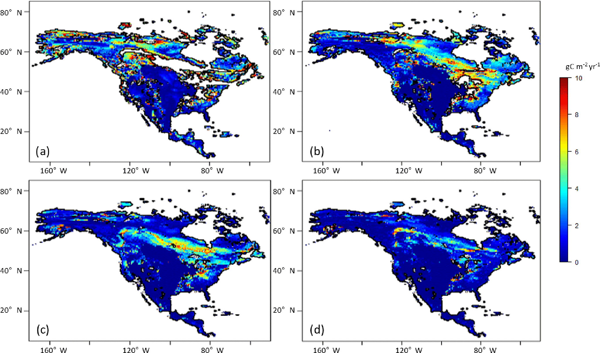
https://www.biogeosciences.net/15/3967/2018/bg-15-3967-2018-f03

Figure 3Simulated NEP (g C m⁻² yr⁻¹) with the original spin-up method after different spin-up times of (a) 50, (b) 100, (c) 150 and (d) 200 years. After these spin-up times, 63, 89, 93 and 98 % of grids reach their steady states, respectively.

Download

3 Results and discussion

At the Harvard Forest site, the traditional spin-up method took 564 years to reach the steady state for both the carbon-only and coupled carbon–nitrogen simulations with an annual NEP of less than 0.1 g C m⁻² yr⁻¹ (Fig. 2). In contrast, the improved method took 72 years for the carbon only and 122 for the coupled carbon–nitrogen simulations. For carbon and nitrogen pools, it took another 45 years (equivalent cyclic time) to reach a steady state with a NEP of less than 0.1 g C m⁻² yr⁻¹. In comparison with the traditional spin-up method (Zhuang et al., 2003), the new method saved 65 % of computational time to reach the steady state in the carbon-only simulations (Table 2). The differences in steady-state carbon pools between using the new method and traditional spin-up methods were small (less than 0.85 %). Similarly, for the coupled carbon–nitrogen simulations, the new method saves a similar amount of time to reach the steady state.

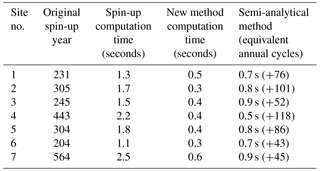
For all seven test sites, the original spin-up method in TEM takes 204–564 years (1.1–2.5 s of computing time) to reach the steady state at different sites. In contrast, our new method only takes 0.3–0.6 s, while the semi-analytical method (Xia et al., 2012) will need 0.5–0.9 s to reach the steady state at different sites (Table 2). Compared to the original spin-up method, the new method is not only faster but also computationally stable.

The time of spin-up to reach a steady state of NEP varied for different PFT grids using the original method (Fig. 2). In general, to allow 98 % of grid cells to reach their steady states of NEP, it takes 250 annual model runs, while the new method will only need on average of 0.6 s (equivalent to 60-year annual model runs with the original method) (Fig. 3). For regional tests in North America, we found that the average saving time with the new method with monthly TEM is 25, 32 and 22 % for Alaska, Canada and the conterminous US, respectively.

Table 2Spin-up time comparison for different methods for seven study sites; seconds represent real computation time, and years refer to the annual spin-up cycles.

Download Print Version | Download XLSX

To compare the performance of the new method with other existing methods, we adapted the semi-analytical method (Xia et al., 2012) to the TEM model. To do that, we first revised the TEM model structure to

\begin{matrix} (22) & \frac{d P (t)}{d t} = ε AC P (t), \end{matrix}

where P(t) is a vector of pools in TEM (e.g., C_V and C_S). ε is a scalar. A is a pool transfer matrix (in which A_ij represents the fraction of carbon transfer from pool j to i). C is a diagonal matrix with pool components (where diagonal components quantify the fraction of carbon left from the state variables after each time step). With this method, we obtained an analytical solution for the intermediate state. We then kept running TEM with the traditional spin-up process. Specifically, we started TEM simulation to estimate the state variable values. Based on these values, the spin-up runs were conducted to reach the final steady state. We found that the semi-analytical solution is better than the original spin-up method but slower than the new method proposed in this study (Table 2).

The TEM model has a relatively small set of state variables for carbon and nitrogen. The version we used is TEM 5.0, which has only five state variables (Zhuang et al., 2003). Thus, the linearization process is relatively easy and the matrix size is relatively small; consequently, the computing is not a burden. To accelerate the spin-up for multiple soil carbon pool models with relatively simple and linear decomposition processes, implementing our method will still be relatively easy but will take a great amount of computing time to equilibrate. For models such as CLM, multiple methods have been tested to accelerate their spin-up process (e.g., Fang et al., 2015), the direct analytical solution method introduced in this study might be time consuming to achieve.

4 Summary

We developed a new method to speed up the spin-up process in process-based biogeochemistry models. We found that the new method shortened 90 % of the spin-up time using the traditional method. For regional simulations in North America, average spin-up time saving is 85 % for either daily or monthly version of TEM. We consider our method is a general approach to accelerate the spin-up process for process-based biogeochemistry models. As long as the governing equations of the models can be formulated as the form in Eq. (9), the algorithm could be adopted accordingly. Our method will significantly help future carbon dynamics quantification with biogeochemistry models at fine spatial and temporal scales.

Data availability

All data used in this study are available from the authors upon request.

Author contributions

QZ and SM designed and supervised the research. YQ performed model simulations and data analysis. All authors contributed to the paper writing.

Competing interests

The authors declare that they have no conflict of interest.

Acknowledgements

This study is supported through projects funding to Qianlai Zhuang from the Department of Energy (DESC0008092 and DE-SC0007007) and the NSF Division of Information and Intelligent Systems (NSF-1028291). The supercomputing resource is provided by the Rosen Center for Advanced Computing at Purdue University.

Edited by: Christopher A. Williams
Reviewed by: two anonymous referees

References

Baldocchi, D. D., Xu, L., and Kiang, N.: How plant functional-type, weather, seasonal drought, and soil physical properties alter water and energy fluxes of an oak–grass savanna and an annual grassland, Agr. Forest Meteorol., 123, 13–39, 2004.

Comins, H. N.: Analysis of nutrient-cycling dynamics, for predicting sustainability and CO₂-response of nutrient-limited forest ecosystems, Ecol. Model., 99, 51–69, 1997.

Dickinson, R. E., Shaikh, M., Bryant, R., and Graumlich, L.: Interactive canopies for a climate model, J. Climate, 11, 2823–2836, 1998.

Fang, Y., Liu, C., and Leung, L. R.: Accelerating the spin-up of the coupled carbon and nitrogen cycle model in CLM4, Geosci. Model Dev., 8, 781–789, https://doi.org/10.5194/gmd-8-781-2015, 2015.

Gilmanov, T. G., Demment, M. W., Wylie, B. K., Laca, E. A., Akshalov, K., Baldocchi, D. D., and Emmerich, W. E.: Quantification of the CO₂ exchange in grassland ecosystems of the world using tower measurements, modeling and remote sensing, in: XX International Grassland Congress: offered papers, 26, p. 587, 2005

Goulden, M. L., Winston, G. C., McMillan, A. M. S., Litvak, M. E., Read, E. L., Rocha, A. V., and Rob Elliot, J.: An eddy covariance mesonet to measure the effect of forest age on land–atmosphere exchange, Glob. Change Biol., 12, 2146–2162, 2006.

Gu, L., Meyers, T., Pallardy, S. G., Hanson, P. J., Yang, B., Heuer, M., and Wullschleger, S. D.: Influences of biomass heat and biochemical energy storages on the land surface fluxes and radiative temperature, J. Geophys. Res.-Atmos., 112, https://doi.org/10.1029/2006JD007425, 2007.

Gu, L., Massman, W. J., Leuning, R., Pallardy, S. G., Meyers, T., Hanson, P. J., and Yang, B.: The fundamental equation of eddy covariance and its application in flux measurements, 152, 135-148, Agr. Forest Meteorol., 2012.

Johns, T. C., Carnell, R. E., Crossley, J. F., Gregory, J. M., Mitchell, J. F., Senior, C. A., Tett, S. F. B., and Wood, R. A.: The second Hadley Centre coupled ocean-atmosphere GCM: model description, spinup and validation, Clim. Dynam., 13, 103–134, 1997.

King, D. A.: Equilibrium analysis of a decomposition and yield model applied to Pinus radiata plantations on sites of contrasting fertility, Ecol. Model., 83, 349–358, 1995.

Kwon, E. Y. and Primeau, F.: Optimization and sensitivity study of a biogeochemistry ocean model using an implicit solver and in situ phosphate data, Global Biogeochem. Cy., 20, GB4009, https://doi.org/10.1029/2005GB002631, 2006.

Lardy, R., Bellocchi, G., and Soussana, J. F.: A new method to determine soil organic carbon equilibrium, Environ. Modell. Softw., 26, 1759–1763, 2011.

Martin, M. P., Cordier, S., Balesdent, J., and Arrouays, D.: Periodic solutions for soil carbon dynamics equilibriums with time-varying forcing variables, Ecol. Model., 204, 523–530, 2007.

McGuire, A. D., Melillo, J. M., Joyce, L. A., Kicklighter, D. W., Grace, A. L., Moore, B. I. I. I., and Vorosmarty, C. J.: Interactions between carbon and nitrogen dynamics in estimating net primary productivity for potential vegetation in North America, Global Biogeochem. Cy., 6, 101–124, 1992.

NVIDIA CUDA Compute Unified Device Architecture Programming Guide, NVIDIA Corporation, 2007.

Ollinger, S. V. and Smith, M. L.: Net primary production and canopy nitrogen in a temperate forest landscape: an analysis using imaging spectroscopy, modeling and field data, Ecosystems, 8, 760–778, 2005.

Thornton, P. E. and Rosenbloom, N. A.: Ecosystem model spin-up: Estimating steady state conditions in a coupled terrestrial carbon and nitrogen cycle model, Ecol. Model., 189, 25–48, 2005.

Turnipseed, A. A., Anderson, D. E., Blanken, P. D., Baugh, W. M., and Monson, R. K.: Airflows and turbulent flux measurements in mountainous terrain: Part 1. Canopy and local effects, Agr. Forest Meteorol., 119, 1–21, 2003.

Turnipseed, A. A., Anderson, D. E., Burns, S., Blanken, P. D., and Monson, R. K.: Airflows and turbulent flux measurements in mountainous terrain: Part 2: Mesoscale effects, Agr. Forest Meteorol., 125, 187–205, 2004.

Van Gorsel, E., Delpierre, N., Leuning, R., Black, A., Munger, J. W., Wofsy, S., and Chen, B.: Estimating nocturnal ecosystem respiration from the vertical turbulent flux and change in storage of CO₂, Agr. Forest Meteorol., 149(11), 1919–1930, 2009.

Xia, J. Y., Luo, Y. Q., Wang, Y.-P., Weng, E. S., and Hararuk, O.: A semi-analytical solution to accelerate spin-up of a coupled carbon and nitrogen land model to steady state, Geosci. Model Dev., 5, 1259–1271, https://doi.org/10.5194/gmd-5-1259-2012, 2012.

Zhuang, Q., McGuire, A. D., Melillo, J. M., Clein, J. S., Dargaville, R. J., Kicklighter, D. W., Myneni, R. B., Dong, J., Romanovsky, V. E., Harden, J., and Hobbie, J. E.: Carbon cycling in extratropical terrestrial ecosystems of the Northern Hemisphere during the 20th century: a modeling analysis of the influences of soil thermal dynamics, Tellus B, 55, 751–776, 2003.

Zhuang, Q., He, J., Lu, Y., Ji, L., Xiao, J., and Luo, T.: Carbon dynamics of terrestrial ecosystems on the Tibetan Plateau during the 20th century: an analysis with a process-based biogeochemical model, Global Ecol. Biogeogr., 19, 649–662, 2010.

Articles

Short summary

We developed an algorithm for a fast spin-up by finding the exact solution of a linearized system representing the cyclo-stationary state of a model and implemented it in a biogeochemistry model, the Terrestrial Ecosystem Model. For the test sites with five different plant functional types, the new method saves over 90 % of the original spin-up time in site-level simulations. The developed spin-up method will be used for future quantification of carbon dynamics at fine spatiotemporal scales.