the Creative Commons Attribution 4.0 License.
the Creative Commons Attribution 4.0 License.
 | 14 Jun 2018
Sea-surface dimethylsulfide (DMS) concentration from satellite data at global and regional scales
Maurice Levasseur
Emmanuel Devred
Rafel Simó
Marcel Babin
The marine biogenic gas dimethylsulfide (DMS) modulates climate by enhancing aerosol light scattering and seeding cloud formation. However, the lack of time- and space-resolved estimates of DMS concentration and emission hampers the assessment of its climatic effects. Here we present DMSSAT, a new remote sensing algorithm that relies on macroecological relationships between DMS, its phytoplanktonic precursor dimethylsulfoniopropionate (DMSPt) and plankton light exposure. In the first step, planktonic DMSPt is estimated from satellite-retrieved chlorophyll a and the light penetration regime as described in a previous study (Galí et al., 2015). In the second step, DMS is estimated as a function of DMSPt and photosynthetically available radiation (PAR) at the sea surface with an equation of the form: . The two-step DMSSAT algorithm is computationally light and can be optimized for global and regional scales. Validation at the global scale indicates that DMSSAT has better skill than previous algorithms and reproduces the main climatological features of DMS seasonality across contrasting biomes. The main shortcomings of the global-scale optimized algorithm are related to (i) regional biases in remotely sensed chlorophyll (which cause underestimation of DMS in the Southern Ocean) and (ii) the inability to reproduce high DMS ∕ DMSPt ratios in late summer and fall in specific regions (which suggests the need to account for additional DMS drivers). Our work also highlights the shortcomings of interpolated DMS climatologies, caused by sparse and biased in situ sampling. Time series derived from MODIS-Aqua in the subpolar North Atlantic between 2003 and 2016 show wide interannual variability in the magnitude and timing of the annual DMS peak(s), demonstrating the need to move beyond the classical climatological view. By providing synoptic time series of DMS emission, DMSSAT can leverage atmospheric chemistry and climate models and advance our understanding of plankton–aerosol–cloud interactions in the context of global change.
- Article
(5200 KB) -
Supplement
(3578 KB) - BibTeX
- EndNote


Ocean-emitted gases and particles control the number, size distribution and composition of aerosols in remote oceanic areas (Brooks and Thornton, 2018). These aerosols scatter sunlight and can act as cloud condensation nuclei that alter the radiative properties of clouds, both microscopic (cloud droplet number concentration and effective radius) and macroscopic (cloud abundance, albedo and lifetime). Interactions between natural aerosols and clouds are a major source of uncertainty in climate projections, confounding the calculation of natural and anthropogenic radiative forcing and the attribution of anthropogenic climate change (Carslaw et al., 2013). Therefore, there is an urgent need to better understand and model the oceanic sources of aerosols, and to better resolve their variations at relevant spatial and temporal scales, from weekly to seasonal to interannual.
The gas dimethylsulfide (DMS) is produced by marine microbial food webs in the sunlit layer of the ocean. With its emission currently estimated at 28 Tg S yr−1, it contributes about 70 % of natural sulfur emissions to the global atmosphere and a major portion of the marine emission of organic volatiles (Carpenter et al., 2012; Schlesinger and Bernhardt, 2013; Simó, 2011). The cloud-seeding activity of DMS and its potential role in climate regulation were first postulated 3 decades ago (Charlson et al., 1987; Shaw, 1983). The so-called CLAW hypothesis (Charlson et al., 1987) proposed that a negative feedback could operate between marine phytoplankton, DMS emission and cloud albedo, potentially regulating the Earth's climate. Posterior research showed that the mechanisms behind the potential loop are far more complex than initially envisaged. This, and the estimated low sensitivity of each step of the feedback to changes in its forcing factors, led Quinn and Bates (2011) to refute the CLAW hypothesis.
Nevertheless, atmospheric studies powered by new analytical techniques (Kulmala et al., 2014) and modeling have shown instances where marine DMS controls ultrafine aerosol particle formation in the Arctic (Leaitch et al., 2013; Park et al., 2017), temperate North Atlantic (Sanchez et al., 2018), Antarctica (Yu and Luo, 2010) and the tropical South Pacific atmospheres (Modini et al., 2009). Moreover, Quinn et al. (2017) recently reported that DMS-derived aerosols dominate cloud condensation nuclei populations over most of the global ocean. Hence, the influence of DMS on marine stratiform cloud albedo remains in the spotlight (Brooks and Thornton, 2018), and the occurrence of a “seasonal CLAW” in remote marine atmospheres is becoming increasingly conceivable (Levasseur, 2013; Vallina and Simó, 2007a).
DMS is produced by marine microbial food webs through a complex network of biological interactions and chemical processes (Simó, 2004). Its primary source is the enzymatic cleavage of dimethylsulfoniopropionate (DMSP), a multifunctional osmolyte that accumulates at high (hundred millimolar) intracellular concentrations in some phytoplankton, especially haptophytes, dinoflagellates and some picoeukaryotes (Stefels et al., 2007). DMSP cleavage is catalyzed by a wide diversity of enzymes, called DMSP lyases, produced by some phytoplankton (Alcolombri et al., 2015) and bacteria (Curson et al., 2011). Breakage of phytoplankton cells through zooplankton grazing, viral attack and autolysis releases DMSP to the algal boundary layer and the dissolved phase and enhances DMS production (Simó, 2004; Stefels et al., 2007). Another process that contributes to DMS production is the diffusive release of DMS from phytoplankton cells, which proceeds almost instantaneously after intracellular DMSP cleavage by DMSP lyases or by photochemically produced radicals (Lavoie et al., 2015; Mopper et al., 2015). Once in seawater, DMS is removed by biotic and abiotic processes. DMS budgets in the upper mixed layer (UML) indicate that, on average, about 90 % of dissolved DMS is consumed by bacterial oxidation and UV-driven photolysis, and only 10 % is emitted to the atmosphere through turbulent diffusion (Galí and Simó, 2015).
Seawater DMS concentration controls the emission flux because the oceanic UML is largely supersaturated with respect to the atmosphere. DMS concentration in the UML is regulated by a subtle dynamic equilibrium between production and consumption processes with a typical timescale of less than 4 days (Galí and Simó, 2015). Over the seasonal cycle, DMS concentration varies mainly in response to the phenology and ecological succession of microbial species and their interplay with physical forcing factors, particularly solar exposure and nutrient supply, which are in turn regulated by vertical mixing (Galí and Simó, 2015; Lizotte et al., 2012; Simó and Pedrós-Alió, 1999). For instance, diatom blooms, typical of nutrient replete conditions at high latitudes, are characterized by low DMSP concentration per unit biomass and low DMSP-to-DMS conversion yield (Lizotte et al., 2012). The opposite is true for microbial communities typical of stratified, nutrient-depleted and highly irradiated surface waters, both at low and high latitudes (Galí and Simó, 2010; Lizotte et al., 2012). Under these conditions, two main factors act synergistically to increase DMS concentration (Galí and Simó, 2015; Vallina et al., 2008): the higher contribution of DMSP-rich species to total phytoplankton biomass (Galí et al., 2015; Stefels et al., 2007); and the higher DMSP-to-DMS conversion yield at the microbial community level, possibly caused by the effects of nutrient and irradiance stress (Galí et al., 2013; Stefels, 2000; Sunda et al., 2002, 2007; Vallina et al., 2008). As a result, similar DMS concentrations may occur in waters that differ by 1 or 2 orders of magnitude in phytoplankton biomass (Lizotte et al., 2012), and DMS tends to peak in summer across polar to tropical latitudes, lagging the annual chlorophyll peak by some months in the subtropical gyres. The mismatch between phytoplankton biomass, DMSP and DMS, termed the DMS summer paradox (Simó and Pedrós-Alió, 1999), is an essential feature that biogeochemical models strive to reproduce with mixed success (Le Clainche et al., 2010).
With nearly 50 000 DMS measurements taken between 1972 and 2010, the global sea-surface DMS database (https://saga.pmel.noaa.gov/dms/, last access: 13 April 2017) is a valuable resource for model development and validation. Gridded monthly climatologies (Kettle et al., 1999; Lana et al., 2011) calculated from this dataset are the standard DMS product used as input to atmospheric chemistry and climate models, hence emphasizing the seasonal climatological view (Mahajan et al., 2015; McCoy et al., 2015). At the other end, the climatic role of DMS is often evaluated through extreme sensitivity tests that examine the response of Earth system models to order-of-magnitude perturbations of DMS emission (e.g., Grandey and Wang, 2015). In comparison, contemporaneous decadal-scale DMS variability has received less attention. This gap can be filled using empirical remote sensing algorithms, a handful of which have been developed since the early 2000s (Tesdal et al., 2016; see also the pioneering works of Jodwalis and Benner, 1995, and Thompson et al., 1990). Interestingly, large discrepancies exist among global DMS fields estimated with interpolated climatologies, empirical algorithms or prognostic biogeochemical models (Tesdal et al., 2016). Although it is tempting to attribute these discrepancies to the poor skill of the models, they may also arise from issues in the calculation of the climatology.
Here we present DMSSAT, a new remote sensing algorithm for DMS that proceeds in two steps: (i) estimation of the concentration of the phytoplanktonic DMS precursor, total dimethylsulfoniopropionate (DMSPt), from remotely sensed chlorophyll and light penetration, and from climatological mixed layer depth (MLD); (ii) estimation of DMS concentration from DMSPt and solar irradiance. This two-step empirical algorithm reflects, with a simplified formulation, the mechanistic understanding of oceanic sulfur cycling described in the previous paragraphs. The DMSPt sub-algorithm was presented by Galí et al. (2015) and is briefly described in Appendix A. Thus, here we focus on the second step, based on the nonlinear relationship between DMS, DMSPt and photosynthetically available radiation (PAR) at the sea surface. We implement our algorithm to produce a global DMS climatology, which we compare to the latest version of the interpolated DMS climatology (Lana et al., 2011; L11 hereafter) and to climatologies derived from other remote sensing algorithms that follow similar rationales (Simó and Dachs, 2002; Vallina and Simó, 2007b). Finally, we implement our algorithm using 14 years of MODIS-Aqua satellite data in the subtropical and the subpolar North Atlantic and in the northeast Pacific to illustrate and understand interannual DMS variability.
2.1 Datasets used for algorithm development and validation
In situ concentrations of DMS and DMSPt (nM) and chlorophyll a (Chl, mg m−3), accompanied by ancillary data (bottom depth, temperature, salinity, wind speed), were downloaded from the global sea-surface DMS database. The latter was complemented with additional in situ datasets recently obtained by the authors' teams. After quality control, the database had 41 304, 3700 and 9182 measurements for in situ DMS, DMSPt and Chl, respectively, with 3637 DMS–DMSPt and 8141 DMS–Chl pairs.The in situ database was extended with geophysical and biogeochemical parameters, including satellite retrievals collocated in time and space (“matchups”) and gridded climatological datasets, following Galí et al. (2015; see below). Detailed information regarding data sources, quality control and processing can be found in the Supplement and in Tables S1–S3.
We performed satellite matchups using SeaWiFS (1997–2010) and MODIS-Aqua (2003–2012) retrievals of remotely sensed Chl (mg m−3), vertical attenuation coefficient at 490 nm (Kd490, m−1), particulate inorganic carbon (PIC, mol m−3) and daily photosynthetically available radiation at the sea surface (PAR, ). To maximize the amount of available matchups, and after verifying the consistency between the two sensors, we produced merged variables by averaging SeaWiFS and MODIS-Aqua matchups. We employed a hierarchical search procedure whereby the matchup criteria were progressively relaxed from 1 to 8 days and from single-pixel to 5×5 pixel bins (Sect. S2 in the Supplement). These merged variables are hereafter designated with the SAT subscript (e.g., ChlSAT). Daily sea-surface temperature (SSTSAT, ∘C) from the AVHRR sensors was also matched to the database.
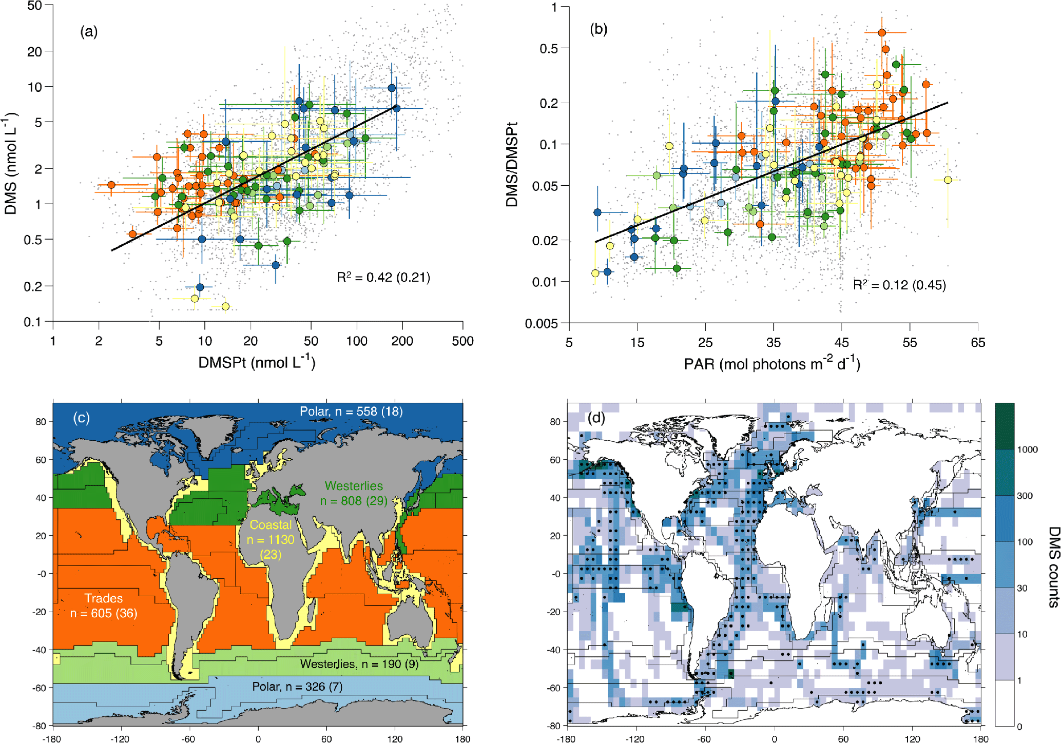
Figure 1Relationship between DMS, DMSPt and PAR across oceanic biomes and data availability. (a) DMS vs. DMSPt. (b) DMS ∕ DMSPt ratio vs. mean daily irradiance (PAR) at the sea surface. (c) Longhurst biogeochemical provinces and biomes. (d) In situ DMS data counts in latitude–longitude bins; stippling indicates bins with measurements available for 3 or more months. In (a, b) small grey dots represent individual data points and large colored dots represent the median in a given Longhurst biogeochemical province and month and the corresponding interquartile ranges. Province–month medians are colored by biome following the map in (c), which also shows the amount of DMS–DMSPt–PAR measurements available in each biome. In (a–c), the R2 and n (data counts) outside and inside parentheses correspond to non-binned data and province–month (MLongh) binned data, respectively. Regression lines in (a, b), calculated with MLongh binned data, are only illustrative.
The database was further extended with monthly climatological data: daily PAR from SeaWiFS (1997–2010 average); mixed layer depth (MLD, in meters) from the monthly MIMOC climatology (Schmidtko et al., 2013); bottom depth from the General Bathymetric Chart of the Oceans (GEBCO08); and sea-surface nitrate and phosphate concentrations (µM) from the World Ocean Atlas 2009 (WOA09). Nutricline depths were calculated from WOA09 vertical profiles as the depth where nitrate and phosphate first exceeded 1 and 0.4 µM, respectively. Nutricline depth estimations were robust to changes of ±50 % in these concentration thresholds.
The mean daily PAR in the upper mixed layer (PARMLD) was calculated as
When satellite matchups were not available (before September 1997), we used climatological PAR from SeaWiFS (1997–2010 average) in order to increase the temporal coverage of the PARSAT and PARMLD variables. Statistical analyses done with climatological or matchup PARSAT gave very similar results. This procedure was not followed with other variables (Chl, PIC, Kd490) that show wider interannual variations.
2.2 Statistical analyses and data binning schemes
All statistical analyses were conducted using (i) non-binned data; (ii) data binned by month and latitude–longitude bins (M5×5); and (iii) data binned by month and the 56 Longhurst biogeochemical provinces (designated MLongh; Longhurst, 2010). Data binning eliminates low-frequency variation (“noise”) below a given space or timescale. MLongh binned data were further aggregated into six biomes: two Polar biomes (Arctic and Antarctic), two mid-latitude Westerlies biomes (Northern and Southern hemispheres), one Trades biome (tropical latitudes) and one global Coastal biome (Fig. 1c). Variables with a right-skewed approximate lognormal distribution entered statistical analyses after log 10 transformation: DMS, DMSPt, DMS ∕ DMSPt ratio, Chl, nitrate and phosphate concentrations. To further account for non-normality, we conducted statistical explorations using both bin means and bin medians.
To develop the DMS algorithm we analyzed the relationship between DMS, the DMS ∕ DMSPt ratio and environmental variables (listed in Table 1). After an exploratory analysis based on the calculation of Pearson correlation coefficients (Table 1), we built several regression models where DMS was estimated as a function of in situ DMSPt concentration and additional variables (Tables 2 and S4). We added one variable at a time in order of decreasing data availability, and significant terms were selected using stepwise regression with entrance and removal p values set at 0.001 and 0.005, respectively. The logic for adding one variable at a time, rather than building a single initial model with all the predictor variables, is that the size (N) of the data subset used for model fitting decreases rapidly when variables with sparse coverage are combined. Each set of initial predictors was tested across the three degrees of data binning described above and three degrees of model complexity: linear without interactions, linear with interactions and quadratic with interactions. This 3×3 nested structure provided a stringent test for the robustness of a given regression model. Improvements in model performance were assessed based on the increase in adjusted r squared, , and the decrease in root-mean-square error (RMSE) and the Akaike information criterion (AIC).
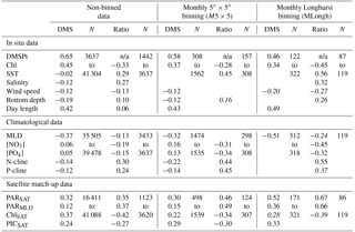
Table 1Correlation analysis (Pearson's r) for different data binning levels. Pearson's r with p value <0.01 are not shown; values in italic are ; n/a: not applicable. “Ratio” refers to log 10(DMS ∕ DMSPt). DMS, DMSPt, Chl, MLD, [NO3] and [PO4] were log 10 transformed; Pearson's r calculated on log 10-transformed variables were higher than those calculated on the same non-transformed variables, and similar in magnitude to Spearman's rank correlations. Bottom and nutricline depth values are shown as positive values (deeper is bigger). See the text for other acronyms.
Regression models were further optimized for global and regional domains using the bootstrap method followed by nonlinear optimization as described in Sect. S4. Selected models were then validated using an independent data subset composed of in situ DMS measurements and their satellite matchups (described in Sect. 3.1.3) and evaluated using a wide array of skill metrics (following Galí et al., 2015): R2, RMSE, mean absolute percentage error (MAPE), percentage bias and the slope of major axis (type II) linear regression between observations and model estimates (SlopeMA). All analyses were carried out using MATLAB R2013b.
2.3 Algorithm implementation
The newly developed DMSSAT algorithm (Fig. 2) was implemented to produce (i) a monthly global DMS climatology and (ii) several regional time series with 8-day resolution for the period 2003–2016. Further details and data sources can be found in Sect. S5 and Table S2.
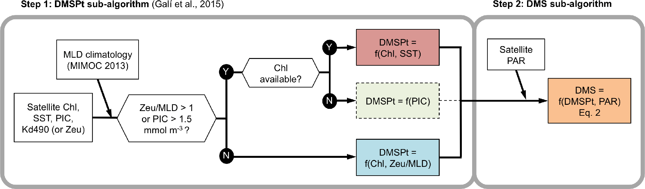
Figure 2Scheme of the DMSSAT algorithm. The algorithm proceeds in two steps: the DMSPt sub-algorithm (described by Galí et al., 2015 see Appendix A) and the DMS sub-algorithm (this study). Dashed lines mark the PIC-based equation of the DMSPt sub-algorithm, which in practice is not used when gap-free satellite Chl fields are used as input.
Global DMSSAT fields were computed using ocean color data from SeaWiFS (1997–2010 monthly climatology, 1∕12∘ grid), SST from AVHRR and the MIMOC monthly MLD climatology. We used SeaWiFS data to maximize the temporal overlap between the satellite-based DMSSAT climatology and the in situ data used to produce the L11 climatology, which span the period 1972–2010. Note, however, that DMSPtSAT climatologies derived from SeaWiFS and MODIS-Aqua are extremely similar (Galí et al., 2015). We established a reference DMSSAT run where ChlSAT was computed with a band-ratio algorithm (OC4-OCI standard NASA algorithm) and the euphotic layer depth (ZeuSAT) was computed as the 1 % penetration depth of 490 nm radiation (). The impact of this choice was evaluated with sensitivity tests where ChlSAT and ZeuSAT were calculated with the semi-analytical algorithms of Garver–Siegel–Maritorena (GSM; Maritorena et al., 2002) and Lee et al. (2007), respectively, which are more appropriate in optically complex waters. Observation gaps caused by low solar elevation at high latitudes in winter were left blank. Global monthly DMSSAT fields were averaged onto 1 and 5∘ grids for mapping and comparison to other DMS climatologies: the interpolated L11 climatology (Lana et al., 2011), and the climatologies derived with the empirical algorithms of Simó and Dachs (2002; SD02) and Vallina and Simó (2007b; VS07). The procedures used to calculate these datasets are briefly described in Sect. 3.2.
Regional DMSSAT time series between 2003 and 2016 were computed using daily MODIS-Aqua data (4.64 km) combined with the MIMOC MLD climatology. As done for the global implementation, we produced DMSSAT fields using both band-ratio and semi-analytical bio-optical products. We also performed a test comparing DMSPtSAT obtained with the MIMOC MLD climatology vs. model-derived MLD time series, showing little DMSPtSAT sensitivity (Fig. S1 in the Supplement). Since non-climatological satellite data contain gaps caused by cloudiness, we applied a binning and gap-filling procedure to obtain full coverage, such that the final regional time series had a resolution of 8 days and 27.8 km. We produced DMSSAT time series for the Bermuda Atlantic Time-series Study (BATS) station (31∘40′ N, 64∘10′ W) and for the Northern Hemisphere at latitudes >45∘ N. The latter dataset was then sampled at selected North Atlantic sites and at the Ocean Station P (OSP) in the NE Pacific (50∘ N, 145∘ W). Satellite time series were compared to the L11 climatology and to in situ DMS and DMSPt. These in situ data, kindly provided by the BATS (Levine et al., 2016) and OSP (https://www.waterproperties.ca/linep/, last access: 29 November 2017) teams, were not used in algorithm development.
3.1 Development and validation of the DMS sub-algorithm
3.1.1 Statistical exploration
We analyzed the correlation between potential predictor variables and log 10(DMS) or log 10(DMS∕DMSPt) (Table 1). This analysis systematically showed that (i) DMSPt was the best correlate of DMS (r=0.46 to 0.65), and (ii) surface PARSAT and mean PAR in the mixed layer (PARMLD) were the best correlates of the DMS ∕ DMSPt ratio (r=0.35 to 0.67). These correlation patterns remained across different binning levels, suggesting that DMS can be estimated, to first order, by the concentration of its phytoplanktonic precursor compound and by the PAR-dependent enhancement of DMSPt-to-DMS conversion. It is also noteworthy that the correlation between day length and the DMS ∕ DMSPt ratio was weak or non-significant. This supports the causal relationship between PAR and the DMS ∕ DMSPt ratio and discards other factors that might follow synchronous seasonal cycles.
Table 2Summary of fitted model coefficients and goodness-of-fit statistics. Different sets of coefficients were obtained by fitting the model log 10DMSPt+γPAR to observed DMS, DMSPt and PARSAT after applying different binning schemes. Equations (2f) and (2h) were derived using a different optimization procedure, applied to the global MLongh binned dataset and to the BATS station local dataset. The models implemented to calculate a global DMS climatology are denoted in italic, regional or local time series in bold.
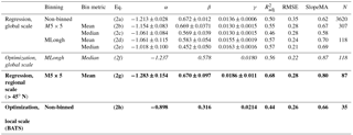
Guided by the correlation patterns, we established a base regression model expressed by the equation:
This model explained between 50 and 57 % of log 10(DMS) variance with an increasing level of data binning, and the corresponding RMSE ranged between 0.35 and 0.21 (Table 2).
We assessed whether the base model could be significantly improved by adding predictor variables and/or increasing model complexity. We started by adding a variable X to a linear model without interactions of the form . Variable X was chosen among those showing higher correlations to either DMS or the DMS ∕ DMSPt ratio: SST, nitrate concentration, nitracline depth, salinity, wind speed and PICSAT (Table 1). Although this analysis led us to discard additional predictor variables, its results are briefly described below and compiled in Table S4 for the sake of completeness. With non-binned data, all the additional variables entered regression models with significant coefficients, but only salinity, wind speed and PICSAT produced significant decreases in RMSE and AIC. With MLongh binned data, only SST and PICSAT entered with significant coefficients. Yet none of the additional variables improved simultaneously the R2 adj, RMSE and AIC skill metrics with respect to the base model. Increasing model complexity through addition of interaction and quadratic terms, or by adding a fourth variable, generally resulted in minor improvements or erratic changes in model performance (results not shown). Invariably, DMSPt and PAR were the only variables with highly significant coefficients () regardless of the binning scheme or the inclusion of additional variables.
As a corollary, the use of PARMLD instead of PARSAT slightly degraded model skill (Table S4). Although PARMLD is a priori a more realistic metric of light exposure, it is possible that the use of climatological MLD degraded the PARMLD estimates. Another potential explanation is the episodic nature of oceanic vertical mixing, which requires the distinction between the actively mixing layer, which is defined by higher turbulence than in the ocean interior, and the mixed layer, here termed MLD and defined by the vertical homogeneity of regular temperature–salinity profiles (Brainerd and Gregg, 1995; Sutherland et al., 2014). This distinction implies that, on occasion, mean light exposure at the sea surface is better approximated by surface PARSAT than by PARMLD. After these considerations we excluded PARMLD from our algorithm, and focused on optimizing Eq. (2).
Finally, note that PARSAT is used in our algorithm both as a direct driver of DMS cycling processes and as a proxy for UVR-driven processes (e.g., Archer et al., 2010; Galí et al., 2013; Royer et al., 2016). For obvious astronomical reasons, incident PAR and UVR are strongly correlated. Attenuation of PAR and UVR in the atmosphere, first, and in seawater, afterwards, also covary (Kirk, 2011), so that plankton UVR exposure is to first order well correlated to PAR.
3.1.2 Implications of the model structure
Here we analyze the physical and biogeochemical meaning of Eq. (2) coefficients in view of their optimization for diagnostic purposes (3.1.3).
-
The intercept (α) acts to adjust the magnitude of DMS concentrations by a fixed proportion everywhere; e.g., increasing α by log 10(1.10) would raise estimated DMS concentrations by 10 % globally.
-
The log 10DMSPt coefficient (β) expresses the nonlinear relationship between DMS and DMSPt. Fitted β is smaller than 1 regardless of the binning applied. For a constant PAR, this implies that DMS increases more slowly than DMSPt (Fig. 3a) and that the DMS ∕ DMSPt ratio decreases nonlinearly and approaches an horizontal asymptote as DMSPt increases (Fig. 3a). This behavior implicitly represents the change in DMSPt-to-DMS conversion efficiency depending on the biomass and structure of the microbial plankton community.
-
The PAR coefficient (γ) expresses the DMSPt-independent modulation of DMS concentration. Fitted γ is larger than 0, meaning that the PAR sensitivity increases exponentially with PAR, regardless of DMSPt (Fig. 3b). Incident PAR is positively correlated to shallow mixing at the global scale, and to seawater transparency at low latitudes (but not at high latitudes). Thus, nonlinear PAR sensitivity possibly embodies the enhancement of sunlight exposure by shallow mixing and deeper PAR (and UVR) penetration. In summary, γ represents stress-driven DMS production.
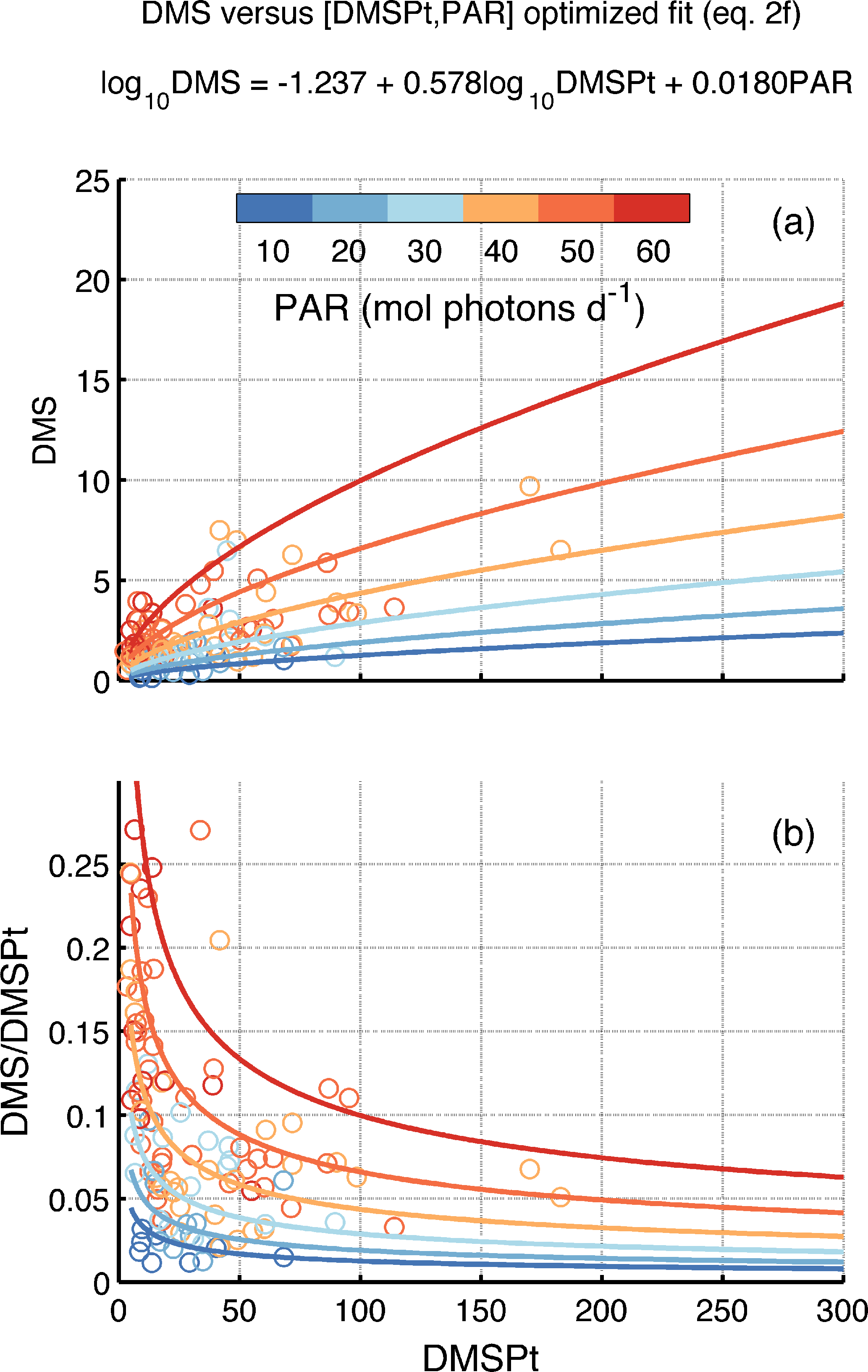
Figure 3Relationship between DMS, DMSPt and PAR as represented in the DMSSAT algorithm. (a) DMS vs. DMSPt and (b) DMS ∕ DMSPt ratio vs. DMSPt, as a function of PAR. Colored circles represent the medians of in situ data binned by Longhurst province and month, and lines correspond to the model predictions. PAR levels are indicated in the color bar.
In biogeochemical terms, Eq. (2) implies maximal DMS ∕ DMSPt ratios when/where low DMSPt and high PAR co-occur. In biogeographic terms (Fig. 1), highest DMS ∕ DMSPt ratios are found in oligotrophic areas of the Trades biome, where low DMSPt concentrations prevail (<20 nM). Low DMSPt concentrations are also found in winter at high latitudes in deeply mixed waters, but the corresponding low irradiance results in DMS ∕ DMSPt < 0.05. At the high DMSPt concentrations that occur at high latitudes in summer (>100 nM), the DMS ∕ DMSPt ratio is generally <0.1.
As shown in Table 2, Eq. (2) coefficients change systematically as the binning spatial scale increases. To further explore the interrelationship between the model coefficients, we used the bootstrap method to produce 105 sets of regression coefficients for the MLongh dataset. The scatter plots between α, β and γ resulting from the 105 bootstrapped regressions confirmed that covariation between the coefficients is non-random, such that fitted β and γ are negatively correlated to α (Fig. S2). These trade-offs should be kept in mind when optimizing our model for global or regional implementation.
3.1.3 Optimization and validation
By definition, least squares regression minimizes the RMSE, but it has been shown that regression models derived in this way do not necessarily have the best skill (Jolliff et al., 2009). Therefore, we devised an alternative nonlinear optimization procedure (Sect. S4). To obtain realistic solutions, we constrained the optimized coefficients to the confidence intervals derived from the bootstrapped regressions for the MLongh dataset (Fig. S2). The resulting optimal model (Eq. 2f) had higher DMSPt (β) and PAR (γ) coefficients and a smaller intercept (α), and moved the modeled DMS concentration closer to the 1:1 agreement line without degrading either RMSE or R2 (Table 2).
We validated the different versions of Eq. (2) (Table 2) by comparing DMSSAT against in situ DMS using an independent subset of the database. Since the complete DMS algorithm proceeds in two steps (Fig. 2), its validation must take into account uncertainty in variables used as input to the DMSPtSAT sub-algorithm. Galí et al. (2015) showed that, apart from the inherent algorithm uncertainty, most uncertainty in DMSPtSAT (RMSE ≤0.3 in log 10 space) results from error in ChlSAT. Thus, the validation subset was defined according to three criteria: (i) satellite matchup data used as input to the algorithm (ChlSAT, Kd,490, PARSAT and SSTSAT) were available; (ii) in situ DMSPt was not available – thus excluding the data used for model fitting; (iii) in situ DMS and Chl were available. We used in situ Chl concentration to constrain the uncertainty in ChlSAT used as input to the algorithm. Indeed, this procedure progressively reduced the size of the validation subset as the maximum ChlSAT error tolerated decreased. Uncertainty arising from PARSAT could not be assessed because the current database lacks in situ PAR measurements. Frouin et al. (2003) reported an error of ±15 % (<10 % for weekly and monthly periods), with negligible bias for PARSAT, suggesting it is a minor source of uncertainty.
Figure 4a summarizes the validation results for the best-performing regression model (Eq. 2e) and its optimized version (Eq. 2f). Supporting our assumption, DMSSAT skill metrics improved as the maximum tolerated ChlSAT RMSE decreased from 0.5 to 0.2 (Fig. 4). With ChlSAT RMSE smaller than 0.2, the statistics showed erratic behavior owing to reduced sample size. Other skill metrics (not shown in Fig. 4) showed comparable trends.
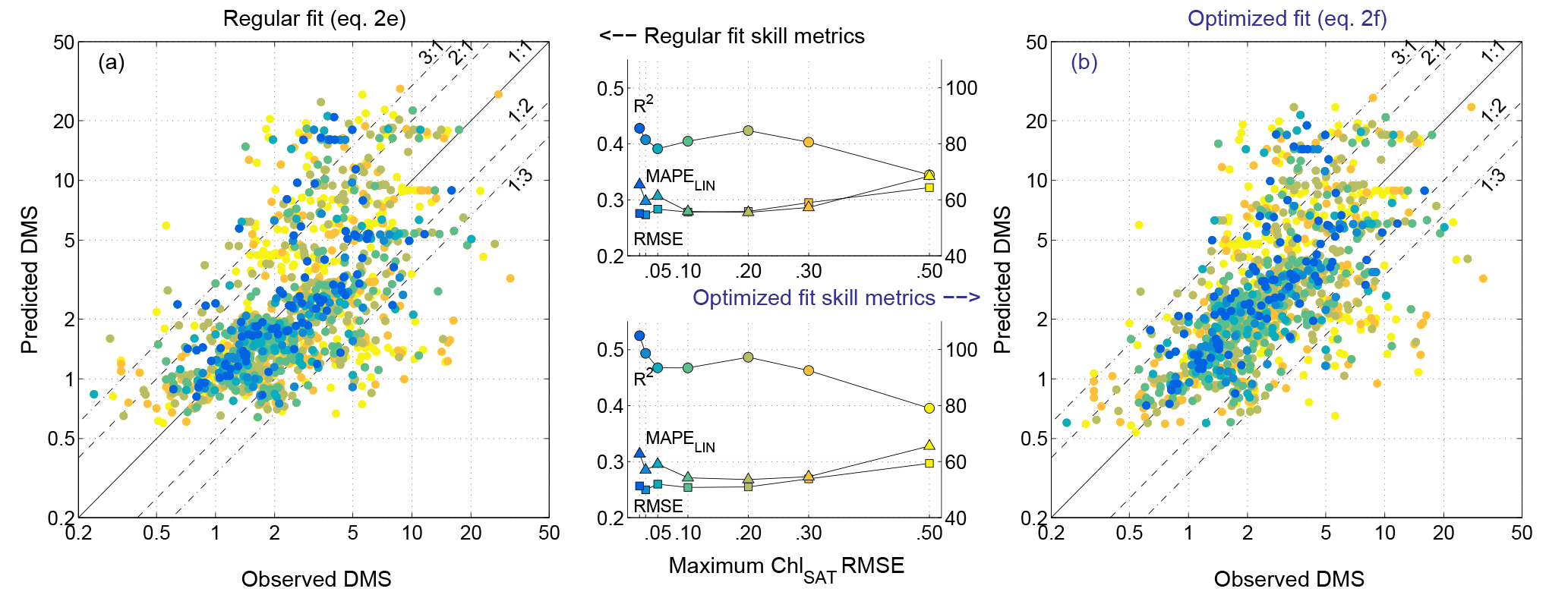
Figure 4Algorithm validation results constrained by the uncertainty in satellite-retrieved Chl. (a) Equation (2e), derived from regular multiple regression; (b) Eq. (2f), obtained through an optimization procedure. The scatter plots compare non-binned data and model estimates, color-coded depending on the maximum tolerated error in ChlSAT with respect to Chl in situ, as shown in the x axis of the center plots. The center plots show the performance of the DMS algorithm for increasing error in ChlSAT, evaluated with different skill metrics: the log 10 space R2 and RMSE (left y axis) and the linear space MAPE (right y axis). N increases from 86 to 1293 as the tolerated ChlSAT error increases.
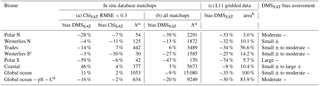
Table 3Relative deviation (“bias”) of the global-scale optimized DMSSAT algorithm across ocean biomes when evaluated against the in situ database (a and b) and against the L11 monthly climatology (c). Comparison with the in situ database was done using either (a) satellite matchups with ChlSAT error constrained with respect to in situ Chl or (b) all ChlSAT matchups, regardless of the availability of in situ Chl. The last column shows a qualitative overall assessment of DMSSAT bias, based on columns (a–c), classifying the most likely magnitude and sign as small ± (±10 %), moderate (10 to 40 %, either + or −) or large (>40 %, either + or −).
a For the database comparisons,
the amount of data (N) available for validation in a given region depends
on the total amount of measurements, the proportion of data points with
satellite matchups and, for the constrained case, the fraction of matchups
where ChlSAT has log 10RMSE<0.3 compared to
concurrent Chl in situ. Samples with available DMSPt measurements were
excluded because they were used in model fitting and
optimization.
b For the global climatology comparison we report the percentage of
ocean area, excluding pixels that could not be observed by
satellites (high-latitude winter).
c Samples where DMSPt was measured (not excluded) for this
biome due to the small amount of data. Removing them would leave N=13.
d Global ocean minus Polar S and Coastal
biomes.
The optimized model coefficients (Eq. 2f) increased R2 and reduced RMSE with respect to the regression-derived coefficients, achieving a maximal R2 of 0.53 and a minimal RMSE of 0.25 for error-free ChlSAT (log 10-space non-binned data; Table S5). Corresponding best scores in linear space were R2=0.24 and RMSE =3.4 nM. These linear space statistics might be interpreted as a sign of poor performance, but it should be noted that they were strongly affected by a small fraction of highly biased estimates. Removing the most biased estimates (8 % of points beyond a factor of 3 from real measurements; Fig. 4) increased the linear space R2 to 0.42–0.53 and decreased the RMSE to 1.8–2.3 nM across the full range of ChlSAT error, with MAPE of 34–41 % and relative bias of −1 to 7 %. Altogether, these statistics illustrate the good performance of the DMSSAT algorithm and the greater robustness of log-space statistics. The global-scale optimized algorithm had a mean-normalized standard deviation of 1.06–1.14 (log 10 space), meaning that the spread of DMSSAT nearly matched that of in situ DMS concentrations.
Table 4Mean area-weighted DMS concentrations for different climatological datasets and domains. Different results for the DMSSAT algorithm were obtained using alternative approaches for retrieving chlorophyll a concentration (ChlSAT) and the euphotic layer depth (ZeuSAT). Results (based on gridded data) are shown for the global domain, the Longhurst Coastal biome and, within it, areas shallower than 200 m (shelves); n/a: not applicable.
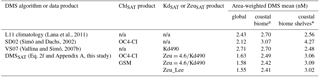
* The Longhurst Coastal biome represents about 10.4 % of the global ocean area, of which one third is shallower than 200 m (3.5 % of global area).
Table 3 summarizes a detailed analysis of algorithm bias in different biomes. When ChlSAT error was constrained to RMSE <0.3, DMSSAT showed a global mean bias of 11 % (with a global mean bias of 2 % in ChlSAT itself). DMSSAT bias was negligible in the Westerlies biomes and larger than ±10 % in the other biomes, where its sign often matched that of ChlSAT bias. When DMSSAT bias was assessed using all available matchups, irrespective of ChlSAT error, we obtained a global bias of −9 %. In some biomes, the sign and magnitude of DMSSAT bias changed when ChlSAT error was not constrained, indicating the influence of input satellite data. Assuming that ChlSAT matchups (N∼15 000) are a random sample of the database between 1997 and 2012 (N∼24 000), this analysis suggests that global DMSSAT bias likely ranges between −9 and 11 %.
3.2 Global climatologies
We implemented the global-scale optimized algorithm (Eq. 2f) using the SeaWiFS climatology. As shown in Fig. 5 and 6, DMS concentrations around ∼2.5 nM prevail during the astronomical spring and summer in each hemisphere, decreasing to around 1 nM in fall and <1 nM in winter. The seasonal cycle has wider amplitude at high latitudes and is nearly flat in the tropical oceans (see also Fig. S3). Regional enhancement of DMS concentrations occurs in some coastal and shelf areas, equatorial and eastern boundary upwellings, close to the subtropical front in austral summer (40∘ S) and in the subpolar North Atlantic in boreal summer (60∘ N). The global mean area-weighted DMSSAT concentration is 1.63 nM (median and geometric mean of 1.36 nM). This global mean decreases by less than 5 % when semi-analytical ChlSAT and ZeuSAT products are used instead of our reference products, but larger deviations occur in the Coastal biome, particularly in shallow areas, associated with optically complex waters (Table 4).
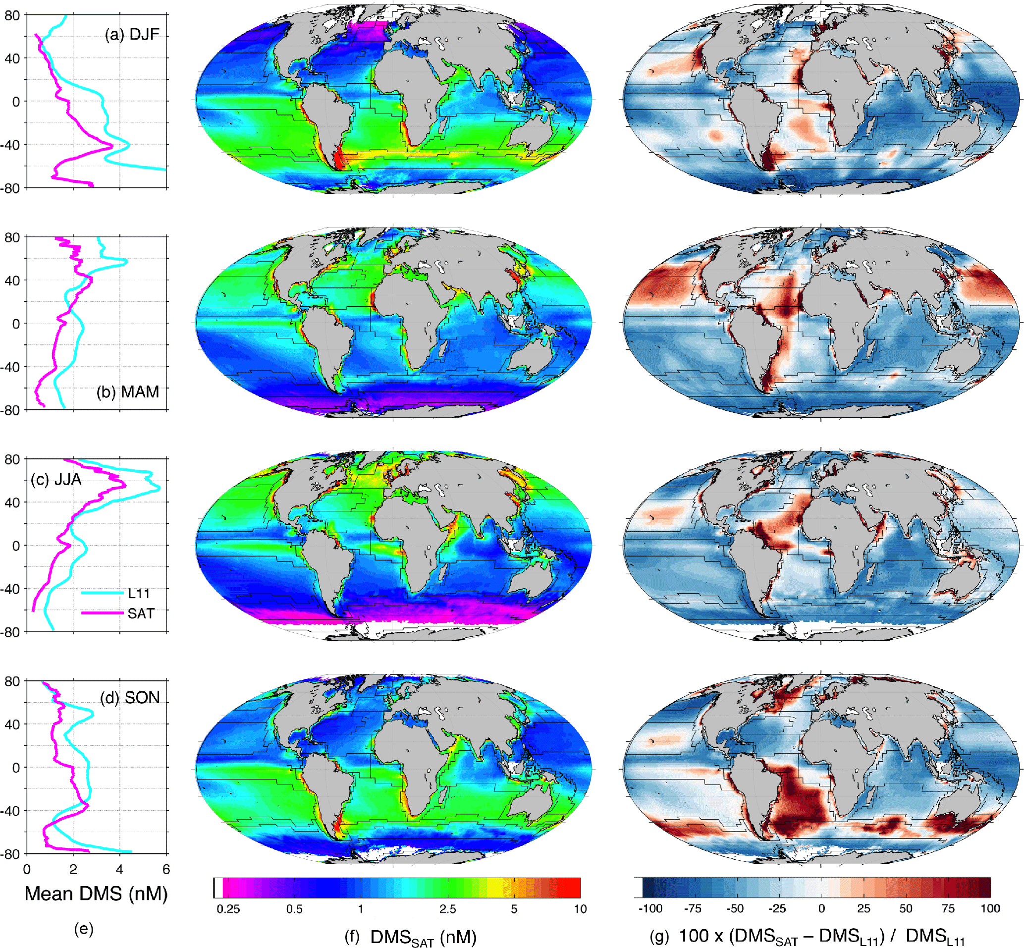
Figure 5Global DMSSAT concentration fields by season. (a) December–February (DJF); (b) March–May (MAM); (c) June–August (JJA); (d) September–November (SON). Each row contains mean latitudinal profiles for the L11 climatology and DMSSAT (left); DMSSAT concentration maps (center); and maps of the percentage difference between DMSSAT and the L11 climatology (right).
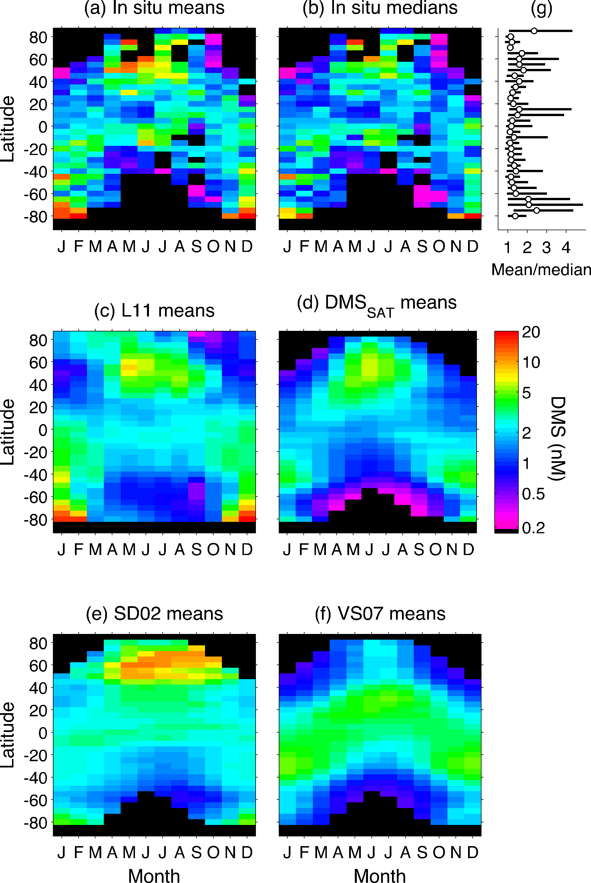
Figure 6Hovmöller diagrams comparing climatological DMS fields (monthly 5∘ latitude bins). (a) In situ database means, (b) in situ database medians, (c) L11 climatology, (d) DMSSAT algorithm, (e) SD02 algorithm and (f) VS07 algorithm. Panels (a–f) share the same color scale; the black background indicates no data. Panel (g) shows the average and range of monthly mean∕median ratios (shown in panels a and b) in each latitude band. Geometric means of in situ binned data (b) are similar to bin medians.
3.2.1 Comparison to the L11 climatology
The L11 DMS climatology (Lana et al., 2011) was calculated using an objective interpolation procedure similar to that used in prior climatologies (Kettle et al., 1999; Kettle and Andreae, 2000). An initial template, called first-guess field, was obtained by calculating the monthly mean DMS in each Longhurst province. The gaps were filled through temporal interpolation and, in provinces with too few documented months, the seasonal cycle was extrapolated by scaling that of neighboring provinces. Objective interpolation was then applied by searching measurements within a 555 km radius, weighting them inversely to the distance from a given grid point, and the resulting global fields were repeatedly smoothed.
The global mean area-weighted DMSL11 concentration is 2.43 nM (median 1.88 nM, geometric mean 1.83 nM). Thus, mean DMSSAT concentration is globally 33 % lower than DMSL11 (Tables 3 and 4). The largest and smallest differences occur in the southern polar and the Coastal biomes, respectively (Table 3).
The disagreement between the DMSL11 and DMSSAT climatologies varies depending on the regions and on the spatial–temporal scales compared. Despite the general offset, the seasonal latitudinal profiles (zonal means) of DMSL11 and DMSSAT have similar shapes, and agree very well in June through August. Comparison by means of Hovmöller diagrams (Fig. 6) shows a remarkable qualitative agreement in their month-by–latitude patterns, except for the polar austral summer. Figure 6 also reveals smaller disagreements in the Arctic Ocean in winter–spring and in the equatorial band during most of the year, with lower concentrations in DMSSAT in both cases. The most striking regional disagreements appear when DMSSAT and DMSL11 are compared by means of seasonal anomaly maps (Fig. 5). The sign of the DMSSAT−DMSL11 divergence changes from positive to negative in a patchy pattern, often following the boundaries of the Longhurst biogeochemical provinces.
3.2.2 Comparison to the SD02 climatology
The SD02 algorithm (Simó and Dachs, 2002) was designed to estimate DMS from MLD and ChlSAT using two different equations depending on the Chl∕MLD ratio,
such that DMS increases linearly with the Chl∕MLD ratio in stratified productive conditions (e.g., high latitudes in summer) and inversely with MLD in typical oligotrophic conditions.
Validation of SD02 with the same dataset used for DMSSAT indicates that it explains less variance (log 10 R2 of 0.22–0.31) but has similar RMSE and MAPE (Table S5). Globally, DMSSD02 is characterized by a bimodal distribution (Fig. 7), with an area-weighted mean of 2.12 nM, 13 % lower than DMSL11 (Table 4). SD02 estimates are in good agreement with the L11 climatology at tropical and temperate latitudes. In the southern Westerlies biome, however, prevailing deep vertical mixing and low Chl cause SD02 to underestimate DMS throughout the productive season (Figs. 6 and S3). Another feature of SD02 is the high DMS concentration in northern polar latitudes through late summer and fall, caused mainly by the shallow MLD due to freshwater-driven stratification. As DMSSAT, DMSSD02 suffers from negative bias in the Antarctic biome during the productive season (November through February).
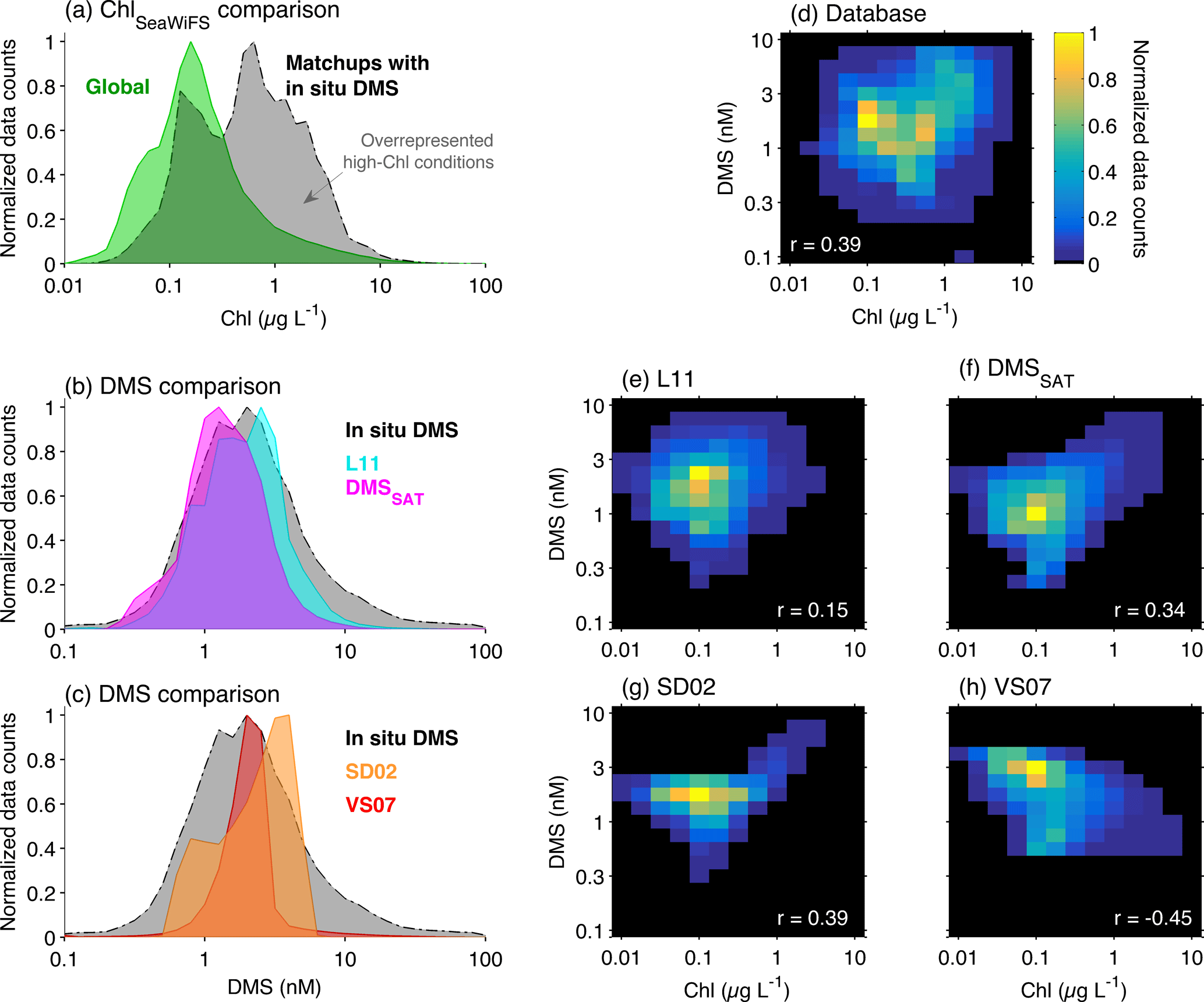
Figure 7Histograms illustrating the relationship between DMS and Chl in the global ocean. (a) Global SeaWiFS 1997–2010 ChlSAT climatology and SeaWiFS ChlSAT matchups for the in situ DMS database; (b) Global L11 and DMSSAT climatologies and in situ DMS database; (c) Global SD02 and VS07 climatologies and in situ DMS database; (d) bivariate histogram of in situ DMS vs. corresponding SeaWiFS ChlSAT matchups; (e–h) bivariate histograms of the global SeaWiFS ChlSAT climatology vs. climatological DMS from (e) L11, (d) DMSSAT, (e) SD02 and (f) VS07 algorithms. In (d–h), the correlation coefficient (Pearson's r) between DMS and Chl in each dataset is super-imprinted in white.
3.2.3 Comparison to the VS07 climatology
Vallina and Simó (2007b) reported a globally valid linear relationship between DMS concentration and the solar radiation dose (SRD) in the upper mixed layer in the global ocean, according to the equation:
This numerical relationship was not meant to be used as an empirical algorithm but as evidence for the emerging response of ecosystem DMS production to changes in solar radiation. However, the fact that SRD explained a large part of the variance of DMS concentration across regions and seasons prompted its use in global warming projections (Vallina et al., 2007). SRD is analogous to PARMLD (Eq. 1), but replacing PARSAT by total shortwave irradiance (EdSW; W m−2). Here we implemented VS07 with two variations: (i) we used Kd490SAT instead of a fixed Kd (note that in phytoplankton-rich and continentally influenced waters, Kd490SAT is generally higher than the fixed Kd =0.06 m−1 used by Vallina and Simó, 2007b); (ii) we estimated EdSW from PARSAT by converting the latter to units of W m−2 (Morel and Smith, 1974) and then applying a constant EdSW ∕ PARSAT ratio of 1∕0.43 (Kirk, 2011).
VS07 shows poorer performance than DMSSAT and SD02 when validated with individual measurements (Table S5). It produces rather uniform DMS fields compared to the other climatologies (Figs. 6 and 7c), with mean area-weighted concentration of 2.71 nM (Table 4). VS07 performs well in the Westerlies biome, especially in the Northern Hemisphere, but invariably overestimates (underestimates) DMS in the Trades (Polar) biomes (Fig. S3).
3.3 Regional DMSSAT time series
We selected different regions to test the DMSSAT algorithm based on the following criteria: the abundance of in situ data (subpolar North Atlantic), the existence of seasonal and multiannual time series (Ocean Station P and BATS station), and the challenges posed by intra- and interannual variability of phytoplankton and DMS(P) in each region.
3.3.1 Subpolar Atlantic and Pacific
We used MODIS-Aqua data to produce a 14-year DMSSAT time series (and the corresponding climatology) for the Northern Hemisphere at latitudes >45∘ N. In this regional implementation we used a different set of coefficients, obtained from regression of M5×5 binned data restricted to latitudes >45∘ N (Eq. 2g, Table 2). These regional coefficients largely corrected the negative bias observed with globally optimized coefficients. In this case, further optimization did not lead to significant improvement. We then sampled the resulting time series in some representative regions: three rectangles with an area of ∼200 000 km2 each, located along the 50–56∘ N band in the North Atlantic, and the Ocean Station P (OSP, 50∘ N, 145∘ W) in the NE Pacific.
Figure 8 shows the seasonal cycles of DMSSAT, DMSPtSAT and ChlSAT in selected North Atlantic areas: (a) the deep waters of the northwest Atlantic drift, (b) the shelf break west of Ireland, and (c) the shallow southern North Sea. We observe good agreement between the 14-year DMSSAT climatology and the L11 climatology, except in the southern North Sea where DMSSAT is too high through summer and fall. DMSSAT reproduces well the east–west variation in the temporal lag between the annual peaks of DMS and Chl, with a lag of up to 4 months in the southern North Sea. The most salient result is however the wide interannual variability of the DMSSAT seasonal cycles. Estimated DMSSAT concentrations during the productive season vary by up to 3-fold between years (see variability metrics in Fig. 8), and the annual DMSSAT peak can occur within a temporal window of 2–3 months. Although years with a major peak in spring–summer are the norm, a second peak in late summer is not unusual. Additional validation supports the good performance of DMSSAT in the subpolar North Atlantic (Fig. S4), lending credit to satellite-determined variability patterns.
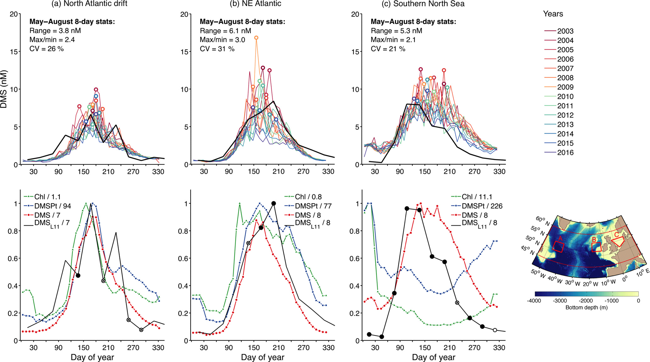
Figure 8Interannual DMSSAT variability in the subpolar North Atlantic. (a) Northwest Atlantic drift, (b) shelf break west of Ireland, (c) southern North Sea shelf. Top panels show individual years between 2003 and 2016 determined from 8-day MODIS-Aqua data, differentiated by color, and the mean seasonal cycle according to the L11 DMS climatology (black); colored circles mark the peak of each seasonal cycle. Bottom panels show the mean annual cycles of ChlSAT, DMSPtSAT, DMSSAT and the L11 DMS climatology. Each variable is divided by its maximum, shown by the number in the quotient; a common scaling factor is used for DMSSAT and DMSL11. Markers on the L11 line indicate the amount of in situ data on which the L11 climatology is based in a given month: no data, i.e., month filled through interpolation (no marker); 1–9 measurements in a single year (empty circles); ≥10 measurements in a single year (crossed circles); and ≥10 measurements distributed in different years (filled black circles). Red polygons on the map show the 3 selected areas and the larger region used for the validation scatter plots (see Fig. S4).
We used the same MODIS-Aqua dataset to analyze the mean seasonal cycle and the interannual variability at OSP (Fig. 9a–c), where DMS has been measured around February, June and August since 1996. DMSSAT captures in situ DMS concentrations in February and June but suffers from low bias in August. Examination of August measurements during the 2005–2016 period suggests the existence of two regimes: 8 years with in situ DMS of 6.6±1.1 nM, about twice as high as DMSSAT, and 4 years with in situ DMS of 16.1±4.8 nM, about 6-fold higher than DMSSAT. Local tuning of Eq. (2) using OSP data could not increase DMSSAT in August–September without degrading its performance in other months.
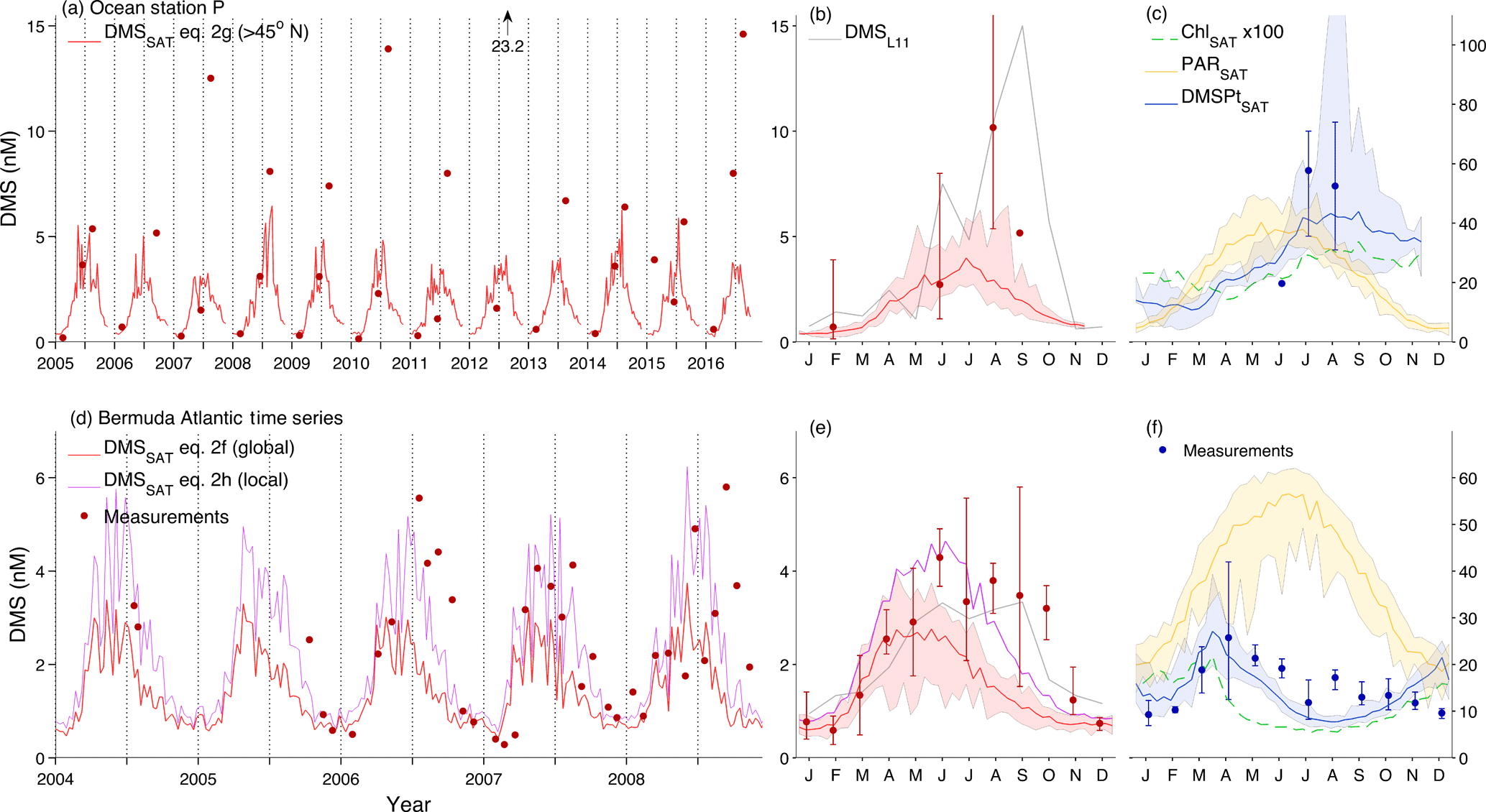
Figure 9DMSSAT vs. in situ data at long-term research stations. (a–c) Ocean Station P in the northeast Pacific (50∘ N, 145∘ W); (d–f) BATS station (31∘40′ N, 64∘10′ W). (a, d) compare DMSSAT estimates to in situ measurements; (b, e) compare monthly DMS means (i.e., climatologies) derived from DMSSAT (2003–2016 MODIS-Aqua data), in situ data (available measurements between 2003–2016) and the L11 climatology; (c, f) show the corresponding ChlSAT, DMSPtSAT and PARSAT climatologies (2003–2016) and in situ DMSPt. Lines and shaded envelopes show the mean ± range of satellite-derived data; filled circles and error bars show the mean ± range of available in situ data. DMS and DMSPt are in nM units, Chl in µg L−1 and PAR in mol photons . In addition to public OSP data (three DMS measurements per year generally available between 2005 and 2016) we show DMSPt data reported in published studies (Asher et al., 2017; Levasseur et al., 2006; Royer et al., 2010). BATS data are comprised of the monthly 2005–2008 time series (Levine et al., 2016) and cruise data from the vicinity of BATS station in July 2004 (Bailey et al., 2008; Gabric et al., 2008).
Finally, note that these time series were calculated using semi-analytical bio-optical products (see section S5). Using the band-ratio Chl algorithm for MODIS (OC3) gave very similar results in deep ocean regions but 70 % higher concentrations in the shallow southern North Sea, possibly due to interference of non-algal materials on OC3 Chl retrieval (data not shown).
3.3.2 Bermuda Atlantic Time-series Study
Using the globally tuned coefficients (Eq. 2f), DMSSAT reproduces the shape of the mean seasonal cycle at the oligotrophic BATS station but underestimates DMS by around 2-fold between June and October (Fig. 9d and e). In August, part of this bias can be attributed to DMSPtSAT (Fig. 9f). However, replacing DMSPtSAT by in situ DMSPt raises DMSSAT by only 17 %, indicating that most of the underestimation is caused by the DMS sub-algorithm. Optimizing the coefficients using local data (Eq. 2h; Sect. S4) improves the model–data fit by decreasing the DMSPt coefficient and increasing the PAR coefficient. Indeed, different studies have shown that irradiance suffices to explain most of the DMS seasonal cycle at BATS (Galí and Simó, 2015; Toole and Siegel, 2004; Vallina and Simó, 2007b). Regarding interannual variation, it is of note that the locally tuned DMSSAT is in excellent agreement with in situ data throughout 2007 and in June through August in all years, while the underestimation persists in September and October of 2006 and 2008.
The DMSSAT algorithm captures in situ variability (Figs. 4–9 and S3) using a small set of predictor variables (Fig. 2). Moreover, it reproduces the mismatch between DMS and Chl such that, at a given ChlSAT concentration, determined DMS can vary by up to 40-fold. This mismatch is larger than that produced by the SD02 or the VS07 algorithms, but still smaller than in the database (Fig. 7d–h). The progressive dissociation between ChlSAT and DMS imposed by the two-step algorithm, and the nonlinear relationships embodied in Eq. (2) (Fig. 3), allow DMSSAT to produce a DMS peak in the right concentration range in summer across different latitudes, despite order-of-magnitude variations in chlorophyll concentration (Le Clainche et al., 2010).
Independent validation using satellite matchups suggests that DMSSAT estimates are globally within ±10 % of in situ measurements. However, this is at odds with the global mean bias of −33 % suggested by comparison to the L11 gridded climatology. In some regions, assessments of DMSSAT bias based on comparison to matchups and to L11 are consistent (Table 3), indicating shortcomings of the algorithm and/or in input satellite data. For instance, the globally optimized coefficients produce too low DMS in northern high latitudes, which we solved through regional tuning, building on the relative abundance of DMS(P) measurements north of 45∘ N (Table 2, Fig. 8). In southern high latitudes, too-low DMSSAT primarily results from the negative ChlSAT bias (estimated at 50 % by Johnson et al. (2013) and −56 % in our matchup dataset). Improving DMSSAT in this region would require, in the first place, the improvement of bio-optical algorithms and an important sampling effort to better document DMS(P) dynamics (Fig. 1; Jarníková and Tortell, 2016). In contrast to high latitudes, database matchups in the Westerlies and Trades biomes suggest smaller DMSSAT bias than comparison to L11 gridded data (Table 3). While some of this bias certainly arises from too-low DMSSAT in late summer at specific locations (Fig. 9), it is also plausible that divergences between DMSSAT and DMSL11 arise from regional biases in the interpolated climatology.
In what follows we pinpoint the strengths and weaknesses of our novel approach focusing on two aspects. In Sect. 4.1 we examine how geo-statistical shortcomings of the in situ DMS database cause bias in the L11 interpolated climatology, highlighting the advantages of DMSSAT and paving the way towards improving gridded DMS fields. In Sect. 4.2 we speculate about potential causes behind high DMS ∕ DMSPt ratios in late summer and early fall. This exercise shows our limited capacity to account for relevant biogeochemical processes and explain their interannual variation using satellite data, and identifies knowledge gaps that need to be tackled to improve diagnostic and prognostic modeling of oceanic DMS(P). The rationale is that both kinds of issues (“geo-statistical” and “biogeochemical”) are highlighted by discrepancies among in situ data, L11, and the macroecological relationships embodied in our algorithm.
4.1 Known sources of error and bias: interpolated climatology vs. DMSSAT
Global DMS fields estimated by the L11 climatology and by the DMSSAT algorithm show remarkable geographic differences (Fig. 5), and their mean concentrations differ by a factor of ∼1.5. Particularly, changes in the sign of the DMSSAT–DMSL11 anomaly often follow the somewhat artificial boundaries of the Longhurst biogeochemical provinces. As explained below, regional and global biases in L11 arise from the application of objective interpolation procedures to a global dataset characterized by (1) the right-skewed distribution of DMS concentrations (Kettle et al., 1999; Fig. 7), (2) the small amount of monthly data available in many biogeochemical provinces (Fig. 1), (3) the absence of repeat measurements in most oceanic regions (Halloran et al., 2010), (4) the low spatial resolution of most DMS datasets and (5) the preferential sampling of DMS-productive conditions.
A primary drawback for the calculation of interpolated climatologies is the overrepresentation of biologically productive conditions in the sea-surface DMS database. This sampling bias is clearly illustrated by comparing SeaWiFS-retrieved Chl concentration in the global ocean and in the database matchups (Fig. 7a). If we assume that SeaWiFS matchups (N=11 600) represent a random sample of the DMS database (N=41 304), and considering the global positive correlation between Chl and DMS (Fig. 7d), this implies a sampling bias towards high DMS concentrations. The bias is largest when the comparison is restricted to the spring–summer semester of each hemisphere, when the median ChlSAT is 0.19 in the global SeaWiFS climatology and 0.74 in the DMS database matchups. This is the period when DMS peaks and has more influence on mean annual DMS concentration.
Sampling bias is intertwined with the right-skewed distribution of sea-surface DMS concentrations (Fig. 7b) and the poor spatial resolution of most in situ DMS datasets. Spatial averaging, justified by data scarcity, is appropriate when applied over small or sufficiently homogeneous regions. However, when applied over a large and potentially heterogeneous Longhurst province, it can propagate the sampling bias over the entire province and up to the global scale. As illustrated in Fig. 6g, the mean DMS concentration in M5×5 bins is systematically higher, by 40 % on average, than the corresponding median. Province-level averaging converts the long tail of high in situ DMS concentrations into too-large province means, such that the global mode of DMSL11 is similar or even higher than that of in situ DMS (Fig. 7b).
The influence of extreme in situ DMS concentrations is maximal in productive regions, where mean∕median ratios of around 4 are observed in M5×5 bins (Fig. 6g). In these regions, sharp productivity gradients and dynamic ecosystem processes complicate the task of sampling DMS through all appropriate scales (Nemcek et al., 2008), suggesting the need to apply finer-scale or dynamic regionalization (Devred et al., 2007) prior to interpolation. Emerging biogeochemical relationships, like that between net community production and DMS observed by Kameyama et al. (2013) in the northeast Pacific, might assist DMS interpolation and determination, but require validation across contrasting regions and relevant scales (Asher et al., 2017). In low-latitude oligotrophic areas where DMS shows reduced spatial variability (Royer et al., 2015), the method used to construct interpolation-based climatologies (Kettle et al., 1999; Lana et al., 2011) seems appropriate regarding spatial resolution.
In the temporal domain, the calculation of interpolated climatologies is complicated by two factors: poor interannual coverage, i.e., the scarcity of DMS measurements repeated in different years in a given region; and poor seasonal coverage, i.e., the scarcity of fully resolved seasonal cycles. Seasonal coverage is limited at the province level (see Table 1 in Lana et al., 2011) and obviously worse in 5∘ bins (Fig. 1d). Regarding interannual coverage at the MLongh level, 42 % of the province–month bins contain measurements from a single year, 21 % from two years and 37 % from three or more years. Thus, data from one or two years are often assumed representative of the mean ecosystem state in interpolated climatologies, which is probably not the case in regions with wide interannual variability or long-term trends (Vantrepotte and Mélin, 2011). While this does not necessarily bias global DMS fields, it can produce artificial seasonal cycles. For example, L11 suggests the existence of early spring and fall DMS peaks in the North Atlantic drift area, which result from interpolation from neighboring regions (Fig. 8a). In contrast, DMSSAT suggests these are improbable (spring) or infrequent (fall) features. Another example is found at OSP, where DMSL11, based on measurements made before 2003, is in poor agreement with measurements made between 2005 and 2016. In February and June, DMSSAT is in better accordance with in situ DMS data at OSP (Fig. 9a and b).
In summary, caution has to be taken when comparing DMS measurements, their derived climatological products, and independent model estimates that are not collocated in time. This temporal mismatch may partly explain the poor correlation between modeled DMS climatologies, on one hand, and the DMS database and DMSL11 climatology, on the other (Tesdal et al., 2016). Note that the latter study compared DMS fields binned into monthly boxes (M5×5), such that 82 % of the bins contained measurements from a single year.
Compared to interpolated climatologies, DMSSAT provides a robust means to estimate DMS concentrations in sparsely sampled areas because it relies on satellite observations and macroecological relationships. The resulting DMS fields are in better accordance with natural gradients in plankton abundance (biogeography, phenology) and environmental forcing, as long as the models can account for the driving factors, as discussed below.
4.2 Unknown sources of error: how far can we go with remote sensing algorithms?
By testing DMSSAT in challenging biogeochemical settings (Fig. 9), we identified its main drawback: the failure to reproduce high DMS, and more specifically DMS ∕ DMSPt ratios higher than 0.3, at intermediate PAR levels (Fig. 3), as observed between midsummer and early fall at BATS and OSP in some years. This limitation can hardly be fixed without identifying the underlying biogeochemical processes, which are not necessarily the same in these contrasting biogeochemical regimes. Although this feature is probably not widespread (see Fig. 2 in Lana et al., 2011), its occurrence in emblematic time series stations warrants further discussion.
A common explanation could be the underestimation of irradiance effects, caused by the use of sea-surface PARSAT rather than PARMLD as DMS predictor variable. For instance, a delay of seasonal mixing, associated with deeper irradiance penetration, could enhance stress-driven DMS production well into fall. Yet examination of the BATS and OSP time series does not support this explanation. At both sites, the summer MLD is stable at about ≤20 m and deepens slowly in late summer (Levine et al., 2016; Steiner et al., 2012), such that PARMLD declines faster than sea-surface PARSAT (Eq. 1). Thus, using PARMLD instead of surface PAR cannot delay the decline of modeled DMS ∕ DMSPt ratios through the summer, and other factors need to be invoked.
In the oligotrophic BATS station, some modeling studies proposed macronutrient limitation of bacteria (Polimene et al., 2011) and also phytoplankton (Belviso et al., 2012) as drivers of the seasonal mismatch between DMSPt and DMS, besides irradiance (Vallina et al., 2008). With this in mind, we tried to factor phosphate and nitrate limitation into our regression models using different variables: nutrient concentrations, nutricline depths (Table S4) and limitation factors estimated according to Michaelis–Menten kinetics (not shown). However, none of the tested variables improved the regression models significantly. Moreover, macronutrient availability (limitation) terms generally entered regression models with positive (negative) coefficients, even when regressions were restricted to oligotrophic low latitudes. This implies that macronutrient limitation of phytoplankton growth globally acts to decrease DMS, offsetting nutrient stress responses that increase DMS. Note also the irregular occurrence of high DMS at the BATS station in late summer in different years (Fig. 9d; Levine et al., 2016), and that a BATS-like seasonality is not observed at other sites with late summer macronutrient limitation (Archer et al., 2009; Belviso et al., 2012; Galí and Simó, 2015; Vila-Costa et al., 2008). Altogether, these observations suggest that regional macronutrient stress responses are difficult to generalize.
Analysis of the OSP time series also yields valuable information because macronutrient concentrations remain at high concentrations in late summer in this iron-limited regime (Harrison et al., 2004). While in situ DMS is accurately estimated by DMSSAT in February and June, the variable DMS peak occurring around August is strongly underestimated. Previous studies emphasized the role of iron limitation at OSP, which configures phytoplankton communities dominated by high DMSP taxa (Asher et al., 2017; Levasseur et al., 2006; Royer et al., 2010; Steiner et al., 2012). Interestingly, DMSPtSAT peaks in August at OSP, in phase with the in situ DMS peak and in good accordance with the few available DMSPt measurements (Fig. 9c), even though the DMSPtSAT sub-algorithm does not explicitly resolve phytoplankton taxonomy (Galí et al., 2015). Therefore, high DMS yields, possibly co-occurring with low DMS removal rate constants (Asher et al., 2017), are required to explain DMS ∕ DMSPt ratios observed at OSP. High DMS yields probably result from a combination of processes, including algal and bacterial DMSP metabolism (Merzouk et al., 2006; Royer et al., 2010) and microzooplankton grazing (Steiner et al., 2012). The striking late summer variability at OSP is presently not captured by biogeochemical models (Steiner et al., 2012) or empirical algorithms, and it remains unanswered whether it simply reflects too low sampling frequency, or it is caused by processes that switch on/off depending on environmental conditions in a given year, or by the variable location of oceanic fronts in response to circulation patterns.
In summary, our analysis indicates that additional factors are needed to better reproduce DMS seasonality in specific regions, where DMS ∕ DMSPt ratios are occasionally higher than the “baseline” established by Eq. (2) (Figs. 3 and 9). Biotic interactions involving phytoplankton, bacteria and microzooplankton, regionally interacting with iron and macronutrient limitation in multiple ways, are good candidates to explain strong deviations from the mean relationship between DMS, DMSPt and irradiance. However, they can hardly be represented in empirical algorithms with our current level of understanding, particularly when interannual changes are considered (Figs. 8 and 9).
From a practical standpoint, tuning the Eq. (2) coefficients is a workable alternative in certain regions (Figs. 8 and 9). If sufficient measurements were available in all oceanic areas, Eq. (2) could perhaps be generalized in a way that allows its coefficients to vary across different biogeochemical regimes, while avoiding geographic discontinuities. The inclusion of additional terms in Eq. (2) lacks strong statistical support when applied globally, at least with the current dataset (Table S4). If posterior analyses supported the addition of new satellite variables, their retrieval uncertainty and its propagation to DMSSAT should be considered. More obviously, climatological variables such as the WOA nutrient concentrations are not appropriate to produce time series, and their use in remote sensing algorithms should be minimized. The only climatological variable used in our algorithm is MLD, which enters mainly as a categorical variable (Galí et al., 2015), such that DMSPtSAT is robust to MLD uncertainties (Fig. S1).
The question of the “optimal model complexity” is a pervasive one in biogeochemistry, and the right answer may depend on the purpose of each study. The algorithms tested here showed improved qualitative and quantitative performance with increasing complexity (VS07 < SD02 <DMSSAT). VS07 failed to capture DMS patterns outside the subtropical band, possibly due to its inability to modulate the DMS–irradiance relationship depending on phytoplankton biomass. Inclusion of phytoplankton biomass-dependent terms in SD02, and of implicit taxonomic information through the embedded DMSPtSAT sub-algorithm in DMSSAT, improved algorithm skill in productive regions, where DMS shows wider seasonal cycles and sharper spatial gradients.
More sophisticated approaches may be needed to achieve significant improvements in model skill, but they also suffer from major uncertainties. For example, neural networks were successfully used to estimate DMS in the Arctic (Humphries et al., 2012), but their robustness might be compromised by the small training datasets, the use of climatological variables and the lack of a mechanistic basis. Complex biogeochemical models with satellite data assimilation have strong potential for resolving interannual DMS variations, but reliance on several tens of poorly constrained parameters currently limits their skill (Le Clainche et al., 2010; Galí and Simó, 2015; Tesdal et al., 2016). An approach of intermediate complexity that deserves further exploration is DMS diagnosis based on a simplified steady-state budget equation (Galí and Simó, 2015). Applying empirical parameterizations for the main DMS production and removal pathways, this approach could enhance the flexibility of remote sensing algorithms across a wider range of biogeochemical settings.
Sensors on polar-orbiting satellites provide synoptic observations of the global ocean surface every few days, and are thus well suited to resolve spatial and temporal variations in DMS concentration. The DMSSAT algorithm presented here, based on robust macroecological relationships, reproduces the main spatial–temporal features of sea-surface DMS(P) concentrations with remarkable skill using satellite-retrieved Chl, euphotic layer depth and PAR, and climatological MLD. Other strengths of our approach are its flexibility, allowing for regional tuning, and the minimal computing cost.
When compared against the L11 interpolated DMS climatology (Lana et al., 2011), the DMSSAT climatology shows similar latitudinal profiles but disagrees in the basin-scale patterns. Examination of spatial DMS statistics highlights possible shortcomings of the L11 climatology caused by the combination of sparse and biased sampling, the right-skewed distribution of DMS and the interpolation procedures used. High-resolution measurements of DMS(P), if validated against traditional standard techniques (Royer et al., 2014), will help improve interpolated climatologies and models.
The global mean area-weighted DMSSAT concentration is 1.63 nM, 33 % lower than DMSL11 (2.43 nM). Global-scale DMSSAT fields are insensitive to the choice of different Chl and euphotic depth satellite products, but semi-analytical products should be used in optically complex coastal waters to avoid DMS overestimation (after detailed examination at regional scale). Globally, DMSSAT suffers from negative bias for exogenous and endogenous reasons. In the Antarctic Ocean, it is affected by the negative bias in satellite-retrieved chlorophyll. At the BATS and OSP stations (at least), additional factors besides irradiance are needed to enhance DMS concentration in late summer in some years. Excluding the Coastal and Antarctic biomes, DMSSAT bias assessed using satellite matchups ranges between −16 and −20 % (Table 3). This bias is probably more realistic than the −33 % deduced from comparison to L11, given the evidence for DMS overestimation in the L11 climatology.
Gauging global DMS emission is critical to understand gas-to-particle conversion efficiency and the dynamics of cloud condensation nuclei (CCN) populations in the marine boundary layer. Assuming a linear relationship between global mean DMS concentration and emission (Fig. 8 in Tesdal et al., 2016), DMSSAT suggests a global emission of 16–20 Tg S yr−1 (depending on the assigned bias). These emission values lie within the low range of current estimates (Lana et al., 2011; Tesdal et al., 2016).
Unlike climatologies constructed from the database, the satellite-based algorithm allows one to explore interannual change. Implementation of DMSSAT in the subpolar Atlantic between 2003 and 2016 illustrates the wide interannual variability in the timing and magnitude of the annual DMS peak(s) over large areas. This opens new avenues for studying the imprint of oceanic aerosol precursors on cloud properties using simultaneous ocean–atmosphere satellite observations (Krüger and Grabßl, 2011; McCoy et al., 2015; Meskhidze and Nenes, 2006). If coupled to atmospheric measurements and numerical models, DMSSAT enables studying the effects of contemporaneous DMS variability on atmospheric chemistry and clouds, which could lead to a better understanding of intricate aerosol–cloud interactions. Further work is warranted to analyze marine DMS emission variability patterns in regions where climate is particularly sensitive to DMS, such as the Southern Ocean and the Arctic.
The code used to perform the data analyses and produce DMSSAT, SD02 and VS07 DMS fields can be provided by the authors on request.
The primary database used to develop the DMSSAT algorithm is publicly available at http://saga.pmel.noaa.gov/dms/ (last access: 13 April 2017). The database extended with satellite matchups and climatological variables and the global DMS and DMSPt climatologies derived with the DMSSAT, SD02 and VS07 algorithms can be provided by the authors on request. The L11 DMS climatology and other related documents and datasets can be downloaded from https://www.bodc.ac.uk/solas_integration/implementation_products/group1/dms/ (last access: 18 July 2013).
We estimated sea-surface DMSPt concentration (nmol L−1) using the algorithm of Galí et al. (2015). This algorithm estimates DMSPt as a function of chlorophyll a concentration (Chl) by switching between two different equations depending on the light penetration regime, defined by the quotient between euphotic layer depth (Zeu) and mixed layer depth (MLD),
with Chl in mg m−3 (= µg L−1) and sea-surface temperature (SST) in ∘C. This scheme implicitly reproduces the seasonal ecological succession from low DMSP phytoplankton taxa (mainly diatoms) towards high DMSP taxa (mainly haptophytes and dinoflagellates) that are relatively more abundant in stratified conditions, when the entire sea-surface mixed layer is well illuminated. To avoid uncertain algorithm behavior at extreme Chl concentrations, ChlSAT lower (higher) than 0.04 (60) mg m−3 was set to these respective bounds. The DMSPtSAT sub-algorithm uses a third equation, based on satellite-retrieved PIC, in coccolith-laden waters where Chl algorithms fail (Galí et al., 2015). In practice, this equation is not used in climatological implementations (see Fig. 2).
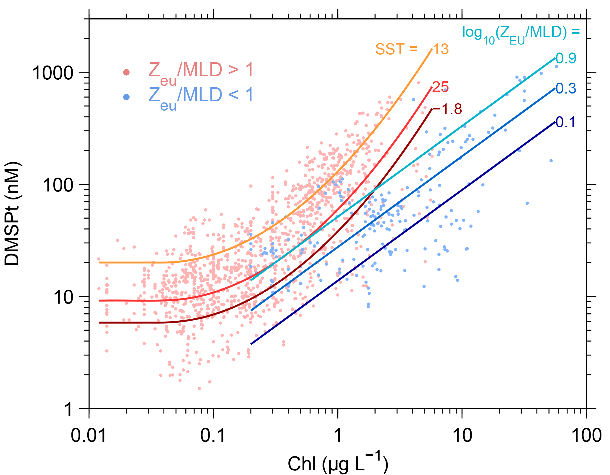
Figure A1DMSPtSAT sub-algorithm. Dots in the background show database measurements, and lines represent fits for “stratified” and “mixed” conditions at different SST and Zeu∕MLD ratios, respectively.
The supplement related to this article is available online at: https://doi.org/10.5194/bg-15-3497-2018-supplement.
MG designed the study, performed the research and wrote the paper, with input from all coauthors through the different phases. ED processed remote sensing reflectance data used as input for the Northern Hemisphere DMSSAT time series.
The authors declare that they have no conflict of interest.
We thank the NASA Ocean Biology Distributed Active Archive Center (OB.DAAC)
for access to MODIS and SeaWiFS datasets, Timothy (Tim) Bates (NOAA/PMEL) for
the maintenance of the GSS DMS(P) database and the DMS-GO project for the
recent database update (a joint initiative of the SOLAS Integration Project
and the EU projects COST Action 735 and EUR-OCEANS to Rafel Simó);
Eric Rehm and Maxime Benoît-Gagné for IT support; Naomi Levine,
John Dacey, Nick Bates and Scott Doney for sharing BATS data; and
Marie Robert and Michael Arychuk for guidance on access to Ocean Station P
public datasets. We acknowledge funding from the Canada Excellence Research
Chair in Remote Sensing of Canada's New Arctic Frontier (Marcel Babin), the
Canada Research Chair on Ocean Biogeochemistry and Climate, NSERC Discovery
Grant Program, Northern Research Supplement Program (Maurice Levasseur), the
NETCARE network (funded under the NSERC Climate Change and Atmospheric
Research program) and ArcticNet (The Network of Centres of Excellence of
Canada). Rafel Simó acknowledges funding from the Spanish Ministry of
Economy through project BIOGAPS. Martí Galí acknowledges the
receipt of a Beatriu de Pinós postdoctoral fellowship funded by AGAUR
(Generalitat de Catalunya). This project is a contribution to the research
program of Québec-Océan and the Takuvik Joint International
Laboratory (CNRS-France and Univeristé
Laval-Canada).
Edited by: S. Wajih A.
Naqvi
Reviewed by: two anonymous referees
Alcolombri, U., Ben-Dor, S., Feldmesser, E., Levin, Y., Tawfik, D. S., and Vardi, A.: Identification of the algal dimethyl sulfide-releasing enzyme: A missing link in the marine sulfur cycle, Science, 348, 1466–1469, 2015.
Archer, S. D., Cummings, D., Llewellyn, C., and Fishwick, J.: Phytoplankton taxa, irradiance and nutrient availability determine the seasonal cycle of DMSP in temperate shelf seas, Mar. Ecol.-Prog. Ser., 394, 111–124, https://doi.org/10.3354/meps08284, 2009.
Archer, S. D., Ragni, M., Webster, R., Airs, R. L., and Geider, R. J.: Dimethyl sulfoniopropionate and dimethyl sulfide production in response to photoinhibition in Emiliania huxleyi, Limnol. Oceanogr., 55, 1579–1589, https://doi.org/10.4319/lo.2010.55.4.1579, 2010.
Asher, E., Dacey, J. W., Ianson, D., Peña, M. A., and Tortell, P. D.: Concentrations and cycling of DMS, DMSP, and DMSO in coastal and offshore waters of the Subarctic Pacific during summer, 2010–2011, J. Geophys. Res.-Oceans, 119, 7123–7138, https://doi.org/10.1002/2014JC010066, 2017.
Bailey, K. E., Toole, D. A., Blomquist, B., Najjar, R. G., Huebert, B., Kieber, D. J., Kiene, R. P., Matrai, P., Westby, G. R., and del Valle, D. A.: Dimethylsulfide production in Sargasso Sea eddies, Deep-Sea Res. Pt. II, 55, 1491–1504, https://doi.org/10.1016/j.dsr2.2008.02.011, 2008.
Belviso, S., Masotti, I., Tagliabue, A., Bopp, L., Brockmann, P., Fichot, C., Caniaux, G., Prieur, L., Ras, J., Uitz, J., Loisel, H., Dessailly, D., Alvain, S., Kasamatsu, N., and Fukuchi, M.: DMS dynamics in the most oligotrophic subtropical zones of the global ocean, Biogeochemistry, 110, 215–241, https://doi.org/10.1007/s10533-011-9648-1, 2012.
Brainerd, K. E. and Gregg, M. C.: Surface mixed and mixing layer depths, Deep-Sea Res. Pt. I, 42, 1521–1543, 1995.
Brooks, S. D. and Thornton, D. C. O.: Marine Aerosols and Clouds, Annu. Rev. Mar. Sci., 10, 289–313, 2018.
Carpenter, L. J., Archer, S. D., and Beale, R.: Ocean–atmosphere trace gas exchange, Chem. Soc. Rev., 41, 6473–6505, https://doi.org/10.1039/c2cs35121h, 2012.
Carslaw, K. S., Lee, L. A., Reddington, C. L., Pringle, K. J., Rap, A., Forster, P. M., Mann, G. W., Spracklen, D. V., Woodhouse, M. T., Regayre, L. A., and Pierce, J. R.: Large contribution of natural aerosols to uncertainty in indirect forcing, Nature, 503, 67–71, https://doi.org/10.1038/nature12674, 2013.
Charlson, R. J., Lovelock, J. E., Andreae, M. O., and Warren, S. G.: Oceanic phytoplankton, atmospheric sulphur, cloud albedo and climate, Nature, 326, 655–661, 1987.
Curson, A. R. J., Todd, J. D., Sullivan, M. J., and Johnston, A. W. B.: Catabolism of dimethylsulphoniopropionate: microorganisms, enzymes and genes, Nat. Rev. Microbiol., 9, 849–859, https://doi.org/10.1038/nrmicro2653, 2011.
Le Clainche, Y., Vézina, A., Levasseur, M., Cropp, R. A., Gunson, J. R., Vallina, S. M., Vogt, M., Lancelot, C., Allen, J. I., Archer, S. D., Bopp, L., Deal, C., Elliott, S., Jin, M., Malin, G., Schoemann, V., Simó, R., Six, K. D., and Stefels, J.: A first appraisal of prognostic ocean DMS models and prospects for their use in climate models, Global Biogeochem. Cy., 24, GB3021, https://doi.org/10.1029/2009GB003721, 2010.
Devred, E., Sathyendranath, S., and Platt, T.: Delineation of ecological provinces using ocean colour radiometry, Mar. Ecol.-Prog. Ser., 346, 1–13, https://doi.org/10.3354/meps07149, 2007.
Frouin, R., Franz, B., and Wang, M.: Algorithm to estimate PAR from SeaWiFS data Version 1.2-Documentation, NASA (National Aeronautics and Space Administration), Washington DC, USA, 2003.
Gabric, A. J., Matrai, P. a., Kiene, R. P., Cropp, R., Dacey, J. W. H., DiTullio, G. R., Najjar, R. G., Simó, R., Toole, D. A., and DelValle, D. a.: Factors determining the vertical profile of dimethylsulfide in the Sargasso Sea during summer, Deep-Sea Res. Pt. II, 55, 1505–1518, https://doi.org/10.1016/j.dsr2.2008.02.002, 2008.
Galí, M. and Simó, R.: Occurrence and cycling of dimethylated sulfur compounds in the Arctic during summer receding of the ice edge, Mar. Chem., 122, 105–117, https://doi.org/10.1016/j.marchem.2010.07.003, 2010.
Galí, M. and Simó, R.: A meta-analysis of oceanic DMS and DMSP cycling processes: Disentangling the summer paradox, Global Biogeochem. Cy., 29, 496–515, https://doi.org/10.1002/2014GB004940, 2015.
Galí, M., Simó, R., Vila-Costa, M., Ruiz-González, C., Gasol, J. M., and Matrai, P. A.: Diel patterns of oceanic dimethylsulfide (DMS) cycling: Microbial and physical drivers, Global Biogeochem. Cy., 27, 620–636, 2013.
Galí, M., Devred, E., Levasseur, M., Royer, S.-J., and Babin, M.: A remote sensing algorithm for planktonic dimethylsulfoniopropionate (DMSP) and an analysis of global patterns, Remote Sens. Environ., 171, 171–184, https://doi.org/10.1016/j.rse.2015.10.012, 2015.
Grandey, B. S. and Wang, C.: Enhanced marine sulphur emissions offset global warming and impact rainfall, Sci. Rep., 5, 13055, https://doi.org/10.1038/srep13055, 2015.
Halloran, P. R., Bell, T. G., and Totterdell, I. J.: Can we trust empirical marine DMS parameterisations within projections of future climate?, Biogeosciences, 7, 1645–1656, https://doi.org/10.5194/bg-7-1645-2010, 2010.
Harrison, P. J., Whitney, F. A., Tsuda, A., Saito, H., and Tadokoro, K.: Nutrient and plankton dynamics in the NE and NW Gyres of the subarctic Pacific Ocean, J. Oceanogr., 60, 93–117, https://doi.org/10.1023/B:JOCE.0000038321.57391.2a, 2004.
Humphries, G. R. W., Deal, C. J., Elliott, S., and Huettmann, F.: Spatial predictions of sea surface dimethylsulfide concentrations in the high arctic, Biogeochemistry, 110, 287–301, https://doi.org/10.1007/s10533-011-9683-y, 2012.
Jarníková, T. and Tortell, P. D.: Towards a revised climatology of summertime dimethylsulfide concentrations and sea–air fluxes in the Southern Ocean, Environ. Chem., 13, 364–378, https://doi.org/10.1071/EN14272, 2016.
Johnson, R., Strutton, P. G., Wright, S. W., McMinn, A., and Meiners, K. M.: Three improved satellite chlorophyll algorithms for the Southern Ocean, J. Geophys. Res.-Oceans, 118, 3694–3703, https://doi.org/10.1002/jgrc.20270, 2013.
Jolliff, J. K., Kindle, J. C., Shulman, I., Penta, B., Friedrichs, M. A. M., Helber, R., and Arnone, R. A.: Summary diagrams for coupled hydrodynamic-ecosystem model skill assessment, J. Marine Syst., 76, 64–82, https://doi.org/10.1016/j.jmarsys.2008.05.014, 2009.
Jodwalis, C. M. and Benner, R. L.: On the possibility of remotely sensing global dimethyl sulfide sea-to-air flux, Polar Rec. (Gr. Brit)., 31, 251–256, 1995.
Kameyama, S., Tanimoto, H., Inomata, S., Yoshikawa-Inoue, H., Tsunogai, U., Tsuda, A., Uematsu, M., Ishii, M., Sasano, D., Suzuki, K., and Nosaka, Y.: Strong relationship between dimethyl sulfide and net community production in the western subarctic Pacific, Geophys. Res. Lett., 40, 3986–3990, https://doi.org/10.1002/grl.50654, 2013.
Kettle, A. J. and Andreae, M. O.: Flux of dimethylsulfide from the oceans: A comparison of updated data sets and flux models, J. Geophys. Res., 105, 26793, https://doi.org/10.1029/2000JD900252, 2000.
Kettle, A. J., Andreae, T. W., Amouroux, D., Bates, T. S., Berresheim, H., Bingemer, H., Boniforti, R., Helas, G., Leck, C., Maspero, M., Matrai, P., McTaggart, A. R., Mihalopoulos, N., Nguyen, B. C., Novo, A., Putaud, J. P., Rapsomanikis, S., Roberts, G., Schebeske, G., Sharma, S., Simó, R., Staubes, R., Turner, S., and Uher, G.: A global data base of sea surface dimethylsulfide (DMS) measurements and a simple model to predict sea surface DMS as a function of latitude, longitude, and month, Global Biogeochem. Cy., 13, 399–444, https://doi.org/10.1029/1999GB900004, 1999.
Kirk, J. T. O.: Light and photosynthesis in aquatic ecosystems, Cambridge, New York, NY, 2011.
Krüger, O. and Grabßl, H.: Southern Ocean phytoplankton increases cloud albedo and reduces precipitation, Geophys. Res. Lett., 38, 1–5, https://doi.org/10.1029/2011GL047116, 2011.
Kulmala, M., Petäjä, T., Ehn, M., Thornton, J., Sipilä, M., Worsnop, D. R., and Kerminen, V.-M.: Chemistry of atmospheric nucleation: on the recent advances on precursor characterization and atmospheric cluster composition in connection with atmospheric new particle formation, Annu. Rev. Phys. Chem., 65, 21–37, https://doi.org/10.1146/annurev-physchem-040412-110014, 2014.
Lana, A., Bell, T. G., Simó, R., Vallina, S. M., Ballabrera-Poy, J., Kettle, A. J., Dachs, J., Bopp, L., Saltzman, E. S., Stefels, J., Johnson, J. E., and Liss, P. S.: An updated climatology of surface dimethlysulfide concentrations and emission fluxes in the global ocean, Global Biogeochem. Cy., 25, GB1004, https://doi.org/10.1029/2010GB003850, 2011.
Lavoie, M., Levasseur, M., and Sunda, W. G.: A steady-state physiological model for intracellular dimethylsulfoxide in marine phytoplankton, Environ. Chem., 13, 212–219, https://doi.org/10.1071/EN14221, 2015.
Leaitch, W. R., Sharma, S., Huang, L., Toom-Sauntry, D., Chivulescu, A., Macdonald, A. M., von Salzen, K., Pierce, J. R., Bertram, A. K., Schroder, J. C., Shantz, N. C., Chang, R. Y. W., and Norman, A.-L.: Dimethyl sulfide control of the clean summertime Arctic aerosol and cloud, Elem. Sci. Anth., 1, 17, https://doi.org/10.12952/journal.elementa.000017, 2013.
Lee, Z., Weidemann, A., Kindle, J., Arnone, R., Carder, K. L., and Davis, C.: Euphotic zone depth: Its derivation and implication to ocean-color remote sensing, J. Geophys. Res., 112, C03009, https://doi.org/10.1029/2006JC003802, 2007.
Levasseur, M.: Impact of Arctic meltdown on the microbial cycling of sulphur, Nat. Geosci., 6, 691–700, https://doi.org/10.1038/ngeo1910, 2013.
Levasseur, M., Scarratt, M., Michaud, S., Merzouk, A., Wong, C., Arychuk, M., Richardson, W., Rivkin, R., Hale, M., and Wong, S.: DMSP and DMS dynamics during a mesoscale iron fertilization experiment in the Northeast Pacific – Part I: Temporal and vertical distributions, Deep-Sea Res. Pt. II, 53, 2353–2369, https://doi.org/10.1016/j.dsr2.2006.05.023, 2006.
Levine, N. M., Toole, D. A., Neeley, A., Bates, N. R., Doney, S. C., and Dacey, J. W. H.: Revising upper-ocean sulfur dynamics near Bermuda: New lessons from 3 years of concentration and rate measurements, Environ. Chem., 13, 302–313, https://doi.org/10.1071/EN15045, 2016.
Lizotte, M., Levasseur, M., Michaud, S., Scarratt, M. G., Merzouk, A., Gosselin, M., Pommier, J., Rivkin, R. B., and Kiene, R. P.: Macroscale patterns of the biological cycling of dimethylsulfoniopropionate (DMSP) and dimethylsulfide (DMS) in the Northwest Atlantic, Biogeochemistry, 110, 183–200, https://doi.org/10.1007/s10533-011-9698-4, 2012.
Longhurst, A.: Ecological Geography of the Sea, 2nd Edn., Academic Press, Amsterdam, Boston, Heidelberg, 2010.
Mahajan, A. S., Fadnavis, S., Thomas, M. A., Pozzoli, L., Gupta, S., Royer, S., Saiz-lopez, A., and Simó, R.: Quantifying the impacts of an updated global dimethylsulfide climatology on cloud microphysics and aerosol radiative forcing, J. Geophys. Res.-Atmos., 120, 2524–2536, https://doi.org/10.1002/2014JD022687, 2015.
Maritorena, S., Siegel, D. A., and Peterson, A. R.: Optimization of a semianalytical ocean color model for global-scale applications, Appl. Optics, 41, 2705–2714, https://doi.org/10.1364/AO.41.002705, 2002.
McCoy, D. T., Burrows, S. M., Wood, R., Grosvenor, D. P., Elliott, S. M., Ma, P., Rasch, P. J., and Hartmann, D. L.: Natural aerosols explain seasonal and spatial patterns of Southern Ocean cloud albedo, Sci. Adv., 1, e1500157, https://doi.org/10.1126/sciadv.1500157, 2015.
Merzouk, A., Levasseur, M., Scarratt, M., Michaud, S., Rivkin, R., Hale, M., Kiene, R. P., Price, N., and Li, W.: DMSP and DMS dynamics during a mesoscale iron fertilization experiment in the Northeast Pacific–Part II: Biological cycling, Deep-Sea Res. Pt. II, 53, 2370–2383, https://doi.org/10.1016/j.dsr2.2006.05.022, 2006.
Meskhidze, N. and Nenes, A.: Phytoplankton and cloudiness in the Southern Ocean, Science, 314, 1419–23, https://doi.org/10.1126/science.1131779, 2006.
Modini, R. L., Ristovski, Z. D., Johnson, G. R., He, C., Surawski, N., Morawska, L., Suni, T., and Kulmala, M.: New particle formation and growth at a remote, sub-tropical coastal location, Atmos. Chem. Phys., 9, 7607–7621, https://doi.org/10.5194/acp-9-7607-2009, 2009.
Mopper, K., Kieber, D. J., and Stubbins, A.: Marine Photochemistry of Organic Matter: Processes and Impacts, in: Biogeochemistry of Marine Dissolved Organic Matter, edited by: Hansell, D. A. and Carlson, C. A., Academic Press, Amsterdam, Boston, Heidelberg, 389–450, 2015.
Morel, A. and Smith, R. C.: Relation between total quanta and total energy for aquatic photosynthesis, Limnol. Oceanogr., 19, 591–600, 1974.
Nemcek, N., Ianson, D., and Tortell, P. D.: A high-resolution survey of DMS, CO2, and O2 ∕ Ar distributions in productive coastal waters, Global Biogeochem. Cy., 22, 1–13, https://doi.org/10.1029/2006GB002879, 2008.
Park, K.-T., Jang, S., Lee, K., Yoon, Y. J., Kim, M.-S., Park, K., Cho, H.-J., Kang, J.-H., Udisti, R., Lee, B.-Y., and Shin, K.-H.: Observational evidence for the formation of DMS-derived aerosols during Arctic phytoplankton blooms, Atmos. Chem. Phys., 17, 9665–9675, https://doi.org/10.5194/acp-17-9665-2017, 2017.
Polimene, L., Archer, S. D., Butenschön, M., and Allen, J. I.: A mechanistic explanation of the Sargasso Sea DMS “summer paradox”, Biogeochemistry, 110, 243–255, https://doi.org/10.1007/s10533-011-9674-z, 2011.
Quinn, P. K. and Bates, T. S.: The case against climate regulation via oceanic phytoplankton sulphur emissions, Nature, 480, 51–56, https://doi.org/10.1038/nature10580, 2011.
Quinn, P. K., Coffman, D. J., Johnson, J. E., Upchurch, L. M., and Bates, T. S.: Small fraction of marine cloud condensation nuclei made up of sea spray aerosol, Nat. Geosci., 10, 674–679, https://doi.org/10.1038/ngeo3003, 2017.
Royer, S.-J., Levasseur, M., Lizotte, M., Arychuk, M., Scarratt, M. G., Wong, C., Lovejoy, C., Robert, M., Johnson, K., Pena, A., Michaud, S., and Kiene, R. P.: Microbial dimethylsulfoniopropionate (DMSP) dynamics along a natural iron gradient in the northeast subarctic Pacific, Limnol. Oceanogr., 55, 1614–1626, https://doi.org/10.4319/lo.2010.55.4.1614, 2010.
Royer, S. J., Galí, M., Saltzman, E. S., McCormick, C. A., Bell, T. G., and Simó, R.: Development and validation of a shipboard system for measuring high-resolution vertical profiles of aqueous dimethylsulfide concentrations using chemical ionisation mass spectrometry, Environ. Chem., 11, 309–317, https://doi.org/10.1071/EN13203, 2014.
Royer, S., Mahajan, A. S., Galí, M., Saltzman, E., and Simó, R.: Small-scale variability patterns of DMS and phytoplankton in surface waters of the tropical and subtropical Atlantic, Indian, and Pacific Oceans, Geophys. Res. Lett., 42, 475–483, https://doi.org/10.1002/2014GL062543, 2015.
Royer, S.-J., Galí, M., Mahajan, A. S., Ross, O. N., Pérez, G. L., Saltzman, E. S., and Simó, R.: A high-resolution time-depth view of dimethylsulphide cycling in the surface sea, Sci. Rep., 6, srep32325, https://doi.org/10.1038/srep32325, 2016.
Sanchez, K. J., Chen, C. L., Russell, L. M., Betha, R., Liu, J., Price, D. J., Massoli, P., Ziemba, L. D., Crosbie, E. C., Moore, R. H., Müller, M., Schiller, S. A., Wisthaler, A., Lee, A. K. Y., Quinn, P. K., Bates, T. S., Porter, J., Bell, T. G., Saltzman, E. S., Vaillancourt, R. D., and Behrenfeld, M. J.: Substantial Seasonal Contribution of Observed Biogenic Sulfate Particles to Cloud Condensation Nuclei, Sci. Rep., 8, 1–14, https://doi.org/10.1038/s41598-018-21590-9, 2018.
Schlesinger, W. H. and Bernhardt, E. S.: The Global Cycles of Sulfur and Mercury, in Biogeochemistry. An Analysis of Global Change, 3rd Edn., 469–486, https://doi.org/10.1016/B978-0-12-385874-0.00012-1, Academic Press, 2013.
Schmidtko, S., Johnson, G. C., and Lyman, J. M.: MIMOC: A global monthly isopycnal upper-ocean climatology with mixed layers, J. Geophys. Res.-Oceans, 118, 1658–1672, https://doi.org/10.1002/jgrc.20122, 2013.
Shaw, G. E.: Bio-controlled thermostasis involving the sulfur cycle, Clim. Change, 5, 297–303, https://doi.org/10.1007/BF02423524, 1983.
Simó, R.: From cells to globe?: approaching the dynamics of DMS(P) in the ocean at multiple scales, Can. J. Fish. Aquat. Sci., 61, 673–684, https://doi.org/10.1139/F04-030, 2004.
Simó, R.: The role of marine microbiota in short-term climate regulation, in: The Role of Marine Biota in the Functioning of the Biosphere, edited by: Duarte, C. M., Fundación BBVA, Bilbao, Spain, 107–130, 2011.
Simó, R. and Dachs, J.: Global ocean emission of dimethylsulfide predicted from biogeophysical data, Global Biogeochem. Cy., 16, 1078, https://doi.org/10.1029/2001GB001829, 2002.
Simó, R. and Pedrós-Alió, C.: Role of vertical mixing in controlling the oceanic production of dimethyl sulphide, Nature, 402, 396–399, 1999.
Stefels, J.: Physiological aspects of the production and conversion of DMSP in marine algae and higher plants, J. Sea Res., 43, 183–197, https://doi.org/10.1016/S1385-1101(00)00030-7, 2000.
Stefels, J., Steinke, M., Turner, S. M., Malin, G., and Belviso, S.: Environmental constraints on the production and removal of the climatically active gas dimethylsulphide (DMS) and implications for ecosystem modelling, Biogeochemistry, 83, 245–275, 2007.
Steiner, N. S., Robert, M., Arychuk, M., Levasseur, M. L., Merzouk, A., Peña, M. A., Richardson, W. A., and Tortell, P. D.: Evaluating DMS measurements and model results in the Northeast subarctic Pacific from 1996–2010, Biogeochemistry, 110, 269–285, https://doi.org/10.1007/s10533-011-9669-9, 2012.
Sunda, W., Kieber, D. J., Kiene, R. P., and Huntsman, S.: An antioxidant function for DMSP and DMS in marine algae, Nature, 418, 317–320, https://doi.org/10.1038/nature00851, 2002.
Sunda, W. G., Hardison, R., Kiene, R. P., Bucciarelli, E., and Harada, H.: The effect of nitrogen limitation on cellular DMSP and DMS release in marine phytoplankton: climate feedback implications, Aquat. Sci., 69, 341–351, https://doi.org/10.1007/s00027-007-0887-0, 2007.
Sutherland, G., Reverdin, G., Marié, L., and Ward, B.: Mixed and mixing layer depths in the ocean surface boundary, Geophys. Res. Lett., 41, 8469–8476, https://doi.org/10.1002/2014GL061939, 2014.
Tesdal, J.-E., Christian, J. R., Monahan, A. H., and von Salzen, K.: Evaluation of diverse approaches for estimating sea-surface DMS concentration and air–sea exchange at global scale, Environ. Chem., 13, 390–412, https://doi.org/10.1071/EN14255, 2016.
Thompson, A. M., Esaias, W. E., and Iverson, R. L.: Two Approaches to Determining the Sea-to-Air Flux of Dimethyl Sulfide: Satellite Ocean Color and a Photochemical Model With Atmospheric Measurements, J. Geophys. Res., 95, 20551–20558, 1990.
Toole, D. A. and Siegel, D. A.: Light-driven cycling of dimethylsulfide (DMS) in the Sargasso Sea: Closing the loop, Geophys. Res. Lett., 31, 5–8, https://doi.org/10.1029/2004GL019581, 2004.
Vallina, S. M. and Simó, R.: Re-visiting the CLAW hypothesis, Environ. Chem., 4, 384–387, https://doi.org/10.1071/EN07055, 2007a.
Vallina, S. M. and Simó, R.: Strong relationship between DMS and the solar radiation dose over the global surface ocean, Science, 315, 506–508, https://doi.org/10.1126/science.1133680, 2007b.
Vallina, S. M., Simó, R., and Manizza, M.: Weak response of oceanic dimethylsulfide to upper mixing shoaling induced by global warming, P. Natl. Acad. Sci. USA, 104, 16004–16009, https://doi.org/10.1073/pnas.0700843104, 2007.
Vallina, S. M., Simó, R., Anderson, T. R., Gabric, A., Cropp, R., and Pacheco, J. M.: A dynamic model of oceanic sulfur (DMOS) applied to the Sargasso Sea: Simulating the dimethylsulfide (DMS) summer paradox, J. Geophys. Res., 113, 1–23, https://doi.org/10.1029/2007JG000415, 2008.
Vantrepotte, V. and Mélin, F.: Inter-annual variations in the SeaWiFS global chlorophyll a concentration (1997–2007), Deep-Sea Res. Pt. I, 58, 429–441, https://doi.org/10.1016/j.dsr.2011.02.003, 2011.
Vila-Costa, M., Kiene, R. P., and Simó, R.: Seasonal variability of the dynamics of dimethylated sulfur compounds in a coastal northwest Mediterranean site, Limnol. Oceanogr., 53, 198–211, 2008.
Yu, F. and Luo, G.: Oceanic dimethyl sulfide emission and new particle formation around the coast of antarctica: A modeling study of seasonal variations and comparison with measurements, Atmosphere, 1, 34–50, https://doi.org/10.3390/atmos1010034, 2010.