2.1 The Swedish forest and soil inventories (national database)

We combined a Swedish forest soil (Olsson, 1999; Lundin, 2011) and inventory database for the period 2003–2012 (Lundin, 2011) with a database for soil texture and climate information across Sweden. Precipitation data were extracted from the European Commission Joint Research Centre Monitoring Agricultural Resources dataset (EC–JRC–MARS, based on ECMWF model outputs and a reanalysis of ERA-Interim; see http://spirits.jrc.ec.europa.eu/; last access: 7 June 2018) based on the geographic location of each site. The dataset's spatial resolution is 0.25^∘ and averages were calculated for the period 1989–2012. The resulting data collection thus incorporated information on location, climate, soil, and vegetation for about 2500 forested plots (n= 1099 for spruce, n= 1422 for pine) spread over Sweden (Table 1).

Many of the (mostly managed) forest plots were not monocultures, but contained both Norway spruce (Picea abies (L.) H. Karst.) and Scots (or lodgepole) pine (Pinus sylvestris L. or Pinus contorta Douglas) trees, as well as other species. In order to contrast spruce and pine forests, we classified forests with ≥50 % basal area of spruce (pine) trees as spruce (pine). To quantify the influence of climate on productivity across Sweden (Question 1), we first determined the annual growing season temperature sum (TSUM) following a recently reparameterized version of the equation given in Odin et al. (1983), available on https://www.skogskunskap.se/; last access: 7 June 2018.

In order to facilitate comparisons among sites and to allow the calculation of the nutrient availability metric, we converted the soil measurements (SOC, soil texture, TEB, pH_w, pH_KCl, total nitrogen concentration (TN), and soil C : N ratio) taken per horizon to values representative of the upper 10 cm (i.e., the 0–10 cm layer) and the upper 20 cm (i.e., the 0–20 cm layer) of the soil, including the organic layer. To this end, we first calculated bulk densities (BDs) as

for the organic horizons and

for the mineral soil (Nilsson and Lundin, 2006).

Conversions of soil data (“variables”) per horizon to data per depth interval (layer x–y cm) were then performed as follows (soil mass per m² (kg m⁻²) = BD (kg m⁻³) ⋅ thickness_{horizon or layer} (m)):

The IIASA metric of constraints on nutrient availability, originally meant for use on arable land, incorporates four crop-specific scores (estimated for SOC, soil texture, TEB, and pH_w) that can be assigned to a soil (IIASA and FAO, 2012). These scores, which can be found in lookup tables (http://webarchive.iiasa.ac.at/Research/LUC/GAEZv3.0/soil_evaluation.html; last access: 7 June 2018), were derived from crop growth data on different agricultural soils. Given that we consider boreal forests and not crops, we averaged the scores of the different crop species for each of the four soil properties. We thus removed crop-specific requirements, but generally known relationships between the soil variables and plant performance (not only valid for agroecosystems), such as an optimum for pH, remained. In addition, we replaced the lookup-table-derived step functions with continuous empirical formulas to facilitate their calculation as well as their modification (Fig. 1):

The total score for nutrient availability, which can be interpreted as the expected actual yield (i.e., aboveground productivity) proportional to the maximum attainable yield (i.e., without nutrient constraints), was then calculated as follows (IIASA and FAO, 2012):

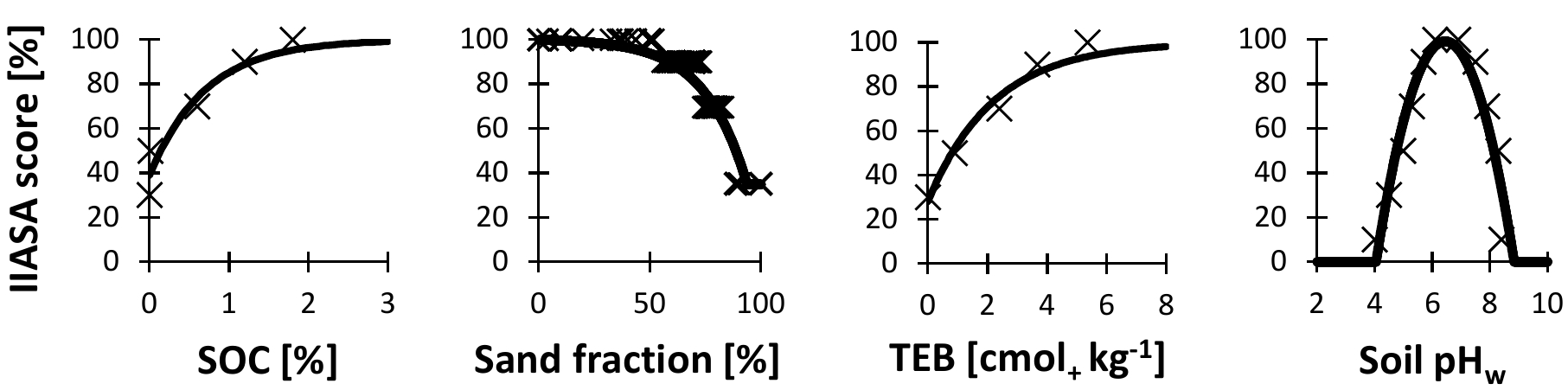
Figure 1IIASA soil scores for soil organic carbon concentration (SOC), texture, total exchangeable bases (TEB), and pH measured in water (pH_w). The curves were drawn based on approximate functions through the points, which were derived from crop-specific scores in a lookup table (http://webarchive.iiasa.ac.at/Research/LUC/GAEZv3.0/soil_evaluation.html; last access: 7 June 2018, IIASA and FAO, 2012) and averaged over all crop species in the table.

Download

Table 1Overview of variables of the database used in the current study. Each plot for soil and vegetation analyses had a 10 m radius and was sampled once during the period 2003–2012. The (mostly managed) forests in the inventory represent a random sample of Swedish forests. Abbreviations: MAP: mean annual precipitation; TSUM: growing season temperature sum; SOC: soil organic carbon concentration; TEB: total exchangeable bases; pH_w: pH measured in water; pH_KCl: pH measured in KCl solution; TN: total nitrogen concentration; soil C : N ratio: soil carbon-to-nitrogen ratio.

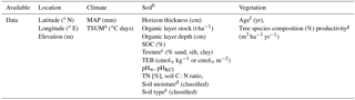
^a TSUM was calculated for each data point based on its latitude, longitude, and elevation. ^b n= 3; soil variables were determined using standard sampling and laboratory procedures (e.g., Olsson et al., 2009; Stendahl et al., 2010). ^c In an earlier version of the database, percentages of sand, silt, and clay were approximated from field-based soil texture class. ^d Soil moisture was determined in the field based on indicators (e.g., groundwater depth, moisture at the surface, ground vegetation, elevated tree trunks). The classification is representative of the average moisture conditions during the growing season (Olsson, 1999; Olsson et al., 2009). ^e Taxonomic soil classification is based on the World Reference Base for Soil Resources. ^f Stand age ranged between 1 and 350 years, with an average of 65 years. ^g Productivities (site quality) or mean annual volume increments (MAIs) over a full rotation were estimated based on height development curves. In situ productivities may be lower, depending on the management.

Download Print Version | Download XLSX

2.2 General approach

Forest productivity across Sweden depends not only on soil nutrient availability but also on climate, soil wetness, and N deposition. Before evaluating the metric, we removed the influence of climate on forest productivity (“PRE” in Fig. 2). The influence of soil moisture and N deposition are considered in further analyses (see Sect. 2.3.1). Normalized productivity was calculated in two alternative ways: (1) as the residuals of the regression model (of PRE; from here on referred to as “method 1”; Figs. 3a and S1a, b, Tables S1 and S2, and Eq. S1) and (2) as the ratio of the original productivity relative to the theoretical maximum productivity (from here on referred to as “method 2”; Figs. 3b and S1b, c). This theoretical maximum productivity, which was extracted from a map provided by Bergh et al. (2005) with ArcGIS (ESRI, 2011), indicates the productivity that could be obtained under non-nutrient-limited conditions and is further referred to as attainable productivity. The second method is thus very similar to the IIASA approach (see Eq. 1), but because an estimate for attainable productivity was only available for spruce, it could only be applied for this species. The two alternative methods for normalizing productivity were used to verify the robustness of the analyses, and because each method has its own advantages and disadvantages. The main disadvantage of method 1 is that not only the direct influence of climate on productivity is removed but also its indirect effect through nutrient availability, so that only effects of regional variation in nutrient availability on productivity remain. Method 2, however, involves an extrapolation based on the results of only a few fertilization experiments and thus comes with high uncertainty on the estimates of attainable productivity.

Regression analysis was then used to elucidate how the different soil variables were related to normalized productivity (Question 1). In addition, normalized productivity was fitted against the IIASA metric to test its performance. The correlation between the residuals of this relationship and each of the four variables of the metric then indicated whether or not the variables were well implemented (Question 2). Finally, the associations found in Question 1 indicated how the metric could be adjusted (Question 3). Two adjusted metrics were then evaluated in the same way as the original IIASA metric in Question 2, and by investigating if they could explain variation in productivity for five local gradients in nutrient availability. An overview of the methodology is presented in Fig. 2.

2.3 Data analyses

As explained in the paragraphs above, productivity was normalized using two methods. Method 1 considers the residuals to reflect deviations in productivity imposed by spatial variation in nutrient availability and in the absence of climate effects. However, residuals deviated more strongly from zero towards the warmer south (Fig. 3a), thus causing heteroscedasticity and a potential bias in the further analyses if not properly accounted for. For further analyses, we therefore split the database into three TSUM groups (north, middle, and south; Fig. 3a). For method 2, considering the ratio of actual to attainable productivity, this separation of different regions was not required.

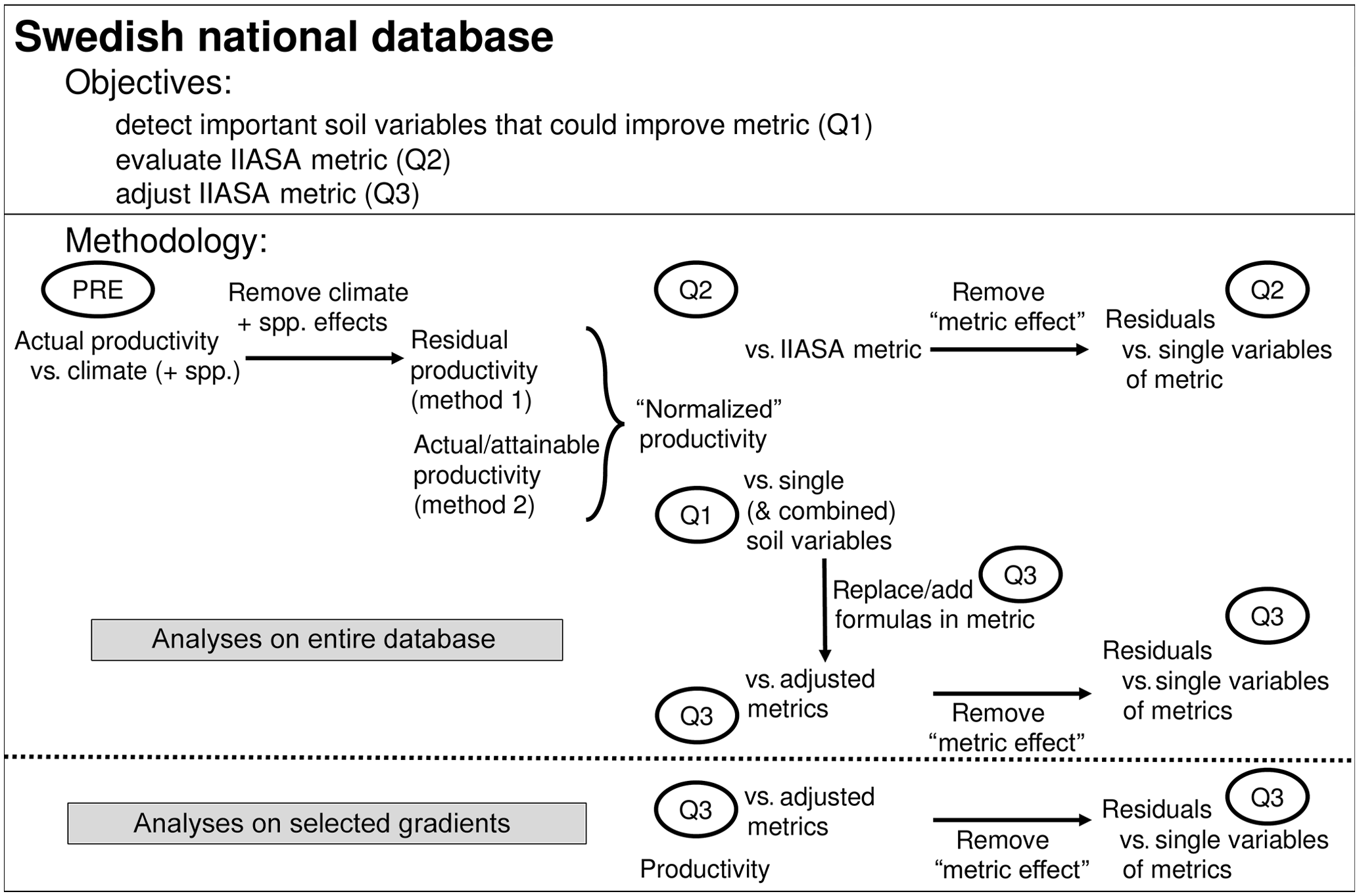
Figure 2Objectives and methods followed in the current paper. PRE refers to a regression model of productivity vs. climate and species (spp.); Question 1, Question 2, and Question 3 refer to the research questions. Performance of the adjusted nutrient metrics was evaluated against the entire database, and against five nutrient availability gradients, selected from the database (Fig. S2).

Download

2.3.2 Question 1 – normalized productivity vs. single and combined soil variables

Simple regression analysis was used to determine the relationship between single soil variables and normalized productivity. To test the robustness of the observed relationships in the absence of potentially confounding effects of soil moisture and type, we performed these analyses on all data, and on the data stratified by soil moisture and soil type. Then, we tested which combination of continuous soil variables best explained variation in normalized productivity across Sweden (multiple regression analysis). Starting from the full model containing all explanatory variables, the least significant term was removed, resulting in a simplified model. Performance of the full and simplified models was then compared using the mean squared error (mse), based on cross validation (package DAAG – Maindonald and Braun, 2015). We repeated this model simplification procedure until mse stopped decreasing. Interaction effects up to the first order were added if suggested by regression trees (package tree – Ripley, 2015). For method 1 (Fig. 3), first-order interactions of continuous variables with region as a factor (levels: N, M, S) were included in the selection procedure (i.e., an ANCOVA was used for this approach).

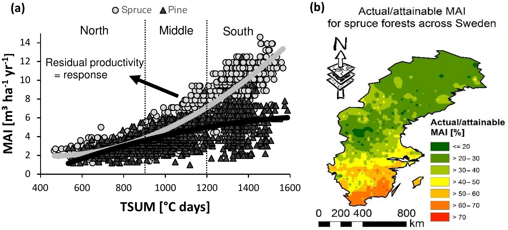
Figure 3Normalized productivity was calculated in two alternative ways. (a) In method 1, residual values were taken from a regression model, explaining variation in mean annual increments (MAIs) by climate (growing season temperature sum or TSUM and precipitation) and species. The selection procedure, equation, and parameter estimates are given in the Supplement (respectively Tables S1 and S2 and Eq. S1 in the Supplement). In order to avoid heteroscedasticity-induced artifacts, the dataset was split into northern (TSUM < 900 ^∘C days), middle (900 ^∘C days < TSUM < 1200 ^∘C days), and southern (TSUM > 1200 ^∘C days) regions for this approach. (b) In method 2, actual productivities for spruce were divided by theoretically attainable productivities, provided by Bergh et al. (2005).

Download

2.3.4 Question 3 – adjustments of the IIASA metric

Outcomes of Question 1 indicated which soil variables best explained variation in normalized productivity. This information was further used to (i) assess if the relationships for variables already included in the IIASA metric should be altered, (ii) remove soil variables from the metric if their empirical associations with normalized productivity were opposite from their relationships in the original IIASA metric, which would complicate parameterization, and (iii) include additional soil variables to improve performance of the metric. Two new metrics were developed: “adjusted metric 1” and “adjusted metric 2”, referring to the respective methods of normalizing productivity (Fig. 3). As a starting point for adjusted metric 1, half of the dataset from southern Sweden (where productivity varied most; see Fig 3a) was used as a calibration set to derive regression equations, while half of the complete national dataset for spruce served as a calibration set for adjusted metric 2. The best predictors of normalized productivity as indicated by the analyses in Question 1 were then adopted as partial metric scores (see the original Eqs. 6–9). Moreover, for adjusted metric 1, the minimum and maximum normalized productivities observed in southern Sweden were included as lower and upper boundaries to the partial metric scores to avoid possible unrealistic values for future applications to other datasets. For method 2, the minima and maxima were, as in the IIASA metric, set to 0 and 100 %, respectively (units for this metric (%) remained the same as in the original IIASA metric, while for new metric 1, the unit was (m³ ha⁻¹ yr⁻¹)). Finally, the two improved metrics for nutrient availability were calculated as in Eq. (10).

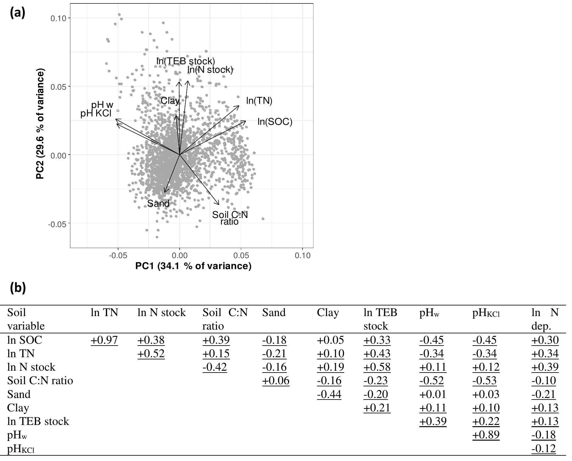
Figure 4Correlation structure of a set of potential key soil variables for a soil depth of 0–20 cm. Panel (a) shows the principal component analysis (PCA) biplot (SD for PC1 = 1.75, SD for PC2 = 1.63); panel (b) shows the correlation matrix, showing Pearson's r for the variable pairs, including correlations with nitrogen deposition. Underlined correlations were significant. Abbreviations: SOC: soil organic carbon concentration (%); TN: soil total nitrogen (%); N stock: amount of nitrogen in the layer (g m⁻²); Soil C : N ratio: soil carbon-to-nitrogen ratio; Sand: percentage of sand in the mineral soil; Clay: percentage of clay in the mineral soil; TEB: total exchangeable bases (cmol₊ m⁻²); pH_w: pH measured in water; pH_KCl: pH measured in KCl solution; N dep: nitrogen deposition.

Download

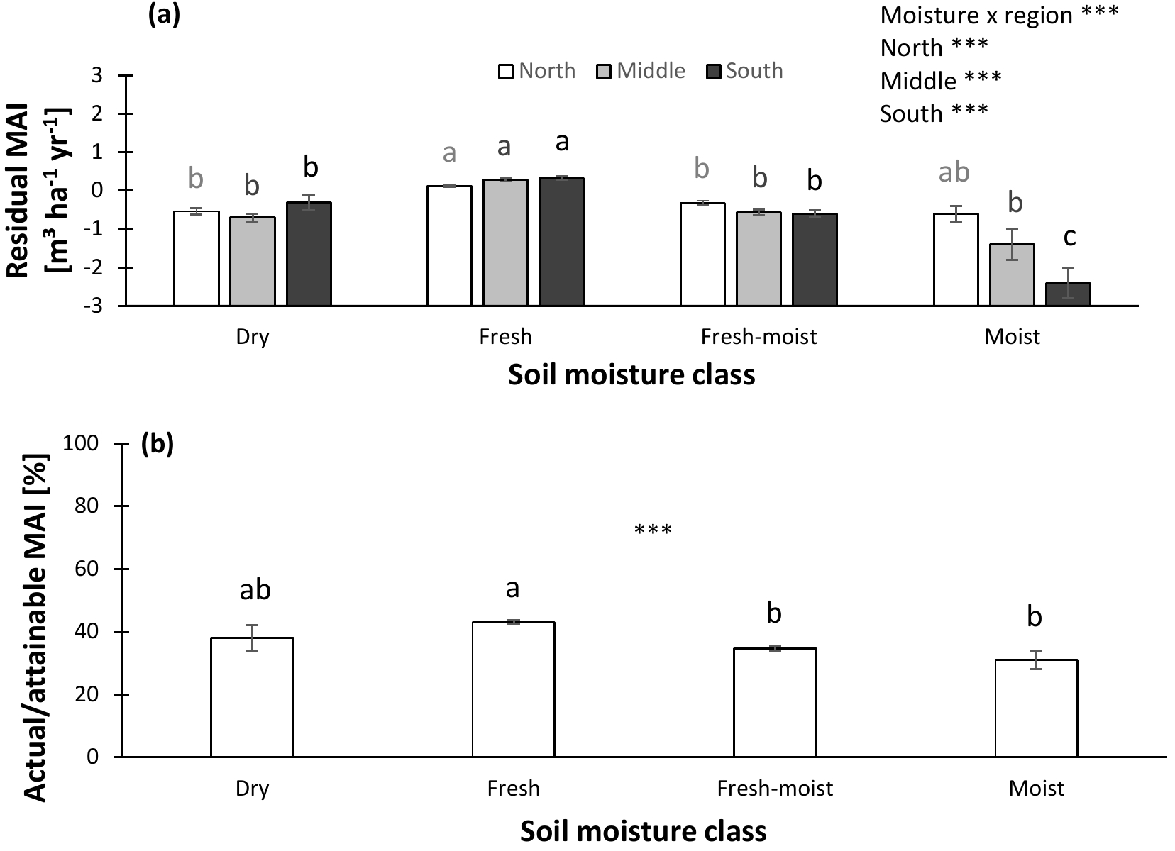
Figure 5Normalized productivity per soil moisture class. (a) Productivity normalized following method 1 (residual mean annual increment – MAI) vs. soil moisture. (b) Productivity normalized following method 2 (actual ∕ attainable mean annual increment – MAI) vs. soil moisture. In panel (a), separate analyses were performed for northern, middle, and southern Sweden, as the moisture effects differed among regions. ${}^{***}$ Indicates significant differences at the P < 0.01 level. Error bars represent the standard error of the mean (s.e.m).

Download

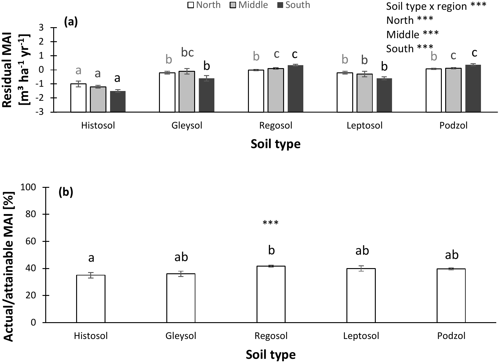
Figure 6Normalized productivity per soil type. (a) Productivity normalized following method 1 (residual mean annual increment – MAI) vs. soil type. (b) Productivity normalized following method 2 (actual ∕ attainable mean annual increment – MAI for spruce) vs. soil type. In panel (a), separate analyses were performed for northern, middle, and southern Sweden, as the soil type effects differed among regions. ${}^{***}$ Indicates significant differences at the P < 0.01 level. Error bars represent the s.e.m.

Download

Performance of the adjusted metrics was evaluated by (i) testing normalized productivity in the database against the metrics and inspecting the implementation of the variables, and by (ii) testing productivity against the metrics and examining variable implementation for five manually selected local gradients in nutrient availability. For (i), the metrics were thus evaluated as described for the IIASA metric under Question 2, with the exceptions that validation datasets were used (i.e., the data that were used for developing the metrics were not included for the evaluations) and that the same analyses were also performed after stratifying by soil moisture and type to assess robustness. For (ii), two gradients with spruce, and three gradients with pine (locations indicated in Fig. S2) were selected in ArcGIS (ESRI, 2011). Each of these gradients included at least 40 data points from the Swedish database that (i) were located in the same region, without showing substantial spatial variation in climate and (ii) showed high spatial variation in soil moisture, TEB, or productivity (we also searched specifically for clear soil C : N gradients, but found none for which climate did not vary; variables like soil C : N or SOC did however sufficiently vary within the five selected gradients: ≤ 16.8–≥ 32.2 and ≤ 1.6–≥ 48.5 %, respectively). We thus not only evaluated the adjusted metrics against normalized productivity across the complete database but also tested their performance for local gradients, which offered the advantage that no normalization of productivity for climate was needed.

We examined the validity of the linear models' assumptions (linearity, normality of residuals, no influential outliers, homoscedasticity) with standard functions of R (R Core Team, 2015), including diagnostic plots. Moreover, for all regressions, potential nonlinearities were detected with histograms of all variables' distributions and generalized additive models from the mgcv package (Wood, 2006). Data were log transformed if their distribution was right-skewed, while polynomial (e.g., quadratic) functions were included in the model selection procedure where the general additive models suggested nonlinear patterns. The variance inflation factor (package car – Fox and Weisberg, 2011) assessed possible multicollinearity. Whenever confidence intervals are given, they represent standard errors of the mean (s.e.m.). For all analyses, α= 0.05 was taken as the significance level, whereas P values between 0.05 and 0.10 were considered to be borderline significant.

3.1 Identifying potentially confounding factors

Correlations among soil properties and nutrients were investigated to verify if any of the variables could be excluded in the subsequent analyses due to redundancy. In this database, pH_w and pH_KCl were strongly correlated. As pH_KCl has the practical advantage of showing less seasonal variation than pH_w (Soil Survey Staff, 2014), we opted to use only pH_KCl in the analyses for research Question 1. Similarly, TN and SOC largely shared the same information. We included SOC in the analyses and discarded TN because SOC is a component of the IIASA metric of constraints on nutrient availability. Moreover, soil organic matter acts as a nutrient store and provides cation and anion exchange sites, while TN is merely correlated to SOM but only a (small) proportion of total N is available to the plants. Collinearity among other variables was minor ($\left|{\mathrm{Pearson}}^{\prime }\mathrm{s}r\right|\mathit{<}\mathrm{0.65}$; Fig. 4), and they were thus all included in the analysis.

Relationships between soil variables and normalized productivity might vary depending on factors such as soil moisture and soil type. Therefore, we first examined how these factors influence soil properties and normalized productivity. Soil moisture, for example, may influence nutrient availability of ecosystems by – among others – affecting the rate of decomposition, and consequently change other soil characteristics. In the database, each forest was originally assigned to a soil moisture category. Using these categories, we found that SOC and the soil C : N ratio increased from dry to moist. A similar trend was observed for TEB, while the sand fraction and pH_KCl decreased from dry to moist. For clay, no significant differences among soil moisture classes occurred (Fig. S3). Lastly, normalized productivity was highest in the fresh soil moisture class and lowest for the wettest forests (Fig. 5). This pattern was most pronounced in southern Sweden (north – $F_{\mathrm{3},\mathrm{568}}=$ 22.43, P < 0.01; middle – $F_{\mathrm{4},\mathrm{844}}=$ 39.47, P < 0.01; south – $F_{\mathrm{4},\mathrm{1056}}=$ 35.23, P < 0.01; moisture x region – $F_{\mathrm{7},\mathrm{2468}}=$ 3.77, P < 0.01).

Soil properties not only differed among soil moisture classes, but also among soil types. Especially Histosols and Podzols could be distinguished from the other soils: Histosols (which largely overlapped with the wet soil moisture classes) were characterized by a low pH_KCl and high SOC and soil C : N ratio, while Podzols were sandy and had a low TEB stock (Fig. S4). Differences in normalized productivity among soil types were observed as well. Histosols in particular showed reduced productivities compared to other soil types (Fig. 6). Hence, the wetness of a site and its type of soil (partly in parallel with wetness) could confound observed patterns in productivity associated with the soil variables and are therefore taken into account in further analyses and their interpretation.

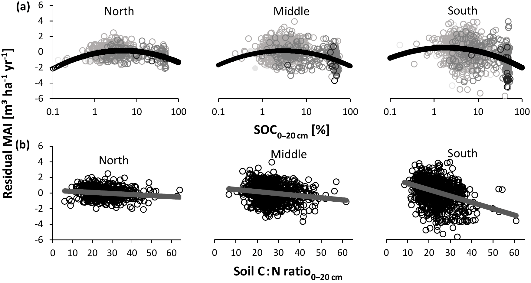
Figure 7Relationship between normalized productivity following method 1 (residual mean annual increment – MAI); (a) log-transformed soil organic carbon concentration (SOC); (b) soil carbon-to-nitrogen (C : N) ratio at a depth of 0–20 cm. Separate analyses were performed for northern, middle, and southern Sweden, as the SOC and C : N effects differed among regions. Point darkness in (a) represents soil moisture (darker: moister). Statistics corresponding to the panels are presented in Table 2. Note that the horizontal axis for SOC covers a broader range here than in Fig. 1, as SOC varied widely in the Swedish database.

Download

In addition to soil moisture and soil type, N deposition may also confound associations between normalized productivity and soil data. In our Swedish database, N deposition correlated significantly with all soil variables. Especially TN and SOC correlated positively with N deposition (Fig. 4b). N deposition was also strongly positively correlated with productivity (Pearson's r= 0.73); both variables increased from north to south, as did the growing season temperature sum (which was therefore also highly correlated with (ln) N deposition – Pearson's r= 0.91). However, N deposition did generally not have a significant effect on productivity normalized with method 1 (i.e., residual productivity), while with method 2 (i.e., actual ∕ attainable productivity), there was a strong positive relationship with N deposition. The increasing N deposition along the north–south gradient in Sweden (e.g., Olsson et al., 2009) should thus be kept in mind when interpreting effects of soil variables on productivity when normalized following method 2.

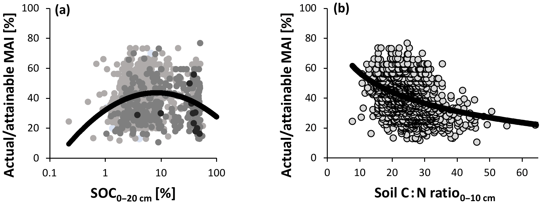
Figure 8Relationship between normalized productivity following method 2 (actual ∕ attainable mean annual increment – MAI for spruce); (a) log-transformed soil organic carbon concentration (SOC); (b) soil carbon-to-nitrogen ratio (C : N). Point darkness in (a) represents soil moisture (darker: moister). Statistics corresponding to the panels are presented in Table 2. Note that the horizontal axis for SOC covers a broader range here than in Fig. 1, as SOC varied widely in the Swedish database. Also note that the C : N ratio of the upper 10 cm was used instead of the upper 20 cm here, owing to a better description of variation in the response variable. Even though the C : N ratio roughly decreased southwards (Fig. S1d), it was only weakly correlated with the growing season temperature sum (r= −0.13 for C : N_0−20 cm and r= −0.28 for C : N_0−10 cm).

Download

Table 2Associations between single soil variables and normalized productivity for Swedish spruce and pine forests. Significance (P values) of single soil variable effects on residual productivity (mean annual increment – MAI (m³ ha⁻¹ yr⁻¹)) and actual ∕ attainable MAI (for spruce only) across Sweden are given. For (near) significant variables (i.e., P<0.10), parameter estimates ± s.e.m. and the proportion of variation explained (R²) are shown as well. Abbreviations: N: north; M: middle; S: south; SOC: soil organic carbon concentration; Soil C : N: soil carbon-to-nitrogen ratio; TEB: total exchangeable bases; quad: parameter estimate for quadratic term; lin: parameter estimate for linear term of a quadratic function. For actual ∕ attainable MAI, the model including 0–10 cm soil C : N performed better than the one with 0–20 cm soil C : N (ms = 173 vs. 159). No depths are given for soil texture (% sand and % clay) because these were previously calculated based on texture classes of the upper mineral soil with the help of particle size diagrams.

N/a: not applicable.

Download Print Version | Download XLSX

Table 3Estimates ± s.e.m. for parameters of the selected multiple regression equations linking soil variables to normalized productivity for Swedish conifer forests. Significance of the pattern (P values) and proportion of variation explained (R²) are given as well. Abbreviations: MAI: mean annual increment (m³ ha⁻¹ yr⁻¹); N: north; M: middle; S: south; SOC: soil organic carbon concentration; Soil C : N: soil carbon-to-nitrogen ratio; TEB: total exchangeable bases; quad: parameter estimate for quadratic term; lin: parameter estimate for linear term of a quadratic function. Output of the model selection procedures for methods 1 and 2 is shown in Tables S7 and S8. Data for method 1 are for both spruce and pine, whereas actual ∕ attainable MAI (method 2) was only available for spruce. No depths are given for soil texture (% sand) because these were previously calculated based on texture classes of the upper mineral soil with the help of particle size.

N/a: not applicable.

Download Print Version | Download XLSX

3.2 Question 1 – normalized productivity vs. single and combined soil variables

In order to elucidate how soil variables affect nutrient availabilities across Sweden, we used their single and combined relationships with normalized productivity. For method 1, we found that most single soil variables were significantly related to normalized productivity (Table 2; R² ranged between 0.002 and 0.146). For both SOC (Fig. 7a) and pH_KCl, the relationship with normalized productivity showed an optimum (i.e., an empirical quadratic relationship fit better than a linear model). Normalized productivity was significantly negatively correlated with the soil C : N ratio (Fig. 7b), for which the effect became more pronounced towards the south (i.e., slopes and R² values increased; F_2.2274= 34.23, P < 0.01). Finally, associations with soil N stocks and clay were weak (but significantly positive). The strongest relationships were found for normalized productivity versus SOC, pH_KCl, and soil C : N ratio and consequently these were among the variables selected for the model with multiple covariates (Table 3).

Results of method 2 were qualitatively similar to those of the other approach for SOC (Fig. 8a), N stock, soil C : N ratio (Fig. 8b), clay fraction, and TEB, although the N stock explained a larger proportion of the variation here and the curve for actual ∕ attainable productivity decreased logarithmically rather than linearly with increasing C : N ratio. However, the function for pH_KCl did not show an optimum, but was linear with a significantly positive slope (Table 2). In summary, SOC and the soil C : N ratio were the only soil factors that showed a similar trend, according both methods with an R² of at least a few percent, and were thus included in the multiple regression models for both methods 1 and 2 (these models also included other variables resulting from the stepwise regression analysis; Table 3).

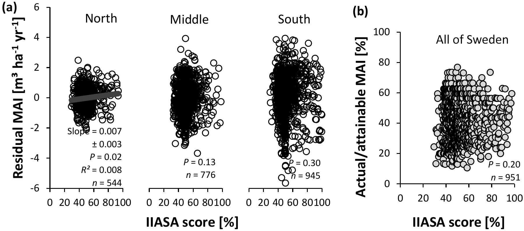
Figure 9Evaluation of the IIASA metric of constraints on nutrient availability for Swedish conifer forests. (a) Method 1 – association with residual mean annual increments (MAIs) of the productivity–climate regression model (Fig. 3a, Eq. S1 and Table S2), distinguishing northern, middle, and southern Sweden. (b) Method 2 – association with actual ∕ attainable MAI for the entire Swedish land area (Fig. 3b). Full line: significant slope (P < 0.05).

Download

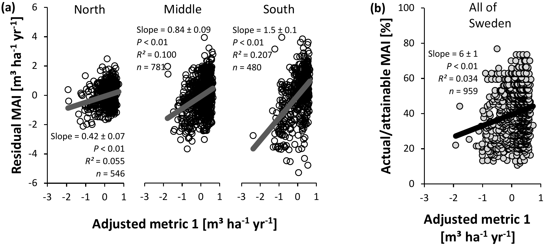
Figure 10Evaluation of adjusted nutrient availability metric 1 for Swedish conifer forests. (a) Method 1 – association with residual mean annual increments (MAIs) of the productivity–climate regression model (Fig. 3a, Eq. S1 and Table S2), distinguishing northern, middle, and southern Sweden. (b) Method 2 – association with actual ∕ attainable MAI (Fig. 3b) for the entire Swedish land area. Full line: significant slope (P < 0.05).

Download

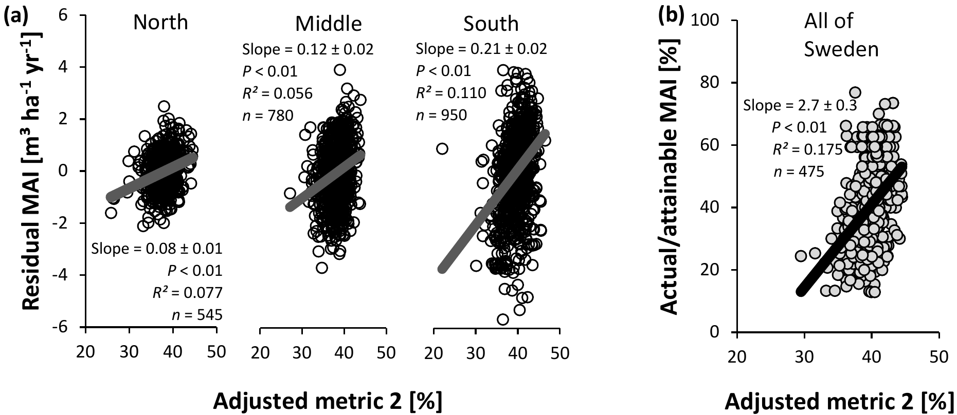
Figure 11Evaluation of adjusted nutrient availability metric 2 for Swedish conifer forests. (a) Method 1 – association with residual mean annual increments (MAIs) of the productivity–climate regression model (Fig. 3a, Eq. S1 and Table S2), distinguishing northern, middle, and southern Sweden. (b) Method 2 – association with actual ∕ attainable MAI (Fig. 3b) for the entire Swedish land area. Full line: significant slope (P < 0.05).

Download

Since soil moisture and soil type influenced both soil properties and normalized productivity, we also stratified the analyses above by these factors. In general, these separate analyses confirmed the robustness of the observed patterns across the database (despite low R²s), as the results and parameter estimates were similar to those of the previous analysis (Tables S5 and S6).

3.3 Question 2 – evaluation of the IIASA metric

Both methods agreed on the poor performance of the IIASA metric to elucidate patterns in nutrient availability, as the weakly positive correlation between normalized productivity and the metric was rarely significant, and explained < 1 % of the variation in normalized productivity in northern Sweden for method 1 (Fig. 9). Residual values of the relationship between normalized productivity of method 1 and the metric score (Fig. 9a) were significantly associated with all four input variables of the metric (SOC, soil texture, TEB, and pH_w – Table S9). SOC and TEB correlated negatively with these residuals, while sand was significantly positively related to these same residuals, and productivities at low pH_w were overestimated (the empirical quadratic functions were concave; not shown in Table S9). Residuals of method 2 (Fig. 9b) confirmed the negative trend with TEB but showed no statistically significant relationship with SOC, texture, or pH_w (Table S9). Overall, the fact that residuals were still correlated with the variables in the metric suggests that the input variables were not optimally implemented in the formula.

3.4 Question 3 – adjustments of the IIASA metric

From the statistical analyses for Question 1, we deduce that SOC, soil C : N, and pH each play a role in influencing nutrient availability in Sweden. Based on their relationships with normalized productivity in southern Sweden according to method 1 (Table S10), and in all of Sweden according to method 2 (Table S11), the following formulae were implemented in two adjusted nutrient availability metrics (Figs. S5 and S6):

for the metric based on method 1 (adjusted metric 1), and

for the metric based on method 2 (adjusted metric 2).

In the same way as for the IIASA metric, Eqs. (11)–(13) and (14)–(16) were combined in Eq. (10) to calculate the final nutrient availability score for each metric. Soil texture and exchangeable bases were not included here, as their empirical relationships with normalized productivity showed opposite trends compared to their implementation in the IIASA metric (Fig. 1 vs. Tables 2 and S9), likely due to indirect effects of soil moisture and related organic matter accumulation.

Table 4Evaluation of adjusted nutrient availability metric 1 for selected nutrient availability gradients in Sweden (Fig. S2). Statistics indicate the relationship between productivity (mean annual increment – m³ ha⁻¹ yr⁻¹) and the metric. For (near) significant variables (i.e., P<0.10), parameter estimates ± s.e.m. and the proportion of variation explained (R²) are given. For Norway spruce, no TEB gradient without substantial variation in climate was found, so that only for Scots pine was there a gradient in TEB. Abbreviations: TEB: total exchangeable bases. Error bars represent the s.e.m.

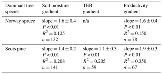
N/a: not applicable

Download Print Version | Download XLSX

In contrast to the IIASA metric of constraints on nutrient availability, the adjusted metrics were significantly related with normalized productivity (Figs. 10 and 11), albeit with low R² values. The same analyses stratified by soil moisture (Tables S12 and S14) gave similar results for the intermediate fresh and fresh-moist moisture classes (i.e., those with the majority of data points), while stratification by soil type generally weakened relationships between the metrics and normalized productivity (only for Podzols and Regosols, could the metrics always describe variation; Tables S13 and S15). Only on a few occasions did the soil variables included in metric 1 show a (borderline) significant correlation with the residuals of the relationship between normalized productivity and the adjusted metrics (and the associated R² values were always low (≤ 0.005); Table S16). We therefore conclude that SOC, soil C : N, and pH are generally well implemented in this adjusted metric, at least for the database considered here. For adjusted metric 2, however, significant associations with higher R² values emerged, thus indicating suboptimal implementation of the variables in the metric, but the sign of the significant slope differed depending on whether normalization method 1 or 2 was used (Table S17).

Five nutrient availability gradients were selected to evaluate the performance of the adjusted metrics in the absence of confounding climate and N deposition effects (Fig. S2). Both metrics were capable of describing variation in productivity for all gradients, with R² values of 0.092–0.383 (Tables 4 and 5). Variable implementation was generally good, except for SOC in adjusted metric 2. There, SOC was significantly negatively associated with the residuals of the productivity–metric relationship (for four out of five gradients; Tables S18 and S19). Both the results of the national database and the gradients thus indicate that the adjusted metrics explain part of the spatial variation in productivity, and that adjusted metric 1 performs better than adjusted metric 2. Further adjustments, for example with other soil variables, may be needed to increase their performance.

4.1 Identifying potentially confounding factors

Soil moisture varies between dry and very wet across Sweden and may obfuscate associations between nutrient-related soil properties and (normalized) productivity. Across our database, we indeed observed that certain soil properties (SOC, soil C : N ratio, TEB) were related with soil moisture (Fig. S3), and also normalized productivity depended on soil wetness (Fig. 5): productivity was highest for intermediate soil moisture levels, and was significantly reduced for the most dry and wet soils. The influence of soil moisture on productivity can be explained as follows: at high water content, the anoxic rooting environment inhibits root and microbial respiration. Tree productivity is thus suppressed, both directly due to the lack of oxygen for the tree itself and because nutrient supply is limited due to the inhibition of mineralization (Gorham, 1991). For relatively dry soils, however, productivity is reduced because of water limitation (which has been shown to occur in southern Sweden – Bergh et al., 1999), lower nutrient inputs through groundwater, fewer periods with easily available nutrients in the soil solution (Qian and Schoenau, 2002), and lower retention (Larcher, 2003; Roy et al., 2006) and supply (Binkley and Hart, 1989) of nutrients by organic matter. In summary, any associations between a soil variable and productivity should be interpreted in view of the fact that soil moisture may act as a factor influencing both this soil variable and productivity. We therefore performed our analyses not only for the complete set of data but also for the data stratified by soil moisture to assess whether relationships between soil properties and productivity would change.

In the same way as for soil moisture, stratification by soil type might help in resolving nutrient–productivity relationships. Soil properties and productivity differed among the five most common soil types in the database (i.e., Histosols, Gleysols, Regosols, Leptosols, and Podzols – Fig. S4). To some extent, these differences among soil types overlapped with those observed for soil moisture classes (e.g., wet Histosols had the highest SOC, soil C : N, and the lowest productivity), but additional patterns emerged as well (e.g., Podzols had a particularly low TEB stock). Although actual differences in nutrient availability among soil types will in part underlie the variations in productivity, other factors related to soil type (e.g., wetness, soil depth, or the rooting environment) may also influence productivity (Binkley and Hart, 1989). The main analyses of the current study were therefore stratified by both soil moisture and type to test the robustness of associations between nutrient-related soil properties and normalized productivity.

Many studies have shown the strong influence of N deposition on forest productivity (e.g., Laubhann et al., 2009; Solberg et al., 2009; de Vries et al., 2014; Binkley and Högberg, 2016; Wang et al., 2017). As expected, N deposition correlated to some extent with some of the soil variables considered in the present study, such as the total soil N stock and concentration (Fig. 4b). Furthermore, N deposition was strongly positively related to productivity. However, this effect of N deposition on productivity cannot be separated from the influence of climate and light, as all these factors increase together in the north–south direction. Nevertheless, we argue that for the goals of this study, i.e., investigating soil nutrient–productivity relationships across Sweden and developing a nutrient metric, the spatially varying N deposition is not problematic since the normalization for climate and species according to method 1 (Fig. 3a) at the same time also removed the influence of the confounding N deposition on productivity. Accordingly, residual productivity was generally not correlated with N deposition (Table S3). The response variable derived from method 2 (i.e., actual ∕ attainable productivities for spruce – Fig. 3b), in contrast, correlated strongly with N deposition (Table S4) because both actual ∕ attainable productivity and N deposition increased from north to south. Consequently, relationships between actual ∕ attainable productivity and soil data for this method were unavoidably confounded by N deposition.

Table 5Evaluation of adjusted nutrient availability metric 2 for selected nutrient availability gradients in Sweden (Fig. S2). Statistics indicate the relationship between productivity (mean annual increment – m³ ha⁻¹ yr⁻¹) and the metric. For (near) significant variables (i.e. P<0.10), parameter estimates ± s.e.m. and the proportion of variation explained (R²) are given. For Norway spruce, no TEB gradient without substantial variation in climate was found, so that only for Scots pine was there a gradient in TEB. Abbreviations: C : N: soil carbon-to-nitrogen ratio; TEB: total exchangeable bases. Error bars represent the s.e.m.

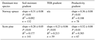
N/a: not applicable

Download Print Version | Download XLSX

4.2 Question 1 – normalized productivity vs. single and combined soil variables

Soil C : N ratio had a negative effect on normalized productivity for both methods (Figs. 7b and 8b). Apart from high N concentrations at low C : N, increased productivities with decreasing C : N ratio can follow from its influence on litter decomposition and mineralization, and thus on nutrient availability: when the ratio in organic matter is high, microbes more strongly immobilize N to adjust their internal C to N stoichiometry. As a consequence, N is not easily released and made available for plant uptake. A low C : N ratio, however, facilitates N mineralization (Roy et al., 2006) and thus enhances N availability (Wilkinson et al., 1999).

The relationship of ln SOC with normalized productivity, which showed an optimum (Figs. 7a and 8a), is partly explained by the role of SOM in storing and exchanging nutrients, but also partly by the confounding effect of soil moisture. At high moisture levels, SOC most likely increases because decomposition is reduced in water-saturated soils, leading to organic matter accumulation (Fig. S3a). Anoxic soils impede productivity because of the aforementioned prevention of root respiration and reduced supply of newly available nutrients through mineralization. At low SOC, however, productivity supposedly decreases with decreasing SOC because of water limitation and low availability of organic matter, which acts as a nutrient store. Together, these results suggest that the empirical relationship between SOC and productivity might have an optimum below which soil fertility is reduced due to a lack of sufficient organic matter, and above which high SOC indicates hostile rooting conditions and limited nutrient supply through slow mineralization. The first aspect is thus included in the IIASA metric (Fig. 1), while the decreasing part of the curve should be included in the empirical relationship of SOC with nutrient availability if the effect of reduced decomposition is not captured by any of the other soil variables in an updated metric.

Soil factors other than the soil C : N ratio and SOC either exhibited only a marginal influence on normalized productivity or their effect depended on the approach (Table 2). N stocks could explain variation across both methods, but their explanatory power was rather modest for method 1. We anticipate that if we aim to develop metrics applicable beyond the boreal biome, including N stock will be of limited value, as this variable is only loosely related to N availability (Högberg et al., 2017).

Mineral soil clay fractions had a weak but significantly positive effect on normalized productivity. Even though clay particles can protect SOM from decomposition (Xu et al., 2016), clay soils in the Swedish database in all likelihood positively influence nutrient availability by means of their negative charges that serve as cation exchange sites (i.e., for NH${}_{\mathrm{4}}^{+}$, K⁺, Ca²⁺, and Mg²⁺ – IIASA and FAO, 2012). Effects of TEB and pH were dependent on the method, possibly reflecting differences between regional (method 1) and national (method 2) variation in nutrient availability.

All equations resulting from multiple regression analysis combining different soil variables contained the soil C : N ratio and SOC (Table 3), confirming that, in the absence of direct soil nutrient data, these are key and complementary determinants of nutrient availability in northern coniferous forests. Qualitatively considered, associations of C : N ratio (−), SOC (concave quadratic after log transformation), N stock (+), and clay fraction (+) with normalized productivity were consistent for both approaches (Table 2). Together with their abilities to explain variation, the consistent effects of soil C : N and SOC suggest these soil variables have the most potential for inclusion in an improved nutrient availability metric.

4.3 Question 2 – evaluation of the IIASA metric

Although the IIASA metric of constraints of nutrient availability was originally designed for arable lands, we opted to start with this metric for a few reasons. Apart from the fact that to our knowledge it represents the only attempt so far to develop a generic nutrient metric, the structures of its formulas (Eqs. 6–9) reflect general mechanisms that link soil properties to nutrient availability, which are also valid for nonagricultural ecosystems. Soil pH for example shows a typical optimum effect on nutrient availability, while SOC and TEB have a direct positive nonlinear influence (IIASA and FAO, 2012). The final weighing of the four partial scores (Eq. 10) finds its rationale in the idea that if a certain soil property is particularly suboptimal, it will be the most important nutrient-related determinant of productivity, with less influence of the other soil properties that are closer to or within their optimal range. This way of weighing can be considered a type of interaction, but one that cannot be implemented in a simple linear regression model. Hence, our main reason for adopting the IIASA metric as a starting point is that, in spite of its simplicity, it is based on theoretical considerations. Moreover, adopting this structure allows for updating with other datasets – something that can probably not be achieved with multiple regression equations (see Sect. 4.4).

The IIASA metric of constraints on nutrient availability does not clarify much variation in normalized productivity among Swedish forests. Moreover, SOC, soil texture, TEB, and pH_w were apparently not optimally implemented. A low performance of the IIASA metric in its current form for the Swedish database was expected, as it was initially developed for evaluating (constraints on) the soil fertility of agricultural ecosystems, and the Swedish database contains variable values outside the ranges to which the metric is sensitive. Soil conditions of agroecosystems indeed greatly differ from the boreal forests investigated in the present study. Many Swedish forest soils are for instance coarse textured, and in addition, the database contains wet-soil forests, while arable soils are typically not water saturated.

4.4 Question 3 – adjustments of the IIASA metric

Based on results of the analyses for Question 1, the nutrient availability metric was adjusted by (i) including an empirical optimum in the influence of SOC on normalized productivity, and (ii) including soil C : N, thus more explicitly incorporating the availability of N. In the current analysis, soil texture and TEB were excluded from the metrics, as they exhibited negative instead of the expected positive associations with normalized productivities (IIASA and FAO, 2012), probably due to indirect effects of low soil oxygen, reduced decomposition, and suppressed productivity where the proportion of sand is low and TEB is high.

In contrast to the original metric developed by IIASA, the adjusted metrics described some variation across all approaches using the full database (Figs. 10 and 11). Variables were generally properly implemented, at least for the adjusted metric 1 (Table S16). For metric 2, significant (but normalization-method-dependent) associations emerged between residuals of normalized productivity and SOC and pH (Table S17). The stratified analyses confirm that the metrics are an improvement, at least for those soil moisture classes and soil types with sufficient data points (Tables S12–15). Moreover, each metric could describe spatial variation in productivity for five manually selected local nutrient availability gradients (Tables 4 and 5). The coefficients of determination were generally higher for these gradients than for the database analyses, likely because the gradients did not require a normalization for climate (the latter increased the uncertainty on the response variable; see Sect. 4.5 on sources of uncertainty and future challenges). Lastly, the gradients generally confirmed the correct implementation of soil variables in adjusted metric 1 (Table S18), whereas for metric 2, scores for high SOC might be overestimated (Table S19).

Variation in normalized productivity explained by the adjusted metrics (R² = 0.03–0.21 and R² = 0.06–0.18) was similar to the variation explained by multiple regression equations (R² = 0.18–0.22) that contained the same (and more) soil variables as the metrics. The metrics, however, have the advantage that they can be updated more easily than equations from multiple regressions, especially if additional soil parameters need to be included for other ecosystems. Moreover, the interaction effect – with the highest weight for the least optimal soil parameter – cannot be mimicked with a multiple regression approach. In order to further adjust the metrics, and to test to what extent they can already describe variation in nutrient availability outside of Swedish conifer forests, additional datasets with productivity and soil information are needed. Such datasets include large-scale inventories such as the one considered in the present study, but also local gradients and nutrient manipulation experiments. The latter two have lower generalizability, but offer the advantage that normalization for climate is not needed.

4.5 Sources of uncertainty and future challenges

Even though normalized productivity was significantly related to soil properties, and to our adjusted metrics, much of the variation in normalized productivity remains unexplained. The considerable unexplained variation may have multiple reasons. Apart from a possible lack of soil and nutrient data more closely related to N availability than the ones available in our database, another possible factor reducing R² values could be the quality of the data in the database. This could for instance be due to an insufficient number of replicates sampled per data point (n= 3 for the soils), although this is probably of limited importance because of the large number of data points in the database itself. A more important source of uncertainty is probably the inevitable uncertainty related to the response variable, i.e., climate-normalized aboveground productivity. This includes uncertainty in the original productivity estimates (for example, for which differences in management or disturbances likely increased variability) and additional variation caused by soil moisture effects on oxygen availability (which we accounted for by also performing analyses on split datasets). However, there is also uncertainty related to the normalization for climate: by taking residuals of the productivity vs. climate regression model (method 1), we for instance unintentionally removed not only the direct effect of climate on productivity but also its indirect effect through nutrient availability. Normalized productivity based on this method thus mainly represents productivity as influenced by regional variation in nutrient availability. The approach taking actual ∕ attainable productivity as a response variable (method 2) does not suffer from this issue, but there the estimates of attainable productivity come with a high uncertainty, as they were based on only limited experimental data to establish a relationship between productivity and intercepted radiation. As a consequence, the low R² values are partly due to shortcomings of the normalization procedure that can only be overcome by using datasets in which climate does not vary but nutrient availability does. Such datasets are provided by local gradients, such as the five local nutrient availability gradients that we selected from our database for additional evaluation of our adjusted metrics.

The similar and significant results for the different methods (1 and 2) and subsets of the database (regions, soil moisture classes, and soil types) indicate that the findings about the soil properties and nutrients are generally robust. The adjusted metrics explained up to 21 % of the variation in normalized productivity. It is unclear to what degree the influence of nutrient availability is covered by this percentage. Future studies, in which additional soil data (e.g., P) can be included, will need to verify this. In any case, the significant relationships with normalized productivity, the better implementation of the soil variables, and the capability of the metrics to explain up to 38 % of the variation in productivity across different gradients imply a significant improvement compared to the original IIASA metric for this database.

A key challenge in the further development of a metric describing spatial variation in nutrient availability both within and outside the boreal biome is differential nutrient limitation. Eventually, we want to be able to compare for example N-limited and P-limited systems. The original structure of the IIASA metric, which was kept in our adjusted metrics, facilitates this by allowing the inclusion of multiple soil variables such as soil C : N (mainly relating to N availability), pH (among others a critical factor controlling P availability), and TEB in one single metric. In fact, the IIASA metric is particularly useful in this regard, as it gives more weight to the soil factor with the lowest score. This corresponds to reality and enables accounting for the type of nutrient limitation. For instance, if soil C : N is high, indicating N limitation, the metric score will be substantially reduced by this high C : N, while at low C : N other limiting factors can dominate the metric score.