the Creative Commons Attribution 4.0 License.
the Creative Commons Attribution 4.0 License.
 | 18 May 2018
Groundwater data improve modelling of headwater stream CO2 outgassing with a stable DIC isotope approach
Marcus Conrad
Vadym Aizinger
Alexander Prechtel
Robert van Geldern
Johannes A. C. Barth
A large portion of terrestrially derived carbon outgasses as carbon dioxide (CO2) from streams and rivers to the atmosphere. Particularly, the amount of CO2 outgassing from small headwater streams is highly uncertain. Conservative estimates suggest that they contribute 36 % (i.e. 0.93 petagrams (Pg) C yr−1) of total CO2 outgassing from all fluvial ecosystems on the globe. In this study, stream pCO2, dissolved inorganic carbon (DIC), and δ13CDIC data were used to determine CO2 outgassing from an acidic headwater stream in the Uhlířská catchment (Czech Republic). This stream drains a catchment with silicate bedrock. The applied stable isotope model is based on the principle that the 13C ∕ 12C ratio of its sources and the intensity of CO2 outgassing control the isotope ratio of DIC in stream water. It avoids the use of the gas transfer velocity parameter (k), which is highly variable and mostly difficult to constrain. Model results indicate that CO2 outgassing contributed more than 80 % to the annual stream inorganic carbon loss in the Uhlířská catchment. This translated to a CO2 outgassing rate from the stream of 34.9 kg C m−2 yr−1 when normalised to the stream surface area. Large temporal variations with maximum values shortly before spring snowmelt and in summer emphasise the need for investigations at higher temporal resolution. We improved the model uncertainty by incorporating groundwater data to better constrain the isotope compositions of initial DIC. Due to the large global abundance of acidic, humic-rich headwaters, we underline the importance of this integral approach for global applications.
- Article
(2715 KB) -
Supplement
(381 KB) - BibTeX
- EndNote


Rivers and streams are the main carbon pathways from the continents to the oceans and thus constitute an important link in the global carbon cycle. In the process of transport, large amounts of carbon – mostly in the form of CO2 – outgas from the water surface to the atmosphere (Cole et al., 2007; Aufdenkampe et al., 2011; Regnier et al., 2013; Wehrli, 2013). Globally, this form of CO2 contributions to the atmosphere was estimated between 0.6 and 2.6 petagrams (Pg) of carbon per year (Raymond et al., 2013; Lauerwald et al., 2015; Sawakuchi et al., 2017; Marx et al., 2017a). The lower value of this range by Lauerwald et al. (2015) excluded streams of Strahler stream numbers below 3. This is because of sparse coverage of actual direct measurements of the partial pressure of CO2 (pCO2) in headwater streams. Note that the upper value of the range still lacks a representative contribution from headwater streams (Marx et al., 2017a).
The contributions of headwater streams are considered as a major unknown factor in these estimates of global carbon budgets for inland waters (Cole et al., 2007; Raymond et al., 2013). The main reasons are uncertainties in groundwater input as well as poorly defined surface areas and gas transfer velocities (Marx et al., 2017a; Schelker et al., 2016). In addition, pCO2 and subsequent CO2 outgassing fluxes typically decline rapidly from stream source areas to river sections further downstream (van Geldern et al., 2015; Stets et al., 2017). Poor definition of these gradients adds another uncertainty to the global carbon budget. The enormous number of small headwater streams making a significant contribution on a basin and thus on the continental scale combined with the scarcity of data led to the term aqua incognita (Bishop et al., 2008).
Various direct and indirect approaches to determine CO2 fluxes exist. Most often fluxes are calculated from pCO2 and gas transfer velocities (Teodoru et al., 2009; Raymond et al., 2012; Lauerwald et al., 2015; van Geldern et al., 2015). However, because of large variabilities of gas transfer velocities on different spatial and temporal scales, this type of determination remains controversial, especially for small-scale applications (Marx et al., 2017a; Regnier et al., 2013; Schelker et al., 2016). For applications in small streams and during changing flow conditions, direct methods such as floating chamber approaches also exhibit major drawbacks such as altered outgassing behaviour because of artificially created currents inside anchored chambers (Lorke et al., 2015; Bastviken et al., 2015). In addition, rapid downstream losses of CO2 often imply that CO2-rich groundwater inputs are lost before actual measurements can take place (Reichert et al., 2009).
Recent approaches have used stable carbon isotopes of dissolved inorganic carbon to reliably quantify CO2 outgassing from streams and rivers (Polsenaere and Abril, 2012; Venkiteswaran et al., 2014), in which the model by Venkiteswaran et al. (2014) is a parsimonious, simpler version of the model by Polsenaere and Abril (2012). Both apply inverse modelling to calculate the amount of CO2 lost upstream of a sampling point within a stream or at a catchment outlet. One clear advantage when compared to conventional methods is that these stable isotope approaches account for the potentially high CO2 outgassing upstream of any sampling point. Moreover, they incorporate groundwater seeps in first-order headwaters, particularly at low discharge (Polsenaere and Abril, 2012). These factors are typically not covered by conventional methods.
The integrative models exploit the fact that stable isotope ratios of dissolved inorganic carbon (expressed as δ13CDIC) in stream water are controlled by 13C ∕ 12C ratios of its sources and the intensity of CO2 outgassing. One important input is the stable isotope ratio of soil CO2, which in turn depends on the plants' pathways used for photosynthesis and the organic matter sources fuelling plant and microbial respiration (Mook et al., 1983; Vogel, 1993). In general, this soil-internally produced CO2 has a value close to the initial substrate, which has a range from −30 to −24 ‰ for the most commonly occurring C3 plants (Ehleringer and Cerling, 2002). After entering the stream, CO2 outgassing to the atmosphere increases 13C ∕ 12C ratios in the remaining DIC pool because of the well-known equilibrium isotopic fractionation between CO2, , and (Myrttinen et al., 2015, 2012; Mook et al., 1974). This predictable and temperature-related process is calculated by the models of Polsenaere and Abril (2012) and Venkiteswaran et al. (2014). They are independent of the gas transfer velocity k and account for the upstream portion of a sampling site in headwater streams.
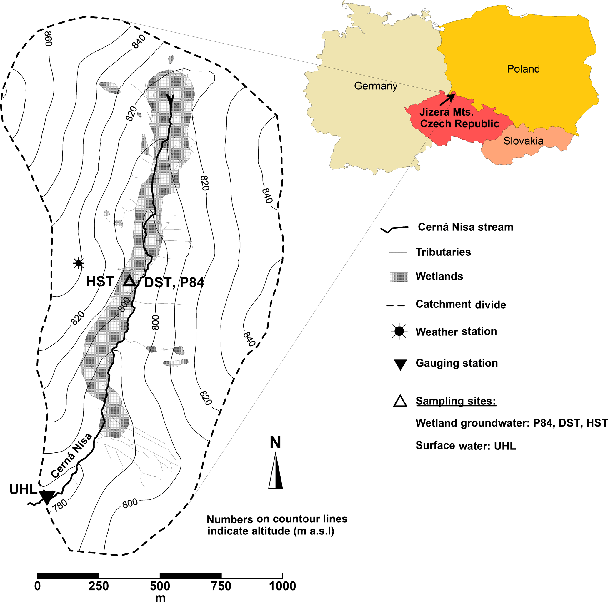
Figure 1Location of the Uhlířská catchment and sampling sites modified from Sanda et al. (2014).
The aim of this work was to model stream CO2 outgassing on the basis of the stable isotope approach by Polsenaere and Abril (2012) and to extend their method by including measured groundwater stable isotope composition in order to reduce modelling uncertainties. Our study utilises data from the well-studied Uhlířská catchment in the Jizera Mountains (Czech Republic) (Dusek et al., 2012; Sanda et al., 2014; Vitvar et al., 2016; Marx et al., 2017b). Since the background geology of the catchment consists of silicate rocks, carbonate weathering as a CO2 source can be virtually excluded. The CO2 saturation is then exclusively controlled by the mobilisation of terrestrial respired organic carbon and by the input of shallow groundwater (Humborg et al., 2010; Amiotte-Suchet et al., 1999).
2.1 Study site
The Uhlířská catchment is situated in the northern Czech Republic, 9 km northeast of the city of Liberec (Fig. 1). The stream Černá Nisa flows in the catchment valley and is a tributary of the Lužická Nisa River that later merges with the Odra River and flows towards the Baltic Sea. The stream length in this experimental catchment is about 2100 m and water travel times are less than 1 h from the spring to the catchment outlet.
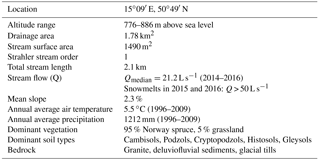
Table 1 lists the main characteristics of the Uhlířská catchment. The annual average precipitation exceeds 1200 mm yr−1 and the annual average temperature is 5.5 ∘C (1996–2009). Snow cover typically prevails during 6 months of the year, mostly between November and March (Hrncir et al., 2010). During our study period from September 2014 to April 2016 snow cover prevailed only between January and March. However, during snowmelt the monthly average discharge doubles (> 50 L s−1) compared to the other months' discharges (Table 1).
The forest consists of a spruce monoculture (Picea abies) and isolated patches of larch, beech, and rowan trees (Sanda and Cislerova, 2009). Purely granitic bedrocks underlie this type of C3 vegetation. The catchment has two basic types of soils. On the hillslopes, about 60–90 cm deep and highly heterogeneous soil profiles consist of dystric Cambisols, Podzols or Cryptopodzols that developed on weathered and fractured bedrocks. These soil types cover approximately 90 % of the catchment area. The valley bottom soils consist of a layer of peat of mostly Histosol types with depths up to 300 cm. The latter soils cover approximately 10 % of the catchment area, make up small wetlands along the stream and lie on top of fluvial material, which embodies the main perennial aquifer (Sanda et al., 2014).
Table 1Characteristics of the Uhlířská catchment and Černá Nisa stream.
2.2 Water sampling and laboratory analyses
Between September 2014 and April 2016 shallow wetland groundwater and stream water were collected on a monthly basis and approximately weekly basis, respectively. Sampling points are shown in Fig. 1.
The stream discharge was determined at a V-notch weir at the catchment outlet (site UHL; see Fig. 1). Temperature (T), pH, and total alkalinity (TA) were determined in the field with portable HACH equipment, including a multi-parameter instrument and a digital titrator (all HACH Company, Loveland, CO, USA). The measured parameters exhibited a precision of 0.1 pH units, 0.1 ∘C (2σ) for T and was better than 2 % (2σ) per 100 titration steps for TA (Marx et al., 2017b). Water samples were collected from the stream approximately 10 cm below the water surface and from boreholes with a peristaltic pump approximately 24 h after purging the boreholes.
Particulate organic carbon (POC) was sampled on 0.7 µm pore size glass fibre filter papers and analysed according to Barth et al. (2017). All other samples were filtered via syringe disk filters with 0.45 µm pore size (Minisart HighFlow PES, Sartorius AG, Germany) in the field. Before filtration, both syringe and membrane were pre-washed with sample water. Samples for the analysis of dissolved inorganic carbon (DIC) concentrations and isotopes were collected in 40 mL amber glass vials without headspace. The vials fulfil specifications of the US Environmental Protection Agency (EPA) and were closed with butyl rubber/PTFE septa and open-hole caps, with butyl rubber side showing towards the sample. Vials were poisoned with 20 µL of a saturated HgCl2 solution to avoid biological activity after sampling. After collection, all samples were kept in the dark at 4 ∘C until analyses.
Water samples were analysed for their carbon stable isotope ratio of dissolved inorganic carbon (δ13CDIC) by an OI Analytical Aurora 1030W TIC-TOC analyser (OI Analytical, College Station, Texas) that was coupled in continuous flow mode to a Thermo Scientific Delta V plus isotope ratio mass spectrometer (IRMS) (Thermo Fisher Scientific, Bremen, Germany). The sample was reacted with 1 mL of 5 % phosphoric acid (H3PO4) at 70 ∘C for 2 min to release the dissolved inorganic carbon (DIC) as CO2. The evolved CO2 was purged from the sample by helium. The Aurora 1030W system uses organic materials (see below) for the calibration to the VPDB scale and for concentration measurements. To oxidise these materials to CO2, 2 mL of 10 % sodium persulfate (Na2S2O8) was reacted for 5 min at 98 ∘C. A trap and purge (T&P) system was installed for the analysis of low concentrations. Details of the coupling of the TIC/TOC analyser to IRMS are described in St-Jean (2003).
All values are reported in the standard δ notation in per mil (‰) vs. Vienna Pee Dee Belemnite (VPDB) according to
where R is the ratio of the numbers (n) of the heavy and light isotope of an element (e.g. n(13C) ∕ n(12C)) in the sample and the reference (Coplen, 2011). The data sets were corrected for instrumental drift during the run and linearity. Then they were normalised to the VPDB scale by two laboratory reference materials (C4 sugar and KHP) measured in each run. The in-house reference materials were calibrated directly against USGS-40 (L-glutamic acid) and IAEA-CH-6 (sucrose) by using an elemental analyser (Costech ECS 4010). A value of −26.39 and −10.45 ‰ was assigned to USGS-40 and IAEA-CH-6, respectively. Concentration was determined from the signal of the OI Aurora 1030W internal non-dispersive infrared sensor (NDIR) and a set of calibration standard with known concentrations prepared from analytical (A.C.S.)-grade potassium hydrogen phthalate (KHP). Analytical precision based on the repeated analyses of a control standard (C3 sugar) during all runs was better than ±0.3 ‰ for δ13C and better than 5 % for concentrations (1σ).
POC samples were analysed for δ13CPOC using a Costech Elemental Analyser (ECS 4010; Costech International, Pioltello, Italy; now NC Technologies, Bussero, Italy) coupled in continuous flow mode to a Thermo Scientific Delta V plus IRMS. The data sets were corrected for linearity and instrumental drift during the run. Values were normalised for carbon to the VPDB scale by analyses of internal reference materials (C4 sugar and KHP) that were calibrated directly versus USGS-40 and USGS-41 (L-glutamic acid). Assigned values to USGS-40 and USGS-41 were −26.39 and +37.63 ‰ for δ13C, respectively. For precision and accuracy two laboratory standards (acetanilide and tartaric acid) were measured in each run. Precision, defined as the standard deviation of the control standard, was better than 0.1 ‰ (1σ) for δ13CPOC.
2.3 Calculations and model assumptions
At the Uhlířská headwater catchment the original streamCO2-DEGAS model was applied to calculate stream CO2 outgassing for different scenarios with varying values of river respiration (R) with 10, 19, 25, 50, and 75 % to test the model sensitivity to these values. In a second approach we modified the streamCO2-DEGAS model as follows: instead of soil organic matter (δ13CSOM) we used groundwater δ13CDIC data to better constrain initial CO2 values and to reduce the model uncertainty.
The Uhlířská catchment meets the assumption of the streamCO2-DEGAS model with (i) stream waters being acidic with pH values between 3.9 and 6.7 (Table 2), and for our study we assumed that (ii) waters in the stream are unproductive. This means that secondary processes such as photosynthesis by algae or biofilms and organic matter (OM) degradation to CO2 are neglected. This is a plausible assumption because high runoff and short residence times often leave insufficient time for substantial degradation of OM (Raymond et al., 2016; Catalan et al., 2016). However, the potential of temperature-dependent in-stream bio- and photodegradation (Demars et al., 2011; Moran and Zepp, 1997), particularly during summer, cannot be entirely excluded in the Černá Nisa stream.
The original streamCO2-DEGAS model by Polsenaere and Abril (2012) demands the input variables of total alkalinity (TA), δ13CDIC, pCO2, and temperature (Table 2), as well as the proportion of river respiration (R) and the carbon isotope composition of δ13CSOM. Note that TA and groundwater δ13CDIC were only measured during monthly samplings and linear interpolated otherwise.
We used DIC concentrations to calculate (Dickson, 2007), and together with pH and T we were able to calculate pCO2 values with the following equation (Plummer and Busenberg, 1982):
where is the activity of bicarbonate, H+ is 10−pH, K1 is the temperature-dependent first dissociation constant for the dissociation of H2CO3 (all variables in mol L−1), and KH is the Henry's law constant in mol L−1 atm−1. The uncertainty of the calculation depends on the measurement uncertainties of DIC, pH, and T. The largest uncertainty is caused by pH measurements as they are on a logarithmic scale. The pH measurement uncertainty is typically smaller than ±0.1 pH units and causes a maximum uncertainty of ±21 % for pCO2. We consider this a worst-case scenario, which is also indicated in Fig. 3.
R (0<R<1) is the proportion of CO2 resulting from respiration in water along the entire stream course (waterlogged soils, stream waters, and sediments) and was approximated by a range between 0.1 and 0.19 (i.e. 10 to 19 %). This corresponds to the credible range of internal CO2 production as a percentage of median stream CO2 emissions from small streams (< 0.01 m3 s−1) in the contiguous United States and was determined by Hotchkiss et al. (2015).
According to Polsenaere and Abril (2012) POC was used as representative of catchment soil organic matter. Polsenaere and Abril (2012) chose a δ13CSOM of −28 ‰ that was determined as average annual δ13CPOC at their study site. In our study we also used the average annual stream δ13CPOC. Thus the δ13CSOM was confined with −29.5 ‰ (Table 2). In addition, the average of wetland groundwater δ13CDIC with an assumed isotopic fractionation of +1 ‰ for movement of CO2 in waterlogged soils, groundwaters, river waters and sediments (O'Leary, 1984), served as input of initial δ13CDIC (δ13C-DICinit). Measured δ13CDIC values ranged between −25.2 and −10.1 ‰ (Supplement).
The model results are the partial pressure of initial CO2 before gas exchanges (pCO2init) with the atmosphere start and the fraction of stream DIC that has degassed into the atmosphere ([DIC]ex). [DIC]ex corresponds to the CO2 loss upstream of the sampling point and is given as a concentration (Polsenaere and Abril, 2012). CO2 fluxes were calculated by multiplication with average discharges that were established from daily values. To allow for inter-catchment comparisons the carbon losses were normalised to the stream surface area. In addition, to avoid often imprecise stream lengths and surface areas, the carbon losses were also normalised to the catchment area.
For comparison, the gas transfer velocity adjusted to the in situ temperature (kT, in m d−1) can be calculated from model results when assuming that the water (pCO2,aq) is the average between the modelled soil pCO2 and the in situ pCO2 at the catchment outlet:
where F is the modelled CO2 outgassing (in g m−2 d−1), pCO2,air the partial pressure of CO2 in the atmosphere considered with ∼ 400 ppmV (ESRL/GMD, 2017), KH is the Henry's law constant (in mol L−1 atm−1) and MC the molar mass of C (12.011 g mol−1). kT was then converted into the normalised gas transfer velocity of CO2 at 20 ∘C (k600, in m d−1) according to
where ScT is the Schmidt number at the measured in situ temperature (Raymond et al., 2012).
All modelling approaches were executed via MATLAB (MathWorks, Natick, MA, USA).
2.4 Model input variables from the Uhlířská catchment
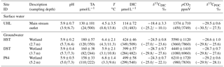
Stream (UHL) and wetland groundwater (DST, HST, P84) pH values were always below 6.7 during the entire study period (Table 2). In agreement with generally low stream pH values, the capacity of waters to buffer acidic inputs indicated by TA was generally low. The TA ranged around a median of 130 µmol L−1 with a standard deviation (1σ) of ±101 µmol L−1 at the catchment outlet (Table 2). Note that in the following the standard deviations express the variation over the sampling period and not the measurement error. The δ13CDIC values had a median of −18.4 ‰ with a range from −25.2 to −10.1 ‰ (Table 2). The most negative values were measured in wetland groundwater with median values of −24.5, −28.7 and −24.3 ‰ in HST, DST, and P84, respectively (Fig. 1). The range of these groundwaters between −23.6 and −29.6 ‰ fits the range of δ13C in C3 plants and associated soil organic matter. In the different water compartments (wetland groundwater and stream, Table 2), the DIC concentrations decreased with increasing δ13CDIC values. The lowest DIC concentrations were found at the catchment outlet (31 to 483 µmol L−1) and the highest concentrations in wetland groundwater (284 to 540 µmol L−1). The median stream pCO2 determined at the catchment outlet was 1374 ±710 ppmV with a range from 450 to 3749 ppmV. Values in wetland groundwater were typically higher with median values of 5590, 4440, and 6210 ppmV at HST, DST, and P84, respectively. Stream water temperatures showed a characteristic annual trend with a range from 0.8 to 13.8 ∘C and a median of 4.5 ∘C (Table 2).
Table 2pH, total alkalinity (TA), temperature (T), pCO2 values, DIC concentrations and 13C ∕ 12C ratios expressed as median values with ±1σ standard deviation and ranges given in parentheses. Site names are according to Fig. 1.
Our study shows that the uncertainty of the respiration parameter (R) can be circumvented by incorporating wetland groundwater δ13CDIC into the streamCO2-DEGAS model. In a first step the original CO2-DEGAS model was run with an R value of 10, 19, 25, 50, and 75 %. In a second step fractionation-corrected groundwater δ13CDIC was incorporated into the model. Thus the isotope composition of the initial CO2 was better constrained and the uncertainty on the isotope fractionation in soils was reduced.
In addition, we were able to estimate DIC export with modelled CO2 outgassing and calculated lateral export of , CO, and total DIC (Table 3). These data cover a period of 20 months and measurements took place at the catchment outlet, whereas modelling results relate to CO2 outgassing between the stream source and the catchment outlet (UHL). The Supplement for this article contains detailed analytical data used for model calculations in this study. It is accessible through the journal's website and is additionally archived in the World Data Center PANGAEA (https://doi.org/10.1594/PANGAEA.889689) for long-term storage and free access.
3.1 Model sensitivity
The parameter of proportion river respiration (R) has a large impact on the results by the model. It is attributed to the average percentage of respiration occurring along the entire stream course (waterlogged riparian soils, stream waters, sediments, and the hyporheic zone). Thus, it is important to evaluate the model sensitivity to the assumed respiration. Modelled CO2 outgassing and modelled initial pCO2 values relate to an assumed R of 10 and 19 %, which corresponds to an average in-stream respiration as determined by Hotchkiss et al. (2015). However, this value does not account for respiration in groundwater and soil water. The contributions of these compartments are typically also considerable in headwaters. Although this type of respiration was not measured directly, we can assume a large potential of respiration in waters of the organic-rich wetland and of riparian soils with peak values during late summer and early autumn (Pacific et al., 2008). In addition, respiration in gravel bar waters along the stream (Boodoo et al., 2017) can lead to an exceedance of 19 % for R along the Černá Nisa stream.

Figure 2Data of measured discharge, in situ pCO2, δ13CDIC, DIC concentrations, and CO2 fluxes calculated via model equations in Raymond et al. (2012) for the Uhlířská catchment outlet (UHL) (a) and modelled soil pCO2 and CO2 loss, as well as k600 calculated from model results and CO2 outgassing normalised to the stream surface area (b).
In some cases the model was not able to produce reliable results and the convergence criteria were not fulfilled. The initial soil pCO2 had to be extremely large (> 150 000 ppmV) for selected sampling events to reach the convergence of both δ13CDIC and pCO2 at the same iteration (Polsenaere and Abril, 2012). This was during few cases in February and March 2015 and during summer between May and September 2015. Moreover, for an R of 10 to 19 % during 22 to 23 cases, for an R of 25 and 50 % during 26 cases, and for an R of 75 % during 29 cases, the convergence criteria were not attained. Consequently, with increasing R a necessary convergence was more often not possible due to exceeding reasonable boundaries. These findings suggest that 10 to 19 % are reasonable R values for most months, except for June to August in 2015. Low respiration values are plausible for springtime; however, during summer an increased respiration can be assumed due to warmer temperatures and increased biological activity. One possible explanation for higher model uncertainty during summer is that the modelled CO2 loss shows a strong non-linear dependence on in situ pCO2 and δ13CDIC (Polsenaere and Abril, 2012). Thus, the relative error of modelled CO2 loss increases with the modelled CO2 loss itself. This is particularly the case for low TA (e.g. 0.1 mmol L−1; Polsenaere and Abril, 2012), where the δ13CDIC increase is not buffered by the pool. According to Polsenaere and Abril (2012), large losses of CO2 only occur with high in situ pCO2 and with high δ13CDIC. TA was low with 218 and 196 µmol L−1 in the Uhlířská catchment during June and July 2015. In contrast, δ13CDIC values and in situ pCO2 were increased with on average −15.8 and −16.2 ‰ as well as 2225 and 2411 ppmV, respectively. Thus, increased δ13CDIC values together with the model's non-linear dependence on in situ pCO2 and δ13CDIC may have caused an overestimation of modelled CO2 losses and – as a consequence – led to failed convergence criteria during summer. Note that processes such as photosynthesis, which are not part of the model, may also lead to increased δ13CDIC and lower in situ pCO2 values. This may further increase the uncertainty of model results.
3.2 Gas transfer velocities
A huge benefit of the applied isotope approach is that the difficult to estimate gas transfer velocity parameter (k) is not needed for the calculation of CO2 outgassing fluxes. On the other hand, k600 (gas transfer velocity of CO2 at 20 ∘C, Eq. 4) values could be estimated from model results when assuming the water pCO2 being the average between the modelled soil pCO2 and the in situ pCO2 at the catchment outlet (Table 3; Fig. 2).
For the original model calculated k600 values varied from 0.5 to 7.0 and from 0.6 to 7.9 m d−1 for R= 10 and 19 % (Table 3), with higher values mostly occurring during springtime and lower values during summer (Fig. 2). These values were higher than k600 values that were determined in a lowland boreal landscape of Québec (Campeau et al., 2014) (Table 4). However, values were slightly higher than in the silicate Renet catchment in France (1.2–7.2 m d−1) and were comparable to results from temperate silicate catchments in Germany (Halbedel and Koschorreck, 2013) (Table 4). They also equalled median values for boreal and Arctic streams (latitude 50–90∘) determined by Aufdenkampe et al. (2011), whereas k600 values for Sweden, for the United States, and for this study – all determined with model equations (i.e. Raymond et al., 2012) – showed higher values (Table 4). For modelling with groundwater data, we obtained lower k600 values than with the original model (Table 3). Values ranged from 0.1 to 5.4 m d−1 (Table 3) with higher values during springtime and lower values during summer (Fig. 2). The mean k600 value was similar to the value of 2.2 m d−1 calculated from gas transfer coefficients for propane in the temperate Zillierbach stream in Germany (Table 4).
Table 3DIC partitioning according to the streamCO2-DEGAS model (Polsenaere and Abril, 2012) and calculated from DIC measurements from September 2014 to April 2016 in the Uhlířská catchment expressed as median/average values ±1σ standard deviation and ranges given in parentheses. The total DIC export corresponds to the sum of export, CO export, and CO2 outgassing. Initial soil pCO2 was calculated from DICinit., pH and temperature. k600 was calculated from model results.
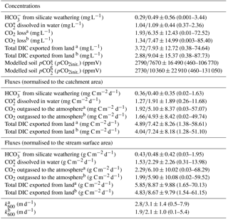
a Modelling with proportion river respiration (R)=10 and 19 %. b Modelling with groundwater data.
Table 4Gas transfer velocities (k600) normalised to a stream temperature of 20 ∘C of low order streams. Values calculated from model results are displayed in Table 3.
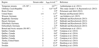
a Mean values. b Median values. c Running waters in Aufdenkampe et al. (2011) have < 60–100 m width.
3.3 Soil pCO2
The streamCO2-DEGAS model assumes that the modelled initial pCO2 represents soil pCO2 (Polsenaere and Abril, 2012). For the Uhlířská catchment, this would mean that soil pCO2 values ranged between 460 and 106 770 ppmV for original model and between 460 and 131 050 ppmV for modelling with groundwater input (Table 3). These were mostly within the range of values reported by Amundson and Davidson (1990), who determined pCO2 from 400 to 130 000 ppmV for the upper metre of soils around the world. For three acidic catchments in France, modelled soil pCO2 varied between 2120 and 77 860 ppmV (Polsenaere and Abril, 2012). In a temperate hardwood-forested catchment Jones and Mulholland (1998) modelled soil pCO2 values between 907 in winter and 35 313 ppmV in summer. Higher soil pCO2 values were also modelled during summer in the Uhlířská catchment. The main reasons for elevated soil pCO2 in warmer seasons are higher temperatures with enhanced soil respiration in summer (Jones and Mulholland, 1998).
A clear positive correlation between soil pCO2 and CO2 outgassing for modelling with groundwater inputs (r2 > 0.96, Supplement) stresses the importance of soil pCO2 values and their dynamics for stream CO2 loss.
3.4 CO2 outgassing
Figure 3a displays modelled CO2 outgassing for the proportion of river respiration (R) inputs that were selected with 10, 19, 25, 50, and 75 %. Figure 3b displays results for the modified modelling with groundwater input. Shaded areas show pCO2 measurement uncertainties. Points that plot outside the measurement uncertainty did not fulfil the convergence criteria (Polsenaere and Abril, 2012). They were thus replaced by interpolated values. Note that, for modelling with groundwater, data the fluxes where the convergence criteria were not fulfilled could become reduced by ∼ 50 % (Fig. 3b).
For modelling with R=10 % and 19 % the modelled CO2 outgassing varied from 0.01 to 72.52 mg C L−1 and showed a mean of 6.35 mg C L−1 (Table 3). When normalised to the catchment area, fluxes showed a mean of 5.10 mg C m−2 d−1 with values from 0.03 to 57.07 mg C m−2 d−1.
The highest fluxes > 30 mg C m−2 d−1 were modelled in May 2015, September 2015, November 2015, and March 2016 (Fig. 2). Translating these results to annual carbon outgassing fluxes yielded a mean of 23.9 to 34.5 g C m−2 yr−1 for 12 consecutive months and R= 10 and 19 %. Normalised to the stream surface area, an average of 28.6 to 41.3 kg C m−2 yr−1 was outgassed annually.
When including shallow wetland groundwater data in the model, the mean CO2 outgassing was 1.34 mg C L−1 and varied from 0.003 to 85.40 mg C L−1, with minimum and maximum values during April 2016 and June 2015 (Table 3). Corresponding fluxes with a mean of 8.8 kg C d−1 and a maximum of 88.5 kg C d−1 were smaller when compared to mean CO2 losses of 952, 258, and 10 671 kg C d−1 for similar organic-rich catchments in France calculated with the same model approach (Polsenaere and Abril, 2012). However, stream discharge in the French catchments was larger by at least 1 order of magnitude, thus yielding higher outgassing rates. When normalised to the catchment area, modelled CO2 losses had a mean of 4.9 mg C m−2 d−1 and varied from 0.02 to 49.7 mg C m−2 d−1 in the Uhlířská catchment. These values translate to a mean of 5.9 g C m−2 d−1 and a range between 0.02 and 59.5 g C m−2 d−1 when normalised to the stream surface area. Those groundwater-improved CO2 outgassing estimates yielded the same outgassing trend with slightly decreased values (Fig. 3).
The most used method to calculated CO2 fluxes is via k values, which are predicted via slope, flow velocity, stream depth, and discharge (Raymond et al., 2012). Corresponding Eqs. (1) to (6) yielded a mean flux of 8.1 g C m−2 d−1 with a range between 0.6 and 31.1 g C m−2 d−1 for the Uhlířská catchment. This mean value was larger than model results, whereas the range of fluxes was smaller (Table 3; Fig. 2). Huotari et al. (2013) and Wallin et al. (2011) observed large uncertainties of calculated k values and corresponding outgassing fluxes on the temporal scale. For instance, in headwater streams Wallin et al. (2011) determined errors of up to 100 % in median outgassing rates compared to measured k values. Annual carbon outgassing for modelling with groundwater data yielded 34.9 kg C m−2 yr−1 when normalised to the stream surface area and was in the range between 32.7 and 42.9 kg C m−2 yr−1 of annual values obtained by equations for k in Raymond et al. (2012).
Results indicate that fluxes according to Raymond et al. (2012) yielded reasonable estimates for annual fluxes, but they showed deficiencies in reproducing temporal variability (Fig. 2). The discrepancies are likely due to uncertainties in the selection of an appropriate k value in temporal highly variable headwater streams where variables such as slope, flow velocity, stream depth, and discharge are insufficient to predict the variability of k.

Figure 3Modelled carbon dioxide loss via outgassing from the stream to the atmosphere upstream of the Uhlířská catchment outlet (UHL) based on the model by Polsenaere and Abril (2012) for proportion river respiration (R) between 10 and 75 % (a) and modified with measured groundwater δ13CDIC (a, b). The areas shaded in blue (a) and red (b) indicate uncertainties in calculation of pCO2 with ±21 %. Convergence criteria were not fulfilled for data points that lie outside the shaded area (see Sect. 3.1).
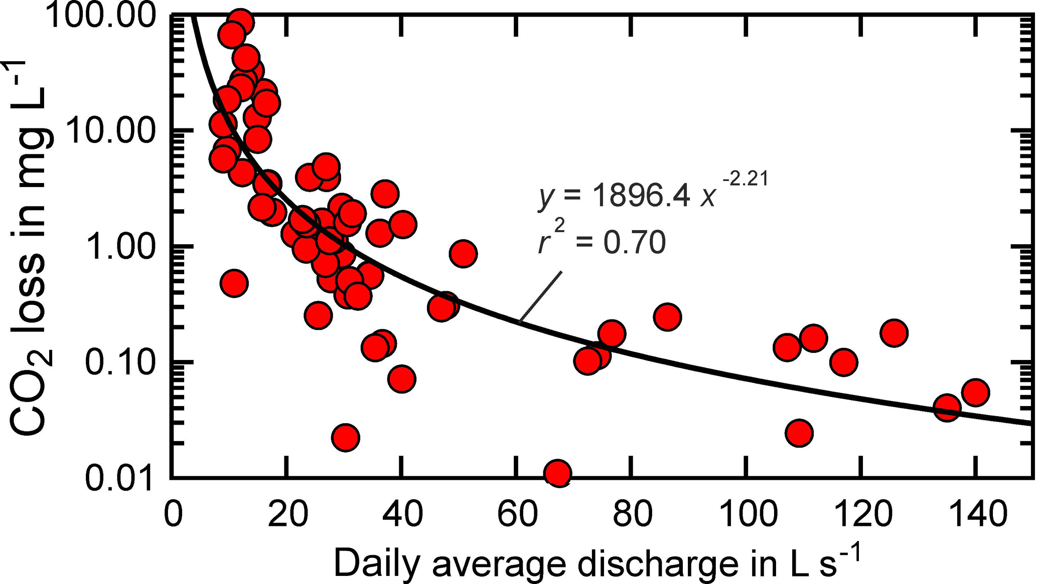
Figure 4Modelled CO2 loss via outgassing upstream of the measurement point (UHL) versus daily average discharge. Modelling results correspond to modelling with groundwater input.
Moreover, for CO2 loss ([DIC]ex) in mg C L−1 and daily average discharge in L s−1, a negative concentration–discharge relationship was observed (Fig. 4). Higher pCO2, modelled soil pCO2 and modelled CO2 loss occurred during low flow, when relative contributions of CO2-enriched groundwaters to stream waters were high. A similar concentration–discharge relationship was observed in a peatland stream, where deep soil and groundwater were considered as major CO2 sources (Dinsmore and Billett, 2008).
3.5 Export of DIC proportions
Measured DIC together with modelled CO2 outgassing from the stream surface to the atmosphere allowed the calculation of exported DIC species distributions. On an annual basis, the DIC proportions of export, CO (i.e. the sum of CO2(aq) and H2CO3) export, and CO2 outgassing had averages of 0.6, 1.2, and 7.1 to 10.3 mg C L−1 for CO2 outgassing with R=10 and 19 % (Table 3). This corresponds to the relative amounts of approximately % export, CO export, and CO2 outgassing with respect to total inorganic carbon loss from the Uhlířská catchment outlet.
For modelling with groundwater, the relative proportion of CO2 outgassing to annual DIC export was even higher. With concentrations of 0.6, 1.2, and 10.3 mg C L−1 of export, CO export, and CO2 outgassing they were approximately %. These values are comparable to relations found by other studies (Billett et al., 2004; Johnson et al., 2008; Davidson et al., 2010; Polsenaere and Abril, 2012) and largely differ from findings from a headwater stream in karstic bedrock, where < 30 % of DIC was outgassed as CO2 (Lee et al., 2017). The determined DIC proportions suggest that a very large proportion (> 80 %) of DIC entering the headwater stream in the silicate Uhlířská catchment rapidly outgasses as CO2.
Numerous studies have demonstrated the importance of CO2 outgassing from rivers and streams to the atmosphere on global carbon budgets and pointed out the restricted data on headwater catchments (Raymond et al., 2013; Lauerwald et al., 2015; Aufdenkampe et al., 2011). Here we present a new study that successfully applied, validated, and modified the CO2 degassing model by Polsenaere and Abril (2012) to a carbonate-free headwater catchment.
The modified isotope model was able to reproduce logical seasonal patterns of soil pCO2 with a high variability of soil pCO2 and CO2 outgassing. It showed increased fluxes in summer and during snowmelt in 2015. Modelled CO2 losses also negatively correlated with stream discharge. Results indicate maximum values of CO2 outgassing from the stream to the atmosphere shortly before snowmelt. Modelled annual CO2 outgassing was comparable to results obtained with model equations to calculate gas transfer velocities according to Raymond et al. (2012). However, results of the modified streamCO2-DEGAS model showed larger variability, which indicates its potential to assess temporal CO2 dynamics.
The model sensitivity to changing parameters of streamCO2-DEGAS model, such as the proportion of river respiration (R), in situ pCO2 and δ13CDIC, was high. This indicates that the potential to assess temporal variations becomes compromised by a larger potential for errors. This was particularly the case during summer.
Because of its decreased uncertainty, future CO2 modelling would further benefit from direct pCO2 measurement instead of its calculation. Such direct in situ methods include submerged infrared gas analysis (Johnson et al., 2010), equilibrator systems (Polsenaere et al., 2013), an off-axis integrated cavity output spectrometer combined with a gas analyser (Gonzalez-Valencia et al., 2014), and non-dispersive infrared sensors inside floating chambers (Bastviken et al., 2015; Lorke et al., 2015).
We circumvented the uncertainty of the respiration parameter (R) by incorporating wetland groundwater δ13CDIC into the model. By using groundwater data, the modelling results have shown substantial improvements when compared to modelling without groundwater data. We therefore stress the importance of adding more accurate groundwater measurements to such studies. This implies installation of more test wells in headwater catchments or the alternative use of local spring water as a proxy for groundwater. In addition, modelling at higher temporal resolution, particularly at the beginning of snowmelt, is needed to better reproduce dynamics and quantities of CO2 outgassing.
The data set is available at World Data Center PANGAEA https://doi.org/10.1594/PANGAEA.889689 (Marx et al., 2018).
The supplement related to this article is available online at: https://doi.org/10.5194/bg-15-3093-2018-supplement.
The authors declare that they have no conflict of interest.
This work was financially supported by the German Research Foundation (DFG,
project 718 BA 2207/10-1). The authors want to thank Pierre Polsenaere and
Gwenael Abril for advice and sharing their MATLAB code.
Edited by: Steven Bouillon
Reviewed by: two anonymous referees
Amiotte-Suchet, P., Aubert, D., Probst, J. L., Gauthier-Lafaye, F., Probst, A., Andreux, F., and Viville, D.: δ13C pattern of dissolved inorganic carbon in a small granitic catchment: the Strengbach case study (Vosges mountains, France), Chem. Geol., 159, 129–145, https://doi.org/10.1016/S0009-2541(99)00037-6, 1999.
Amundson, R. G. and Davidson, E. A.: Carbon-Dioxide and Nitrogenous Gases in the Soil Atmosphere, J. Geochem. Explor., 38, 13–41, https://doi.org/10.1016/0375-6742(90)90091-N, 1990.
Aufdenkampe, A. K., Mayorga, E., Raymond, P. A., Melack, J. M., Doney, S. C., Alin, S. R., Aalto, R. E., and Yoo, K.: Riverine coupling of biogeochemical cycles between land, oceans, and atmosphere, Front. Ecol. Environ., 9, 53–60, https://doi.org/10.1890/100014, 2011.
Barth, J. A. C., Mader, M., Nenning, F., van Geldern, R., and Friese, K.: Stable isotope mass balances versus concentration differences of dissolved inorganic carbon – implications for tracing carbon turnover in reservoirs, Isot. Environ. Healt. S., 13, 1–14, https://doi.org/10.1080/10256016.2017.1282478, 2017.
Bastviken, D., Sundgren, I., Natchimuthu, S., Reyier, H., and Galfalk, M.: Technical Note: Cost-efficient approaches to measure carbon dioxide (CO2) fluxes and concentrations in terrestrial and aquatic environments using mini loggers, Biogeosciences, 12, 3849–3859, https://doi.org/10.5194/bg-12-3849-2015, 2015.
Billett, M. F., Palmer, S. M., Hope, D., Deacon, C., Storeton-West, R., Hargreaves, K. J., Flechard, C., and Fowler, D.: Linking land-atmosphere-stream carbon fluxes in a lowland peatland system, Global Biogeochem. Cy., 18, 1–12, 2004.
Bishop, K., Buffam, I., Erlandsson, M., Folster, J., Laudon, H., Seibert, J., and Temnerud, J.: Aqua Incognita: the unknown headwaters, Hydrol. Process., 22, 1239–1242, https://doi.org/10.1002/Hyp.7049, 2008.
Boodoo, K. S., Trauth, N., Schmidt, C., Schelker, J., and Battin, T. J.: Gravel bars are sites of increased CO2 outgassing in stream corridors, Sci. Rep., 7, 1–9, https://doi.org/10.1038/s41598-017-14439-0, 2017.
Butman, D. and Raymond, P. A.: Significant efflux of carbon dioxide from streams and rivers in the United States, Nat. Geosci., 4, 839–842, https://doi.org/10.1038/Ngeo1294, 2011.
Campeau, A., Lapierre, J. F., Vachon, D., and del Giorgio, P. A.: Regional contribution of CO2 and CH4 fluxes from the fluvial network in a lowland boreal landscape of Quebec, Global Biogeochem. Cy., 28, 57–69, https://doi.org/10.1002/2013gb004685, 2014.
Catalan, N., Marce, R., Kothawala, D. N., and Tranvik, L. J.: Organic carbon decomposition rates controlled by water retention time across inland waters, Nat. Geosci., 9, 501–504, https://doi.org/10.1038/Ngeo2720, 2016.
Cole, J. J., Prairie, Y. T., Caraco, N. F., McDowell, W. H., Tranvik, L. J., Striegl, R. G., Duarte, C. M., Kortelainen, P., Downing, J. A., Middelburg, J. J., and Melack, J.: Plumbing the global carbon cycle: Integrating inland waters into the terrestrial carbon budget, Ecosystems, 10, 171–184, https://doi.org/10.1007/S10021-006-9013-8, 2007.
Coplen, T. B.: Guidelines and recommended terms for expression of stable-isotope-ratio and gas-ratio measurement results, Rapid Commun. Mass Spectrom., 25, 2538–2560, https://doi.org/10.1002/rcm.5129, 2011.
Crawford, J. T., Striegl, R. G., Wickland, K. P., Dornblaser, M. M., and Stanley, E. H.: Emissions of carbon dioxide and methane from a headwater stream network of interior Alaska, J. Geophys. Res.-Biogeo., 118, 482–494, https://doi.org/10.1002/Jgrg.20034, 2013.
Davidson, E. A., Figueiredo, R. O., Markewitz, D., and Aufdenkampe, A. K.: Dissolved CO2 in small catchment streams of eastern Amazonia: A minor pathway of terrestrial carbon loss, J. Geophys. Res.-Biogeo., 115, 1–6, https://doi.org/10.1029/2009jg001202, 2010.
Demars, B. O. L., Manson, J. R., Olafsson, J. S., Gislason, G. M., Gudmundsdottir, R., Woodward, G., Reiss, J., Pichler, D. E., Rasmussen, J. J., and Friberg, N.: Temperature and the metabolic balance of streams, Freshwater Biol., 56, 1106–1121, https://doi.org/10.1111/j.1365-2427.2010.02554.x, 2011.
Dickson, A. G., Sabine, C. L., and Christian, J. R. (Eds.): Guide to best practices for ocean CO2 measurements, PICES Special Publication 3, 191 pp., available at: https://www.nodc.noaa.gov/ocads/oceans/Handbook_2007.html (last access: 25 December 2018), 2007.
Dinsmore, K. J. and Billett, M. F.: Continuous measurement and modeling of CO2 losses from a peatland stream during stormflow events, Water Resour. Res., 44, W12417, https://doi.org/10.1029/2008wr007284, 2008.
Dusek, J., Vogel, T., and Sanda, M.: Hillslope hydrograph analysis using synthetic and natural oxygen-18 signatures, J. Hydrol., 475, 415–427, 2012.
Earth System Research Laboratory: National Oceanic and Atmospheric Administration/Earth System Research Laboratory-Global Monitoring Division (ESRL/GMD), Global average marine surface annual mean CO2 data, ESRL/GMD, Boulder, Colorado, available at: http://www.esrl.noaa.gov/gmd/index.html, last access: 10 July 2017.
Ehleringer, J. R. and Cerling, T. E.: C3 and C4 Photosynthesis, in: Encyclopedia of Global Environmental Change, Volume 2, The Earth System: Biological and Ecological Dimensions of Global Environmental Change, edited by: Mooney, H. A. and Canadell, J. G., John Wiley & Sons, 186–190, 2002.
Gonzalez-Valencia, R., Magana-Rodriguez, F., Gerardo-Nieto, O., Sepulveda-Jauregui, A., Martinez-Cruz, K., Anthony, K. W., Baer, D., and Thalasso, F.: In Situ Measurement of Dissolved Methane and Carbon Dioxide in Freshwater Ecosystems by Off-Axis Integrated Cavity Output Spectroscopy, Environ. Sci. Technol., 48, 11421–11428, https://doi.org/10.1021/Es500987j, 2014.
Halbedel, S. and Koschorreck, M.: Regulation of CO2 emissions from temperate streams and reservoirs, Biogeosciences, 10, 7539–7551, https://doi.org/10.5194/Bg-10-7539-2013, 2013.
Hotchkiss, E. R., Hall, R. O., Sponseller, R. A., Butman, D., Klaminder, J., Laudon, H., Rosvall, M., and Karlsson, J.: Sources of and processes controlling CO2 emissions change with the size of streams and rivers, Nat. Geosci., 8, 696–699, https://doi.org/10.1038/NGEO2507, 2015.
Hrncir, M., Sanda, M., Kulasova, A., and Cislerova, M.: Runoff formation in a small catchment at hillslope and catchment scales, Hydrol. Process., 24, 2248–2256, 2010.
Humborg, C., Morth, C. M., Sundbom, M., Borg, H., Blenckner, T., Giesler, R., and Ittekkot, V.: CO2 supersaturation along the aquatic conduit in Swedish watersheds as constrained by terrestrial respiration, aquatic respiration and weathering, Glob. Change Biol., 16, 1966–1978, https://doi.org/10.1111/J.1365-2486.2009.02092.X, 2010.
Huotari, J., Haapanala, S., Pumpanen, J., Vesala, T., and Ojala, A.: Efficient gas exchange between a boreal river and the atmosphere, Geophys. Res. Lett., 40, 5683–5686, https://doi.org/10.1002/2013GL057705, 2013.
Johnson, M. S., Lehmann, J., Riha, S. J., Krusche, A. V., Richey, J. E., Ometto, J. P. H. B., and Couto, E. G.: CO2 efflux from Amazonian headwater streams represents a significant fate for deep soil respiration, Geophys. Res. Lett., 35, 1–5, https://doi.org/10.1029/2008gl034619, 2008.
Johnson, M. S., Billett, M. F., Dinsmore, K. J., Wallin, M., Dyson, K. E., and Jassal, R. S.: Direct and continuous measurement of dissolved carbon dioxide in freshwater aquatic systems-method and applications, Ecohydrology, 3, 68–78, https://doi.org/10.1002/Eco.95, 2010.
Jones, J. B. and Mulholland, P. J.: Influence of drainage basin topography and elevation on carbon dioxide and methane supersaturation of stream water, Biogeochemistry, 40, 57–72, https://doi.org/10.1023/A:1005914121280, 1998.
Lauerwald, R., Laruelle, G. G., Hartmann, J., Ciais, P., and Regnier, P. A. G.: Spatial patterns in CO2 evasion from the global river network, Global Biogeochem. Cy., 29, 534–554, https://doi.org/10.1002/2014GB004941, 2015.
Lee, K. Y., van Geldern, R., and Barth, J. A. C.: A high-resolution carbon balance in a small temperate catchment: Insights from the Schwabach River, Germany, Appl. Geochem., 85, 86–96, https://doi.org/10.1016/j.apgeochem.2017.08.007, 2017.
Lorke, A., Bodmer, P., Noss, C., Alshboul, Z., Koschorreck, M., Somlai-Haase, C., Bastviken, D., Flury, S., McGinnis, D. F., Maeck, A., Muller, D., and Premke, K.: Technical note: drifting versus anchored flux chambers for measuring greenhouse gas emissions from running waters, Biogeosciences, 12, 7013–7024, https://doi.org/10.5194/bg-12-7013-2015, 2015.
Marx, A., Dusek, J., Jankovec, J., Sanda, M., Vogel, T., van Geldern, R., Hartmann, J., and Barth, J. A. C.: A review of CO2 and associated carbon dynamics in headwater streams: A global perspective, Rev. Geophys., 55, 560–585, https://doi.org/10.1002/2016RG000547, 2017a.
Marx, A., Hintze, S., Sanda, M., Jankovec, J., Oulehle, F., Dusek, J., Vogel, T., Vitvar, T., van Geldern, R., and Barth, J. A. C.: Acid rain footprint three decades after peak deposition: Long-term recovery from pollutant sulphate in the Uhlirska catchment (Czech Republic), Sci. Total. Env., 598, 1037–1049, https://doi.org/10.1016/j.scitotenv.2017.04.109, 2017b.
Marx, A., Conrad, M., Aizinger, V., Prechtel, A., van Geldern, R., and Barth, J. A. C.: Stream and groundwater chemistry of the Uhlirska catchment, Czech Republic, PANGAEA, https://doi.org/10.1594/PANGAEA.889689, 2018.
Mook, W. G., Bommerso, J. C., and Staverma, W. H.: Carbon Isotope Fractionation between Dissolved Bicarbonate and Gaseous Carbon-Dioxide, Earth Plan. Sc. Lett., 22, 169–176, https://doi.org/10.1016/0012-821x(74)90078-8, 1974.
Mook, W. G., Koopmans, M., Carter, A. F., and Keeling, C. D.: Seasonal, Latitudinal, and Secular Variations in the Abundance and Isotopic-Ratios of Atmospheric Carbon-Dioxide.1. Results from Land Stations, J. Geophys. Res.-Oc. Atm., 88, 915–933, https://doi.org/10.1029/Jc088ic15p10915, 1983.
Moran, M. A. and Zepp, R. G.: Role of photoreactions in the formation of biologically labile compounds from dissolved organic matter, Limnol. Oceanogr., 42, 1307–1316, 1997.
Myrttinen, A., Becker, V., and Barth, J. A. C.: A review of methods used for equilibrium isotope fractionation investigations between dissolved inorganic carbon and CO2, Earth-Sci. Rev., 115, 192–199, https://doi.org/10.1016/j.earscirev.2012.08.004, 2012.
Myrttinen, A., Becker, V., and Barth, J. A. C.: Corrigendum to “A review of methods used for equilibrium isotope fractionation investigations between dissolved inorganic carbon and CO2” (Earth Sci. Rev., 115, 192–199), Earth-Sci. Rev., 141, 178–178, https://doi.org/10.1016/j.earscirev.2014.11.009, 2015.
O'Leary, M. H.: Measurement of the isotope fractionation associated with diffusion of carbon dioxide in aqueous solution, J. Phys. Chem.-US, 88, 823–825, 1984.
Pacific, V. J., McGlynn, B. L., Riveros-Iregui, D. A., Welsch, D. L., and Epstein, H. E.: Variability in soil respiration across riparian-hillslope transitions, Biogeochemistry, 91, 51–70, https://doi.org/10.1007/s10533-008-9258-8, 2008.
Plummer, L. N. and Busenberg, E.: The Solubilities of Calcite, Aragonite and Vaterite in CO2-H2O Solutions between 0 and 90 ∘C, and an Evaluation of the Aqueous Model for the System CaCO3-CO2-H2O, Geochim. Cosmochim. Ac., 46, 1011–1040, https://doi.org/10.1016/0016-7037(82)90056-4, 1982.
Polsenaere, P. and Abril, G.: Modelling CO2 degassing from small acidic rivers using water pCO2, DIC and δ13C-DIC data, Geochim. Cosmochim. Ac., 91, 220–239, https://doi.org/10.1016/J.Gca.2012.05.030, 2012.
Polsenaere, P., Savoye, N., Etcheber, H., Canton, M., Poirier, D., Bouillon, S., and Abril, G.: Export and degassing of terrestrial carbon through watercourses draining a temperate podzolized catchment, Aquat. Sci., 75, 299–319, https://doi.org/10.1007/S00027-012-0275-2, 2013.
Raymond, P. A., Zappa, C. J., Butman, D., Bott, T. L., Potter, J., Mulholland, P., Laursen, A. E., McDowell, W. H., and Newbold, D.: Scaling the gas transfer velocity and hydraulic geometry in streams and small rivers, Limnol. Oceanogr.-Fluids Environ., 2, 41–53, https://doi.org/10.1215/21573689-1597669, 2012.
Raymond, P. A., Hartmann, J., Lauerwald, R., Sobek, S., McDonald, C., Hoover, M., Butman, D., Striegl, R., Mayorga, E., Humborg, C., Kortelainen, P., Durr, H., Meybeck, M., Ciais, P., and Guth, P.: Global carbon dioxide emissions from inland waters, Nature, 503, 355–359, https://doi.org/10.1038/Nature12760, 2013.
Raymond, P. A., Saiers, J. E., and Sobczak, W. V.: Hydrological and biogeochemical controls on watershed dissolved organic matter transport: pulse-shunt concept, Ecology, 97, 5–16, https://doi.org/10.1890/14-1684.1, 2016.
Regnier, P., Friedlingstein, P., Ciais, P., Mackenzie, F. T., Gruber, N., Janssens, I. A., Laruelle, G. G., Lauerwald, R., Luyssaert, S., Andersson, A. J., Arndt, S., Arnosti, C., Borges, A. V., Dale, A. W., Gallego-Sala, A., Godderis, Y., Goossens, N., Hartmann, J., Heinze, C., Ilyina, T., Joos, F., LaRowe, D. E., Leifeld, J., Meysman, F. J. R., Munhoven, G., Raymond, P. A., Spahni, R., Suntharalingam, P., and Thullner, M.: Anthropogenic perturbation of the carbon fluxes from land to ocean, Nat. Geosci., 6, 597–607, https://doi.org/10.1038/ngeo1830, 2013.
Reichert, P., Uehlinger, U., and Acuna, V.: Estimating stream metabolism from oxygen concentrations: Effect of spatial heterogeneity, J. Geophys. Res.-Biogeo., 114, G03016, https://doi.org/10.1029/2008jg000917, 2009.
Sanda, M. and Cislerova, M.: Transforming Hydrographs in the Hillslope Subsurface, J. Hydrol. Hydromech., 57, 264–275, https://doi.org/10.2478/V10098-009-0023-Z, 2009.
Sanda, M., Vitvar, T., Kulasova, A., Jankovec, J., and Cislerova, M.: Run-off formation in a humid, temperate headwater catchment using a combined hydrological, hydrochemical and isotopic approach (Jizera Mountains, Czech Republic), Hydrol. Process., 28, 3217–3229, https://doi.org/10.1002/hyp.9847, 2014.
Sawakuchi, H. O., Neu, V., Ward, N. D., Barros, M. d. L. C., Valerio, A. M., Gagne-Maynard, W., Cunha, A. C., Less, D. F. S., Diniz, J. E. M., Brito, D. C., Krusche, A. V., and Richey, J. E.: Carbon Dioxide Emissions along the Lower Amazon River, Front. Mar. Sci., 4, 1–12, https://doi.org/10.3389/fmars.2017.00076, 2017.
Schelker, J., Singer, G. A., Ulseth, A. J., Hengsberger, S., and Battin, T. J.: CO2 evasion from a steep, high gradient stream network: importance of seasonal and diurnal variation in aquatic pCO2 and gas transfer, Limnol. Oceanogr., 61, 1826–1838, https://doi.org/10.1002/lno.10339, 2016.
St-Jean, G.: Automated quantitative and isotopic (13C) analysis of dissolved inorganic carbon and dissolved organic carbon in continuous-flow using a total organic carbon analyser, Rapid Commun. Mass Spectrom., 17, 419–428, https://doi.org/10.1002/rcm.926, 2003.
Stets, E. G., Butman, D., McDonald, C. P., Stackpoole, S. M., DeGrandpre, M. D., and Striegl, R. G.: Carbonate buffering and metabolic controls on carbon dioxide in rivers, Global Biogeochem. Cy., 31, 663–677, https://doi.org/10.1002/2016gb005578, 2017.
Teodoru, C. R., Del Giorgio, P. A., Prairie, Y. T., and Camire, M.: Patterns in pCO2 in boreal streams and rivers of northern Quebec, Canada, Global Biogeochem. Cy., 23, 1–11, https://doi.org/10.1029/2008gb003404, 2009.
van Geldern, R., Schulte, P., Mader, M., Baier, A., and Barth, J. A. C.: Spatial and temporal variations of pCO2, dissolved inorganic carbon, and stable isotopes along a temperate karstic watercourse, Hydrol. Process., 29, 3423–3440, https://doi.org/10.1002/hyp.10457, 2015.
Venkiteswaran, J. J., Schiff, S. L., and Wallin, M. B.: Large Carbon Dioxide Fluxes from Headwater Boreal and Sub-Boreal Streams, Plos One, 9, 1–9, https://doi.org/10.1371/journal.pone.0101756, 2014.
Vitvar, T., Sanda, M., Marx, A., Hubert, E., Jankovec, J., and Barth, J. A. C.: Hydrochemical and isotopic tracing of runoff generation in the small mountainous catchment Uhlirska (Czech Republic), using the NETPATH approach, Acta Hydrologica Slovaca, 17, 190–198, 2016.
Vogel, J. C.: Variability of Carbon Isotope Fractionation during Photosynthesis, in: Stable Isotopes and Plant Carbon-water Relations, edited by: Ehleringer, J. R., Hall, A. E., and Farquhar, G. D., Academic Press, San Diego, 29–46, ISBN 9780122333804, https://doi.org/10.1016/B978-0-08-091801-3.50010-6, 1993,
Wallin, M. B., Oquist, M. G., Buffam, I., Billett, M. F., Nisell, J., and Bishop, K. H.: Spatiotemporal variability of the gas transfer coefficient ( in boreal streams: Implications for large scale estimates of CO2 evasion, Global Biogeochem. Cy., 25, 1–14, https://doi.org/10.1029/2010gb003975, 2011.
Wehrli, B.: Biogeochemistry Conduits of the Carbon Cycle, Nature, 503, 346–347, 2013.