the Creative Commons Attribution 3.0 License.
the Creative Commons Attribution 3.0 License.
Can land degradation drive differences in the C exchange of two similar semiarid ecosystems?
Ana López-Ballesteros
Cecilio Oyonarte
Andrew S. Kowalski
Penélope Serrano-Ortiz
Enrique P. Sánchez-Cañete
M. Rosario Moya
Francisco Domingo
Currently, drylands occupy more than one-third of the global terrestrial surface and are recognized as areas vulnerable to land degradation. The concept of land degradation stems from the loss of an ecosystem's biological productivity due to long-term loss of natural vegetation or depletion of soil nutrients. Drylands' key role in the global carbon (C) balance has been recently demonstrated, but the effects of land degradation on C sequestration by these ecosystems still need to be investigated. In the present study, we compared net C and water vapor fluxes, together with satellite, meteorological and vadose zone (CO2, water content and temperature) measurements, between two nearby (∼ 23 km) experimental sites representing “natural” (i.e., site of reference) and “degraded” grazed semiarid grasslands. We utilized data acquired over 6 years from two eddy covariance stations located in southeastern Spain with highly variable precipitation magnitude and distribution. Results show a striking difference in the annual C balances with an average net CO2 exchange of 196 ± 40 (C release) and −23 ± 2 g C m−2 yr−1 (C fixation) for the degraded and natural sites, respectively. At the seasonal scale, differing patterns in net CO2 fluxes were detected over both growing and dry seasons. As expected, during the growing seasons, greater net C uptake over longer periods was observed at the natural site. However, a much greater net C release, probably derived from subterranean ventilation, was measured at the degraded site during drought periods. After subtracting the nonbiological CO2 flux from net CO2 exchange, flux partitioning results point out that, during the 6 years of study, gross primary production, ecosystem respiration and water use efficiency were, on average, 9, 2 and 10 times higher, respectively, at the natural site versus the degraded site. We also tested differences in all monitored meteorological and soil variables and CO2 at 1.50 m belowground was the variable showing the greatest intersite difference, with ∼ 1000 ppm higher at the degraded site. Thus, we believe that subterranean ventilation of this vadose zone CO2, previously observed at both sites, partly drives the differences in C dynamics between them, especially during the dry season. It may be due to enhanced subsoil–atmosphere interconnectivity at the degraded site.
- Article
(2550 KB) -
Supplement
(269 KB) - BibTeX
- EndNote


The concept of land degradation stems from the loss of an ecosystem's biological productivity, which in turn relies on several degradation processes such as long-term loss of natural vegetation, deterioration of soil quality, biodiversity depletion or water and wind erosion (UNCCD, 1994). Drylands (arid, semiarid and dry subhumid areas), which occupy more than one-third of Earth's land surface and are inhabited by more than 2 billion people (Niemeijer et al., 2005), have been recognized as areas vulnerable to land degradation processes. In fact, they have expanded globally for the last 60 years at an estimated annual rate of 5.8 million ha in midlatitudes alone (Lal, 2001) and are projected to expand under future climate change scenarios (Feng and Fu, 2013; Cook et al., 2014), especially in the Mediterranean region, where major expansions of semiarid areas will occur (Gao and Giorgi, 2008; Feng and Fu, 2013).
Over recent decades, most research focused on land degradation has been based on remote sensing and Earth observation techniques. Much of these investigations have aimed to refine methodological issues in order to accurately track land degradation in vulnerable areas, reduce uncertainties and explain inconsistencies among studies. For instance, a wide array of satellite-derived data, such as vegetation indices, normalized surface reflectance, brightness temperature or biomass net primary production derivatives (Mbow et al., 2015), have been utilized to appraise desertification effects in the Sahel (Mbow et al., 2015; Fensholt et al., 2013) and also in other African countries such as Kenya (Omuto, 2011), Somalia (Omuto et al., 2010), South Africa (Thompson et al., 2009) or Zimbabwe (Prince et al., 2009). Likewise, desertification in the Mediterranean region has been studied through satellite imagery in Greece (Bajocco et al., 2012), Israel (Shoshany and Karnibad, 2015) and the Iberian Peninsula (del Barrio et al., 2010). However, although drylands' key role in the global carbon (C) balance has been demonstrated (Poulter et al., 2014; Ahlström et al., 2015), very few investigations have directly quantified how land degradation processes disturb the C sequestration capacity of drylands (Lal, 2001), despite it being one of the most important ecosystem services (Watanabe and Ortega, 2011).
In this regard, the few C-related desertification studies conducted over the last decade have centered on soil C dynamics. In particular, soil organic carbon (SOC) inventories have been used to explore the effects of climate, human activities and grazing pressure in desertification-prone areas of China (Feng et al., 2006) and Brazil (Schulz et al., 2016). Similarly, other investigations have evaluated soil degradation processes by means of soil CO2 effluxes together with other biometric measurements in drylands found in China (Hou et al., 2014; Wang et al., 2007), Chile (Bown et al., 2014) and southeastern Spain (Rey et al., 2011, 2017). However, the degradation processes associated with desertification affect several subsystems as well as their interactions at multiple spatial and temporal scales. For instance, adverse effects on soil quality involve depletion of soil fertility, but also reduce soil–water storage (Mainguet and Da Silva, 1998), which, in turn, can constrain seed germination and vegetation reestablishment, modify climax vegetation, disrupt biogeochemical cycles, alter water and energy balances, and consequently lead to a loss of ecosystem resilience (Lal, 2001). This cascade of disturbances may result in a reduction of the C sequestration capacity of a given ecosystem, which is clearly a symptom of the loss of biological productivity, resulting in a positive feedback to global warming. Therefore, a quite suitable and holistic approach is to integrate all subsystem effects into a whole ecosystem-scale assessment when quantifying the C loss derived from land degradation. However, the use of this integrative method is mostly lacking in the available literature.
The present study is located in the southeast of Spain, which has been recognized as a hotspot of land degradation owing to the synergistic interaction of sociological and climatic factors (Puigdefábregas and Mendizabal, 1998). Our core aim is to evaluate how dryland degradation affects the dynamics of net ecosystem–atmosphere C exchange of two semiarid grasslands that represent differing degradation statuses (natural versus degraded) by means of meteorological, satellite and subsoil CO2 measurements together with carbon and water fluxes acquired by the eddy covariance (EC) technique (Baldocchi et al., 1988). Owing to the high temporal resolution of the EC method, we can assess the effect of land degradation as a slow change or disturbance legacy in the studied ecosystems and how, in turn, it influences the ecosystems' resilience against short-term disturbances, such as climate extremes (i.e., droughts, heatwaves).
Some land degradation processes are evident when we compare the natural site with the degraded site. Accordingly, our main hypothesis is that land degradation processes can directly affect abiotic and/or biotic factors and consequently influence the biological and/or nonbiological processes that compose the net ecosystem CO2 exchange: gross primary production, ecosystem respiration and subterranean ventilation – a nonbiological process that provokes the transfer of CO2-rich air from the subsoil to the atmosphere under drought and high-turbulence conditions. Firstly, the lower vegetation cover at the degraded site would entail a higher thermal and radiative stress at the surface, especially during the drought period (Rey et al., 2017). The hypothesized effects on biological processes are a direct reduction in plant productivity and respiration, and an indirect decrease in heterotrophic respiration. Secondly, the higher cover of bare soil and outcrops at the degraded site may increase the soil–atmosphere interconnectivity, which can indirectly enhance the presence of advective CO2 release through subterranean ventilation, which has been previously measured at both experimental sites (Rey et al., 2012a; López-Ballesteros et al., 2017). Thirdly, the reduced soil fertility and depth may provoke changes in microbial communities (Evans and Wallenstein, 2014) due to stronger nutrient and water limitations. Consequently, a direct decrease in heterotrophic respiration and plant productivity and respiration is expected.
Hence, our specific objectives are (1) to compare the C sequestration capacity of two semiarid ecosystems with differing degradation status, (2) to study the underlying processes (biological versus nonbiological) and influencing factors that can drive potential differences in the net C exchange of studied ecosystems, and (3) to evaluate whether degradation can modulate ecosystem responses against short-term disturbances.
In this study, we analyzed 12 site-years of EC data, enhanced vegetation index (EVI) time series and monitored ambient variables registered over the same period (2009–2015) at two experimental sites. Additionally, we used subsoil CO2, moisture and temperature data obtained during 2014–2015.
2.1 Experimental site description
The study area is located in southeastern Spain, the driest part of Europe. The two experimental sites, Amoladeras (36∘50′5 M, 2∘15′1 W) and Balsa Blanca (36∘56′26.0 N, 2∘01′58.8 W), are found within the Cabo de Gata-Níjar Natural Park (Almería, Spain; Fig. 1) and are quite similar in terms of climate and ecosystem type. Both sites show a desert climate, according to the Köppen classification (Bwh; Kottek et al., 2006), with a mean annual temperature of 18 ∘C and mean annual precipitation of approximately 220 mm.
The ecosystem type corresponds to espartal, a Mediterranean semiarid grassland where the dominant species is Machrochloa tenacissima. This ecosystem type is widespread in the western Mediterranean region: in Cabo de Gata-Níjar Natural Park, a large fraction of agricultural areas that were abandoned over 1957–1994 resulted in espartal ecosystems (Alados et al., 2004, 2011). The functioning of both experimental sites can be divided into two main periods. On one hand, the growing season usually extends from late autumn to early spring, when the temperature starts to rise and water resources have not yet become scarce (López-Ballesteros et al., 2016; Serrano-Ortiz et al., 2014). On the other hand, a long period of hydric stress, with high temperatures and scarce precipitation, results in a prolonged dry season that usually begins in May–June and ends in September–October, when the first autumn rainfall events occur. Additionally, water inputs derived from relevant dewfall episodes, which have been previously reported in the area (Uclés et al., 2014), can rehydrate soil and plants at night and in the early morning hours.
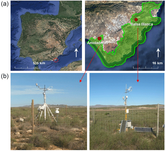
Figure 1Location (a) and photographs (b) of the experimental sites. Green area represents the Cabo de Gata-Níjar Natural Park (Almería, Spain).
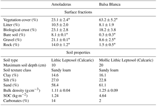
Regarding the topographic, geologic and edaphic characteristics, both sites are located on an alluvial fan, where the main geological materials consist of quaternary conglomerates and Neogene–Quaternary sediments cemented by lime (caliche) (Rodríguez-Fernández et al., 2015) on slopes of 2–6 % (Rey et al., 2017), so no significant runoff occurs. Additionally, both sites present petrocalcic horizons. However, altitude and soil type differ. While Balsa Blanca (hereinafter BB) is located at an altitude of 208 m and has Mollic and Lithic Leptosols (Calcaric), Amoladeras (hereinafter AMO) is situated closer to sea level, at 65 m and presents less developed soils Lithic Leptosol (Calcaric; Table 1).
Overall, as stated by Rey et al. (2011), these two experimental sites represent different degradation stages owing to their differing soil characteristics and surface fractions (Table 1). While BB has deeper and more fertile soils and higher vegetation cover, AMO shows thinner and poorer soils and has half of Balsa Blanca's vegetation cover. Therefore, in accordance with Rey et al. (2011, 2017), we considered that BB represents the natural site, currently being a representative ecosystem of the area, while AMO represents a degraded site with respect to BB. The stronger degradation effects observed in AMO (degraded site) compared to BB (natural site) are probably due to its proximity to populated areas. The main factor provoking degradation in this Mediterranean area was the increase in rural population from the beginning of the 20th century to the late 1950s (Grove and Rackham, 2001). At that time, timber extraction and the use of tussock fiber for textile manufacturing and extensive farming were common economic activities that likely increased anthropic pressure on the degraded site. Afterwards, rural exodus during the middle of the century involved the abandonment of these agriculture practices. However, although degradation drivers are not currently active, their effects are still observable in the area corresponding to a case of “relict” degradation (Puigdefábregas and Mendizábal, 2004).
Table 1Site characteristics, surface fractions and soil properties of both experimental sites studied. Asterisks denote significant differences (p-value < 0.05). Adapted from Rey et al. (2011).
2.2 Meteorological and eddy covariance measurements
The net ecosystem–atmosphere exchange of water vapor, CO2 and sensible and latent heat were measured in terms of fluxes via the EC technique. Thus, an EC station was installed at each experimental site, AMO and BB (with site codes Es-Amo and Es-Agu of the European Fluxes Database Cluster http://www.europe-fluxdata.eu), where ambient and micrometeorological variables (detailed in Table 2) were monitored continuously since 2009. The EC footprint (i.e., actual measured area) is well within the fetch (i.e., distance to a change in surface characteristics) at both sites. Regarding data processing, the half-hourly averaged fluxes were calculated from raw data collected at 10 Hz using EddyPro 5.1.1 software (Li-Cor, Inc., USA). Flux calculation, flux corrections and quality assessment were performed according to López-Ballesteros et al. (2016).
Additionally, flux measurements acquired under low-turbulence conditions were excluded from the analysis by using a friction velocity (u*) threshold according to the approach proposed by Reichstein et al. (2005). The average u* thresholds for the entire study period (i.e., 2009–2015) were 0.11 and 0.16 m s−1, for AMO and BB. Therefore, the total annual fractions of missing half-hourly net CO2 fluxes accounted for 33 ± 3 and 29 ± 6 % of nighttime data and 8 ± 6 and 14 ± 5 % of daytime data, for AMO and BB, respectively. Missing data were gap-filled by means of the marginal distribution approach proposed by Reichstein et al. (2005) and uncertainty derived from the gap-filling procedure was calculated by using the variance of the measured data, which were calculated by introducing artificial gaps and repeating the standard gap-filling procedure. Twice the standard deviation of sums of total data were taken as the uncertainty for the several aggregating time periods we used in the analysis. The annual cumulative C balance was estimated, when possible, by integrating gap-filled half-hourly net CO2 fluxes of good quality (0 and 1 quality flags, according to Mauder and Foken, 2004) over a hydrological year.
In order to test the validity of both EC stations, we assessed the energy balance closure (Moncrieff et al., 1997) by computing the linear regression of half-hourly turbulent energy fluxes (sensible and latent heat fluxes; H + LE; W m−2) against available energy (net radiation less the soil heat flux; Rn − G; W m−2) using the whole of the 6-year database. The storage term in the soil heat flux was included in the estimates, while in the cases of sensible and latent heat fluxes, this term was negligible given the short height of the vegetation (∼ 50 cm). The resulting slopes were 0.873 ± 0.002 (R2 = 0.907) and 0.875 ± 0.001 (R2 = 0.920) for AMO and BB, respectively.
Table 2Variables measured, sensors used and their installation height in Amoladeras and Balsa Blanca experimental sites.
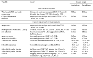
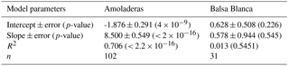
Table 3Linear regression results between half-hourly net CO2 fluxes of maximum quality (QC flag = 0) and friction velocity (u*) used to model subterranean ventilation.
2.3 Flux partitioning
In order to partition net CO2 ecosystem exchange into gross primary production (GPP) and ecosystem respiration (Reco), we first modeled the ventilative CO2 efflux by adapting the approach proposed by Pérez-Priego et al. (2013) using the results of previous studies at both sites (López-Ballesteros et al., 2016, 2017). Essentially, we aimed to isolate those moments when subterranean ventilation (Vn) dominates the net CO2 fluxes (Fc) and biological fluxes are negligible. These moments correspond to daytime hours during the extremely dry periods. Accordingly, data were selected using the following conditions: (i) net radiation > 10 W m−2, (ii) 8 < daily averaged Bowen ratio < 10, and (iii) daily soil water content (in bare soil) < 10th percentile (in AMO) and < 20th percentile (in BB). A less restrictive threshold was used in BB in order to get enough data to build the Vn model, since long-term data gaps occurred at this site during the summer seasons of 2012, 2014 and 2015. Afterwards, in order to build the linear model of Vn, these selected Fc data (maximum quality; QC flag = 0) were related to the friction velocity (u*).
As the results show (Table 3; Fig. S1 in the Supplement), the Vn model is uniquely valid for AMO. Therefore, we only applied the Vn model to AMO data, particularly during those periods when ventilation (but not exclusively) occurs according to previous research (López-Ballesteros et al., 2017). Hence, the model was applied when (i) net radiation > 10 W m−2, (ii) daily averaged Bowen ratio > 4, (iii) daily soil water content (in bare soil) < 0.01 m3 m−3, and (iv) σswc (daily variance of soil water content in bare soil) < 5 × 10⁻⁶ (m3 m−3)2. We use those moments with very low σswc in order to discern Reco increases caused by rain pulses (Birch effect) from Vn fluxes during the dry season. Then, the modeled ventilative fluxes were subtracted from the measured net CO2 exchange to obtain the CO2 flux corresponding only to biological processes (i.e., biological Fc; see Fig. S2).
Finally, the partitioning approach proposed by Lasslop et al. (2010) was applied to the biological Fc for both sites in order to obtain GPP and Reco fluxes. We chose this approach given the determinant influence of hydric stress, in this case atmospheric drought (assessed via VPD), on the physiology of Machrochloa tenacissima, the dominant plant species of the studied semiarid ecosystems (Pugnaire et al., 1996; López-Ballesteros et al., 2016).
2.4 Enhanced vegetation index data series
We used EVI data acquired by the Moderate Resolution Imaging Spectroradiometer (MODIS), which is on board the Earth Observing System-Terra platform, in order to track vegetation dynamics at both experimental sites. The nominal resolution of EVI products (code MOD13Q1) is 250 m at nadir and temporal resolution corresponds to 16-day compositing periods. The spatial coordinates used for AMO and BB were 36.8340∘ N, −2.2526∘ E and 36.9394∘ N, −2.0341∘ E, respectively.
2.5 Vadose zone measurements
Subsoil CO2 molar fraction, temperature and volumetric water content were measured at 0.05 and 1.50 m below the surface (Table 2) from January 2014 to August 2015 at both experimental sites. In the case of the shallower CO2 sensor, it was installed vertically with an in-soil adapter (211921GM, Vaisala, Inc., Finland) to avoid water entering. Subsoil CO2 molar fractions were sampled every 30 s and 5 min averages were stored in a data logger (CR3000 and CR1000, CSI; for AMO and BB, respectively). The deeper CO2 sensor was equipped with a soil adapter for horizontal positioning (215519, Vaisala, Inc., Finland) and consisted of a PTFE filter to protect to the CO2 sensor from water. It was buried in the summer of 2013 and the measurements were made every 30 s and stored as 5 min averages in a data logger (CR1000 and CR23X Campbell Sci., Logan, UT, USA, for AMO and BB, respectively). All CO2 molar fraction records were corrected for variations in soil temperature and atmospheric pressure.
2.6 Statistical analysis
All meteorological and soil variables monitored at each site were compared through computation of the nonparametric two-sided Wilcoxon summed rank test in order to detect those factors/variables influencing potentially distinct ecosystem functioning between sites. This test was chosen because the variables used satisfied the independence and continuity assumptions but not all were normally distributed. The confidence level used was 95 %. The effect size was evaluated using the median of the difference between the samples (AMO minus BB), which was expressed as a standardized value (divided by its standard deviation; Diffst; dimensionless) in order to be able to compare results among different variables. This analysis was performed by using three different periods: the entire study period, the period from May to September and the period from May to September only during the daytime. These periods were selected given their demonstrated coincidence with high relevance of nonbiological processes. All calculations were performed using R software version 3.2.5.
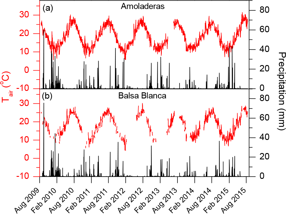
Figure 2Daily averages of air temperature (Tair) and precipitation in (a) Amoladeras and (b) Balsa Blanca.
Additionally, in order to include the relationship between pressure and subsoil CO2 variations as a potential factor influencing net CO2 exchange (Sánchez-Cañete et al., 2013), we first calculated, separately for each site, Spearman correlation coefficients to determine the time step (6, 12, 24 or 72 h) with the highest correlation between the differential transformation of pressure and the subsoil CO2 molar fraction at 1.50 m.
3.1 Ambient conditions
Over the study period, the wettest hydrological year was 2009–2010, with an annual precipitation of ∼ 500 mm (ca. twice the mean annual precipitation for both sites over the study period, Fig. 2). In contrast, the driest year was 2013–2014, with an annual precipitation of ∼ 100 mm for both sites, less than half the annual average precipitation registered at AMO and BB. Generally, months with precipitation exceeding 20 mm occurred from the beginning of autumn to midwinter. However, in 2009–2010, 2010–2011, 2012–2013 and 2014–2015, relevant rain events were registered during the spring months. By contrast, in 2013–2014, precipitation was always below 20 mm with the exception of November and December, for both sites, and June, in the case of AMO (Fig. 2a). Commonly, while maximum precipitation usually occurred from November to February, there was a remarkable drought period over the summer months (June–August) when it scarcely ever rained (Fig. 2).
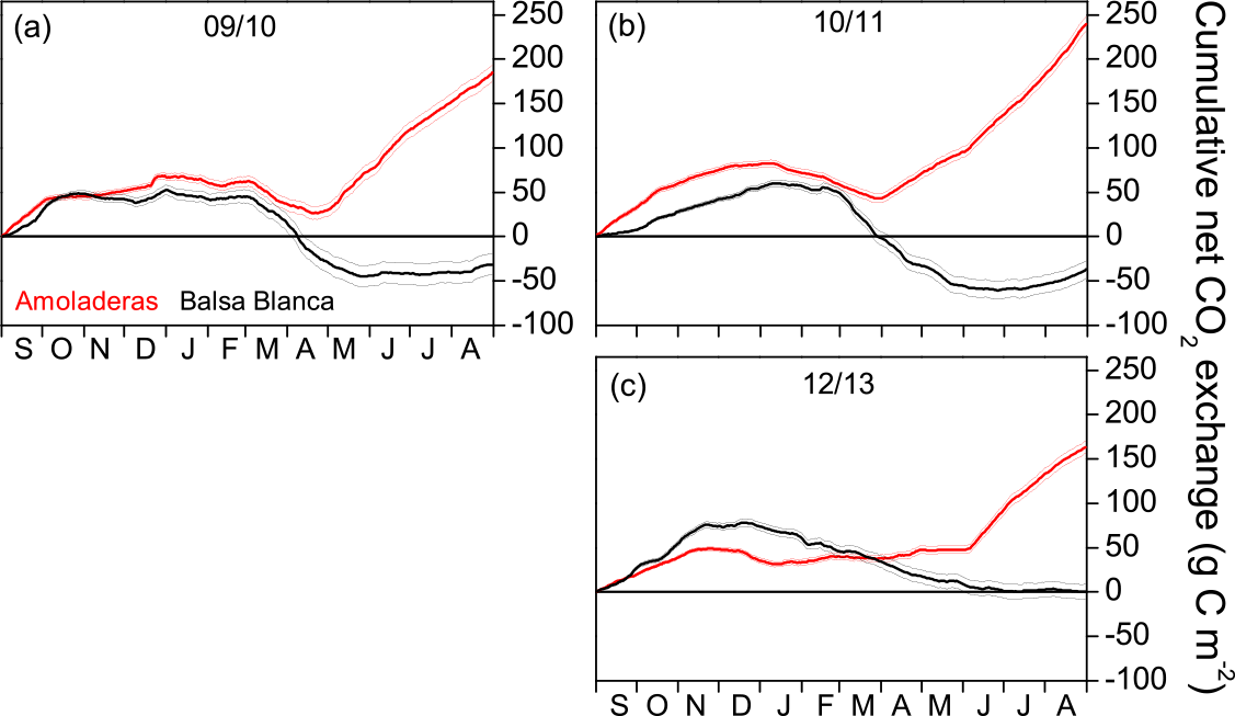
Figure 3Cumulative annual net CO2 exchange over the 3 hydrological years without long periods of missing data at both experimental sites, Amoladeras (red lines) and Balsa Blanca (black lines). Negative values denote net carbon uptake, while positive values denote net carbon release. Thin lines indicate uncertainty derived from the gap-filling procedure.
Regarding air temperature (Tair) patterns, monthly averaged Tair ranged from 9.6 and 8.1 ∘C to 27.6 and 27.9 ∘C in AMO and BB, respectively, over the entire study period. Based on half-hourly averaged data, minimum and maximum Tair values registered were 0.1 and 37.9 ∘C in AMO, and −1.3 and 39.9 ∘C, in BB, respectively. On one hand, those months with Tair above 15 ∘C usually corresponded approximately to April–November. Additionally, August was the month with the highest average Tair at both sites, with Tair ranges of 25.2–27.6 ∘C at AMO and 24.9–27.9 ∘C at BB, respectively (Fig. 2), over the study period. On the other hand, the lowest monthly average Tair usually occurred in January but sometimes also in December and February, with 11.2–12.3 ∘C at AMO and 8.1–14.1 ∘C at BB.
3.2 Annual carbon balances
The comparison of the annual C balance among sites was only possible for 3 hydrological years, 2009–2010, 2010–2011 and 2012–2013, due to long-term data gaps existing in BB during other years. The annual cumulative net CO2 exchange was always positive for AMO (i.e., net C release), whereas BB was neutral or even acted as a C sink over the 3 years (Fig. 3). For example, in 2009–2010, the net C uptake measured in BB equated to 32 ± 10 g C m−2, while in AMO, a total amount of 185 ± 10 g C m−2 was released into the atmosphere (Fig. 3a). The year with the largest difference between sites was 2010–2011, with an annual C release of 240 ± 8 and annual C uptake of −38 ± 10 g C m−2 in AMO and BB, respectively (Fig. 3b). Likewise, 2012–2013 was the year in which the lowest CO2 release was measured in AMO with 163 ± 7 g C m−2, while a neutral C balance was measured in BB with 0 ± 8 g C m−2 (Fig. 3c).
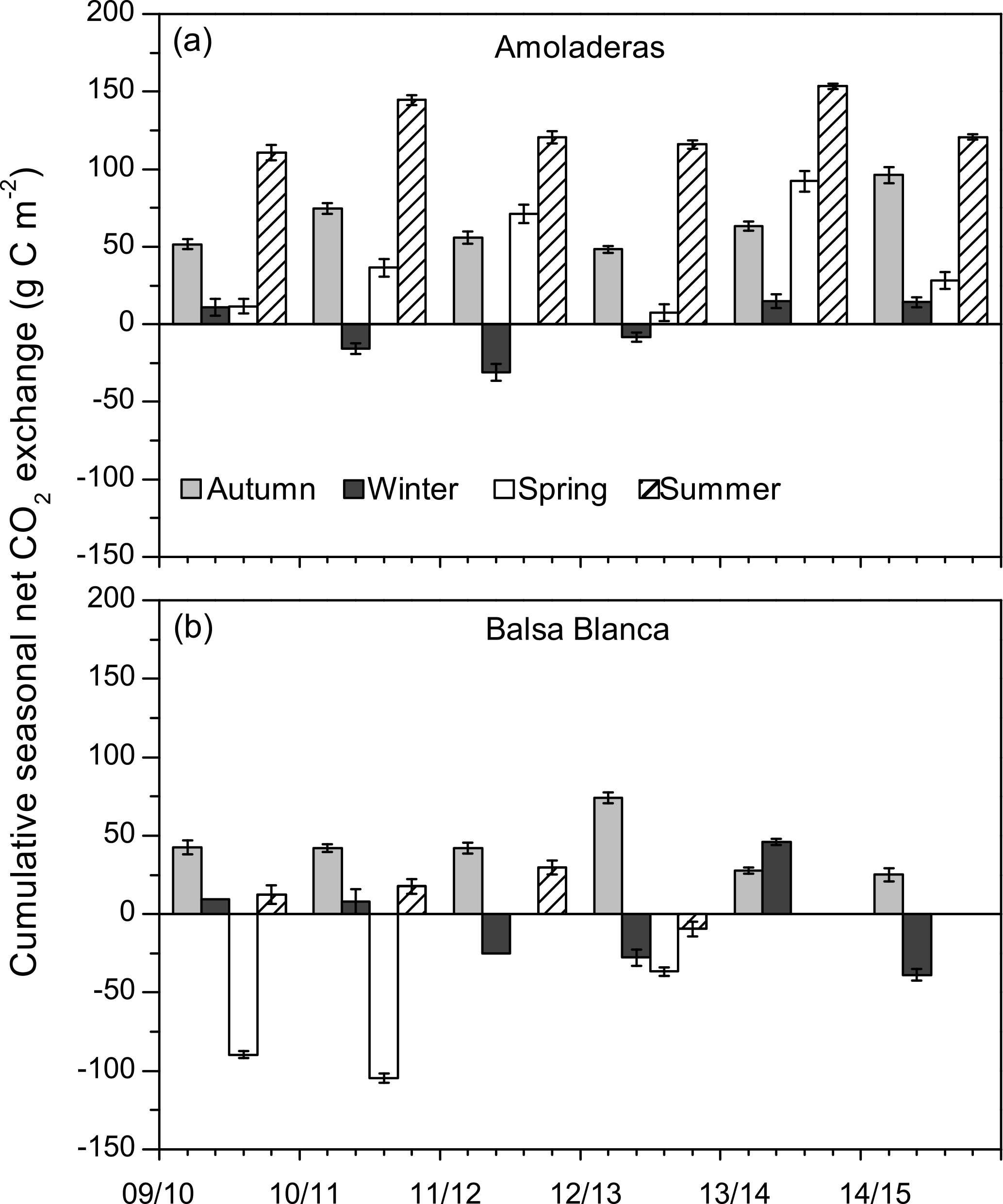
Figure 4Cumulative seasonal net CO2 exchange over the study period in both experimental sites. Negative values denote net carbon uptake, while positive values denote net carbon release. In the case of Balsa Blanca, missing bars correspond to long-term data losses (> 50 % data).
Overall, a positive and saturating trend was observed at both sites during autumn months until December–February when cumulative net CO2 releases started to decline. The autumn net CO2 release (i.e., positive values) was usually higher in AMO than in BB, except for 2012–2013, and the declining slope was always higher in BB, meaning greater net C uptake rates. Although the pattern of the cumulative net CO2 exchange showed differences between sites over autumn, winter and spring months, stronger discrepancies were found during summer droughts. From April–May to August, BB showed neutral behavior, while a remarkably positive trend was observed in AMO, denoting a large net CO2 release.
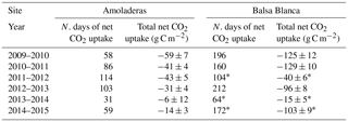
Table 4Number of days with daily net CO2 uptake and the related total C absorbed for every hydrological year and every field site of the study. Asterisks denote those years with abundant data losses (∼ 30 % data).
3.3 Seasonal and diurnal net CO2 exchanges
Long-term data loss occurred in BB during the springs of 2011–2012, 2013–2014 and 2014–2015 and summers of 2013–2014 and 2014–2015, when annual C balances could not be estimated. However, by observing the available seasonal data, it is noticeable that maximum and minimum seasonal net CO2 exchanges were very different between sites (Fig. 4). On one hand, maximum seasonal net CO2 uptake was measured during winter (December–February) in AMO and over spring (March–May) in BB, when peak net CO2 uptake equated to −31 g C m−2 (winter 2011–2012) and −105 g C m−2 (spring 2010–2011) in AMO and BB, respectively. Additionally, net CO2 uptake was only observed during three winters in the case of AMO, whereas it was frequently measured during both winter and spring in BB. On the other hand, the cumulative net CO2 release into the atmosphere occurred over all seasons in AMO but acutely in summer, when maximum seasonal net CO2 release was always observed ranging from 111 to 153 g C m−2. In contrast, in BB, the highest CO2 effluxes usually occurred in autumn ranging from 25 to 74 g C m−2, although significant CO2 release was also observed in winter 2013–2014 and the summers of 2009–2010 and 2011–2012. Regarding seasonal evapotranspiration (ET) fluxes, results showed a ∼ 30 % higher ET at BB compared to AMO during spring. Major intersite differences in autumn occurred in the first and last years of study, when ETs were 23 and 12 % higher at BB (Fig. 5).
When comparing daily-scale net CO2 exchange and ET fluxes with enhanced vegetation index (EVI) data, we notice some similarities in the general patterns of both sites (Fig. 6). There was a common annual pattern in which the highest values of EVI coincided with maximum net CO2 uptake rates (i.e., negative net CO2 fluxes), which in turn, corresponded to peak ET fluxes. Additionally, a decreasing trend in EVI over the 6 years of study was also noticeable for both sites. However, some intersite and interannual differences were evident (Fig. 6).
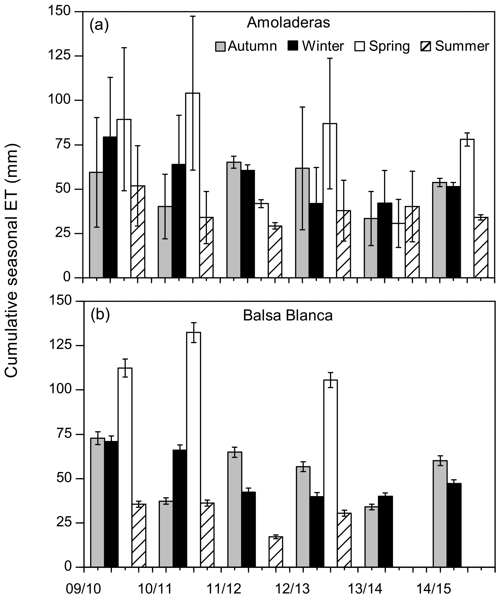
Figure 5Cumulative seasonal evapotranspiration fluxes (ET) over the study period at both experimental sites. In the case of Balsa Blanca, missing bars correspond to long-term data losses (> 50 % data). Error bars denote uncertainty derived from the gap-filling procedure.
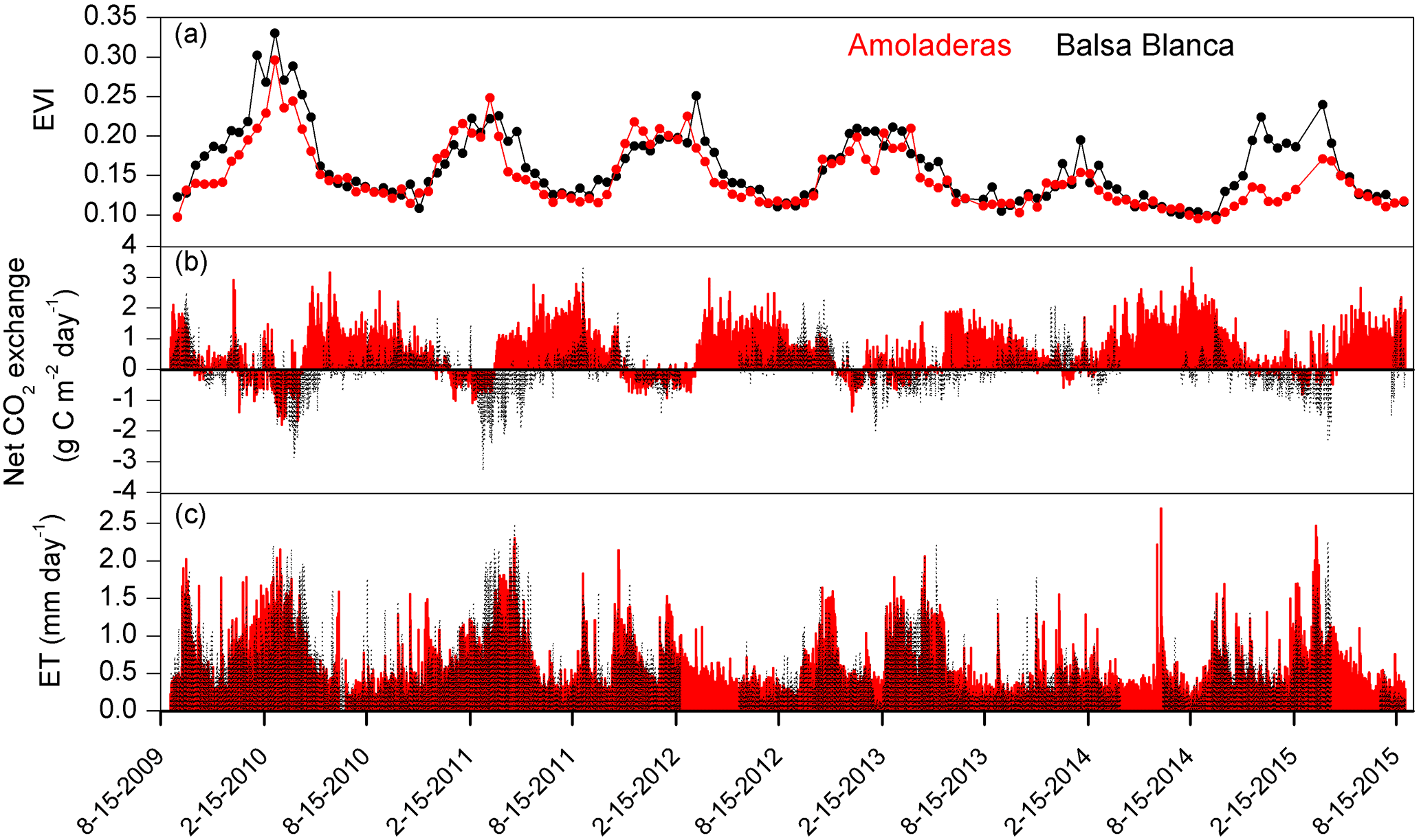
Figure 6Time series of (a) enhanced vegetation index (EVI), (b) daily net CO2 exchange and (c) daily evapotranspiration fluxes measured in Amoladeras (red lines and dots) and Balsa Blanca (black lines and dots) over 6 hydrological years (2009–2015). Long-term data losses correspond to periods of several months when ET and CO2 fluxes are absent.
On one hand, there were two main differences between sites. Firstly, extreme net CO2 release was measured uniquely in AMO during summer months (June–August), when maximum net CO2 fluxes ranging from 31 to 68 g C m−2 were measured (Fig. 6b). Over the study period, the monthly net CO2 exchange of AMO during dry seasons was up to 100 times higher than in BB (in August 2013), since monthly net CO2 fluxes measured in BB were much lower, from −8 to 16 g C m−2 (Fig. 6b). Besides the striking differences in summer net CO2 exchange between sites, minor discrepancies were also found in ET fluxes and EVI for the same drought periods. In this regard, monthly averaged ET over the dry season equated to 13 ± 4 and 10 ± 4 mm for AMO and BB, respectively, and EVI was on average 4 % higher in BB than in AMO (Fig. 6a and c). The second intersite difference was the greater net CO2 uptake over longer periods measured in BB. In particular, the period during which the ecosystems acted as C sinks lasted on average 38 days longer in BB than in AMO annually (Table 4). Accordingly, the annual amount of C fixation ranged from 6–59 g C m−2 at AMO and 15–129 g C m−2 at BB, with the annual averaged net C uptake in BB 162 % higher than at AMO (Table 4). Consequently, peak EVI values were usually observed during March–April for both sites; however, over winter and spring months (growing period), EVI measured at BB was 3–37 % higher than AMO, with the largest intersite differences in 2009–2010 and 2014–2015 (Fig. 6a). Likewise, monthly averaged ET fluxes measured at BB over winter and spring months (December–May) were from 3 to 24 % larger than those measured at AMO. Additionally, the growing period of the driest year (2013–2014) corresponded to the lowest monthly ET fluxes and the least difference between sites.
On the other hand, differences in the interannual variability of EVI were found between years. To be precise, 2009–2010 and 2013–2014 were the years with maximum and minimum annual precipitation and EVI observations, respectively, for both sites. In 2009–2010, EVI observations were 28 and 20 % higher than the 6-year averaged values in BB and AMO. In the driest year, 2013–2014, growing season (winter–spring) EVI was reduced to 35 and 28 %. Nevertheless, the largest difference between sites in winter–spring EVI observations was found in 2014–2015, following the driest year, when BB showed a pattern very similar to those registered over the years prior to the dry spell, while AMO still presented EVI values 21 % below the 6-year average (Fig. 6a).
3.4 Biological net CO2 exchange, gross primary production, ecosystem respiration and water use efficiency
The results of the “biological” annual C balance were obtained for AMO by applying the ventilation model and are in accordance with our hypotheses. Annual C emission was always measured at AMO, whereas BB acted as a neutral and mild C sink. On average, AMO emitted 32 g C m−2 more than BB. On a monthly timescale, net CO2 fluxes during autumn were, on average, ∼ 4 times higher at BB, except in the last study year, when the net CO2 emission at AMO was 21 times greater than at the natural site. However, during winter and spring months, net CO2 uptake was generally higher at the BB (Fig. 7a).
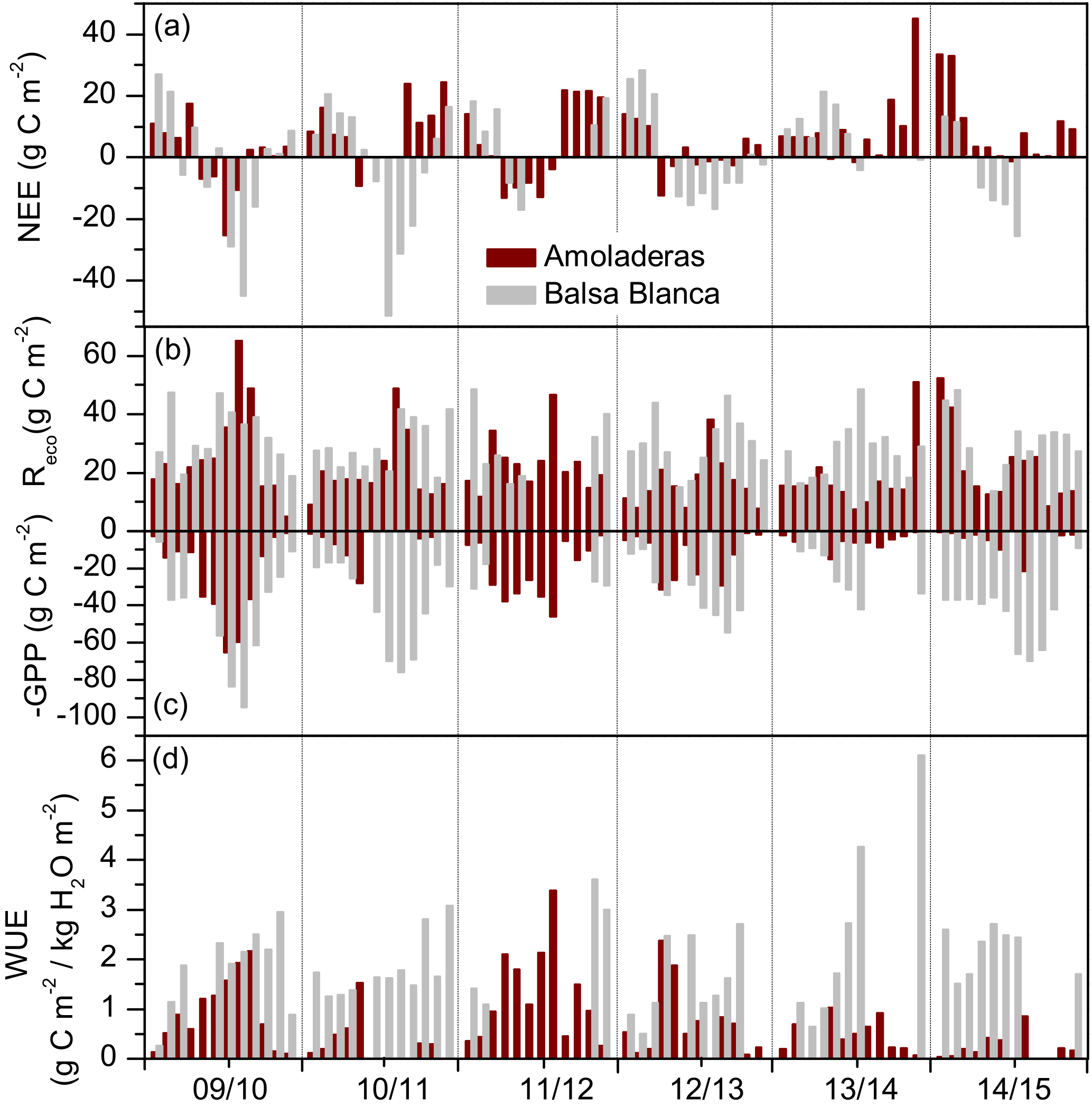
Figure 7Monthly cumulative fluxes of (a) biological net ecosystem CO2 exchange, (b) ecosystem respiration (Reco), (c) negative gross primary production and (d) water use efficiency over the 6 hydrological years of study (2009–2015) for Amoladeras (dark red) and Balsa Blanca (grey). Missing bars correspond to long-term data losses.
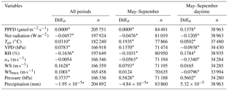
Table 5Results of the two-sided Wilcoxon summed rank test used to assess differences among meteorological variables measured at each experimental site over all periods, from May to September and from May to September during daytime, separately. Medians of the difference between the samples (Amoladeras minus Balsa Blanca) in standardized terms (Diffst) and number of observations are detailed. Significant results (p-value < 0.05) are denoted with asterisks, and bold values represent those variables with Diffst between sites above 1.
On average, during the 6 years of study, GPP, Reco and water use efficiency (WUE) were 9, 2 and 10 times higher at BB compared to AMO. Firstly, GPP was always higher at BB compared to AMO (Fig. 7c). Major differences occurred in autumn 2014–2015, when monthly cumulative GPP at BB was 32 times higher on average. Similarly, Reco was generally higher, up to ∼ 8 times at BB (October 2014). However, respiratory fluxes were occasionally greater at AMO, from 2 to 31 % higher, during spring and winter months of all studied years except 2013–2014 (Fig. 7b). Maximum intersite differences in GPP and Reco were found in winter and autumn 2014–2015, following the driest year, when monthly GPP was ∼ 30 times higher at BB compared to AMO. Similarly, monthly Reco was ∼ 5 times greater at BB. Intersite differences in partitioned fluxes could not be assessed during spring months due to the lack of data from BB. Secondly, WUE was lower at AMO during the entire study period, when maximum and minimum differences coincided with the highest and lowest differences in GPP between sites. On average, monthly WUE was 6 and 1.5 times higher at BB during winter and spring. Major intersite differences were found in autumn and winter 2014–2015 (Fig. 7d).
3.5 Differences in meteorological and soil variables between sites
Results from the two-sided Wilcoxon summed rank test (Table 5) showed significant differences (p-value < 0.05) between sites in most of the monitored meteorological variables. The few exceptions were the friction velocity (u*) when using the entire study period, the maximum wind speed registered every half-hour (WSmax) when analyzing May–September data, and the wind speed (WS) and precipitation when assessing daytime May–September data (Table 5). The large number of observations (n ranged from 21 410 to 205 751) produced highly significant results (Table 5). Hence, the standardized difference between the samples (Diffst) allowed us to quantitatively explore the differences between sites. Relevant differences (Diffst > 1) were found only for the subsoil CO2 molar fraction measured at 1.50 m depth (CO2,1.50 m) for all periods, and during May–September months even when using only daytime data (Table 6). In particular, CO2,1.50 m was always higher in AMO, from 889 to 1109 ppm (Tables S1–S3). Additionally, volumetric water content at 0.05 m depth (VWC0.05 m) was also higher in AMO compared to BB but only during summer months (Table 6), when absolute differences were very small, ranging from 0.028 to 0.037 m3 m−3 (Tables S1–S3). In contrast, subsoil CO2 molar fraction measured at 0.05 m depth (CO2,0.05 m) was from 89 to 150 ppm higher in BB when analyzing dry season (May–September) daytime data (Tables 6 and S1–S3).
Table 6Results of the two-sided Wilcoxon summed rank test used to assess differences among soil variables measured at each experimental site over all periods, from May to September and from May to September during daytime, separately. Medians of the difference between the samples (Amoladeras minus Balsa Blanca) in standardized terms (Diffst) and number of observations are detailed. Significant results (p-value < 0.05) are denoted with asterisks, and bold values represent those variables with Diffst between sites above 1.
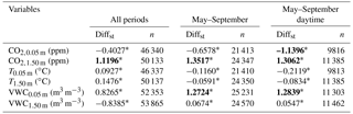
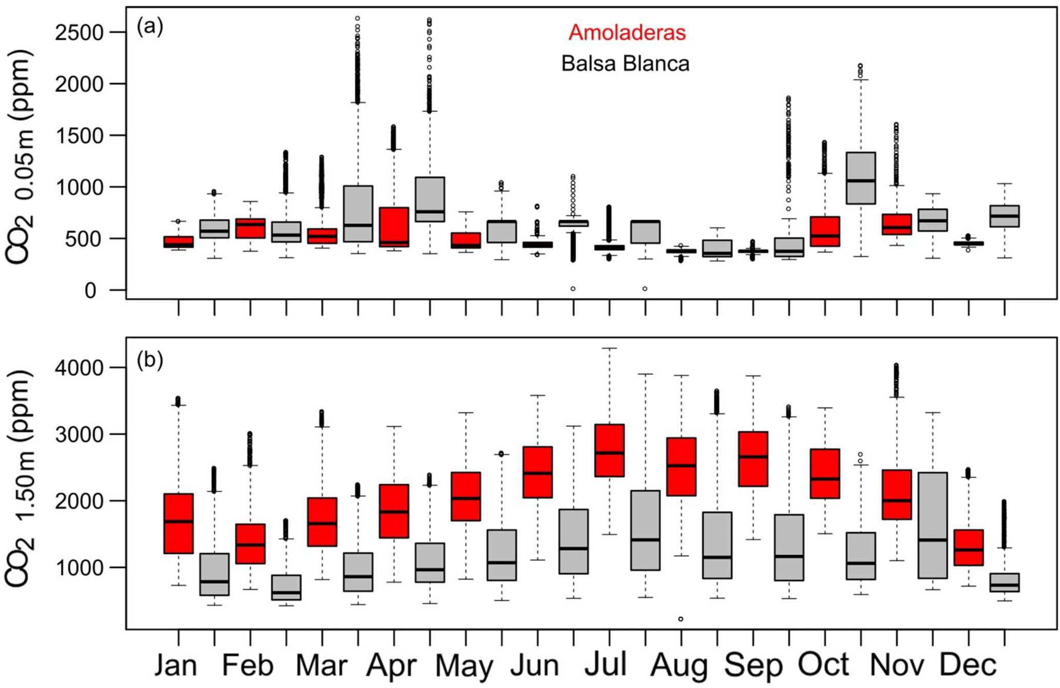
Figure 8Box-and-whisker plots of CO2 molar fractions measured at (a) 0.05 m and (b) 1.50 m belowground in Amoladeras (red boxes) and Balsa Blanca (grey boxes) from January 2014 to August 2015. The box extends from the first (Q1) to the third quartiles (Q3) and the central line represents the median (50 % percentile). Dots represent outliers; the upper whisker is located at the smaller of the maximum value and Q3 + 1.5 IQR (interquartile range), and the lower whisker is located at the larger of the minimum value and Q1 − 1.5 IQR.
The temporal dynamics of subsoil CO2 molar fractions revealed similar annual patterns between sites; generally, however, CO2,0.05 m was higher in BB, from 6 to 88 %, while CO2,1.50 m was always greater in AMO, from 31 to 97 % (Fig. 8). On one hand, the maximum monthly averaged values of CO2,0.05 m were registered in autumn, particularly in November and October which had 642 and 1120 ppm in AMO and BB, whereas minimum values occurred in September and August with 373 and 400 ppm at each site (Fig. 8a). On the other hand, peak monthly averaged values of CO2,1.50 m occurred in July for both sites, with 2751 and 1602 ppm in AMO and BB, although relatively high CO2,1.50 m was also measured during November in BB. In contrast, minimum values were observed in December and February, with 1364 and 735 ppm in AMO and BB, respectively (Fig. 8b).
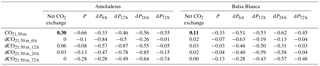
Finally, results of the Spearman correlation analysis between net CO2 exchange and belowground CO2 at 1.50 m depth (CO2,1.50 m) showed a positive relationship between both absolute variables, which was stronger for AMO compared to BB with Spearman correlation coefficients (rs) of 0.30 and 0.11, respectively (Table 7). In contrast, a negative relationship was found between pressure and CO2,1.50 m with higher rs in AMO compared to BB (Table 7). Additionally, rs were maxima at 12 h intervals for CO2,1.50 m and pressure increments (dP12 h) at AMO, and at 6 h intervals for CO2,1.50 m and pressure increments (dP6 h) at BB, with rs equal to −0.87 and −0.63.
Our results verify that land degradation affects the C sequestration capacity of semiarid ecosystems, since relevant differences between sites were observed during the growing season, when greater net C uptake over longer periods was observed at the natural site (BB). However, contrary to what we previously hypothesized, a much greater net C release was measured at the degraded site (AMO) over drought periods due to the predominance of subterranean ventilation (López-Ballesteros et al., 2017). In fact, the great difference in annual C budgets between sites (Fig. 3) was largely related to this process resulting in an average release of 196 ± 40 and −23 ± 20 g C m−2 yr−1 for the degraded and natural sites, respectively. Even when assessing only the biological net CO2 exchange, by subtracting the nonbiological CO2 flux when feasible, the degraded site emitted 32 g C m−2 more than the natural site. In this regard, the ecosystems' functioning could be divided into three different phases. The first phase corresponded to the autumn months, when the first rainfall events after the dry summer (i.e., rain pulses) activated the soil microbiota, triggering respiratory CO2 emissions as previously measured at the same experimental sites (López-Ballesteros et al., 2016; Rey et al., 2017). During this phase, maximum net CO2 emission was observed at the natural site, which exceeded the biological net CO2 flux observed at the degraded site (Fig. 7a). In fact, as hypothesized, Reco was generally higher at the natural site during autumn months (Fig. 7b), probably due to the greater pool of organic carbon (Table 1) and the potential differences in microbial communities (Rey et al., 2017) between sites. The second phase comprised the growing period when plants photosynthesized and also respired along with microorganisms under milder temperatures and better hydric conditions. During this phase, larger net CO2 uptake was measured at the natural site, with 162 % more than at the degraded site (Table 4) due to the higher vegetation cover and more fertile soils (Table 1) of the natural site. Accordingly, GPP estimates were, on average, 9 times higher at the natural site (Fig. 7c) and moreover, these results were supported by the lower ET, WUE and EVI values obtained in the degraded site during winter and spring months over the entire study period (Figs. 5, 6 and 7d). The third phase consisted of the dormancy period when water scarcity and high temperatures constrained biological activity. During this period, a neutral C balance was observed at the natural site, while extreme CO2 release was measured at the degraded site, as expected (Figs. 4 and 6b), where ventilative fluxes were dominant.
In order to detect potential factors driving the observed differences in the C balances, we checked whether soil and meteorological variables differed between sites. Our results demonstrated that some factors typically influencing GPP, Reco, and hence net ecosystem CO2 exchange, such as photosynthetic photon flux density (PPFD; Michaelis and Menten, 1913), precipitation (Berner et al., 2017; Jongen et al., 2011), vapor pressure deficit (VPD; Lasslop et al., 2010) and soil and air temperature (Lloyd and Taylor, 1994), did not differ between sites (Tables 5 and 6). Conversely, some differences were found for shallow soil volumetric water content (VWC0.05 m) during dry seasons (Table 6), when VWC0.05 m was 2 times higher in AMO than in BB, but absolute differences were slight, from 0.028 to 0.037 m3 m−3 (Tables S1–S3). Hence, although the important influence of soil moisture in both GPP and Reco is known (Tang and Baldocchi, 2005), we believe that differences in VWC0.05 m are not enough relevant to cause the differing ecosystem functioning observed over the drought period. Additionally, we think that this intersite difference in VWC0.05 m could be instrumental or due to the spatial variability of VWC0.05 m derived from the heterogeneity of soil morphological characteristics, since we only used one sensor at each site. Similarly, significant differences were not detected in several variables linked to subterranean ventilation, such as the friction velocity (u*; Kowalski et al., 2008), wind speed (WS; Rey et al., 2012a), half-hourly maximum wind speed (WSmax) and net radiation, which has been positively correlated to ventilative CO2 fluxes (López-Ballesteros et al., 2017), when using the analysis periods in which this process is supposed to be relevant, namely daytime hours during the dry seasons (Table 5). However, although no turbulence and wind speed intersite differences were found, interconnectivity of soil pores and fractures is probably higher at the degraded site (Table 1) due to its higher gravel and rock fractions (Table 1), which could lead to an enhanced penetration of eddies within the vadose zone (Pérez-Priego et al., 2013).
Table 7Spearman correlation coefficients (rs) for every paired simple correlation among maximum quality net CO2 exchange fluxes (µmol m−2 s−1), absolute and differential pressure (hPa) at 6, 12, 24 and 72 h time step and absolute and differential CO2 molar fraction measured at 1.50 m below ground (ppm) at the same time steps. Bold values represent the highest correlation coefficients, while shaded ones denotes nonsignificant relationships (p-values > 0.05).
Apart from that, outstanding differences between sites were observed in subsoil CO2 molar fractions measured at 0.05 and 1.50 m depths (CO2,0.05 m and CO2,1.50 m, respectively; Table 6). On one hand, CO2,0.05 m was generally higher at the natural site given its lower degradation level, which probably promotes higher root respiration and microbial activity supported by higher vegetation density and soil fertility (Table 1), especially during spring (Fig. 8), as also pointed out by Oyonarte et al. (2012). On the other hand, CO2,1.50 m values were acutely higher at the degraded site, by up to 1000 ppm compared to the natural site (Tables S1–S3). Therefore, we suggest that CO2,1.50 m is the main factor responsible for the intersite differences in net CO2 fluxes over the dry season. In this regard, previous research has suggested two potential origins of this vadose zone CO2: geological degassing (Rey et al., 2012b) and/or subterranean translocation of CO2 in both gaseous and aqueous phases (López-Ballesteros et al., 2017). However, not only does the amount of subsoil CO2 matter but also how effective its transport is, since both determine the net CO2 release from the vadose zone to the atmosphere. In this context, Oyonarte et al. (2012) found, in the same study area (Cabo de Gata-Níjar Natural Park), that soils with degradation symptoms, such as lower SOC, depleted biological activity, coarser texture and worse structure, showed higher soil CO2 effluxes over the dry season. Additionally, soil CO2 effluxes measured during summer months correlated positively with the fraction of rock outcrops, suggesting that deteriorated soil physical conditions actually enhanced vertical transfer of CO2-rich air from the subsoil to the atmosphere (Oyonarte et al., 2012). In fact, correlation analysis between CO2,1.50 m and net CO2 exchange/atmospheric pressure (Table 7) showed a stronger relationship between these variables at the degraded site. In this sense, ecosystem degradation could provoke a greater exposure of subsoil CO2 to the pressure effect, as described by Sánchez-Cañete et al. (2013), probably due to a higher fraction of bare soil, coarser structure, differing porosity type and/or thinner soil depth (Table 1).
Regarding EVI data, we found a discrepancy between GPP estimates and EVI values since, contrary to what is observed in EVI results, we observed that GPP was always higher at the natural site compared to the degraded site. We think that this is due to the different spatial scales defining each measurement. MODIS pixels have an area of ∼ 6.25 ha, while the eddy covariance footprint corresponds to a smaller area of ∼ 1 ha. Therefore, there is an EVI uncertainty that stems from the influence of other surface elements apart from vegetation, such as bare soil or outcrops within the pixel, which is our case. In fact, previous studies confirm the discrepancy between MODIS- and EC-derived GPP estimates, especially on sparse vegetation areas with low productivity (Gilabert et al., 2015). However, EVI data have allowed us to complement our findings based on CO2 fluxes, especially when EC data losses occurred. For instance, the declining trend observed from 2009–2010 to the end of the study period, for both sites, was not noticeable from EC data alone (Fig. 6). This long-term decrease in EVI may be related to a gradual drying following the wettest year (2009–2010), when extraordinarily high precipitation occurred (twice the mean annual precipitation for both sites over the study period). This EVI pattern also suggests a pulse-like behavior of ecosystem vegetation over the interannual timescale.
Moreover, in addition to demonstrating that degradation can influence the biological activity of ecosystems' vegetation, EVI results also showed that the degradation level can modulate how an ecosystem responds to a short-term disturbance. A clear example is the dry spell experienced in 2013–2014, when a reduction in EVI was measured during the growing season at both sites, i.e., 35 and 28 % at the natural and degraded sites, respectively. However, a year later (2014–2015), EVI values below the 6-year average were observed only at the degraded site (21 % lower; Fig. 6a) and major intersite differences were found for GPP, Reco and WUE during autumn and winter months (Fig. 7b–d). Accordingly, the natural site seemed to be more resilient than the degraded site against the short-term disturbance, since the effect of drought persisted in AMO even during the following year, while BB recovered to a pre-perturbation state within the same period (Fig. 6a). As a result, ecosystem resilience (Holling, 1973) was weakened by long-term disturbances such as land degradation, making degraded ecosystems more vulnerable to climate extremes (Reichstein et al., 2013). In this sense, mitigation policies to confront land degradation should be focused on prevention programs since ecosystem restoration does not recover complete ecosystem functionality (Lal, 2001; Moreno-Mateos et al., 2017). Moreover, even after several decades, relict degradation legacies can remain (Alados et al., 2011).
The present study can be seen as a step forward to better understanding the effect of land degradation on the intricate network of multiscale processes, factors and structures that define ecosystems' biological productivity and ultimately control their C balances. Despite some limitations, such as long-term data gaps, this research demonstrates that continuous ecosystem-scale EC observations remain crucial to comprehending how climate and land use change can modify the C sequestration capacity of ecosystems. In fact, annual average net CO2 exchanges of 196 ± 40 (C release) and −23 ± 20 g C m−2 yr−1 (C fixation) for the degraded and natural (i.e., site of reference) sites were measured, respectively. Additionally, larger net CO2 uptake over longer periods was observed at the natural site, with 162 % higher C compared to the degraded site, whereas a much greater net CO2 release was measured at the degraded site during drought periods. Accordingly, the estimates of gross primary production, ecosystem respiration and water use efficiency were, on average, 9, 2 and 10 times higher at the natural site. Future research should be based on the continuity of long-term monitoring stations, such as eddy covariance stations, in order to calibrate and validate satellite data, reduce uncertainties in the relationships between ecosystem productivity, land degradation and climate change and, finally, to improve the predictive ability of current terrestrial C models.
The eddy covariance data are available in the European Fluxes Database Cluster (http://www.europe-fluxdata.eu) where experimental sites have the codes Es-Amo and Es-Agu. Other data can be obtained by contacting the corresponding author.
The supplement related to this article is available online at: https://doi.org/10.5194/bg-15-263-2018-supplement.
FD, CO, AK and PSO designed the experiment. ALB, PSO, EPSC and MRM calibrated the sensors, collected the data and maintained the field instrumentation. EPSC designed subsoil data acquisition system and MRM processed subsoil data. ALB processed the eddy covariance data, made the figures and tables and wrote the manuscript. All authors reviewed the manuscript.
The authors declare that they have no conflict of interest.
This article is part of the special issue “Ecosystem processes and functioning across current and future dryness gradients in arid and semi-arid lands”. It is not associated with a conference.
Ana López-Ballesteros acknowledges support from the Spanish Ministry of
Economy and Competitiveness (FPI grant, BES-2012-054835). This work was
supported in part by the Spanish Ministry of Economy and Competitiveness
projects ICOS-SPAIN (AIC10-A-000474), SOILPROF (CGL2011-15276-E), GEI-Spain
(CGL2014-52838-C2-1-R), including European Union ERDF funds; and by the
European Commission project DIESEL (PEOPLE-2013-IOF-625988). We also thank
L. Morillas, O. Uclés and E. Arnau for field work.
Edited by: Tianshan Zha
Reviewed by: two anonymous referees
Ahlström, A., Raupach, M. R., Schurgers, G., Smith, B., Arneth, A., Jung, M., Reichstein, M., Canadell, J. G., Friedlingstein, P., Jain, A. K., Kato, E., Poulter, B., Sitch, S., Stocker, B. D., Viovy, N., Wang, Y. P., Wiltshire, A., Zaehle, S., and Zeng, N.: The dominant role of semi-arid ecosystems in the trend and variability of the land CO2 sink, Science, 348, 895–899, https://doi.org/10.1126/science.aaa1668, 2015.
Alados, C. L., Pueyo, Y., Barrantes, O., Escós, J., Giner, L., and Robles, A.: Variations in landscape patterns and vegetation cover between 1957 and 1994 in a semiarid Mediterranean ecosystem, Landsc. Ecol., 19, 543–559, 2004.
Alados, C. L., Puigdefábregas, J., and Martínez-Fernández, J.: Ecological and socio-economical thresholds of land and plant-community degradation in semi-arid Mediterranean areas of southeastern Spain, J. Arid Environ., 75, 1368–1376, 2011.
Bajocco, S., De Angelis, A., and Salvati, L.: A satellite-based green index as a proxy for vegetation cover quality in a Mediterranean region, Ecol. Indicat., 23, 578–587, 2012.
Baldocchi, D. D., Hincks, B. B., and Meyers, T. P.: Measuring biosphere–atmosphere exchanges of biologically related gases with micrometeorological methods, Ecology, 69, 1331–1340, 1988.
Berner, L. T., Law, B. E., and Hudiburg, T. W.: Water availability limits tree productivity, carbon stocks, and carbon residence time in mature forests across the western US, Biogeosciences, 14, 365–378, https://doi.org/10.5194/bg-14-365-2017, 2017.
Bown, H. E., Fuentes, J.-P., Perez-Quezada, J. F., and Franck, N.: Soil respiration across a disturbance gradient in sclerophyllous ecosystems in Central Chile, Ciencia e Investigación Agraria, 41, 89–106, 2014.
Cook, B. I., Smerdon, J. E., Seager, R., and Coats, S.: Global warming and 21st century drying, Clim. Dynam., 43, 2607–2627, https://doi.org/10.1007/s00382-014-2075-y, 2014.
del Barrio, G., Puigdefabregas, J., Sanjuan, M. E., Stellmes, M., and Ruiz, A.: Assessment and monitoring of land condition in the Iberian Peninsula, 1989–2000, Remote Sens. Environ., 114, 1817–1832, https://doi.org/10.1016/j.rse.2010.03.009, 2010.
Evans, S. E. and Wallenstein, M. D.: Climate change alters ecological strategies of soil bacteria, Ecol. Lett., 17, 155–164, https://doi.org/10.1111/ele.12206, 2014.
Feng, S. and Fu, Q.: Expansion of global drylands under a warming climate, Atmos. Chem. Phys., 13, 10081–10094, https://doi.org/10.5194/acp-13-10081-2013, 2013.
Feng, Q., Liu, W., Yanwu, Z., Jianhua, S., Yonghong, S., Zun Qiang, C., and Haiyang, X.: Effect of climatic changes and human activity on soil carbon in desertified regions of China, Tellus B, 58, 117–128, 2006.
Fensholt, R., Rasmussen, K., Kaspersen, P., Huber, S., Horion, S., and Swinnen, E.: Assessing land degradation/recovery in the African Sahel from long-term earth observation based primary productivity and precipitation relationships, Remote Sensing, 5, 664–686, 2013.
Gao, X. and Giorgi, F.: Increased aridity in the Mediterranean region under greenhouse gas forcing estimated from high resolution simulations with a regional climate model, Global Planet. Change, 62, 195–209, https://doi.org/10.1016/j.gloplacha.2008.02.002, 2008.
Gilabert, M. A., Moreno, A., Maselli, F., Martínez, B., Chiesi, M., Sánchez-Ruiz, S., García-Haro, F. J., Pérez-Hoyos, A., Campos-Taberner, M., Pérez-Priego, O., Serrano-Ortiz, P., and Carrara, A.: Daily GPP estimates in Mediterranean ecosystems by combining remote sensing and meteorological data, ISPRS J. Photogram. Remote Sens., 102, 184–197, https://doi.org/10.1016/j.isprsjprs.2015.01.017, 2015.
Grove, A. T. and Rackham, O.: The Nature of Mediterranean Europe. An Ecological History, Yale University Press, New Haven, London, 2001.
Holling, C. S.: Resilience and Stability of Ecological Systems, Annu. Rev. Ecol. System., 4, 1–23, 1973.
Hou, X., Wang, Z., Michael, S. P., Ji, L., and Yun, X.: The response of grassland productivity, soil carbon content and soil respiration rates to different grazing regimes in a desert steppe in northern China, Rangeland J., 36, 573–582, 2014.
Jongen, M., Pereira, J. S., Aires, L. M. I., and Pio, C. A.: The effects of drought and timing of precipitation on the inter-annual variation in ecosystem–atmosphere exchange in a Mediterranean grassland, Agr. Forest Meteorol., 151, 595–606, 2011.
Kottek, M., Grieser, J., Beck, C., Rudolf, B., and Rubel, F.: World map of the Köppen–Geiger climate classification updated, Meteorol. Z., 15, 259–263, 2006.
Kowalski, A. S., Serrano-Ortiz, P., Janssens, I. A., Sánchez-Moral, S., Cuezva, S., Domingo, F., Were, A., and Alados-Arboledas, L.: Can flux tower research neglect geochemical CO2 exchange?, Agr. Forest Meteorol., 148, 1045–1054, 2008.
Lal, R.: Potential of Desertification Control to Sequester Carbon and Mitigate the Greenhouse Effect, Climatic Change, 51, 35–72, https://doi.org/10.1023/a:1017529816140, 2001.
Lasslop, G., Reichstein, M., Papale, D., Richardson, A. D., Arneth, A., Barr, A., Stoy, P., and Wohlfahrt, G.: Separation of net ecosystem exchange into assimilation and respiration using a light response curve approach: critical issues and global evaluation, Global Change Biol., 16, 187–208, https://doi.org/10.1111/j.1365-2486.2009.02041.x, 2010.
Lloyd, J. and Taylor, J.: On the temperature dependence of soil respiration, Funct. Ecol., 8, 315–323, 1994.
López-Ballesteros, A., Serrano-Ortiz, P., Sánchez-Cañete, E. P., Oyonarte, C., Kowalski, A. S., Pérez-Priego, Ó., and Domingo, F.: Enhancement of the net CO2 release of a semiarid grassland in SE Spain by rain pulses, J. Geophys. Res.-Biogeo., 121, 52–66, https://doi.org/10.1002/2015jg003091, 2016.
López-Ballesteros, A., Serrano-Ortiz, P., Kowalski, A. S., Sánchez-Cañete, E. P., Scott, R. L., and Domingo, F.: Subterranean ventilation of allochthonous CO2 governs net CO2 exchange in a semiarid Mediterranean grassland, Agr. Forest Meteorol., 234–235, 115–126, https://doi.org/10.1016/j.agrformet.2016.12.021, 2017.
Mainguet, M. and Da Silva, G.: Desertification and drylands development: what can be done?, Land Degrad. Dev., 9, 375–382, 1998.
Mauder, M. and Foken, T.: Documentation and instruction manual of the eddy covariance software package 324 TK3, Abt. Mikrometeorol., 46, 28–36, 2004.
Mbow, C., Brandt, M., Ouedraogo, I., de Leeuw, J., and Marshall, M.: What four decades of earth observation tell us about land degradation in the Sahel?, Remote Sensing, 7, 4048–4067, 2015.
Michaelis, L. and Menten, M. L.: Die Kinetik der Invertinwirkung, Biochem. Z., 49, 333–369, 1913.
Moncrieff, J. B., Massheder, J. M., de Bruin, H., Elbers, J., Friborg, T., Heusinkveld, B., Kabat, P., Scott, S., Soegaard, H., and Verhoef, A.: A system to measure surface fluxes of momentum, sensible heat, water vapour and carbon dioxide, J. Hydrol., 188–189, 589–611, https://doi.org/10.1016/S0022-1694(96)03194-0, 1997.
Moreno-Mateos, D., Barbier, E. B., Jones, P. C., Jones, H. P., Aronson, J., López-López, J. A., McCrackin, M. L., Meli, P., Montoya, D., and Rey Benayas, J. M.: Anthropogenic ecosystem disturbance and the recovery debt, Nat. Commun., 8, 14163, https://doi.org/10.1038/ncomms14163, 2017.
Niemeijer, D., Puigdefabregas, J., White, R., Lal, R., Winslow, M., Ziedler, J., Prince, S., Archer, E., King, C.: Dryland Systems, in: Ecosystems and Human Well-being: Current State and Trends, in: Vol. 1, Millennium Ecosystem Assessment Series, Island Press, Washington, USA, 623–662, 2005.
Omuto, C.: A new approach for using time-series remote-sensing images to detect changes in vegetation cover and composition in drylands: A case study of eastern Kenya, Int. J. Remote Sens., 32, 6025–6045, 2011.
Omuto, C., Vargas, R., Alim, M., and Paron, P.: Mixed-effects modelling of time series NDVI-rainfall relationship for detecting human-induced loss of vegetation cover in drylands, J. Arid Environ., 74, 1552–1563, 2010.
Oyonarte, C., Rey, A., Raimundo, J., Miralles, I., and Escribano, P.: The use of soil respiration as an ecological indicator in arid ecosystems of the SE of Spain: Spatial variability and controlling factors, Ecol. Indicat., 14, 40–49, https://doi.org/10.1016/j.ecolind.2011.08.013, 2012.
Pérez-Priego, O., Serrano-Ortiz, P., Sánchez-Cañete, E. P., Domingo, F., and Kowalski, A. S.: Isolating the effect of subterranean ventilation on CO2 emissions from drylands to the atmosphere, Agr. Forest Meteorol., 180, 194–202, 2013.
Poulter, B., Frank, D., Ciais, P., Myneni, R. B., Andela, N., Bi, J., Broquet, G., Canadell, J. G., Chevallier, F., Liu, Y. Y., Running, S. W., Sitch, S., and Van Der Werf, G. R.: Contribution of semi-arid ecosystems to interannual variability of the global carbon cycle, Nature, 509, 600–603, https://doi.org/10.1038/nature13376, 2014.
Prince, S., Becker-Reshef, I., and Rishmawi, K.: Detection and mapping of long-term land degradation using local net production scaling: Application to Zimbabwe, Remote Sens. Environ., 113, 1046–1057, 2009.
Pugnaire, F. I., Haase, P., Incoll, L. D., and Clark, S. C.: Response of the tussock grass Stipa tenacissima to watering in a semi-arid environment, Funct. Ecol., 10, 265–274, 1996.
Puigdefábregas, J. and Mendizabal, T.: Perspectives on desertification: western Mediterranean, J. Arid Environ., 39, 209–224, 1998.
Puigdefabregas, J. and Mendizabal, T.: Prospects of desertification impacts in western Europe, in: Environmental Challenges in the Mediterranean 2000–2050, NATO Science Series, IV. Earth and environmental Sciences, edited by: Marquina, A., Springer, Dordrecht, p. 155, 2004.
Reichstein, M., Falge, E., Baldocchi, D., Papale, D., Aubinet, M., Berbigier, P., Bernhofer, C., Buchmann, N., Gilmanov, T., Granier, A., Grünwald, T., Havránková, K., Ilvesniemi, H., Janous, D., Knohl, A., Laurila, T., Lohila, A., Loustau, D., Matteucci, G., Meyers, T., Miglietta, F., Ourcival, J.-M., Pumpanen, J., Rambal, S., Rotenberg, E., Sanz, M., Tenhunen, J., Seufert, G., Vaccari, F., Vesala, T., Yakir, D., and Valentini, R.: On the separation of net ecosystem exchange into assimilation and ecosystem respiration: review and improved algorithm, Global Change Biol., 11, 1424–1439, https://doi.org/10.1111/j.1365-2486.2005.001002.x, 2005.
Reichstein, M., Bahn, M., Ciais, P., Frank, D., Mahecha, M. D., Seneviratne, S. I., Zscheischler, J., Beer, C., Buchmann, N., Frank, D. C., Papale, D., Rammig, A., Smith, P., Thonicke, K., Van Der Velde, M., Vicca, S., Walz, A., and Wattenbach, M.: Climate extremes and the carbon cycle, Nature, 500, 287–295, https://doi.org/10.1038/nature12350, 2013.
Rey, A., Pegoraro, E., Oyonarte, C., Were, A., Escribano, P., and Raimundo, J.: Impact of land degradation on soil respiration in a steppe (Stipa tenacissima L.) semi-arid ecosystem in the SE of Spain, Soil Biol. Biochem., 43, 393–403, 2011.
Rey, A., Belelli-Marchesini, L., Were, A., Serrano-ortiz, P., Etiope, G., Papale, D., Domingo, F., and Pegoraro, E.: Wind as a main driver of the net ecosystem carbon balance of a semiarid Mediterranean steppe in the South East of Spain, Global Change Biol., 18, 539–554, https://doi.org/10.1111/j.1365-2486.2011.02534.x, 2012a.
Rey, A., Etiope, G., Belelli-Marchesini, L., Papale, D., and Valentini, R.: Geologic carbon sources may confound ecosystem carbon balance estimates: Evidence from a semiarid steppe in the southeast of Spain, J. Geophys. Res., 117, G03034, https://doi.org/10.1029/2012JG001991, 2012b.
Rey, A., Oyonarte, C., Morán-López, T., Raimundo, J., and Pegoraro, E.: Changes in soil moisture predict soil carbon losses upon rewetting in a perennial semiarid steppe in SE Spain, Geoderma, 287, 135–146, https://doi.org/10.1016/j.geoderma.2016.06.025, 2017.
Rodríguez-Fernández, L. R., López-Olmedo, F., Oliveira, J. T., Medialdea, T., Terrinha, P., Matas, J., Martín-Serrano, A., Martín-Parra, L. M., Rubio, F., Marín, C., Montes, M. and Nozal, F.: Mapa geológico de la Península Ibérica, Baleares y Canarias a escala 1/1.000.000, Instituto Geológico y Minero de España (IGME), National Institute of Geography of Spain – IGME, http://mapas.igme.es/Servicios/default.aspx#IGME_Geologico_1M (last access: December 2017), 2015.
Sánchez-Cañete, E. P., Kowalski, A. S., Serrano-Ortiz, P., Pérez-Priego, O., and Domingo, F.: Deep CO2 soil inhalation/exhalation induced by synoptic pressure changes and atmospheric tides in a carbonated semiarid steppe, Biogeosciences, 10, 6591–6600, https://doi.org/10.5194/bg-10-6591-2013, 2013.
Schulz, K., Voigt, K., Beusch, C., Almeida-Cortez, J. S., Kowarik, I., Walz, A., and Cierjacks, A.: Grazing deteriorates the soil carbon stocks of Caatinga forest ecosystems in Brazil, Forest Ecol. Manage., 367, 62–70, 2016.
Serrano-Ortiz, P., Oyonarte, C., Pérez-Priego, O., Reverter, B., Sánchez-Cañete, E. P., Were, A., Uclés, O., Morillas, L., and Domingo, F.: Ecological functioning in grass–shrub Mediterranean ecosystems measured by eddy covariance, Oecologia, 175, 1005–1017, https://doi.org/10.1007/s00442-014-2948-0, 2014.
Shoshany, M, and Karnibad, L.: Remote Sensing of Shrubland Drying in the South-East Mediterranean, 1995–2010: Water-Use-Efficiency-Based Mapping of Biomass Change, Remote Sensing, 7, 2283–2301, 2015.
Tang, J. and Baldocchi, D. D.: Spatial–temporal variation in soil respiration in an oak–grass savanna ecosystem in California and its partitioning into autotrophic and heterotrophic components, Biogeochemistry, 73, 183–207, 2005.
Thompson, M., Vlok, J., Rouget, M., Hoffman, M., Balmford, A., and Cowling, R.: Mapping grazing-induced degradation in a semi-arid environment: a rapid and cost effective approach for assessment and monitoring, Environ. Manage., 43, 585–596, 2009.
Uclés, O., Villagarcía, L., Moro, M. J., Canton, Y., and Domingo, F.: Role of dewfall in the water balance of a semiarid coastal steppe ecosystem, Hydrol. Process., 28, 2271–2280, https://doi.org/10.1002/hyp.9780, 2014.
UNCCD – United Nations Convention to Combat Desertification: General Assembly, A/AC.241/27, http://www.unccd.int/Lists/SiteDocumentLibrary/conventionText/conv-eng.pdf (last access: December 2016), 1994.
Wang, W., Guo, J., and Oikawa, T.: Contribution of root to soil respiration and carbon balance in disturbed and undisturbed grassland communities, northeast China, J. Biosci., 32, 375–384, 2007.
Watanabe, M. D. B. and Ortega, E.: Ecosystem services and biogeochemical cycles on a global scale: valuation of water, carbon and nitrogen processes, Environ. Sci. Policy, 14, 594–604, https://doi.org/10.1016/j.envsci.2011.05.013, 2011.