2.1 Study area

Gwangyang Bay is a semi-enclosed bay system, located on the southern coast of the Korean Peninsula, and is one of the most industrialized coastal areas exposed to anthropogenic pressure. It starts from Seomjin River and goes through Yeosu Channel (between Yeosu Peninsula and Namhae Island) to the open ocean (the East China Sea). The bay area covers approximately 145 km², and water depth is generally shallow at 2.4–8.0 m in the northern upper-middle Seomjin River estuarine channel compared with 10–30 m in the deep-bay channel (Kim et al., 2014). The annual freshwater discharges of Seomjin River are 10.7–39.3 × 10⁸ tons. The seasonality of nutrient input from the catchment area (ca. 5 × 10³ km²), including agricultural and forested land, is profound (Kwon et al., 2002). The wet season starts from late spring and the discharge peaks during the summer monsoon period.

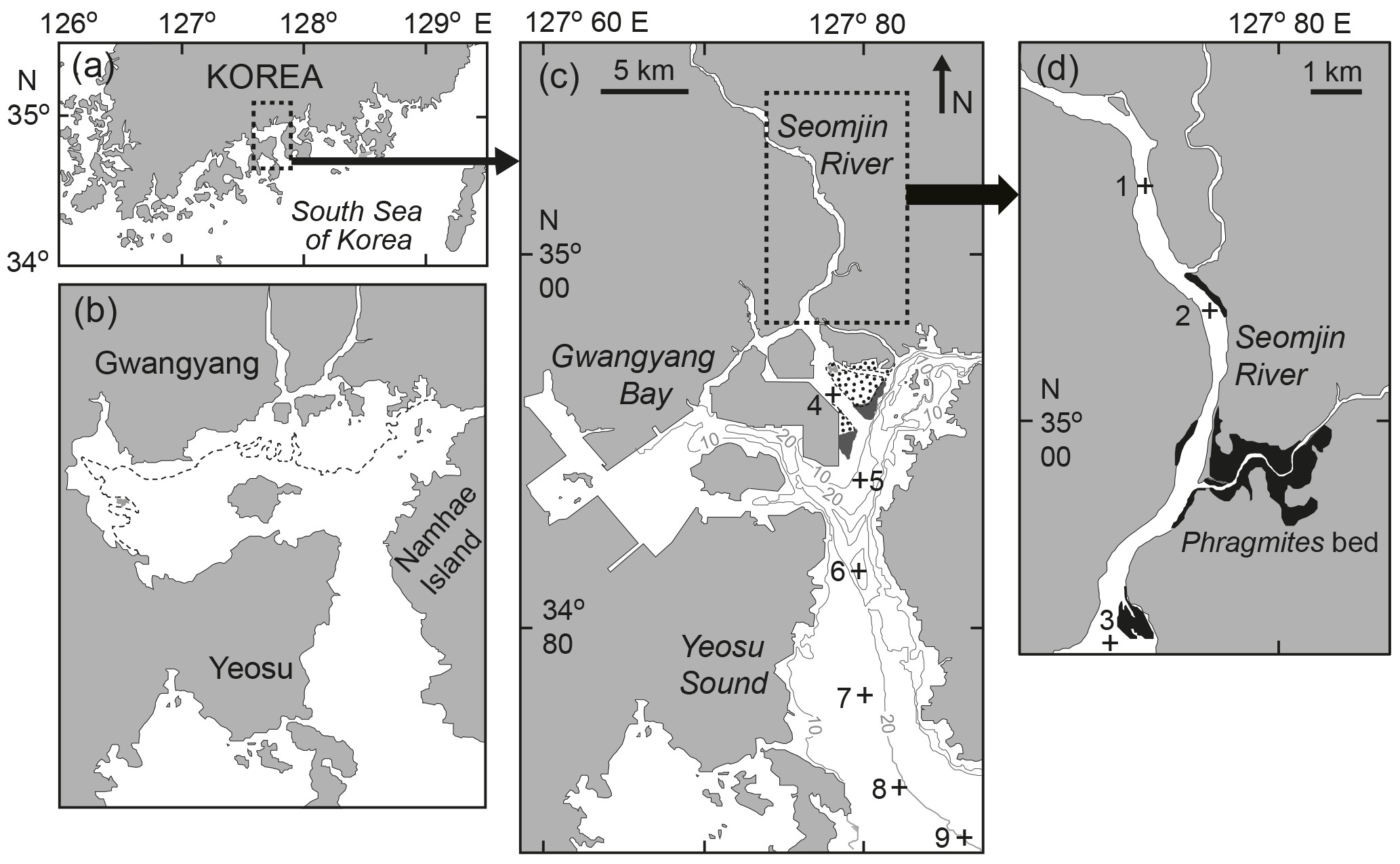
Figure 1Map showing the location of Gwangyang Bay (a), the appearance of the bay before the reclamation of tidal flats in 1982 (b), and the sampling stations in the bay (c) and in the estuarine channel (d). The broken line represents the lowest water line (b); the dotted areas show intertidal beds and the dark gray areas Zostera beds (c); and the darker areas show Phragmites beds (d).

Download

Accordingly, the maximum median river discharge varies from 30–95 m³ s⁻¹ in the dry season to 300–400 m³ s⁻¹ in the summer monsoon, with an annual mean of ca. 120 m³ s⁻¹ (Kim et al., 2014). The tidal cycle of the bay is semidiurnal with maximum ranges of 3.40 m during spring tides and 1.10 m during neap tides. Tidal currents from the Yeosu Channel also strongly influence the system, and approximately 82 % of the Seomjin River flux is discharged toward this channel. Overall, increasing industrial pollution facilitates eutrophic conditions in the estuarine and related bay waters. Diatoms dominate in the phytoplankton community, and density is high in the middle part of Gwangyang Bay (Kim et al., 2009; data from our parallel study not shown). The distribution patterns of copepods in the Seomjin River during summer were represented by three main salinity zones: an oligohaline zone (dominated by Pseudodiaptomas koreanus, Sinocalanus tenellus, and Tortanus dextrilobatus), a mesohaline zone (dominated by Acartia ohtsukai and Acartia forticrusa), and a polyhaline zone (dominated by Acartia erythraea, Calanus sinicus, Centropages dorsispinatus, Labidocera rotunda, and Paracalanus parvus) (Park et al., 2015).

2.2 Sampling and processing

Surface water and net-tow samples were collected seasonally (February, May, August, and November) at nine stations from the head to the mouth of Gwangyang Bay in 2015 (Fig. 1). The stations were chosen based on salinity regime and different geographic characteristics. Stations 1–3 were located in the Seomjin River, stations 4 and 5 were in Gwangyang Bay (the middle part of the estuary), and stations 6–9 were located from the offshore deep-bay channel to the southern mouth of the estuary. On each sampling occasion, water temperature and salinity were determined in situ using an YSI Model 85 probe (YSI Inc., Yellow Springs, OH, USA).

Zooplankton taxonomic samples were collected during daytime by net towing using a plankton net (45 cm diameter, 200 µm mesh size) equipped with a flowmeter (Model 2030R Mechanical Flowmeter, General Oceanics Inc., Miami, FL) and gently hauled horizontally at a subsurface depth of 0.5–1 m with the ship speed at about 1 knot (0.5 m s⁻¹). The average volume filtered per tow was 16.7 ± 5.1 m³ (mean ± se). Samples were fixed in formalin solution with a final concentration of 5 % and then identified and enumerated under a stereomicroscope (SMZ 645; Nikon, Tokyo, Japan) in the laboratory. At each station, one additional net tow was collected for isotope analysis. After collection, specimens were transferred immediately into plastic bottles and preserved in a refrigerator (4 ^∘C) until analysis. In the laboratory, subsamples were picked out from the mixed zooplankton samples under a dissecting microscope. Easily distinguishable zooplankton groups such as harpacticoids were separated from a mixture of calanoids and cyclopoids. Copepodites were counted but grouped together with adults. All subsamples were lyophilized and then homogenized by pulverizing them with a mortar and pestle before isotope analysis.

POM in surface water (0.5–1 m depth) was collected using a 5 L Niskin bottle at a midday high tide at the same time as zooplankton collection. The approximately 20 L seawater collected was first screened through a 200 µm Nitex mesh to remove zooplankton and large-sized particles. The prescreened water samples were transported to the laboratory as soon as possible within 1–2 h. In the laboratory, water samples were filtered again through a 20 µm Nitex mesh and then filtered onto precombusted (450 ^∘C for 4 h) Whatman GF/F glass fiber filters to determine isotope ratios of fine POM (< 20 µm) representing pico- and nano-sized plankton. To obtain enough plankton cells for isotope analysis of coarse POM (≥ 20 µm), we collected POM samples by net towing with a plankton net of 50 cm diameter and 20 µm mesh size. After collection, each sample was prefiltered through a 200 µm Nitex mesh to remove large particles and zooplankton. Both size fractions of samples were prepared in duplicate. Samples for δ¹³C measurements were acidified by fuming for about 5 h over concentrated HCl in a vacuum desiccator to remove carbonates, while the samples for δ¹⁵N measurements were not acidified. All the samples were lyophilized and pulverized with a mortar and pestle before isotope analysis.

For chlorophyll a (Chl a) determination, 1 L subsamples of surface water were filtered through Waterman GF/F glass fiber filters. The filters for Chl a (including other photosynthetic pigments) were extracted with 95 % methanol (5 mL) for 12 h in the dark at −20 ^∘C and sonicated for 5 min to foster cell disruption. Aliquots of 1 mL of the supernatants were mixed with 300 µL of water; 100 µL of this solution was analyzed by reverse-phase high-performance liquid chromatography (HPLC, LC-20A HPLC system, Shimadzu Co., Kyoto, Japan) using a Water Symmetry C₈ (4.6 × 150 mm, particle size: 3.5 µm, 100 Å pore size) column (Waters, Milford, MA, USA) and a method derived from Zapata et al. (2000). Quantification of standard pigments was calculated by a spectrophotometer with the known specific extinction coefficients after Jeffrey (1997). Sample peaks were identified based on their retention time compared with those of pure standards. Further details on analysis, calibration, and quantification have been given elsewhere (Lee et al., 2011; Kwak et al., 2017).

2.3 Isotope analysis

For measurements of carbon and nitrogen stable isotope ratios, all pretreated samples were analyzed using a continuous-flow isotope ratio mass spectrometer (CF-IRMS; Isoprime100, Cheadle, UK) connected to an elemental analyzer (vario Micro cube, Hanau, Germany) following the procedure described by Park et al. (2016). Briefly, powdered samples were sealed in tin combustion cups and filter samples were wrapped with a tin plate. All prepared samples were put into the elemental analyzer to oxidize at high temperature (1030 ^∘C). CO₂ and N₂ gases were introduced into the CF-IRMS with the carrier being helium gas. Data of isotope values are shown in terms of δX, indicating the relative differences between isotope ratios of the sample and conventional standard reference materials (Vienna Pee Dee Belemnite for carbon, and atmospheric N₂ for nitrogen), which were calculated by the following equations: $\mathit{\delta }X=\left[\left(R_{\mathrm{sample}}/R_{\mathrm{standard}}\right)-\mathrm{1}\right]\times {\mathrm{10}}^{\mathrm{3}}$, where X is ¹³C or ¹⁵N and R_sample and R_standard are the ratios of heavy to light isotope for samples and standards, respectively. International standards of sucrose (ANU C₁₂H₂₂O₁₁; National Institute of Standards and Technology (NIST), Gaithersburg, MD, USA) for carbon and of ammonium sulfate ([NH₄]₂SO₄; NIST) for nitrogen were used for calibration after analyzing every 5–10 samples. The analytical precision for 20 replicates of urea were approximately ≤ 0.1 and ≤ 0.05 ‰ for δ¹³C and δ¹⁵N, respectively.

2.4 Data analysis

We used multiple linear regression to assign the isotopic value to each species from a mixture sample. As we did not measure the dry weights of each species directly, we calculated them using published empirical equations of the relationship between body length and dry weight of each species, and we searched the literature for the range of body length and their living environment of each species in the “World of Copepods Database” and related references (Table S1 in the Supplement). Those calanoid species primarily living in a marine environment based on the definition of the “World of Copepods Database” and related references were grouped as marine calanoids in this paper and included Acartia hudsonica, Acartia omorii, Bestiolina coreana, Calanus sinicus, Clausocalanus furcatus, Centropages abdominalis, Centropages dorsispinatus, Paracalanus aculeatus, Paraeuchaeta plana, Labidocera rotunda, Labidocera euchaeta, Tortanus dextrilobatus, and Tortanus forcipatus. The group of brackish calanoids included Acartia ohtsukai, Acartia erythraea, Eurytemora Pacifica, Paracalanus parvus, Pseudodiaptomus koreanus, Pseudodiaptomus marinus, and Sinocalanus tenellus.

Assuming that the proportion we picked to do isotope analysis was the same as the proportion in samples for composition analysis, once the weights of different groups or different genera/species were assigned, we computed the isotope ratio for each group by multiple linear regression models as in the following equations:

where m is the weight of the total community and m₁m_X are the weight of different groups or genera of each group. δ¹³C₁δ¹³C_X and δ¹⁵N₁δ¹⁵N_X are the δ¹³C and δ¹⁵N values of each group or genus, respectively. We used R software to do the estimation using the whole sampling data set. Insignificant results for sparse species, such as Bestiolina coreana, Clausocalanus furcatus, Paraeuchaeta plana, Oithona davisae, and Oncaea venella, found in Gwangyang Bay are not tested separately, while they were incorporated to respective groups based on their living environment.

Given that the isotopic values of consumers come from their diets and thereby from mixed proportions of different sources, the proportions of each source could be simulated by linear mixing models with a fractionation factor (also called a trophic enrichment factor). For instance, a mass balance mixing model is given by

where f₁−f_n are the proportion of different sources and α_Carbon and α_Nitrogen are trophic enrichment factors for δ¹³C and δ¹⁵N values, respectively.

Here, a Bayesian isotopic mixing model (available as an open source Stable Isotope Analysis package in R: SIAR) was performed to estimate the relative contribution of nanoplankton (defined by fine POM in the present study) and microplankton (coarse POM) to the copepod diets, as well as copepods to the carnivore diets (Parnell et al., 2010, 2013). The model assumes that each isotopic ratio of consumers follows the pattern of a Gaussian distribution with an unknown mean and standard deviation. The structure of mean values of consumers is a weighted combination of the food sources' isotopic values. The weights make up dietary proportions (given by a Dirichlet prior distribution). The standard deviation is divided up between the uncertainty around the fractionation corrections and the natural variability between all individuals within a defined group (Parnell et al., 2010, 2013). Because the values of consumers calculated from bulk copepod samples using the previous multiple linear regression models were only means and standard errors, we generated a vector consisting of 250 numbers for each group by a random normal distribution function. We then used the default iteration numbers (iterations = 500 000, burin = 50 000) provided by the SIAR package to perform our analysis. Fractionation factors used in the model estimation were estimated by difference of TLs multiplied by 3 ‰ per TL for δ¹⁵N and by 0.5 ‰ per TL for δ¹³C, respectively. TLs were calculated from the δ¹⁵N difference between consumer and source as follows (Post, 2002): (TL = $\mathrm{1}+({\mathit{\delta }}^{\mathrm{15}}{\mathrm{N}}_{\mathrm{consumer}}-{\mathit{\delta }}^{\mathrm{15}}{\mathrm{N}}_{\mathrm{source}})/\mathrm{3}$). Concentrations of isotope per mass among different diets (nanoplankton, microplankton, and major copepod genera) were not considered in this study. Model fitting was done via a Markov Chain Monte Carlo (MCMC) protocol that produces simulations of plausible values of the dietary proportions of each source. More details on model simulation can be found elsewhere (Parnell et al., 2010, 2013).

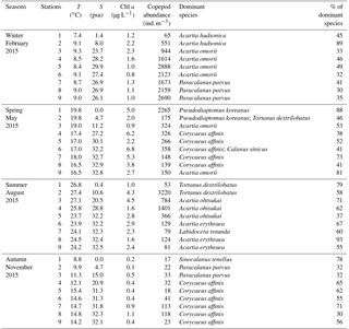
Table 1Seasonal variations in basic environmental factors, including temperature (T), salinity (S), and chlorophyll a (Chl a), copepod abundance, and dominant species and the percentage (%) of dominant species in total copepods at the nine stations in the Gwangyang Bay system.

Download Print Version | Download XLSX

All statistical analyses were performed using R 3.4.0 software (https://cran.r-project.org/bin/windows/base/). Regression analyses of copepod isotopic values were performed by generalized additive models (GAMs) using the mgcv library (Wood and Wood, 2015). Data were smoothed by cubic regression splines and fitted by the family of Gaussian functions. One-way analysis of variance (ANOVA) was adopted to test seasonal differences in environmental factors and copepod abundances, and Student's t tests were used to test for significant differences in mean δ¹³C and δ¹⁵N values between nano- and microplankton. Before applying ANOVA and t tests, the data were tested for normality of distribution and equal variance; significance was assumed at P=0.05. For the coefficients of variation, we calculated them by dividing the standard error with mean value.

3.1 Environmental variability and zooplankton abundances

Environmental factors including temperature, salinity, Chl a levels, copepod abundance, dominant species, and percentages of total copepods are shown in Table 1. Water temperature was significantly higher in summer and lower in winter (ANOVA, P < 0.001). The spatial variability in salinity was significant, with extremely low values at stations 1 and 2 (the river mouth), and then the values gradually increased to station 5 (the middle of the bay). Chl a concentrations ranged from 0.1 to 6.8 µg L⁻¹, and they were significantly higher in spring and summer than in winter and autumn (ANOVA, P < 0.01). The highest Chl a concentration occurred in the middle of the bay during the spring, while the lowest concentration was found at the river station during the autumn. The seasonal variability in copepod abundance was significant (ANOVA, P < 0.01), with higher abundances in winter when temperatures and Chl a concentrations were low.

Figure 2Temporal and spatial variations in plankton δ¹³C (‰) and δ¹⁵N (‰).

Download

The detailed abundance composition of copepods is shown in Table S2. Seasonal and spatial variations in dominant species (> 10 % of total abundance) of copepods were apparent (Table 1). The marine calanoid Acartia dominated at the river mouth to the middle part of the bay, while Paracalanus dominated at the mouth of the bay during winter. Acartia also dominated at the most highly saline stations in summer, except for station 7, where the community was dominated by Labidocera rotunda. A brackish water-preferring calanoid species, Pseudodiaptomus, dominated stations 1 and 2 at the river mouth in spring, and another brackish calanoid species, Sinocalanus, dominated station 1 in autumn. At the river mouth stations in summer, copepods were unexpectedly dominated by the marine calanoid species Tortanus dextrilobatus. The cyclopoid species Corycaeus affinis mainly dominated the most highly saline stations in spring and autumn.

3.2 Variability in plankton δ¹³C and δ¹⁵N values

The δ¹³C values of size-fractionated plankton (< 20 and 20–200 µm) and mixed copepod samples showed distinct spatial variations in each season (Fig. 2a–c). The δ¹³C values of nanoplankton (< 20 µm POM) ranged from −27.6 to −19.4 ‰, with a mean of −22.7 ‰ (Fig. 2a). The lowest δ¹³C value of nanoplankton was found at station 1 (the upper stream station of Seomjin River) in spring and the highest at station 9 (the mouth of the estuary) in summer. The δ¹³C values of microplankton (20–200 µm POM) ranged from −26.3 to −17.8 ‰, with a mean of −20.8 ‰ (Fig. 2b), being significantly higher than those of nanoplankton (paired t test, t=7.6, P < 0.001). Its lowest δ¹³C value was found at station 2 in spring and the highest at station 8 in winter. Overall, similar to nanoplankton, the microplankton δ¹³C values were more negative at the river portion (stations 1–3) and less negative at the mouth of the estuary (stations 7–9). The δ¹³C values of mixed copepods ranged from −25.9 to −16.4 ‰, with a mean of −20.1 ‰ (Fig. 2c). The lowest was found at station 1 in autumn and the highest at station 8 in summer. The spatial variability in copepod δ¹³C values followed the pattern of POM δ¹³C values. However, the copepod δ¹³C values were significantly higher than those of nanoplankton (paired t test, t=8.6, P < 0.001) and microplankton (t=3.1, P=0.004). Their δ¹³C values were higher in summer and winter than in spring and autumn. At stations 1–3, river input lowered the δ¹³C values of nanoplankton during the wet season (spring to summer). At stations 4–9, significantly lower δ¹³C values were observed in autumn than in other seasons (ANOVA, F=13.4, P < 0.001). For copepods, the autumn values were significantly lower than those in other seasons (ANOVA, F=5.9, P=0.004).

Table 2Coefficients (F) and significance levels (p) of the effects of variable predictors on δ¹⁵N of nanoplankton (plankton < 20 µm) and microplankton (plankton > 20 µm) using a generalized additive model test. P value < 0.05 indicates significance. The abbreviation “n.s.” stands for “no significance”.

Download Print Version | Download XLSX

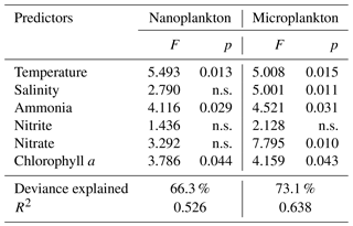
The δ¹⁵N values exhibited wider fluctuations than δ¹³C values (coefficients of variation = 29.3 % vs. 9.0 %, 21.5 % vs. 11.8 %, and 18.8 % vs. 13.1 % for nanoplankton, microplankton, and copepods, respectively). The δ¹⁵N values of nanoplankton ranged from 3.2 ‰ (station 4 in summer) to 8.8 ‰ (station 1 in winter), with a mean of 5.6 ‰ (Fig. 2d). There were distinct patterns in the three locations of the bay. The δ¹⁵N values tended to decline with distance from the river mouth, then increased in the middle of the bay, and decreased again toward the mouth of the estuary. The nanoplankton δ¹⁵N values were higher in winter than in other seasons (paired t test, t=5.4, P=0.001 for spring; t=3.0, P=0.017 for summer; t=4.1, P=0.004 for autumn). As indicated by regression analyses between the distribution of nanoplankton δ¹⁵N and environmental factors (Table 2), significant increases in the nanoplankton δ¹⁵N values depend on ammonia (GAM, F=4.1, P=0.029) and Chl a (GAM, F=3.8, P=0.044). In addition, the seasonal distribution of nanoplankton δ¹⁵N values was well indicated by their relationship with temperature among different seasons (GAM, $F=-\mathrm{5.5}$, P=0.013), with decreasing values in summer to autumn.

Mean δ¹⁵N value of microplankton (7.6 ‰), ranging from 4.8 ‰ (station 2 in spring) to 10.2 ‰ (station 6 in spring), was significantly higher than that of nanoplankton (paired t test, t=4.9, P < 0.001). The microplankton δ¹⁵N values were higher in summer than in other seasons (ANOVA, F=4.6, P=0.009), with the spatial trend vanishing in summer. Indeed, spatial trends differed between seasons, increasing progressively from the river mouth to the bay mouth in spring and autumn and decreasing in winter. As tested by GAM analysis, the microplankton δ¹⁵N values were elevated stepwise by environmental factors including temperature (GAM, F=5.0, P=0.015), salinity (GAM, F=5.0, P=0.031), ammonia (GAM, F=4.5, P=0.031), and nitrate (GAM, F=7.8, P=0.010). Similar to nanoplankton, regression analysis also showed that the microplankton δ¹⁵N values increased significantly with increasing Chl a concentrations (GAM, F=4.2, P=0.043).

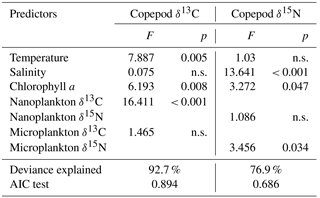
Copepod δ¹⁵N values ranged from 6.6 to 12.3 ‰ and were higher in summer than in other seasons (ANOVA, F=15.6, P < 0.001). Generalized additive model analysis showed that the deviances of copepod δ¹³C and δ¹⁵N values explained by the GAMs were 92.7 and 76.9 %, respectively (Table 3). Copepod δ¹³C values changed significantly toward increasing salinity (GAM, F=7.9, P=0.005), for both the nanoplankton (GAM, F=6.2, P=0.008) and the microplankton (GAM, F=16.4, P < 0.001; Fig. S1a–c in the Supplement). In contrast, temperature was the most important factor to explain the variability in copepod δ¹⁵N values (GAM, F=13.6, P < 0.001; Fig. S1d). The microplankton δ¹⁵N value was another important contributor to the variability in copepod δ¹⁵N values (GAM, F=3.5, P=0.034; Fig. S1e), while nanoplankton δ¹⁵N was not (GAM, P > 0.05). The Chl a concentration influenced the variability in copepod δ¹⁵N values significantly (GAM, F=3.3, P=0.047; Fig. S1f).

Figure 3Bi-plots of major plankton groups and genus isotopes in Gwangyang Bay.

Download

Table 3Coefficients (F) and significance levels (p) of the effects of variable predictors on δ¹³C and δ¹⁵N copepods using a generalized additive model test. P value < 0.05 indicates significance. The abbreviation “n.s.” stands for “no significance”.

Download Print Version | Download XLSX

3.3 Trophic positions of major groups

Multiple linear regression analyses to estimate mean isotopic values of different copepod groups (i.e., brackish calanoids, marine calanoids, and cyclopoids) from mixed copepod values (excluding harpacticoids) were all significant (R²=0.94, P < 0.001 for δ¹³C; R²=0.78, P < 0.001 for δ¹⁵N). The intercepts of the model indicating the errors of Eqs. (1) and (2) were 1.1 ± 0.8 and 0.3 ± 0.8 ‰ for δ¹³C and δ¹⁵N, respectively. The two calanoid groups displayed a close mean δ¹⁵N value (around 9 ‰) but significantly different δ¹³C values (−26.3 ± 1.5, −20.6 ± 1.6, and −20.1 ± 1.2 ‰ for brackish water calanoids and marine calanoids, respectively; Fig. 3a). Cyclopoids occupied a relatively broad trophic niche based on a big coefficient of variation (41.6 %), and the mean δ¹³C value of cyclopoids (−31.0 ± 6.0 ‰) was even lower than those of brackish calanoids. The δ¹⁵N values of the three major groups were all higher than the basal food resource (nanoplankton) and relatively higher than microplankton with some overlap of error bar. The values of harpacticoids isolated from the winter (stations 2–9) and spring samples (stations 1) were measured directly. The mean δ¹⁵N values of harpacticoids (6.9 ± 0.6 ‰) were lower than those of other copepods and microplankton, but the δ¹³C values (−16.7 ± 1.4 ‰) of Harpacticoids were relatively higher than other groups.

The multiple linear regression analysis performed for major copepod genera/species was also significant (R²=0.99, P < 0.001 for δ¹³C; R²=0.88, P < 0.001 for δ¹⁵N). The intercepts were 0.4 ± 0.7 and 0.8 ± 0.3 ‰ for δ¹³C and δ¹⁵N, respectively. There were two to three different trophic positions in the mixed copepod assemblages based on different δ¹⁵N values (see patterns in Fig. 3b). The mean δ¹⁵N values of Corycaeus affinis (13.7 ± 5.6 ‰) were the highest among the taxa, followed by those of Labidocera (12.3 ± 3.9 ‰), Tortanus (12.3 ± 1.9 ‰), Sinocalanus (11.3 ± 1.7 ‰), and Paracalanus (11.0 ± 3.6 ‰). The mean values of Acartia (9.4 ± 2.6 ‰), Calanus Sinicus (9.0 ± 1.1 ‰), Centropages (8.1 ± 1.7 ‰), and Eurytemora pacifica (7.4 ± 2.5 ‰) indicated their trophic positions were relatively lower than those carnivorous species, while they were higher than nanoplankton. Pseudodiaptomus had the lowest value of δ¹⁵N (5.3 ± 2.5 ‰), and it was even lower than microplankton and not much different to nanoplankton. Compared to of the two putative food resources (nanoplankton and microplankton), those brackish calanoid genera/species (Pseudodiaptomus, E. pacifica, Paracalanus and Sinocalanus) and Corycaeus had lower δ¹³C than nanoplankton, while marine calanoid genera/species (Tortanus, Labidocera, Calanus, Acartia and Centropages) had higher values (Fig. 3b).

The trophic level in this study was defined as trophic position relative to nanoplankton, which was considered as the trophic baseline. Considering that the TL of nanoplankton is 1, the TL value of microplankton was calculated to be 0.7 times higher than that of nanoplankton (Fig. 4). As a whole assemblage balanced from different feeding behaviors, as indicated by the standard errors, copepods occupied a 1.2 level higher TL than that of nanoplankton, indicating herbivory (here, herbivory means a trophic level of 2) on nanoplankton with slight omnivory (TL = 2–3) on other dietary sources. The TLs of two major calanoid groups (marine calanoids and brackish calanoids) were similar to the bulk copepod assemblage with mean levels slightly higher than 2. The mean TL value of cyclopoids apparently had a higher trophic level than calanoids. In contrast, the mean TL of harpacticoids was very low, reflected by their low δ¹⁵N values.

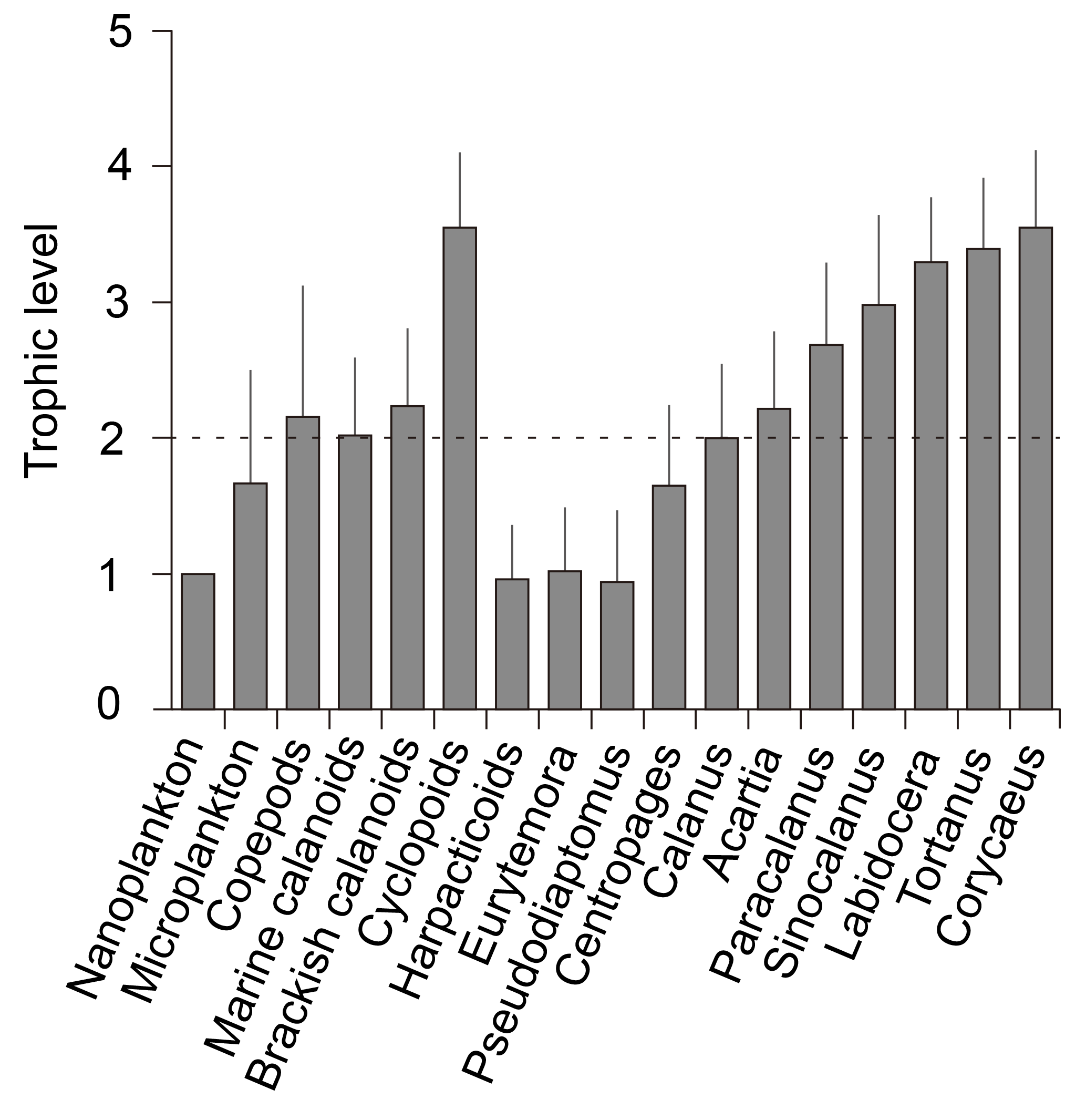
Figure 4Trophic levels (TLs) of different groups. Nanoplankton were set as TL = 1, while consumers' trophic levels were calculated as TL = $\mathrm{1}+({\mathit{\delta }}^{\mathrm{15}}{\mathrm{N}}_{\mathrm{consumer}}-{\mathit{\delta }}^{\mathrm{15}}{\mathrm{N}}_{\mathrm{Nanoplakton}})/\mathrm{3}$. The reference line indicates the herbivores relative to nanoplankton. However, nanoplankton here might not be truly primary producers as the bulk samples might include heterotrophic flagellates, dinoflagellates, and ciliates, which we could not separate from the collected samples.

Download

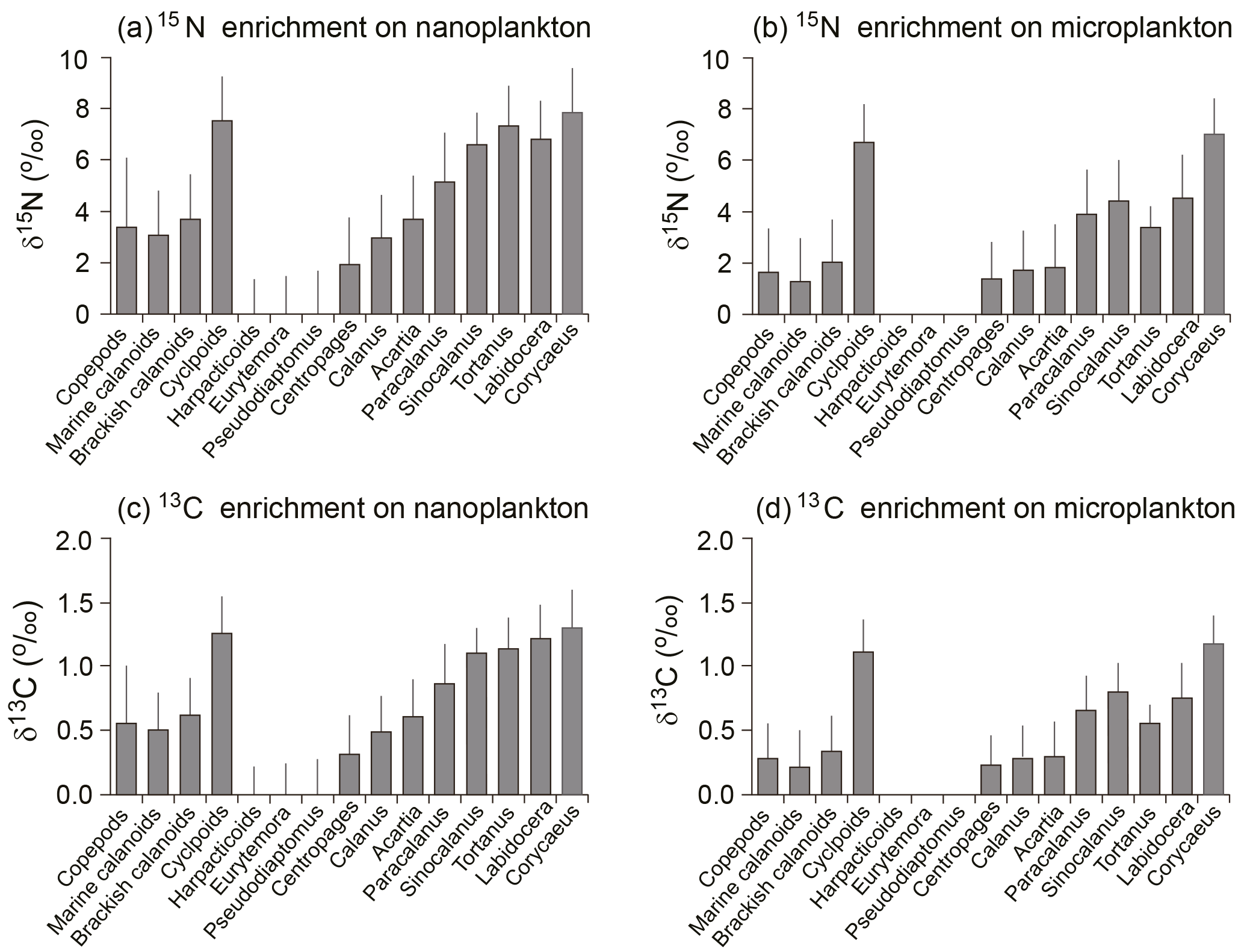
Figure 5Trophic enrichment (or fractionation factor) from basal food items (nanoplankton: a, c; microplankton: b, d), based on the difference of each sample's δ¹⁵N between higher trophic level and lower trophic level; a 0.5 ‰ per one trophic level was used to calculate the δ¹³C enrichment for each group. Reference lines indicate mean values from all groups.

Download

Among calanoids, the mean TLs of Eurytemora pacifica (1 ± 0.5) and Pseudodiaptomus (1 ± 0.5) are indicative of their herbivorous and/or detrivorous characteristics. The mean TLs of Calanus sinicus (2.0 ± 0.6) and Centropages (1.6 ± 0.6) indicated they were primarily herbivorous; and those of Acartia and Paracalanus were slightly higher than 2, indicating they were primarily omnivorous, feeding on both nanoplankton and microplankton. The levels of Sinocalanus (3.0 ± 0.7), Tortanus, and Labidocera were higher than 3.

Based on TLs, the mean ¹⁵N enrichments of the copepod assemblage were estimated to be 3.4 and 1.7 ‰ for nanoplankton and microplankton, respectively (Fig. 5a, b). The enrichment values on nanoplankton for both marine and brackish calanoids, as well as for the genera of Acartia, were close to the average value of the copepod assemblage. The trophic enrichment of Calanus sinicus on nanoplankton (3.0 ± 1.7 ‰) was slightly lower than averaged marine calanoids and total copepods, while the enrichment on microplankton (1.7 ± 1.5 ‰) was similar. Centropages (1.9 ± 1.8 ‰) had much lower enrichment on nanoplankton compared to total copepods and marine calanoids. Four high-TL genera Tortanus, Labidocera, Sinocalanus, and Corycaeus had high enrichments > 6 on nanoplankton and > 3 on microplankton.

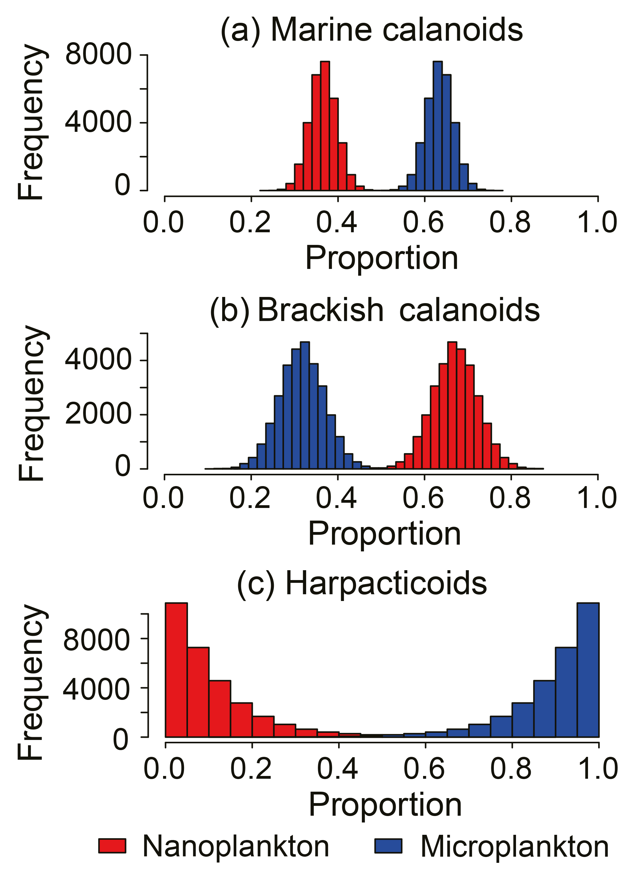
Figure 6Comparison of the dietary compositions of major copepod groups: (a) Marine calanoids, including Acartia hudsonica, Acartia omorii, Bestiolina coreana, Calanus sinicus, Clausocalanus furcatus, Centropages abdominalis, Centropages dorsispinatus, Paracalanus aculeatus, Paraeuchaeta plana, Labidocera rotunda, Labidocera euchaeta, Tortanus dextrilobatus, and Tortanus forcipatus; (b) brackish calanoids, including Acartia ohtsukai, Acartia erythraea, Eurytemora Pacifica, Paracalanus parvus, Pseudodiaptomus koreanus, Pseudodiaptomus marinus, and Sinocalanus tenellus; and (c) harpacticoids.

Download

Figure 7Comparison of the dietary compositions of the major omnivorous copepod genera.

Download

The ¹³C enrichments for total copepods were on average 0.6 and 0.3 ‰ when feeding on nanoplankton and microplankton, respectively (Fig. 5c, d). Patterns were same with enrichments on ¹⁵N. The four high-TL genera Tortanus, Labidocera, Sinocalanus, and Corycaeus had high enrichments > 1.2 on nanoplankton and > 0.6 on microplankton. The enrichments of four herbivorous/omnivorous species increased from Centropages, Calanus, and Acartia to Paracalanus. In contrast, the brackish calanoid genera Eurytemora and Pseudodiaptomus had extremely low enrichments of both ¹⁵N and ¹³C.

3.4 Contribution of size-fractionated POM to copepod diets

The Bayesian mixing model calculations showed that the contributions of different sizes of POM to copepod diets varied significantly with season (Student's t test, P < 0.001 for all cases; Fig. 7). Size-selective feeding phenomena were particularly apparent in winter (Fig. S2a) and summer (Fig. S2c). Mean contributions of microplankton accounted for about two-thirds of their assimilated diets at all stations in winter and summer and were almost equal to that of nanoplankton in spring and autumn (Fig. S2b, d). The proportions of the two size fractions of POM averaged from all four seasons contributing to copepod diets were also distinctly different at stations 2–5 and station 9 (Fig. S2). The mean contributions of microplankton to the copepod diets increased gradually from the river mouth up to a peak (0.81 ± 0.11) in the middle part of the bay. Then, the proportion declined gradually to a trough (0.31 ± 0.18) at the deep-bay channel. The proportion then rebounded to a high level again at the bay mouth station.

Figure 8Comparison of the dietary composition of major carnivorous genera. Credibility intervals of 95 % (dots), 75 % (whiskers), and 25 % (boxes) and mean values (lines in the boxes) are shown in box plots for each source.

Download

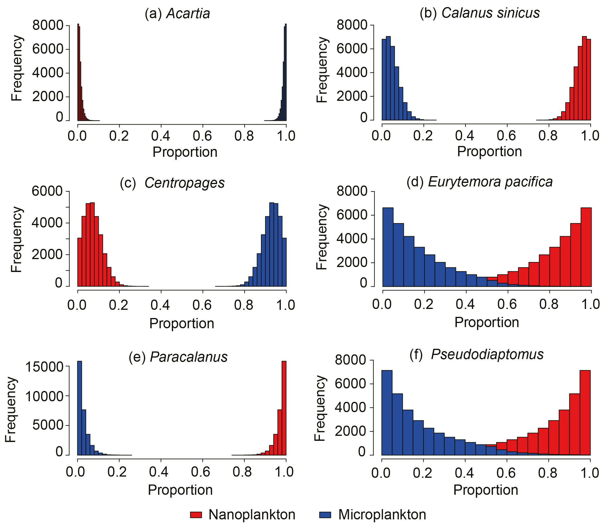
Three major groups of copepods showed contrasting size-selective feeding behaviors (Fig. 6). Marine calanoids typically preferred feeding on larger particles, with a contributing proportion of 0.63 ± 0.03 (range: 0.50–0.71) for microplankton (Fig. 6a). Harpacticoids had a more apparent size-selective feeding behavior, preferring microplankton (0.89 ± 0.10), and merely fed on nanoplankton (extremely low reliance of < 0.11; Fig. 6c). In contrast, brackish calanoids preferred feeding on nanoplankton (0.68 ± 0.05) to on microplankton (0.32 ± 0.05). For herbivorous/omnivorous copepod genera/species (e.g., Acartia, C. sinicus, Centropages, E. pacifica, Paracalanus, and Pseudodiaptomus), we tested their feeding preference on the two size fractions of POM using the Bayesian mixing model (Fig. 7). Acartia and Centropages significantly preferred large to small particles (Student's t test, P < 0.001) with a reliance of > 0.9 on microplankton (Fig. 7a, c); on the other hand, C. sinicus and Paracalanus apparently preferred small particles (Student's t test, P < 0.001) (Fig. 7b, e). The two “low trophic level” species/genera Eurytemora pacifica and Pseudodiaptomus selected nanoplankton more while there were large proportions of both potential food sources in diets (Fig. 7d, f). Based on the TL shown above, we considered that the four genera (Labidocera, Sinocalanus, Tortanus, and Corycaeus) are carnivorous and able to predate on other copepods. Thus, we tested the two fractions of POM and some herbivorous/omnivorous species/genera as potential food sources for them. The dietary compositions estimated by Bayesian mixing models showed a slight difference among them (Fig. 8). Except for Sinocalanus, the other three carnivorous species all showed only negligible reliance on the two size fractions of POM. The marine calanoid genus Labidocera preferred predating on Centropages (0.35 ± 0.08), followed by harpacticoids (0.15 ± 0.10), Acartia (0.13 ± 0.09), and Calanus (0.10 ± 0.07) (Fig. 8a). By contrast, besides feeding on nanoplankton (0.23 ± 0.03), the brackish calanoid genus Sinocalanus also preferred predating on other brackish calanoids Paracalanus (0.37 ± 0.02), Pseudodiaptomus (0.15 ± 0.03), and cyclopoids (0.09 ± 0.02) (Fig. 8b). Tortanus frequently co-occurred with many other copepods, and its diet was composed of many different copepod species/genera without apparent selectivity (Fig. 8c). The cyclopoid species Corycaeus affinis primarily predated on Paracalanus (0.67 ± 0.05) and Pseudodiaptomus (0.22 ± 0.06).

4.1 Variability in δ¹³C and δ¹⁵N values of plankton with time and space

We found that seasonal variations and the spatial heterogeneity of copepod δ¹³C and δ¹⁵N values in Gwangyang Bay followed those of nanoplankton (POM < 20 µm) and microplankton (POM > 20 µm) (Figs. 2 and 3). Based on the results of regression analyses, we found that the variability in copepod isotopic values was influenced by salinity (spatial variations), temperature (temporal variations), and isotopic values of food sources (both spatial and temporal variations; Fig. 3). In general, spatial variations were much more pronounced because of the effect of river input and thereby riverine carbon in different salinity regimes. More negative values of three plankton groups (nanoplankton, microplankton, and copepods) were measured near the river mouth, and then the values increased progressively to the mouth of the estuary, indicating an apparently decreasing effect of river runoff and thus the uptake of carbon derived from river-borne terrestrial organic matter. These results are consistent with other studies in estuarine environments (Cifuentes et al., 1988; Matson and Brinson, 1990; Thornton and McManus, 1994; Deegan and Garritt, 1997; Fry, 2002). Such spatial distribution patterns have also been found for other primary producers such as seagrasses (reviewed by Hemminga and Mateo, 1996), macroalgae (Lee, 2000), as well as benthic microalgae (Kang et al., 2003), and the pattern will further propagate to consumers such as fish (Melville and Connolly, 2003; Herzka, 2005), oysters (Fry, 2002), mollusks (Antonio et al., 2010), and other benthic macroinvertebrates (Choy et al., 2008).

Seasonal successions of δ¹³C values were also apparent, probably because of high river input in spring, elevated productivity in summer, and species successions in autumn. When the wet season started in spring and phytoplankton started to bloom, river input lowered the δ¹³C values. The values increased again in summer because of the persistence of phytoplankton bloom (a low fractionation effect because of source limitation) and elevated productivity in summer. Although both river discharge and the input of light carbon were low in autumn, the observed δ¹³C values were low. This was probably because of the lack of a heavy carbon pool (a dissolved inorganic carbon pool in which the carbon was primarily composed of heavy ¹³C) due to microbial respiration and species succession (Rau et al., 1990). During the post-bloom period in autumn, phytoplankton show low productivity and Chl a concentrations, with low abundance of diatoms but a dominance of flagellates (Baek et al., 2015). Flagellates are known to have more negative δ¹³C values than those of diatoms arising from different fractionation effects (Gearing et al., 1984; Cifuentes et al., 1988; Rolff, 2000).

The δ¹⁵N variability in the three major plankton groups was relatively complex spatially. The seasonal pattern of nanoplankton δ¹⁵N values, with decreasing values in summer to autumn, can be well explained by the relationship between the δ¹⁵N values and temperature, indicated by significant GAM analysis. Spatial trends in the nanoplankton δ¹⁵N values can be explained by three distinct distribution patterns. The first pattern found in the river mouth area exemplifies a declining trend expected from the mixing of freshwater planktonic materials, which grew up in water with high levels of dissolved inorganic nitrogen. The second pattern found in the middle part of the bay, in which nitrate inputs were low while the concentrations of ammonia increased (Kwon et al., 2004; our own data, not shown), characterizes an increase in δ¹⁵N values in association with high Chl a concentrations. Fractionations by autotrophic assimilation and bacterial utilization were the most likely source of the ¹⁵N-enriched ammonia in the nutrient pools of the middle of the bay (Cifuentes et al., 1988). The elevated POM δ¹⁵N values in the middle of the bay may be explained by ¹⁵N-enriched ammonia remaining after algal uptake in the river mouth channel (Sato et al., 2006). The input of sewage-derived ¹⁵N-enriched ammonia (domestic sewage and livestock waste) could contribute substantially and overwhelm the other subtle processes to increase δ¹⁵N values of nanoplankton. The third distribution pattern represents declining δ¹⁵N values toward the offshore bay mouth in association with a reduction in the supply of ¹⁵N-enriched nutrients from terrestrial sewage. Furthermore, the fractionation effect of phytoplankton will be reduced when nutrients substantially decrease, and phytoplankton would take up nitrogen with little fractionation and store relatively light nitrogen isotope (Cifuentes et al., 1988; Fogel and Cifuentes, 1993; Granger et al., 2004). As indicated by GAM regression analyses between the distribution of nanoplankton δ¹⁵N and environmental factors, significant increases in the nanoplankton δ¹⁵N values depend on ammonia and Chl a, further supporting our explanation. The microplankton δ¹⁵N values were elevated stepwise by environmental factors including temperature, salinity, ammonia, and nitrate, indicated by significant results of GAM analysis (Table 2). As with nanoplankton, regression analysis also showed that the microplankton δ¹⁵N values increased significantly with increasing Chl a concentrations (Table 2). One possible mechanism for this pattern is that higher phytoplankton abundance will result in a ¹⁵N-enriched nutrient pool because of fractionation during nutrient assimilation (Kang et al., 2009). Nitrate was important for microplankton, indicative of the role of diatoms (preferring nitrate) in controlling the variation in microplankton δ¹⁵N values, whereas nanoflagellates (preferring ammonia) probably controlled the variation in nanoplankton δ¹⁵N values.

As indicated by GAM analysis, the seasonality of copepod δ¹⁵N values was primarily enhanced by temperature, which probably caused an elevated fractionation effect during the rapid assimilation of copepods. The lower explained deviance of δ¹⁵N indicated reflects the food web processes that affect δ¹⁵N disproportionally and were not included in the GAM analysis. The regression relationship between larger plankton and copepods was significant, whereas the patterns were somewhat decoupled, as they were primarily observed in spring and autumn. This kind of decoupling has also been reported in the open ocean (Montoya et al., 2002), where the transfer of nitrogen from primary producers to zooplankton is weak. A time lag in zooplankton development might cause the mismatch of zooplankton to ¹⁵N-enriched POM at the initial stage of nutrient supplies. Indeed, here we found that the high δ¹⁵N values of copepods were primarily observed in summer, while the corresponding δ¹⁵N values of POM started to increase from the winter, and phytoplankton blooming occurred in the spring.

4.2 Trophodynamics and trophic enrichments of copepods

The variability in copepod isotopic values in Gwangyang Bay suggests that the TLs of the copepod assemblage were highly dynamic. Because of different feeding behaviors and fractionation effects of copepods, the variability in the average community trophic position depends on the overall composition of species and is determined by the dominant species. Direct measurements of copepod isotopic values for species levels have been poorly conducted in the literature, although there are still clear patterns in existing reports. In the Southern Ocean copepods, the known carnivores Euchaeta and Heterorhabdus had high δ¹⁵N values while the acknowledged omnivores Calanoides and Metridia were intermediate in position and Rhincalanus had the lowest values (Schmidt et al., 2003). A mesocosm study found that the δ¹⁵N values were increasingly higher in the order Temora < Pseudocalanus < Centropages, suggesting an increase of carnivory in the same manner (Sommer et al., 2005). The trophic positions of primary consumers (Oithona and Neocalanus) and secondary consumers (Pleuromamma and Euchaeta) in the North Pacific Subtropical Gyre are estimated to be 2.1 and 2.9, respectively (Hannides et al., 2009). Furthermore, Kürten et al. (2013) reported that the relative trophic positions of zooplankton in the North Sea were high when the assemblage was mainly composed of Sagitta and Calanus but low when the assemblage was dominated by Pseudocalanus and zoea larvae.

Our study has demonstrated the trophodynamics of estuarine copepods by using multiple linear mixing model analysis based on the values of bulk samples and percentages in total biomass, by which the results of estimated δ¹³C and δ¹⁵N values were both significant (P < 0.01). The estimated δ¹³C values varied greatly by up to 10.9 ‰ among groups (from the lowest for cyclopoids to the highest for harpacticoids) and 14.2 ‰ among genera (from the lowest for Paracalanus to the highest for Centropages) (Fig. 4). The estimated δ¹⁵N values also varied somewhat by up to 4.9 ‰ among groups, indicating one TL difference among groups if we consider 3–4 ‰ trophic enrichment of δ¹⁵N between two adjacent TLs (Post, 2002; Michener and Kaufman, 2007). The trophic enrichments calculated by the differences from the basal food sources indicate that the overall enrichments of copepods were around 3.4 and 1.7 ‰ from nanoplankton and microplankton, respectively (Fig. 6). Our estimation shows that both marine calanoids and brackish water calanoids overall occupy a similar trophic niche (i.e., similar mean δ¹⁵N values) but have contrasting food sources (i.e., different δ¹³C values; Fig. 4a). The isotopic values of calanoid copepods indicate a mixture of different genera including both high and low δ¹⁵N values. For example, marine calanoids were mixed by high δ¹⁵N genera (Tortanus and Labidocera) and low δ¹⁵N genera (Acartia, Calanus, Centropages) and moderate δ¹⁵N genera (Paracalanus and Acartia). Brackish types were mixed by high δ¹⁵N genera (Sinocalanus) and low δ¹⁵N genera (Eurytemora and Pseudodiaptomus). Consequently, the two major calanoid groups (marine and brackish water types) as well as the mixture of all copepod groups were estimated to be on average one TL higher than the nanoplankton base (Fig. 4). However, we do not necessarily conclude that they are herbivores because the nanoplankton studied here represent POM with a size range of 2–20 µm, which may include ciliates, heterotrophic nanoflagellates, and heterotrophic dinoflagellates. Instead, all assemblages mentioned above might be omnivorous with varying levels of relative trophic positions depending on dominant species.

Among calanoids, brackish water species had significantly lower δ¹³C values than marine species, indicative of an apparent effect of riverine carbon sources on brackish species through the food web (Fig. 3). These results were consistent with the distribution pattern that most brackish species occurred or were dominant in the upper part of Gwangyang Bay. Sinocalanus tenellus had a contrasting TL value to those of Pseudodiaptomus and Eurytemora (Fig. 4b), indicating a mixture of brackish water calanoids being close to omnivory with a broad feeding size spectrum. However, as Sinocalanus and Pseudodiaptomus were dominant in different seasons (Table 1), the TLs of the copepod assemblage at a specific condition will become relatively carnivorous (Sinocalanus dominating) or omnivorous (Pseudodiaptomus and Paracalanus parvus dominating). P. parvus is an important small species (body length ≤ 1 mm) that is widely distributed in coastal and estuarine waters worldwide (Turner, 2004). Our results showed that, similar to other brackish water calanoids, this species was greatly influenced by ¹³C-depleted dietary sources, dominating both brackish stations in autumn and saline stations in winter (Table 1). This result indicates that Paracalanus was well adapted to fluctuating estuarine environments by feeding on prey originating from freshwater or prey that depends on riverine carbon sources. Acartia, one of the commonest genera in Gwangyang Bay throughout the year (Table 1), included both marine types (A. hudsonica and A. Omorii) and brackish types (A. ohtsukai, and A. erythraea), based on the literature (Table S1). Marine types of Acartia primarily occurred or dominated during the winter and spring, while brackish types dominated during the summer. Overall the genus Acartia had higher δ¹³C values than those of Paracalanus, suggesting different food sources. Acartia is also a widely distributed genus, with a switching feeding behavior in response to the status of food composition (Kiøboe et al., 1996; Rollwagen-Bollens and Penry, 2003; Chen et al., 2013). The isotopic values of Acartia were similar to those of the assemblage of marine calanoids, indicating that this genus is omnivorous, as typical of marine calanoids. The marine calanoids species C. sinicus had a close trophic niche to total marine calanoids based on similar δ¹⁵N value and trophic level (Fig. 4) that was 1 TL higher than nanoplankton, suggesting that this species is a typical marine herbivore relative to nanoplankton. Conversely, two other marine calanoid genera, Tortanus (T. dextrilobatus and T. forcipatus) and Labidocera (L. euchaeta and L. rotunda), were primarily carnivorous as indicated by their δ¹⁵N values (Figs. 3b and 4). These estimated results are consistent with the former experimental tests and field investigations (Ambler and Frost, 1974; Landry, 1978; Conley and Turner, 1985; Hooff and Bollens, 2004). Cyclopoids (primarily Corycaeus affinis) dominated copepod assemblages in spring and autumn at the middle part and deep-bay channel of the bay (Table 1). Our data reveal that Corycaeus was primarily carnivorous, being 2 TLs higher than nanoplankton (Fig. 4), and prefers feeding on ¹³C-depleted dietary sources (Fig. 3). This result is consistent with previous reports that the Corycaeus genus is carnivorous (Gophen and Harris, 1981; Landry et al., 1985; Turner, 1986).

Isotopic values of microplankton indicate that they are roughly half a TL value higher than nanoplankton. Considering that the sizes of most ciliates and heterotrophic dinoflagellates primarily fall within this size spectrum (20–200 µm), this result suggests an omnivorous trend among the mixed microplankton groups. Similarly, although measured only in winter samples, the benthic copepod group harpacticoids, represented by the species Euterpina sp., also differed from calanoids and cyclopoids with low δ¹⁵N values. The TL of harpacticoids estimated from this approach was somewhat misleading because of their unexpectedly low δ¹⁵N values, which probably reflect feeding on detritus or dead organisms that are depleted in ¹⁵N (Sautour and Castel, 1993).

4.3 Selective feeding of copepods

Feeding preferences of different groups or genera on two size fractions of POM are of particular importance to explain seasonal and spatial patterns of community trophic niches and in turn will predict the impacts of the grazer community on lower TLs including phytoplankton and microzooplankton. Because not all possible food sources, such as bacteria, picoplankton, fecal pellets, and dead detritus, were investigated, our Bayesian mixing model calculations might have led to some biased results. Nevertheless, the model results might provide an estimation of what size fractions of dietary sources the grazer community ingest and assimilate. In general, our results highlight that the copepod assemblages have size-selective feeding behaviors and that these vary with season (Fig. S2) and space (Fig. S3). The feeding selectivity of the bulk copepod assemblage was a balance of ingestion among different groups. The whole copepod assemblage assimilated two-thirds of its food requirement from microplankton in winter and summer, but it fed nearly equally on both size fractions of POM in spring and autumn (Fig. S2). Our results suggest that groups that preferred large-sized prey played a more important role in the total assemblage of copepods in winter and summer, during which the assemblages were primarily dominated by marine calanoids (Table 1). On the other hand, in the spring and autumn when the assemblage was primarily dominated by carnivorous species (Corycaeus, Tortanus) and dominated by both Paracalanus (our result suggested this genus was an omnivorous species and the size selectivity was less pronounced preferring small-sized particle) and Acartia (preferring large-sized particle), the assemblage overall did not show an apparent size selectivity.

Based on the model results for major copepod groups and genera, marine calanoids preferred feeding on large particles (Figs. 6a and 7a) Such a size-selective feeding preference has been widely reported in many field investigations (Liu et al., 2005a; Jang et al., 2010; Chen et al., 2017). By contrast, brackish calanoids as a group preferred feeding on small-sized plankton. These results were not well reported in the literature. Among calanoids, Acartia and Paracalanus both contain marine species and brackish species.Our model results showed that Acartia preferred feeding on large-sized plankton, while Paracalanus was contrastingly different. Acartia, well studied in the literature, is reported to prefer feeding on phytoplankton larger than 20 µm in the coastal water adjacent to the present study area (Jang et al., 2010). Besides, due to nutritional requirements, Acartia was reported to prefer predating on microzooplankton such as ciliates and heterotrophic dinoflagellates (Wiadnyana and Rassoulzadegan, 1989; Chen et al., 2013). On the other hand, another dominant calanoid genus, Paracalanus, preferred feeding on nanoplankton (Fig. 7e), suggesting that the feeding efficiency of the grazers' feeding appendage to retain particles differs between these two genera. Because of such different feeding preferences, they dominated in different stations or seasons with differing food conditions (Table 1) and frequently co-occurred with little overlap of preferred food particle sizes. Besides, a low δ¹³C value of P. parvus indicated that this wildly distributed species preferred feeding on particles from terrestrial carbon.

Although C. sinicus was not dominant in abundance, this species contributes a great amount in biomass due to its large body size (Table S1). Similar to Paracalanus, C. Sinicus preferred feeding on small-sized particles, while the difference is that the relatively high δ¹³C value of C. Sinicus indicated that this species preferred prey originating from offshore areas. The result is consistent with reports that C. Sinicus is a dominant species in the Yellow Sea and the East China Sea (the offshore shelf waters of this study estuary) (Uye, 2000; Liu et al., 2003). Another marine calanoid genus similar to Acartia, Centropages (C. abdominalis and dorsispinatus), apparently preferred feeding on large-sized plankton (this study and Wiadnyana and Rassoulzadegan, 1989). For the other two marine calanoid genera – Labidocera (L. rotunda and L. euchaeta) and Tortanus (T. dextrilobatus and T. forcipatus) – feeding on two size fractions of POM did not occur, based on no contribution of the two size fractions of POM to their diets (Fig. 8a, c). Model results indicated that Labidocera and Tortanus were carnivorous genera, consistent with many reports (Landry, 1978; Mullin, 1979; Turner, 1984; Uye and Kayano, 1994; Hooff and Bollens, 2004). Our result also showed that Labidocera had an apparent selectivity in predating on their prey, preferring marine calanoids (Acartia, Calanus and Centropages) and harpacticoids. This feeding selectivity was consistent with the distribution of this species. It was never distributed at river stations (stations 1–3) (Table S2) and even dominated at station 7 during the summer (Table 1). By contrast, Tortanus did not show selectivity among different prey (Fig. 8c), and thus this genus occurred frequently in different stations (Table S2).

The model results indicated that the size selectivity of brackish water calanoids such as Pseudodiaptomus and Eurytemora was also apparently similar to Paracalanus for nanoplankton (Fig. 7d, f). To our knowledge, the feeding habit of Pseudodiaptomus is unknown in the current literature, whereas some field studies suggest that estuarine Pseudodiaptomus flourishes by feeding on small phytoplankton cells (< 20 µm) (Froneman, 2004), consistent with the present results. Incorporating the results of low δ¹³C values of Pseudodiaptomus and Eurytemora, we believe that these two genera were able to feed on that prey with small sizes (2–20 µm) and low δ¹³C from terrestrial sources, whereas a low trophic position and trophic enrichments indicated that these two genera may ingest prey with extremely low δ¹⁵N compared to nanoplankton (e.g., detritus). The detritus with low δ¹⁵N may contribute to the balance between the δ¹⁵N in Pseudodiaptomus and in Eurytemora, and, thus, these may act as detritivores as well as herbivores. Another brackish calanoid species – Sinocalanus tenellus – was more diverse in feeding selectivity (Fig. 8b). It can act as a suspension feeder, preferring small-sized plankton, as well as a raptorial feeder, preferring to predate on other brackish calanoids and cyclopoids. This species was even reported as a cannibalistic feeder in an estuary (Hada and Uye, 1991).

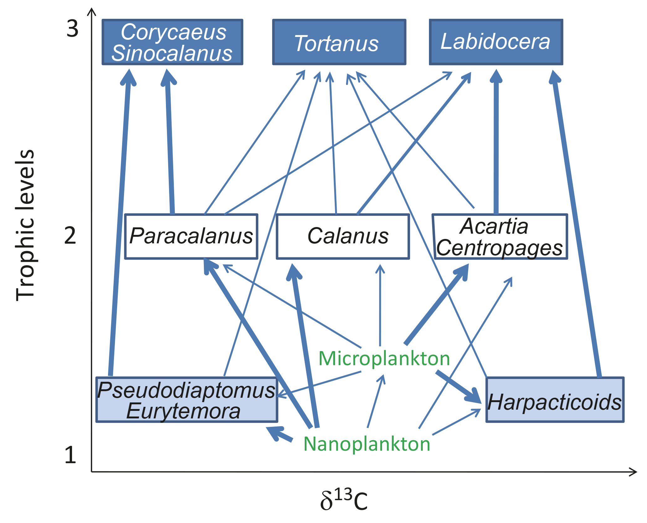
Figure 9A simplified energy flow figure of Gwangyang Bay plankton and copepods. Arrows indicate feeding relationships. Thick arrows indicate feeding preference.

Download

In contrast to both marine calanoids and brackish water calanoids, the cyclopoid species Corycaeus affinis was a carnivorous species preferring to predate on two brackish species – Paracalanus and Pseudodiaptomus (Fig. 8d). This species is widely distributed in all the world's oceans (Turner, 2004) and also frequently dominates in copepod assemblages in spring and autumn in Gwangyang Bay (Table 1). Although the isotopic data for harpacticoid copepods were limited to only one season, we still obtained a clear feeding selectivity pattern based on the Bayesian mixing model (Fig. 7c). Harpacticoids in winter preferred microplankton to nanoplankton if benthic food sources were not considered. Their feeding selectivity contributed to the overall feeding preference of total copepods in this season.