the Creative Commons Attribution 4.0 License.
the Creative Commons Attribution 4.0 License.
 | 15 Mar 2018
Technical note: A simple approach for efficient collection of field reference data for calibrating remote sensing mapping of northern wetlands
Magnus Gålfalk
Martin Karlson
Patrick Crill
Philippe Bousquet
David Bastviken
The calibration and validation of remote sensing land cover products are highly dependent on accurate field reference data, which are costly and practically challenging to collect. We describe an optical method for collection of field reference data that is a fast, cost-efficient, and robust alternative to field surveys and UAV imaging. A lightweight, waterproof, remote-controlled RGB camera (GoPro HERO4 Silver, GoPro Inc.) was used to take wide-angle images from 3.1 to 4.5 m in altitude using an extendable monopod, as well as representative near-ground (< 1 m) images to identify spectral and structural features that correspond to various land covers in present lighting conditions. A semi-automatic classification was made based on six surface types (graminoids, water, shrubs, dry moss, wet moss, and rock). The method enables collection of detailed field reference data, which is critical in many remote sensing applications, such as satellite-based wetland mapping. The method uses common non-expensive equipment, does not require special skills or training, and is facilitated by a step-by-step manual that is included in the Supplement. Over time a global ground cover database can be built that can be used as reference data for studies of non-forested wetlands from satellites such as Sentinel 1 and 2 (10 m pixel size).
- Article
(7194 KB) -
Supplement
(1961 KB) - BibTeX
- EndNote


Accurate and timely land cover data are important for, e.g., economic, political, and environmental assessments, and for societal and landscape planning and management. The capacity for generating land cover data products from remote sensing is developing rapidly. There has been an exponential increase in launches of new satellites with improved sensor capabilities, including shorter revisit time, larger area coverage, and increased spatial resolution (Belward and Skøien, 2015). Similarly, the development of land cover products is increasingly supported by the progress in computing capacities and machine learning approaches.
At the same time it is clear that the knowledge of the Earth's land cover is still poorly constrained. A comparison between multiple state-of-the-art land cover products for West Siberia revealed disturbing uncertainties (Frey and Smith, 2007) as estimated wetland areas ranged from 2 to 26 % of the total area, and the correspondence to in situ observations for wetlands was only 2–56 %. For lakes, all products revealed similar area cover (2–3 %), but the agreement with field observations was as low as 0–5 %. Hence, in spite of the progress in technical capabilities and data analysis progress, there are apparently fundamental factors that still need consideration to obtain accurate land cover information.
The West Siberia example is not unique. Current estimates of the global wetland area range from 8.6 to 26.9 × 10⁶ km2, with great inconsistencies between different data products (Melton et al., 2013). The uncertainty in wetland distribution has multiple consequences, including being a major bottleneck for constraining the assessments of global methane (CH4) emissions (Crill and Thornton, 2017), which was the motivation for this area comparison. Wetlands and lakes are the largest natural CH4 sources (Saunois et al., 2016) and available evidence suggests that these emissions can be highly climate sensitive, particularly at northern latitudes predicted to experience the highest temperature increases and melting permafrost – both contributing to higher CH4 fluxes (Schuur et al., 2009; Yvon-Durocher et al., 2014).
CH4 fluxes from areas with different plant communities in northern wetlands can differ by orders of magnitude (in the following, northern wetlands refer to non-forested boreal, subarctic, and arctic wetlands). Small wet areas dominated by emergent graminoid plants account for by far the highest fluxes m−2, while the more widespread areas covered by, e.g., Sphagnum mosses have much lower CH4 emissions m−2 (e.g., Bäckstrand et al., 2010). The fluxes associated with the heterogeneous and patchy (i.e., mixed) land cover in northern wetlands are well understood on the local plot scale, whereas the large-scale extrapolations are very uncertain. The two main reasons for this uncertainty are that the total wetland extent is unknown and that present map products do not distinguish between different wetland habitats which control fluxes and flux regulation. As a consequence the whole source attribution in the global CH4 budget remains highly uncertain (Kirschke et al., 2013; Saunois et al., 2016).
Improved land cover products relevant to CH4 fluxes and their regulation are therefore needed to resolve this. The detailed characterization of wetland features or habitats requires the use of high-resolution satellite data and sub-pixel classifications that quantify percent, or fractional, land cover. A fundamental bottleneck for the development of fractional land cover products is the quantity and quality of the reference data used for calibration and validation (Foody 2013; Foody et al., 2016). In fact, reference data can often be any data available at higher resolution than the data product, including other satellite imagery and airborne surveys, in addition to field observations. In turn, the field observations can range from rapid landscape assessments to detailed vegetation mapping in inventory plots, where the latter yields high-resolution and high-quality data but is very expensive to generate in terms of time and manpower (Frey and Smith, 2007; Olofsson et al., 2014). Ground-based reference data for fractional land cover mapping can be acquired using traditional methods, such as visual estimation, point frame assessment or digital photography (Chen et al., 2010). These methods can be applied using a transect approach to increase the area coverage in order to match the spatial resolutions of different satellite sensors (Mougin et al., 2014).
The application of digital photography and image analysis software has shown promise for enabling rapid and objective measurements of fractional land cover that can be repeated over time for comparative analysis (Booth et al., 2006a). While several geometrical corrections and photometric setups are used, nadir (downward facing) and hemispherical view photography is most common, and the selected setup depends on the height structure of the vegetation (Chen et al., 2010). Most previous research has however focused on distinguishing between major general categories, such as vegetation and non-vegetation (Laliberte et al., 2007; Zhou and Liu, 2015), and is typically not used to characterize more subtle patterns within major land cover classes. Many applications in the literature have been in rangeland, while there is a lack of wetland classification. Furthermore, images have mainly been close-up images taken from a nadir view perspective (Booth et al., 2006a; Chen et al., 2010; Zhou and Liu, 2015), thereby limiting the spatial extent to well below the pixel size of satellite systems suitable for regional-scale mapping.
From a methano-centric viewpoint, accurate reference data at high enough resolution, being able to separate wetland (and upland) habitats with differing flux levels and regulation, are needed to facilitate progress with available satellite sensors. The resolution should preferably be better than 1 m2 given how the high emitting graminoid areas are scattered on the wettest spots where emergent plants can grow. Given this need, we propose a quick and simple type of field assessment adapted for the 10 × 10 m pixels of the Sentinel 1 and 2 satellites.
Our method uses true color images of the ground, followed by image analysis to distinguish fractional cover of key land cover types relevant to CH4 fluxes from northern wetlands, where we focus on a few classes that differ in their CH4 emissions. We provide a simple manual allowing anyone to take the photos needed in a few minutes per field plot. Land cover classification can then be made using the red–green–blue (RGB) field images (sometimes also converting them to the intensity–hue–saturation (IHS) color space) by software such as, e.g., CAN-EYE (Weiss and Baret, 2010), VegMeasure (Johnson et al., 2003), SamplePoint (Booth et al., 2006b), or eCognition (Trimble commercial software). With this simple approach it would be quick and easy for the community to share such images online and to generate a global reference database that can be used for land cover classification relevant to wetland CH4 fluxes, or other purposes, depending on the land cover classes used. We use our own routines written in Matlab due to the large field of view used in the method, in order to correct for the geometrical perspective when calculating areas (to speed up the development of a global land cover reference database, we can do the classification on request if all necessary parameters and images are available as given in our manual).
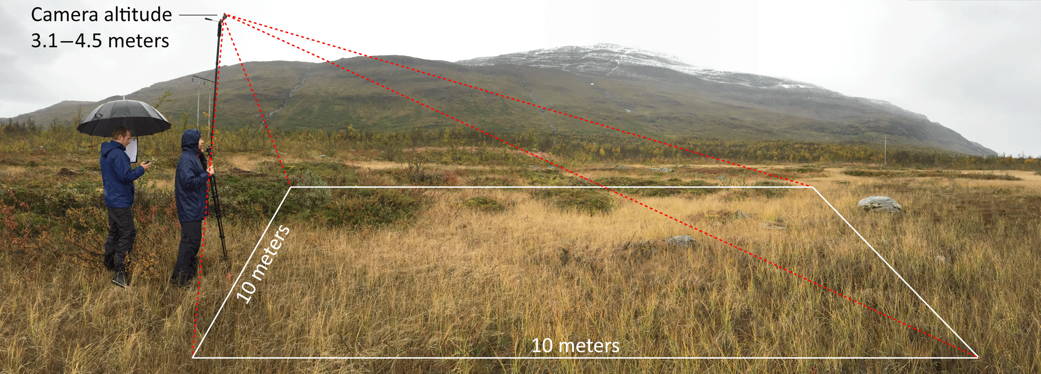
Figure 1A remotely controlled wide-field camera mounted on a long monopod captures the scene in one shot, from above the horizon down to nadir. After using the horizon image position to correct for the camera angle, a 10 × 10 m area close to the camera is used for classification.
Figure 2Correction of lens distortion. (a) Raw wide-field camera image. (b) After correction.
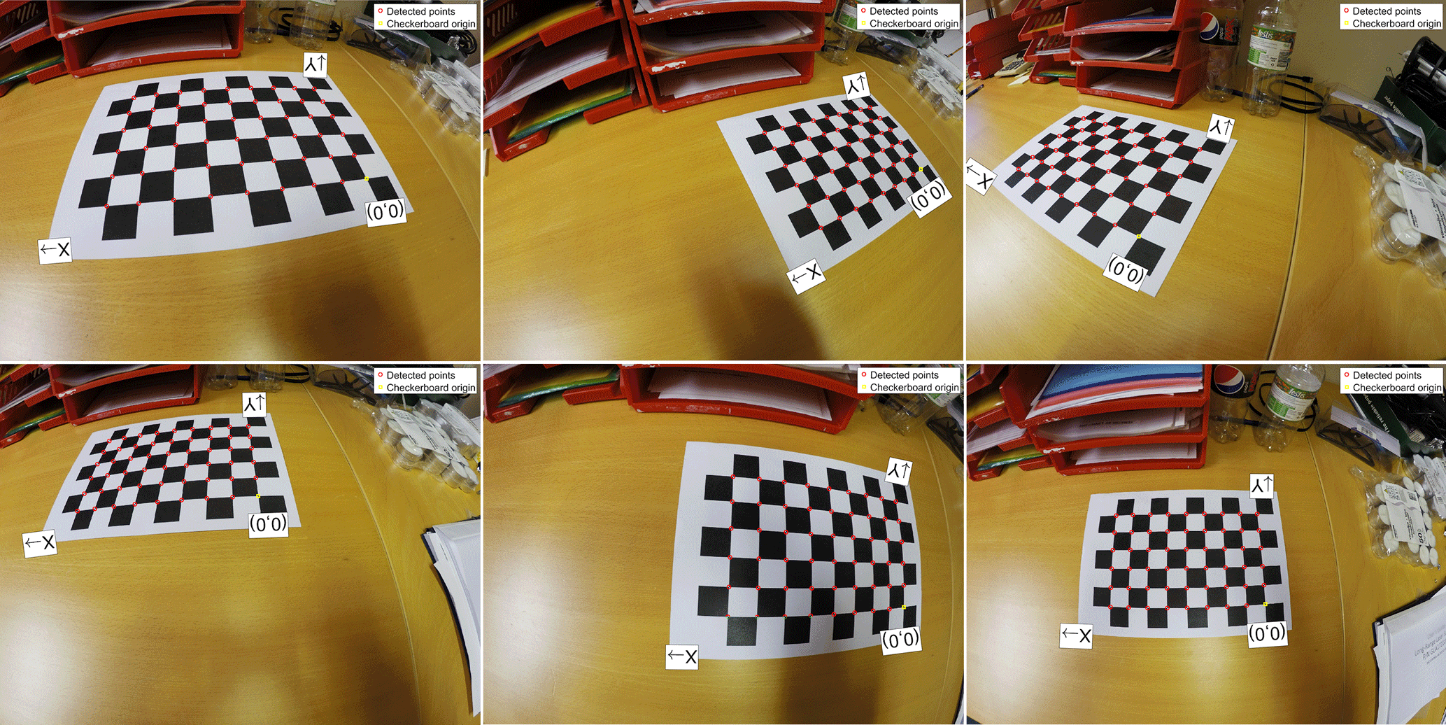
Figure 3Modeling of lens distortion. Checkboard pattern used for calibrations. Red circles are used to mark automatically detected square corners, while the yellow square marks the origin of the coordinate system. Images of the pattern are taken from 10 to 20 different camera angles.
The camera setup is illustrated in Fig. 1, with lines showing the spatial extent of a field plot. Our equipment included a lightweight RGB camera (GoPro 4 Hero Silver; other types of cameras with remote control and a suitable wide field of view would also work) mounted on an extendable monopod that allows imaging from a height of 3.1–4.5 m. The camera had a resolution of 4000 × 3000 pixels with a wide field of view (FOV) of 122.6 × 94.4∘ and was remotely controlled over Bluetooth using a cellphone application that allows a live preview, making it possible to always include the horizon close to the upper edge in each image (needed for image processing later – see below). The camera had a waterproof casing and could therefore be used in rainy conditions, making the method robust to variable weather conditions. Measurements were made for about 200 field plots in northern Sweden in the period 6–8 September 2016.
For each field plot, the following were recorded.
-
One image taken at > 3.1 m height (see illustration in Fig. 1) which includes the horizon coordinate close to the top of the image
-
Three to four close-up images of the most common surface cover types in the plot (e.g., typical vegetation) and a very short note for each image indicating what is shown, e.g., whether a close-up image shows dry or wet moss (two of our classes), as there can be different colors within a class.
-
GPS position of the camera location (reference point)
-
Notes of the image direction relative to the reference point
A long modified monopod with a GoPro camera mounted at the end was used for the imaging. The geographic coordinate of the camera position was registered using a handheld Garmin Oregon 550 GPS with a horizontal accuracy of approximately 3 m. The positional accuracy of the images can be improved by using a differential GPS and by registering the cardinal direction of the FOV. The camera battery lasted for a few hours after a full charge, but was charged at intervals when not used, e.g., when moving between different field sites, making it possible to do all the imaging using only one camera.
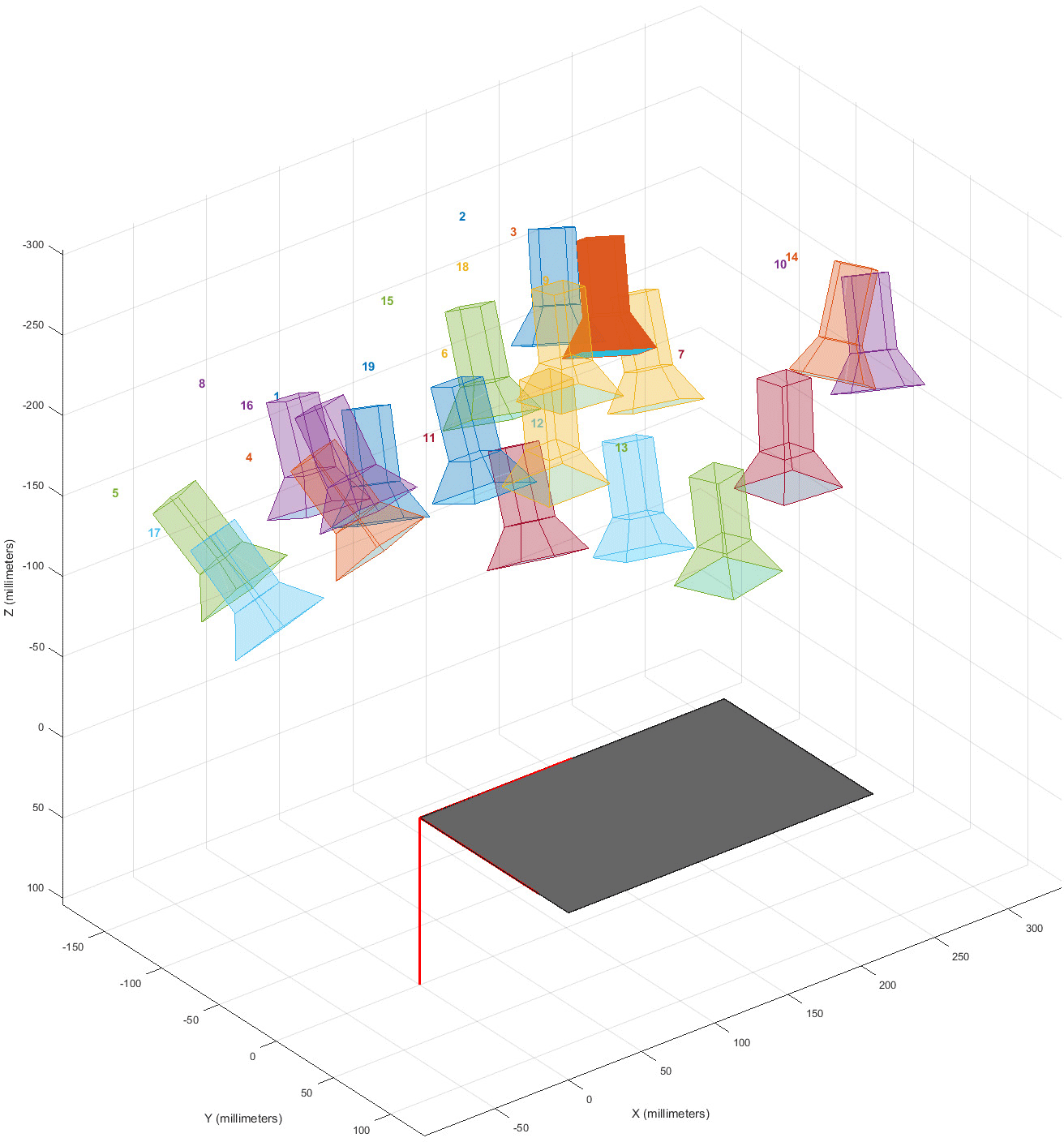
Figure 4Illustration using Matlab's Camera calibration application of the camera positions used when taking the calibration images.
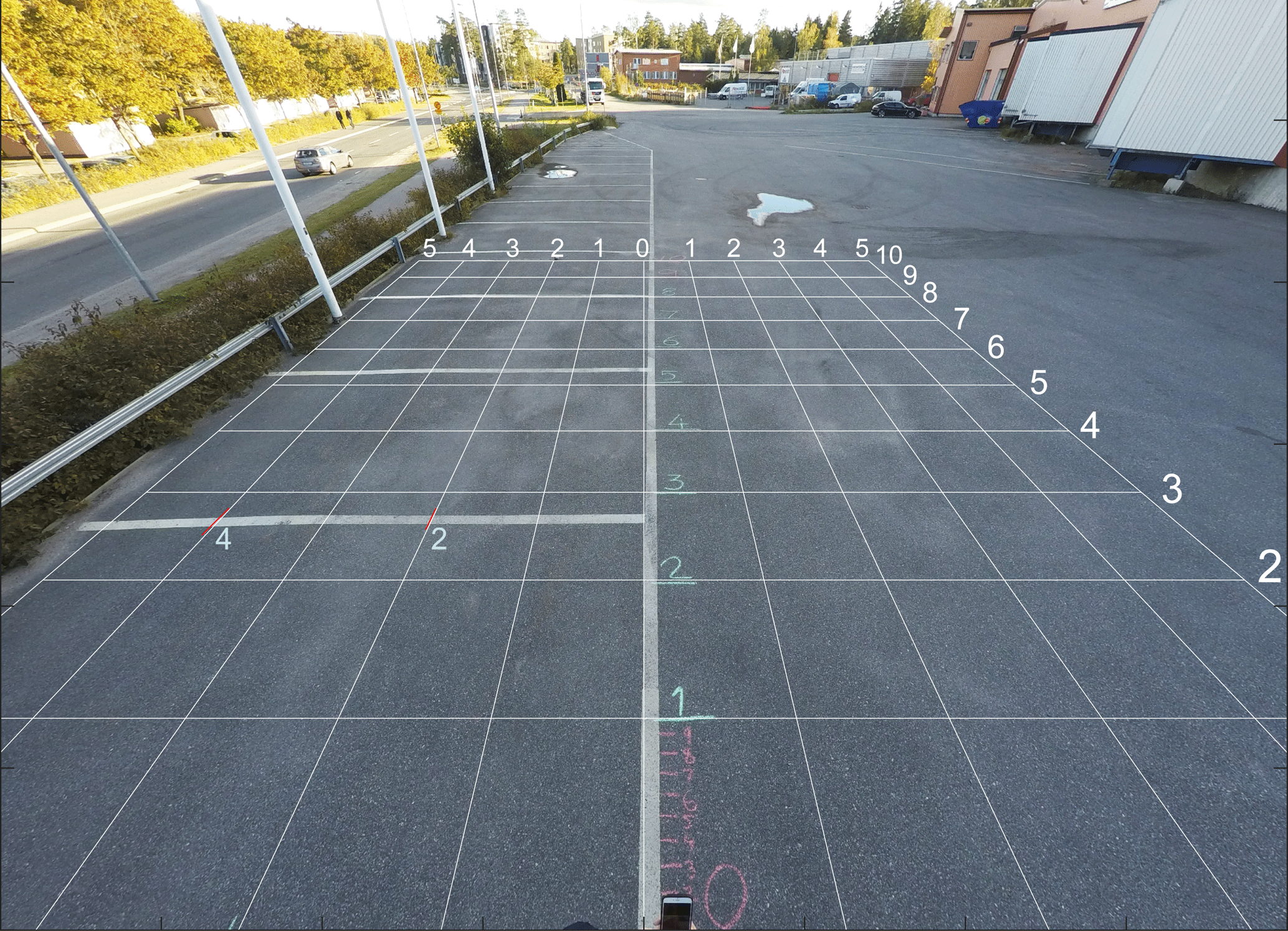
Figure 5Calibration of projected geometry using an image corrected for lens distortion. Model geometry is shown as white numbers and a white grid, while green and red numbers are written on the ground using chalk (red lines at 2 and 4 m left of the center line were strengthened for clarity). The camera height in this calibration measurement is 3.1 m.
As the camera had a very wide FOV, the raw images do have a strong lens distortion (Fig. 2). This can be corrected for many camera models (e.g., the GoPro series) using ready-made models in Adobe Lightroom or Photoshop, or by modeling the distortion for any camera using the camera calibrator application in Matlab's computer vision system toolbox as described below. A checkboard pattern is needed for the modeling (Fig. 3), which should consist of black and white squares with an even number of squares in one direction and an odd number of squares in the other direction, preferably with a white border around the pattern. The next step is to take images of this pattern from 10 to 20 unique camera positions, providing many perspectives of the pattern with different angles for the distortion modeling (Fig. 3). In order to make accurate models, it is important both to have sharp images with no motion blur (e.g., due to movement or poor lighting) and to include several images where the pattern is close to the edges of the image, as this is where the distortion is greatest. An alternative but equivalent method, preferably used for small calibration patterns printed on a standard sheet of paper (e.g., letter or A4), is to mount the camera and instead move the paper to 10–20 unique positions with different angles to the camera. A quick way to do this with only one person present is by recording a video while moving the paper slowly and then selecting calibration images from the video afterwards. The illustration of camera positions used (Fig. 4) can also be displayed in the application as a mounted camera with different positions of the calibration pattern. The next step is to enter the size of a checkerboard square (mm, cm, or in) which is followed by an automatic identification of the corners of squares in the pattern (Fig. 3). Images with bad corner detection can now be removed (optional) to improve the modeling. As a last step, camera parameters can now be calculated with the press of a button and be saved as a variable in Matlab (cameraParams). This whole procedure only has to be done once for each camera and FOV setting used, meaning once for a data collection campaign or a project if the same camera model and FOV are used. Applying the correction to images is done using a single command in Matlab: img_corr = undistortImage(img, cameraParams). Here img and img_corr are variables for the uncorrected and corrected versions, respectively.
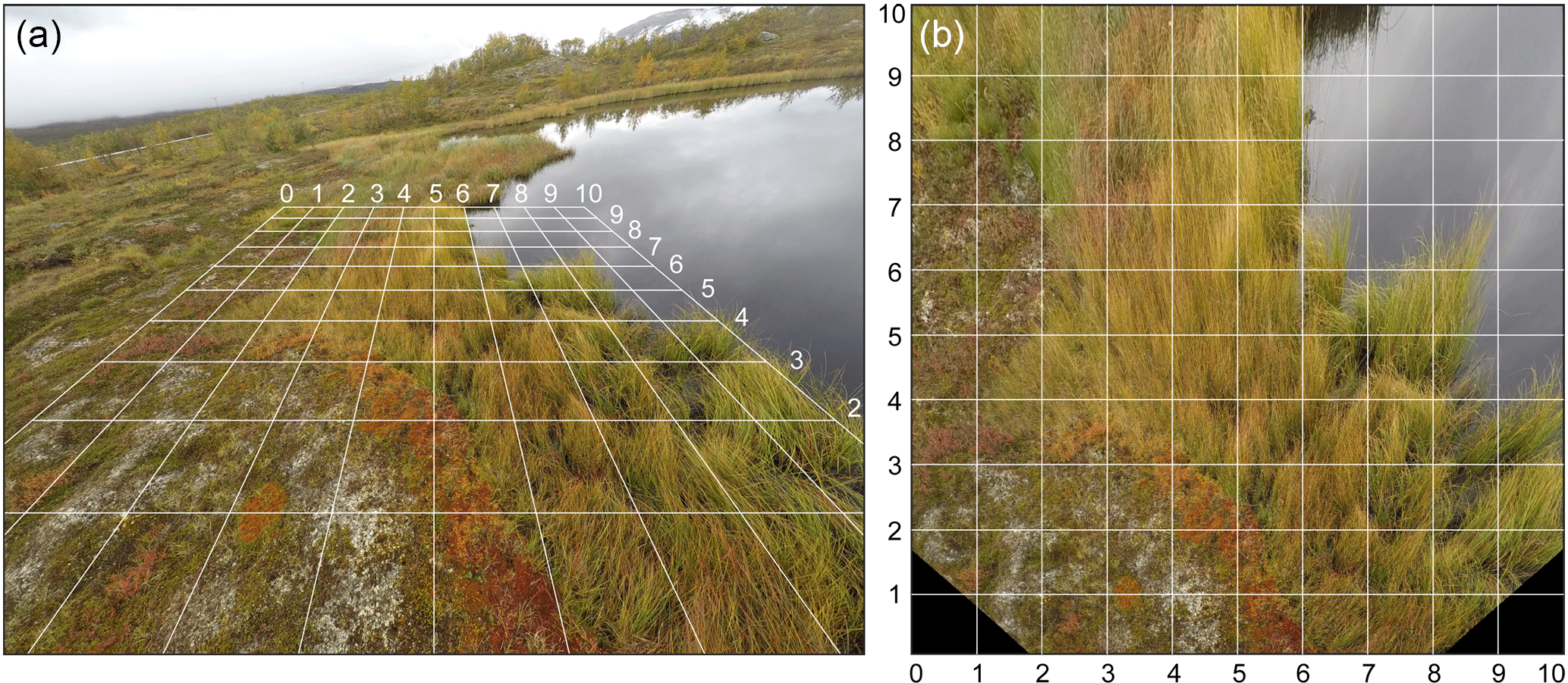
Figure 6One of our field plots. (a) Image corrected for lens distortion, with a projected 10 × 10 m grid overlaid. (b) Image after recalculation to overhead projection (10 × 10 m).
Using a distortion-corrected calibration image, we then developed a model of the ground geometry by projecting and fitting a 10 × 10 m grid on a parking lot with measured distances marked using chalk (Fig. 5). Such calibration of projected ground geometry only needs to be done when changing the camera model or field of view setting, and is valid for any camera height as long as the heights used in the field and in the calibration imaging are known. It is done quickly by drawing short lines every meter for distances up to 10 m, and some selected perpendicular lines at strategic positions to obtain the perspective. At least one, and preferably two, perpendicular distances should be marked at a minimum of two different distances along the central line (in Fig. 5 at 2 and 4 m left of the central line at distances along the central line of 0 and 2.8 m). The geometric model uses the camera FOV, camera height, and vertical coordinate of the horizon (to obtain the camera angle). We find excellent agreement between the modeled and measured grids (fits are within a few centimeters) for both camera heights of 3.1 and 4.5 m.
The vertical angle α from nadir to a certain point on the grid with ground distance Y along the center line is given by , where h is the camera height. For distance points in our calibration image (Fig. 5), using 0.2 m steps in the range 0–1 m and 1 m steps from 1 to 10 m, we calculate the nadir angles α(Y) and measure the corresponding vertical image coordinates ycalib(Y).
In principle, for any distortion corrected image there is a simple relationship , where yimg is the image vertical pixel coordinate for a certain distance Y, PFOV the pixel field of view (deg pixel−1), and α0 the nadir angle of the bottom image edge. In practice, however, correction for lens distortion is not perfect, so we have fitted a polynomial in the calibration image to obtain ycalib(α) from the known α and measured ycalib. Using this function we can then obtain the yimg coordinate in any subsequent field image using
where and are the vertical image coordinates of the horizon in the field and calibration image, respectively. As the PFOV varies by a small amount across the image due to small deviations in the lens distortion correction, we have used PFOVhor, which is the pixel field of view at the horizon coordinate. In short, the shift in horizon position between the field and calibration images is used to compensate for the camera having different tilts in different images. In order to obtain correct ground geometry it is therefore important to always include the horizon in all images.
The horizontal ground scale dx (pixels m−1) varies linearly with yimg, making it possible to calculate the horizontal image coordinate ximg using
where dx0 is the horizontal ground scale at the bottom edge of the calibration image, xc the center line coordinate (half the horizontal image size), X the horizontal ground distance, and hcalib and himg the camera heights in the calibration and field image, respectively.
Thus, using Eqs. (1) and (2) we can calculate the image coordinates (ximg, yimg) in a field image from any ground coordinates (X, Y). A model grid is shown in Fig. 5 together with the calibration image, illustrating their agreement.
For each field image, after correction for image distortion, our Matlab script asks for the y-coordinate of the horizon (which is selected using a mouse). This is used to calculate the camera tilt and to over-plot a distance grid projected on the ground (Fig. 6a). Using Eqs. (1) and (2) we then recalculate the image to an overhead projection of the nearest 10 × 10 m area (Fig. 6b). This is done using interpolation, where a (ximg, yimg) coordinate is obtained from each (X, Y) coordinate, and the brightness in each color channel (R, G, B) calculated using sub-pixel interpolation. The resulting image is reminiscent of an overhead image, with equal scales in both axes. There is however a small difference, as the geometry (due to the line of sight) does not provide information about the ground behind high vegetation in the same way as an image taken from overhead. In cases with high vegetation (which is some of our 200 field plots), mostly high grass, we used a higher camera altitude to decrease obscured areas. Another possibility is to direct the camera towards nadir (see the manual in Supplement S1) to image areas −5 to +5 m from the center of a plot, further decreasing the viewing angles from nadir. We did not have any problems with shrub or brushwood as it was only a couple of dm high, and birch trees did not grow on the mires. We also recommend using a camera height of about 6 m to decrease obscuration and to increase the mapped area.
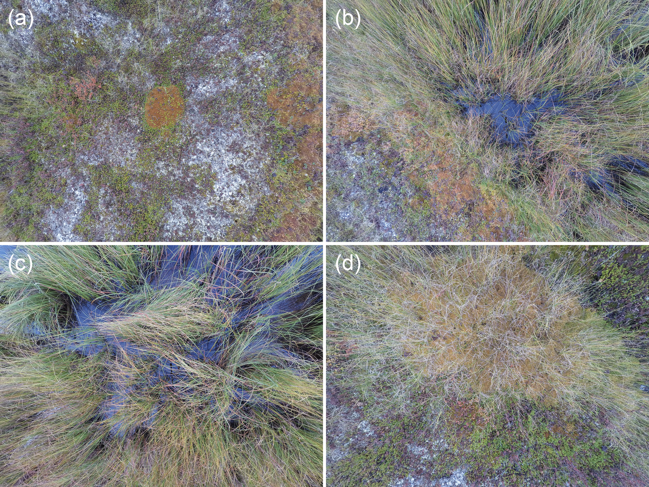
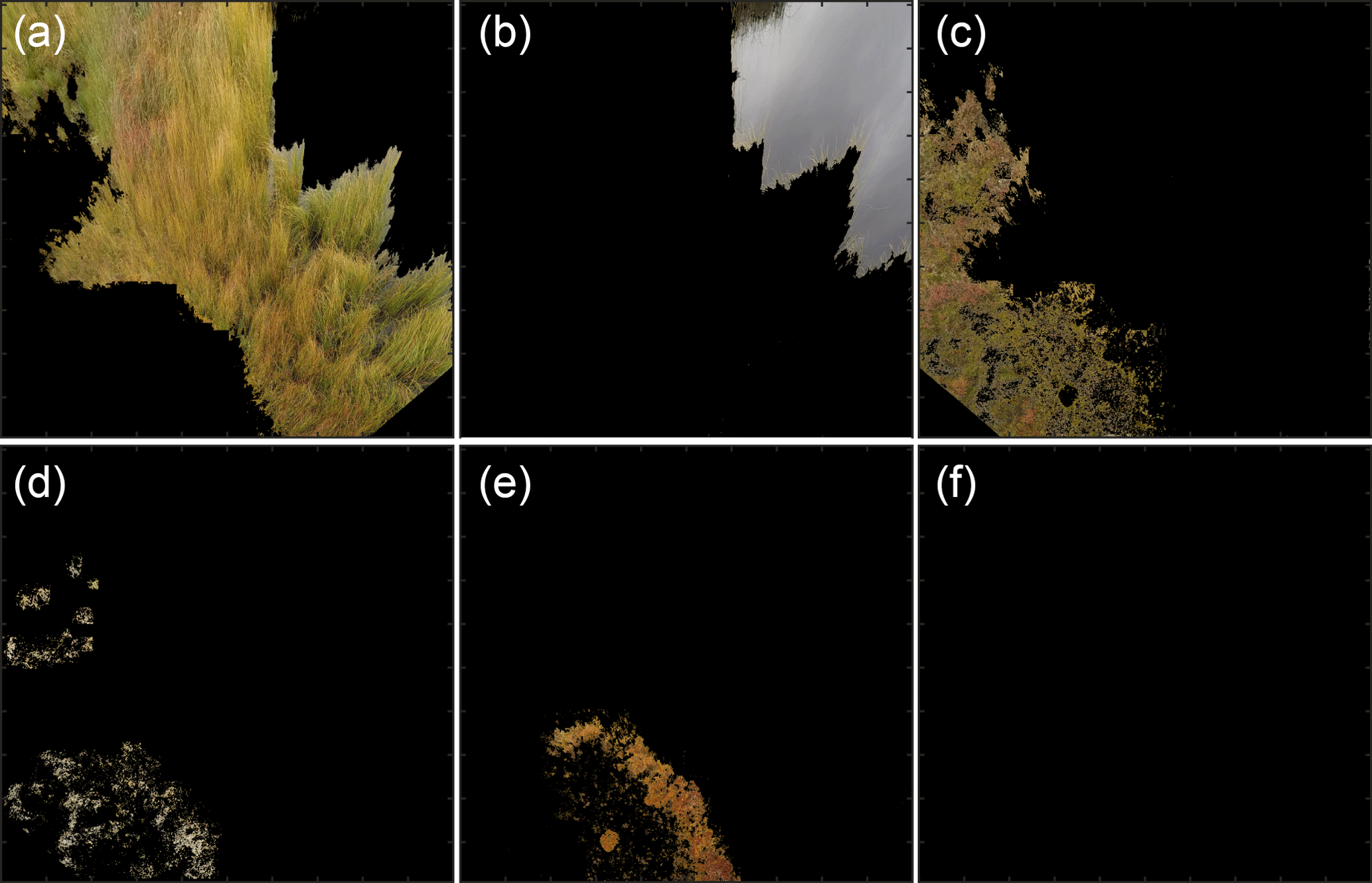
Figure 8Classification of a field plot image (Fig. 6b) into the six main surface components. All panels have an area of 10 × 10 m. (a) Graminoids, (b) water, (c) shrubs, (d) dry moss, (e) wet moss, (f) rock.
After a field plot has been geometrically rectified, so that the spatial resolution is the same over the surface area used for classification, the script distinguishes land cover types by color, brightness and spatial variability. Aided by the close-up images of typical surface types also taken at each field plot (Fig. 7) and short field notes about the vegetation, providing further verification, a script is applied to each overhead-projected calibration field (Fig. 6b) that classifies the field plot into land cover types. This is a semi-automatic method that can account for illumination differences between images. In addition, it facilitates identification, as there can for instance be different vegetation with similar color, and rock surfaces that have a similar appearance to water or vegetation. After an initial automatic classification, the script has an interface that allows manual reclassification of areas between classes. The close-up images have high detail richness, allowing identification, and color and texture assignment of the different land cover classes during similar light and weather conditions as when the whole-plot image is taken. This makes results robust regarding different users collecting data, with respect to light conditions, times of day, etc. The sensitivity is instead affected by the person defining the classes, just as with normal visual inspection.
For calculations of surface color we filter the overhead projected field images using a running 3 × 3 pixel mean filter, providing more reliable statistics. Spatial variation in brightness, used as a measurement of surface roughness, is calculated using a running 3 × 3 pixel standard deviation filter. Denoting the brightness in each (red, green, and blue) color channel R, G and B, respectively, we could for instance find areas with green grass using the green filter index , where a value above 1 indicates green vegetation. In the same way, areas with water (if the close-up images show blue water due to clear sky) can be found using a blue filter index . If the close-up images show dark or gray water (cloudy weather), it can be distinguished from rock and white vegetation using either a total brightness index or an index that is sensitive to surface roughness, involving σ(R), σ(G), or σ(B), where σ denotes the 3 × 3 pixel standard deviation centered on each pixel, for a certain color channel.
In this study we used six different land cover types of relevance to CH4 regulation: graminoids, water, shrubs, dry moss, wet moss, and rock. Examples of classified images are shown in Fig. 8. Additional field plots and classification examples can be found in Supplement S2. Compared to the corrections for lens distortion and geometrical projection, the classification part often takes the longest time, as it is semi-automatic and requires trial and error testing of which indices and class limits to use for each image as vegetation and lighting conditions might vary. After a number of images with similar vegetation and conditions have been classified, the process goes much faster as the indices and limits will be roughly the same. One may also need to reclassify parts manually by moving a square region from one class to another based on visual inspection. The main advantage with this method of obtaining reference data is however that it is very fast in the field and works in all weather conditions. In a test study, we were able to make classifications of about 200 field plots in northern Sweden in a 3-day test campaign despite rainy and windy conditions. For each field plot, surface area (m2) and coverage (%) were calculated for each class. The geometrical correction models (lens distortion and ground projection) were made in about an hour, while the classifications for all plots took a few days.
This study describes a quick method to document ground surface cover and process the data to make them suitable as reference data for remote sensing. The method requires a minimum of equipment that is frequently used by researchers and persons with general interest in outdoor activities, and image recording can be made easily and in a few minutes per plot without requirements of specific skills or training. In addition to covering large areas in a short time, it is a robust method that works in any weather using a waterproof camera. This provides an alternative to, e.g., using small unmanned aerial vehicles (UAVs) which are efficient at covering large areas but have the drawbacks of being sensitive to both wind and rain and typically having flight times of about 20 min (considerably lower if many takeoffs and landings are needed when moving between plots). The presented photographic approach is also possible using a mobile phone camera, although such cameras usually have a very small field of view compared to many adventure cameras (such as the GoPro, which is also cheaper than a cellphone). We recommend using a higher camera altitude; a height of 6 m would make mobile phone imaging of 10 × 10 m possible (using a remote Bluetooth controller) and 20 × 20 m mapping using a camera with a large field of view such as the GoPro. Hence, if the method becomes widespread and a fraction of those who visit northern wetlands (or other environments without dense tall vegetation where the method is suitable) contribute images and related information, there is a potential for rapid development of a global database of images and processed results with detailed land cover for individual satellite pixels. In turn, this could become a valuable resource supplying reference data for remote sensing. To facilitate this development, Supplement S1 includes a complete manual and the authors will assist with early stage image processing and initiate database development.
The data used in this article are a small subset of our approximately 200 field plots, only used as examples to illustrate the steps of the method. More examples are given in the Supplement. The full dataset of field reference data will be published in a future database.
The supplement related to this article is available online at: https://doi.org/10.5194/bg-15-1549-2018-supplement.
The authors declare that they have no conflict of interest.
This study was funded by a grant from the Swedish Research Council VR to
David Bastviken (ref. no. VR 2012-48). We would also like to acknowledge the
collaboration with the IZOMET project (ref. no. VR 2014-6584) and IZOMET
partner Marielle Saunois (Laboratoire des Sciences du Climat et de
l'Environnement (LSCE), Gif-sur-Yvette, France).
Edited by: Paul Stoy
Reviewed by: two
anonymous referees
Belward, A. S. and Skøien, J. O.: Who launched what, when and why; trends in global land-cover observation capacity from civilian earth observation satellites, ISPRS J. Photogramm., 103, 115–128, 2015.
Booth, D. T., Cox, S. E., Meikle, T. W., and Fitzgerald, C.: The accuracy of ground cover measurements, Rangeland Ecol. Manag., 59, 179–188, 2006a.
Booth, D. T., Cox, S. E., and Berryman, R. D.: Point sampling digital imagery with “SamplePoint”, Environ. Monit. Assess., 123, 97–108, 2006b.
Bäckstrand, K., Crill, P. M., Jackowicz-Korczyñski, M., Mastepanov, M., Christensen, T. R., and Bastviken, D.: Annual carbon gas budget for a subarctic peatland, Northern Sweden, Biogeosciences, 7, 95–108, https://doi.org/10.5194/bg-7-95-2010, 2010.
Chen, Z., Chen, W., Leblanc, S. G., and Henry, G. H. R.: Digital Photograph Analysis for Measuring Percent Plant Cover in the Arctic, Arctic, 63, 315–326, 2010.
Crill, P. M. and Thornton, B. F.: Whither methane in the IPCC process?, Nat. Clim. Change, 7, 678–680, 2017.
Frey, K. E. and Smith, L. C.: How well do we know northern land cover? Comparison of four global vegetation and wetland products with a new ground-truth database for West Siberia, Global Biogeochem. Cy., 21, GB1016, https://doi.org/10.1029/2006GB002706, 2007.
Foody, G. M.: Ground reference data error and the mis-estimation of the area of land cover change as a function of its abundance, Remote Sens. Lett., 4, 783–792, 2013.
Foody, G. M., Pal, M., Rocchini, D., Garzon-Lopez, C. X., and Bastin, L.: The Sensitivity of Mapping Methods to Reference Data Quality: Training Supervised Image Classifications with Imperfect Reference Data, ISPRS Int. J. Geo.-Inf., 5, 199, https://doi.org/10.3390/ijgi5110199, 2016.
Johnson, D. E, Vulfson, M., Louhaichi, M., and Harris, N. R.: VegMeasure version 1.6 user's manual, Oregon State University, Department of Rangeland Resources, Corvallis, OR, USA, 2003.
Kirschke, S., Bousquet, P., Ciais, P., et al.: Three decades of global methane sources and sinks, Nat. Geosci., 6, 813–823, 2013.
Laliberte, A. S., Rango, A., Herrick, J. E., Fredrickson, E. L., and Burkett, L.: An object-based image analysis approach for determining fractional cover of senescent and green vegetation with digital plot photography, J. Arid Environ,, 69, 1–14, 2007.
Melton, J. R., Wania, R., Hodson, E. L., Poulter, B., Ringeval, B., Spahni, R., Bohn, T., Avis, C. A., Beerling, D. J., Chen, G., Eliseev, A. V., Denisov, S. N., Hopcroft, P. O., Lettenmaier, D. P., Riley, W. J., Singarayer, J. S., Subin, Z. M., Tian, H., Zürcher, S., Brovkin, V., van Bodegom, P. M., Kleinen, T., Yu, Z. C., and Kaplan, J. O.: Present state of global wetland extent and wetland methane modelling: conclusions from a model inter-comparison project (WETCHIMP), Biogeosciences, 10, 753–788, https://doi.org/10.5194/bg-10-753-2013, 2013.
Mougin, E., Demarez, V., Diawara, M., Hiernaux, P., Soumaguel, N., and Berg, A.: Estimation of LAI, fAPAR and fCover of Sahel rangelands, Agr. Forest Meteorol., 198–199, 155–167, 2014.
Olofsson, P., Foody, G. M., Herold, M., Stehman, S. V., Woodcock, C. E., and Wulder, M. A.: Good practices for estimating area and assessing accuracy of land change, Remote Sens. Environ., 148, 42–57, 2014.
Saunois, M., Bousquet, P., Poulter, B., Peregon, A., Ciais, P., Canadell, J. G., Dlugokencky, E. J., Etiope, G., Bastviken, D., Houweling, S., Janssens-Maenhout, G., Tubiello, F. N., Castaldi, S., Jackson, R. B., Alexe, M., Arora, V. K., Beerling, D. J., Bergamaschi, P., Blake, D. R., Brailsford, G., Brovkin, V., Bruhwiler, L., Crevoisier, C., Crill, P., Covey, K., Curry, C., Frankenberg, C., Gedney, N., Höglund-Isaksson, L., Ishizawa, M., Ito, A., Joos, F., Kim, H.-S., Kleinen, T., Krummel, P., Lamarque, J.-F., Langenfelds, R., Locatelli, R., Machida, T., Maksyutov, S., McDonald, K. C., Marshall, J., Melton, J. R., Morino, I., Naik, V., O'Doherty, S., Parmentier, F.-J. W., Patra, P. K., Peng, C., Peng, S., Peters, G. P., Pison, I., Prigent, C., Prinn, R., Ramonet, M., Riley, W. J., Saito, M., Santini, M., Schroeder, R., Simpson, I. J., Spahni, R., Steele, P., Takizawa, A., Thornton, B. F., Tian, H., Tohjima, Y., Viovy, N., Voulgarakis, A., van Weele, M., van der Werf, G. R., Weiss, R., Wiedinmyer, C., Wilton, D. J., Wiltshire, A., Worthy, D., Wunch, D., Xu, X., Yoshida, Y., Zhang, B., Zhang, Z., and Zhu, Q.: The global methane budget 2000–2012, Earth Syst. Sci. Data, 8, 697–751, https://doi.org/10.5194/essd-8-697-2016, 2016.
Schuur, E. A. G., Vogel, J. G., Crummer, K. G., Lee, H., Sickman, J. O., and Osterkamp, T. E.: The effect of permafrost thaw on old carbon release and net carbon exchange from tundra, Nature, 459, 556–559, 2009.
Weiss, M. and Baret, F.: CAN-EYE V6.4.6 User Manual, EMMAH laboratory (Mediterranean environment and agro-hydro system modelisation), National Institute of Agricultural Research (INRA), 2010.
Yvon-Durocher, G., Allen, A. P., Bastviken, D., Conrad, R., Gudasz, C., St-Pierre, A., Thanh-Duc, N., and del Giorgio, P. A.: Methane fluxes show consistent temperature dependence across microbial to ecosystem scales, Nature, 507, 488–491, 2014.
Zhou, G. and Liu, S.: Estimating ground fractional vegetation cover using the double-exposure method, Int. J. Remote Sens., 36, 6085–6100, 2015.